Bias-Corrected Peaks-Over-Threshold Estimation of the CVaR

Abstract

The conditional value-at-risk (CVaR) is a useful risk measure in fields such as machine learning, finance, insurance, energy, etc. When measuring very extreme risk, the commonly used CVaR estimation method of sample averaging does not work well due to limited data above the value-at-risk (VaR), the quantile corresponding to the CVaR level. To mitigate this problem, the CVaR can be estimated by extrapolating above a lower threshold than the VaR using a generalized Pareto distribution (GPD), which is often referred to as the peaks-over-threshold (POT) approach. This method often requires a very high threshold to fit well, leading to high variance in estimation, and can induce significant bias if the threshold is chosen too low. In this paper, we derive a new expression for the GPD approximation error of the CVaR, a bias term induced by the choice of threshold, as well as a bias correction method for the estimated GPD parameters. This leads to the derivation of a new estimator for the CVaR that we prove to be asymptotically unbiased. In a practical setting, we show through experiments that our estimator provides a significant performance improvement compared with competing CVaR estimators in finite samples. As a consequence of our bias correction method, it is also shown that a much lower threshold can be selected without introducing significant bias. This allows a larger portion of data to be be used in CVaR estimation compared with the typical POT approach, leading to more stable estimates. As secondary results, a new estimator for a second-order parameter of heavy-tailed distributions is derived, as well as a confidence interval for the CVaR which enables quantifying the level of variability in our estimator.

1 Introduction

Traditional machine learning algorithms typically consider the expected value of a random variable as the target to optimize. In a risk-averse setting, the objective function needs to be adapted to consider the full distribution and account for severe outcomes. Recently, risk-averse machine learning has become an important area of study, especially in the context of multi-armed bandits and reinforcement learning, for example, for example, Chow and Ghavamzadeh, (2014); Tamar et al., (2015); Torossian et al., (2019); Hiraoka et al., (2019) and Keramati et al., (2020) address learning with a risk-averse agent. Most often, the risk measure of interest is the conditional value-at-risk (CVaR). Given a continuous random variable $X$ representing losses (i.e., where larger values are less desirable), the CVaR at a confidence level $\alpha\in(0,1)$ measures the expected value of $X$ given that $X$ exceeds the quantile of level $\alpha.$ This quantile is referred to as the value-at-risk (VaR). Compared to the VaR, the CVaR captures more information about the weight of a distribution’s tail, making it a more useful object of study in risk-averse decision making. In practice, the CVaR is usually estimated by averaging observations above the estimated VaR, which we call the sample average estimator of the CVaR. When $\alpha$ is close to $1$, these observations can be very scarce in small samples leading to volatile estimates of the CVaR. This work is motivated by a lack of reliable estimators and performance guarantees for the CVaR at these extreme levels. In this paper, we consider estimating the CVaR of heavy-tailed random variables, which are ubiquitous in application domains such as finance, insurance, energy, and epidemiology, e.g., Manz and Mansmann, (2020). In this setting, extreme events correspond to very large observations (and hence severe losses), which is in contrast to the light- or short-tailed cases where similar low probability events are closer to the mean. Extreme value theory provides the tools to construct a new CVaR estimator that is appropriate for this setting. By selecting a threshold lower than the VaR, it is possible to approximate the tail distribution of a random variable by using a generalized Pareto distribution (GPD) and extrapolating beyond available observations. The estimation of quantities using this approximation is commonly referred to as the peaks-over-threshold (POT) approach. An estimator for the CVaR using the POT approach is given in, for example, McNeil et al., (2005, Section 7.2.3), where the CVaR is referred to as the expected shortfall. However, this estimator suffers from one of the main drawbacks of the POT approach, which is the difficult bias-variance tradeoff in selecting the threshold. Unless the threshold is chosen very high, the estimator will encounter two sources of potentially significant bias:

1. The deviation between the GPD and the true tail distribution;

2. The bias associated with parameter estimation using the approximate GPD tail data.

Perhaps even more significantly, the CVaR estimator of McNeil et al., (2005) comes with no performance guarantees unless one assumes exactness of the GPD approximation and of the empirical distribution function, so it has not been previously possible to determine the precise conditions where using the POT approach for CVaR estimation is actually superior to the more common sample average estimator. The goal of this paper is to make a significant refinement to the existing CVaR estimator based on the POT approach and correct the sources of bias induced by the GPD approximation, resulting in a more accurate estimator that is less sensitive to the choice of threshold, as well as to derive performance guarantees in the form of confidence intervals.

Related work. Threshold selection methods for the GPD approximation have been well-studied, for an overview of such methods, see Scarrott and MacDonald, (2012). A recent and empirically successful threshold selection method is given in Bader et al., (2018), and has been applied in Zhao et al., (2018) to estimate the VaR at extreme levels using the POT approach. Estimation of the CVaR using the POT approach has been applied in, for example, Gilli and Këllezi, (2006); Marinelli et al., (2007); Bah et al., (2016); Gkillas and Katsiampa, (2018) and Szubzda and Chlebus, (2019). To the best of our knowledge, results in the literature using the POT approach for risk estimation are presented mostly in the form of empirical studies. On the theoretical side, asymptotic analysis of the deviation in (i) with respect to the underlying distribution can be found in Raoult and Worms, (2003), and Beirlant et al., (2003) considers the deviation with respect to quantile approximations based on the GPD tail model. Bias correction methods for (ii) have been developed in, for example, Peng, (1998); Gomesa and Martins, (2002); Beirlant et al., (2009) and Haouas et al., (2018). These works target the estimation of $\xi$, the shape parameter of the GPD. A central idea is to employ the theory of second-order regular variation to establish asymptotically unbiased extensions of the well-known Hill estimator of $\xi$. However, maximum likelihood estimation is considered the most efficient parameter estimation method for the GPD (see de Zea Bermudez and Kotz, (2010, Section 7)) and targets both $\xi$ and the $\sigma$ (the scale parameter of the GPD). This paper is, to the best of our knowledge, the first to address (ii) for maximum likelihood estimation in view of application. In terms of performance guarantees, concentration bounds for the CVaR estimated by sample averaging exist in the literature, which measure the probability of deviation between the CVaR estimate and its true value for a given sample size. While a major benefit with concentration bounds is that they provide a guaranteed bound in finite samples, it is usually not possible or impractical to apply them to heavy-tailed random variables. For example, Brown, (2007); Thomas and Learned-Miller, (2019) derive concentration bounds which apply to bounded random variables. The concentration bounds of Kolla et al., (2018, 2019); Bhat and L.A., (2019) can be used for heavy-tailed random variables but require distribution-dependent constants, making them impractical. Kagrecha et al., (2019) give concentration bounds which can apply to heavy-tailed random variables without exact distributional knowledge, but their bound is based on a truncated version of the sample average CVaR estimator and requires selecting parameters based on moment bounds of the underlying random variable. An alternative to concentration bounds is to use estimated asymptotic confidence intervals, which typically become good approximations in large sample sizes. Asymptotic confidence intervals for the CVaR using sample average estimation can be found in Trindade et al., (2007); Brazauskas et al., (2008) and Sun and Hong, (2010). These confidence intervals only apply to random variables with bounded variance, which excludes many heavy-tailed random variables. Therefore, it is often not possible to establish measures of uncertainty for CVaR estimates using either the sample average method or the original POT method in the heavy-tailed domain, and this paper aims to address this problem with a rigorous formulation of a new CVaR estimator using the POT approach.

Major contributions. First, we derive the GPD approximation error, a deterministic quantity measuring the deviation between the GPD approximation of the CVaR and its true value. We then derive bias-corrected maximum likelihood estimators for the GPD parameters, $\xi$ and $\sigma$, using the POT approach, which in turn requires the derivation of a new estimator for a second-order parameter that may be of independent interest. Using our bias correction methods, a new estimator for the CVaR based on the POT approach is derived which we prove is asymptotically unbiased. Using our convergence result for the bias-corrected CVaR estimator, we derive a confidence interval for the CVaR which has asymptotically correct coverage probability.

The remainder of this paper is organized as follows. In section 2, the VaR and CVaR are formally defined, and the sample average estimator of the CVaR is given. Needed background from extreme value theory and second-order regular variation is discussed and we formalize the notion of heavy-tailed random variables. The CVaR approximation using the POT approach is given. Section 3 derives the GPD approximation error for the CVaR and its asymptotic behaviour. In section 4, bias-corrected maximum likelihood estimators for the GPD parameters using the POT approach are derived. These estimators are then used in a CVaR estimator with partial bias correction and its asymptotic normality is derived. Section 5 establishes an estimator for the GPD approximation error, and our results are consolidated to give the unbiased POT estimator for the CVaR. Its asymptotic normality is derived and a confidence interval is given. Section 6 gives details on second-order parameter estimation, which plays an important role in bias correction. In section 7, simulations are shown to provide empirical evidence of the finite sample performance of our estimator on data. Section 8 concludes, with directions for future work. All proofs are given in appendix A.

2 Preliminaries

Let $X$ denote a random variable and $F$ its corresponding cumulative distribution function (cdf). In this paper, we adopt the convention that $X$ represents a loss, so larger values of $X$ are less desirable.

Definition 2.1 (Value-at-Risk).

The value-at-risk of $X$ at level $\alpha\in(0,1)$ is

$$q_{\alpha}\triangleq\textnormal{VaR}_{\alpha}(X)=\inf\{x\in\mathbb{R}|F(x)\geq\alpha\}.$$ (1)

$\textnormal{VaR}_{\alpha}(X)$ is equivalent to the quantile at level $\alpha$ of $F$. If the inverse of $F$ exists, $\textnormal{VaR}_{\alpha}(X)=F^{-1}(\alpha)$. The VaR can be estimated in the same way as the standard empirical quantile. Let $X_{1},\ldots,X_{n}$ be i.i.d. random variables with common cdf $F$. Let $X_{(1,n)}\leq X_{(2,n)}\ldots\leq X_{(n,n)}$ denote the set of order statistics for the sample of size $n$, i.e., the sample sorted in non-decreasing order. An estimator for the VaR is

$$\widehat{\textnormal{VaR}}_{n,\alpha}(X)=\\ \min\left\{X_{(i,n)}\,|\,i=1,\ldots,n;\,\hat{F}_{n}\left(X_{(i,n)}\right)\geq\alpha\right\}=X_{(m,n)},$$

where $\hat{F}_{n}$ denotes the empirical cdf and $m=\lceil\alpha n\rceil$. We now define the CVaR as in Acerbi and Tasche, (2002).

Definition 2.2 (Conditional Value-at-Risk).

The conditional value-at-risk of a continuous random variable $X$ at level $\alpha\in(0,1)$ is

$$c_{\alpha}\triangleq\textnormal{CVaR}_{\alpha}(X)=\mathbb{E}[X|X\geq\textnormal{VaR}_{\alpha}(X)]=\frac{1}{1-\alpha}\int_{\alpha}^{1}\textnormal{VaR}_{\gamma}(X)d\gamma.$$ (2)

Typical values of $\alpha$ are $0.95$, $0.99$, $0.999$, etc. Without loss of generality, the current work will only consider continuous random variables. Typically, the CVaR is estimated by averaging observations above $\widehat{\textnormal{VaR}}_{\alpha}(X)$. This estimator is given by

$$\widehat{\textnormal{CVaR}}_{n,\alpha}(X)=\frac{\sum_{i=1}^{n}X_{i}\mathds{1}_{\{X_{i}\geq\widehat{\textnormal{VaR}}_{n,\alpha}(X)\}}}{\sum_{j=1}^{n}\mathds{1}_{\{X_{j}\geq\widehat{\textnormal{VaR}}_{n,\alpha}(X)\}}}.$$ (3)

The use of the eq. 3 can be problematic when the confidence level $\alpha$ is high due to the scarcity of extreme observations. We now provide tools from extreme value theory to address this problem, which will be needed to give the CVaR estimator based on the POT approach.

Let $F^{n}(x)=\mathbb{P}(\max(X_{1},\ldots,X_{n})\leq x)$ denote the cdf of the sample maxima. Suppose there exists a sequence of real-valued constants $a_{n}>0$ and $b_{n}$, $n=1,2,\ldots$, and a nondegenerate cdf $H$ such that

$$\underset{n\rightarrow\infty}{\lim}F^{n}\left(a_{n}x+b_{n}\right)=H(x),$$ (4)

for all $x$, where nondegenerate refers to a distribution not concentrated at a single point. The class of distributions $F$ that satisfy (4) are said to be in the maximum domain of attraction of H, denoted $F\in\textnormal{MDA}(H)$. The Fisher–Tippett–Gnedenko theorem (see De Haan and Ferreira, (2006, Theorem 1.1.3)) states that $H$ must then be a generalized extreme value distribution (GEVD), given in the following definition.

Definition 2.3 (GEVD).

The generalized extreme value distribution (GEVD) with single parameter $\xi\in\mathbb{R}$ has distribution function

$$H_{\xi}(x)=\begin{cases}\exp\left(-(1+\xi x)^{-1/\xi}\right)\quad\text{ if }\xi\neq 0,\\ \exp\left(-e^{-x}\right)\quad\text{ if }\xi=0\end{cases}$$

over its support, which is $[-1/\xi,\infty)$ if $\xi>0$, $(-\infty,-1/\xi]$ if $\xi<0$ or $\mathbb{R}$ if $\xi=0$.

If $F\in\textnormal{MDA}(H)$, then there exists a unique $\xi\in\mathbb{R}$ such that $H=H_{\xi}$. It is important to note that essentially all common distributions used in applications are in MDA$(H_{\xi})$ for some value of $\xi$. When $\xi>0$, $F$ is a heavy-tailed distribution. It is useful to characterize heavy tails using the theory of regular variation, which requires the following definition.

Definition 2.4 (Regularly varying function).

Let $f$ be a positive, measurable function defined on some neighborhood $[x_{0},\infty)$ of $\infty$, for some $x_{0}\in\mathbb{R}$. If

$$\lim_{x\rightarrow\infty}f(tx)/f(x)=t^{\rho}\quad\text{ for all }t>0,$$

then $f$ is called regularly varying (at infinity) with unique index of regular variation $\rho\in\mathbb{R}$, and we denote this by $f\in RV_{\rho}$. If $\rho=0$, then $f$ is called slowly-varying.

For the remainder of this paper, we focus exclusively on heavy-tailed random variables (or distributions), defined next. We denote the tail distribution $\bar{F}=1-F$.

Definition 2.5 (Heavy-tailed random variable).

Let $X$ be a random variable with cdf $F$. Then $X$ (or $F$) is heavy-tailed if $F\in\textnormal{MDA}(H_{\xi})$ with $\xi>0$.

If $F$ is heavy-tailed, then moments of order greater than or equal to $1/\xi$ do not exist. Otherwise, $F$ is light-tailed with a tail having exponential decay ($\xi=0$), or the right endpoint of $F$ is finite ($\xi<0$). If $\xi\geq 1$, then $F$ has infinite mean, and therefore the true CVaR, eq. 2, is also infinite. For the remainder of this paper, we assume the following condition is satisfied.

Assumption 2.1.

$F$ is heavy-tailed with $\xi<1$.

When $F\in\textnormal{MDA}(H_{\xi})$, there exists a useful approximation of the distribution of sample extremes above a threshold, and we define this distribution next.

Definition 2.6 (Excess distribution function).

For a given threshold $u\geq\textnormal{ess inf}\,X$, the excess distribution function is defined as

$$F_{u}(y)=\mathbb{P}(X-u\leq y|X>u)=\left[F(y+u)-F(u)\right]/\bar{F}(u),\qquad y>0.$$

Note that the domain of $F_{u}$ is $[0,\infty)$ under 2.1. The $y$-values are referred to as the threshold excesses. Given that $X$ has exceeded some high threshold $u$, this function represents the probability that $X$ exceeds the threshold by at most $y$. The Pickands-Balkema-de Haan theorem states that $F_{u}$ can be well-approximated by the GPD, which we give now.

Theorem 2.1 (Pickands III, (1975); Balkema and De Haan, (1974)).

Suppose 2.1 is satisfied. Then, there exists a positive function $\sigma=\sigma(u)$ such that

$$\underset{u\rightarrow\infty}{\lim}\,\,\underset{0\leq y\leq\infty}{\sup}|F_{u}(y)-G_{\xi,\sigma}(y)|=0,$$ (5)

where $G_{\xi,\sigma}$ is the generalized Pareto distribution, which for $\xi\neq 0$ has a cdf given by

$$G_{\xi,\sigma}(y)=1-\left(1+\frac{\xi y}{\sigma}\right)^{-1/\xi}.$$ (6)

Using theorem 2.1, it is quite straightforward to derive approximate formulas for the VaR and CVaR using the definition of the excess cdf and eqs. 1 and 2, for example, see McNeil et al., (2005, Section 7.2.3). Before stating these formulas, we make precise the choice of function $\sigma(u)$ in theorem 2.1, which we give next after some needed definitions. Let $U=(1/\bar{F})^{-1}$, the functional inverse of $1/\bar{F}$. Assume such $U$ exists and is twice-differentiable. The following functions will become important tools for characterizing the tail behaviour of $F$.

Definition 2.7.

The first- and second-order auxiliary functions are defined as, respectively,

$$a(t)=tU^{\prime}(t),\quad A(t)=\frac{tU^{\prime\prime}(t)}{U^{\prime}(t)}-\xi+1.$$ (7)

For the remainder of this paper, let $\sigma(u)=a(1/\bar{F}(u))$. It is proven in Raoult and Worms, (2003, Corollary 1), with different notation, that eq. 5 achieves the optimal rate of convergence with $\sigma(u)=a(1/\bar{F}(u))$ when the following condition on $A$ holds, which we assume to be true for the rest of this paper.

Assumption 2.2.

If $F\in\text{MDA}(H_{\xi})$, the second-order auxiliary function $A$ exists and satisfies the following conditions:

1. $\lim_{t\rightarrow\infty}A(t)=0$;

2. $A$ is of constant sign in a neighborhood of $\infty$;

3. $\exists\rho\leq 0$ such that $|A|\in RV_{\rho}$.

While 2.2 may seem restrictive at first glance, it is in fact a very general condition, satisfied by all common distributions that belong to a maximum domain of attraction (Drees et al.,, 2004). Counterexamples are fairly contrived and rarely seen in practice, e.g., De Haan and Ferreira, (2006, Exercise 2.7 on p. 61).

Now, with a precise definition of $\sigma(u)$, we state the approximations for the VaR and CVaR which follow from theorem 2.1. For the rest of this paper, we shall denote $s_{u,\alpha}=\bar{F}(u)/(1-\alpha)$.

Corollary 2.1 (POT approximations).

Suppose that 2.1 and 2.2 are satisfied. Fix $u\in\mathbb{R}$ and let $\sigma=a(1/\bar{F}(u))$. Then, due to $F_{u}\approx G_{\xi,\sigma}$ by eq. 5, the POT approximations for the VaR and CVaR are given by, respectively,

$$q_{u,\alpha}=u+\frac{\sigma}{\xi}\left(s_{u,\alpha}^{\xi}-1\right),\qquad c_{u,\alpha}=u+\frac{\sigma}{1-\xi}\left(1+\frac{s_{u,\alpha}^{\xi}-1}{\xi}\right).$$ (8)

The accuracy of the POT approximations depends on how high of a threshold is used. When these approximations are used in statistical estimation, a lower threshold is preferable to make use of as much data as possible, but this can induce a significant bias. To estimate this bias, explicit expressions are required for the approximation error when using eq. 8. In the next section, we derive these expressions.

3 GPD Approximation Error

When applying the POT approximation for the CVaR, there is a deviation between $c_{u,\alpha}$ and $c_{\alpha}$ that can be quantified asymptotically. We define this deviation as follows.

Definition 3.1.

The GPD approximation error (of the CVaR) at level $\alpha$ and threshold $u$ is defined as

$$\epsilon_{u,\alpha}\triangleq c_{u,\alpha}-c_{\alpha}.$$

Note that $\epsilon_{u,\alpha}$ is a deterministic quantity. We do not yet consider statistical estimation of any parameters, and this is left for subsequent sections. In this section, the asymptotic behaviour of $\epsilon_{u,\alpha}$ as $u\to\infty$ is derived, which leads to a useful approximation for finite $u$. For the rest of this paper, we shall denote $\tau_{u}=1/\bar{F}(u)$.

Theorem 3.1.

Suppose 2.1 and 2.2 hold. Let $\alpha=\alpha_{u}=1-\bar{F}(u)/\beta$, where $\beta>1$ is a constant not depending on $u$. Then,

$$\frac{\epsilon_{u,\alpha}}{a(\tau_{u})A(\tau_{u})K_{\xi,\rho}(\beta)}\to 1\quad\text{as}\quad u\to\infty,$$

where

$$K_{\xi,\rho}(\beta)=\begin{cases}\frac{1}{\rho}\left(\frac{\beta^{\xi}}{\xi(1-\xi)}-\frac{1}{\xi+\rho}\left(\frac{\beta^{\xi+\rho}}{(1-\xi-\rho)}+\frac{\rho}{\xi}\right)\right),\quad\rho<0,\,\xi+\rho\neq 0,\\ \frac{1}{\rho}\left(\frac{\beta^{\xi}}{\xi(1-\xi)}-\log{\beta}+\frac{\xi-1}{\xi}\right),\qquad\qquad\;\rho<0,\,\xi+\rho=0,\\ \frac{\beta^{\xi}}{\xi(1-\xi)}\left(\frac{1-2\xi}{\xi(1-\xi)}-\log{\beta}\right)+\frac{1}{\xi^{2}},\qquad\quad\rho=0.\end{cases}$$ (9)

In practice, we would typically be interested in the CVaR at a fixed value of $\alpha$, so it may appear unsatisfactory that $\alpha\to 1$ in theorem 3.1. However, a useful approximation in the non-asymptotic setting which holds for large $u$ is $\epsilon_{u,\alpha}\approx a(\tau_{u})A(\tau_{u})K_{\xi,\rho}(s_{u,\alpha})$, which is valid as long $\alpha>F(u)$. In subsequent sections, we derive estimators for all needed quantities to estimate $c_{u,\alpha}$ and $\epsilon_{u,\alpha}$ (and thus $c_{\alpha}$) from data, namely the parameters $\xi,\sigma,\rho$, and function $A$, leading to an asymptotically unbiased estimator of $c_{\alpha}$.

4 POT Estimator with MLE Bias Correction

In this section, we discuss the estimation of $c_{u,\alpha}$ using corollary 2.1 and maximum likelihood. One possible way to do so is by first selecting a threshold $u$, and then estimating the GPD parameters using the threshold excesses above $u$. Let $X_{(1,n)}\leq X_{(2,n)}\ldots\leq X_{(n,n)}$ denote the order statistics for a sample of size $n$. Let $u=X_{(n-k,n)}$ for some value of $k=k_{n}<n$. Then, the threshold excesses $Y_{i}=X_{(n-k+i,n)}-u,i=1,..,k$ are i.i.d. (De Haan and Ferreira,, 2006, Section 3.4) and approximately distributed by a GPD (theorem 2.1). Maximum likelihood estimators (MLEs) are obtained by maximizing the approximate log-likelihood function with respect to $\xi$ and $\sigma$,

$$(\hat{\xi}^{\scriptscriptstyle{(n)}}_{\scriptscriptstyle{\textnormal{MLE}}},\hat{\sigma}^{\scriptscriptstyle{(n)}}_{\scriptscriptstyle{\textnormal{MLE}}})=\operatorname*{arg\,max}_{\xi,\sigma}\sum_{i=1}^{k}\log g_{\xi,\sigma}(Y_{i}),$$ (10)

where $g_{\xi,\sigma}$ is the probability density function (pdf) of the GPD, which for $\xi\neq 0$ is given by

$$g_{\xi,\sigma}(y)=\frac{1}{\sigma}\left(1+\frac{\xi y}{\sigma}\right)^{-1/\xi-1}.$$

Based on partial derivatives of the log-pdf with respect to parameters, the resulting maximum likelihood first-order conditions when $\xi>0$ are given by

$$\begin{dcases}\frac{1}{k}\sum_{i=1}^{k}\log\left(1+\frac{\xi Y_{i}}{\sigma}\right)=\xi,\\ \frac{1}{k}\sum_{i=1}^{k}\frac{Y_{i}}{\sigma+\xi Y_{i}}=\frac{1}{\xi+1}.\end{dcases}$$ (11)

A closed-form solution to eq. 11 does not exist, but the MLEs can be obtained numerically through standard software packages. See, for example, Grimshaw, (1993) for an overview of the commonly implemented algorithm.

While the usual asymptotic theory of maximum likelihood does not apply in the approximate GPD model, the following theorem establishes the fact that the MLEs are asymptotically normal with a biased mean as long as the number of threshold excesses is chosen suitably. We will include a correction for the asymptotic bias in an estimator for the CVaR subsequently. The following theorem is given in De Haan and Ferreira, (2006, Theorem 3.4.2).

Theorem 4.1.

Suppose that 2.1 and 2.2 hold. Then for $k=k_{n}\to\infty$ and $k/n\to 0$ as $n\to\infty$, if $\lim_{n\to\infty}\sqrt{k}A(n/k)=\lambda<\infty$, then the MLEs satisfy

$$\sqrt{k}(\hat{\xi}^{\scriptscriptstyle{(n)}}_{\scriptscriptstyle{\textnormal{MLE}}}-\xi,\;\hat{\sigma}^{\scriptscriptstyle{(n)}}_{\scriptscriptstyle{\textnormal{MLE}}}/a(n/k)-1)\overset{d}{\to}N(\lambda b_{\xi,\rho},\mathbf{\Sigma}),$$

where $N$ denotes the normal distribution and

$$\begin{split}b_{\xi,\rho}&=\left(b^{(1)}_{\xi,\rho},b^{(2)}_{\xi,\rho}\right)=\frac{[\xi+1,\;-\rho]}{(1-\rho)(1+\xi-\rho)},\\ \mathbf{\Sigma}&=\left[\begin{array}[]{cc}{(1+\xi)^{2}}&{-(1+\xi)}\\ {-(1+\xi)}&{1+(1+\xi)^{2}}\end{array}\right].\end{split}$$ (12)

For the remainder of this paper, let $u=u_{n}=X_{(n-k,n)}$. In the assumption of theorem 4.1, it does not seem possible to give conditions to guarantee $\sqrt{k}A(n/k)\to\lambda<\infty$ in full generality, but a common approach when working with heavy-tailed distributions is to assume that they belong to the Hall class (Hall,, 1982), which nests those most often seen in practice, for example, the Burr, Fréchet, Student, Cauchy, Pareto, $F$, stable etc. The Hall class satisfies 2.2 with $A(t)=ct^{\rho}$ for some constant $c\in\mathbb{R}$, and so to ensure convergence we only require that $k=O(n^{-2\rho/(1-2\rho)})$.

To obtain an asymptotically unbiased estimator of the CVaR, we will first correct the asymptotic bias in theorem 4.1 using consistent estimators for $A(n/k)$ and $b_{\xi,\rho}$ (which requires an estimator for $\rho$). We use the consistent estimator $\hat{\rho}_{n}$ of Fraga Alves et al., (2003) to estimate $\rho$, and a new estimator for $A(n/k)$ is given in eq. 22, which we denote $\hat{A}_{n}$. We prove $\hat{A}_{n}$ is consistent, in the sense that $\hat{A}_{n}/A(n/k)\overset{p}{\to}1$, in section A.5. We provide details of the estimators $\hat{\rho}_{n}$ and $\hat{A}_{n}$in section 6. To obtain a consistent estimator for $b_{\xi,\rho}$, it suffices to plug in any consistent estimators for $\xi$ and $\rho$ into eq. 12, which follows from the continuous mapping theorem (see, for example, Vaart, (1998, Theorem 2.3)). Since $\hat{\xi}^{\scriptscriptstyle{(n)}}_{\scriptscriptstyle{\textnormal{MLE}}}\overset{p}{\to}\xi$ by theorem 4.1, we set

$$\hat{b}_{n}=(\hat{b}^{(1)}_{n},\hat{b}^{(2)}_{n})\triangleq\frac{[\hat{\xi}^{\scriptscriptstyle{(n)}}_{\scriptscriptstyle{\textnormal{MLE}}}+1,\,-\hat{\rho}_{n}]}{(1-\hat{\rho}_{n})(1+\hat{\xi}^{\scriptscriptstyle{(n)}}_{\scriptscriptstyle{\textnormal{MLE}}}-\hat{\rho}_{n})}$$ (13)

as an estimator for $b_{\xi,\rho}$, where $\hat{b}_{n}\overset{p}{\to}b_{\xi,\rho}$. We now give bias-corrected estimates of the GPD parameters, which we define by

$$\hat{\xi}_{n}\triangleq\hat{\xi}^{\scriptscriptstyle{(n)}}_{\scriptscriptstyle{\textnormal{MLE}}}-\hat{A}_{n}\hat{b}^{(1)}_{n},\quad\hat{\sigma}_{n}\triangleq\hat{\sigma}^{\scriptscriptstyle{(n)}}_{\scriptscriptstyle{\textnormal{MLE}}}(1-\hat{A}_{n}\hat{b}^{(2)}_{n}),$$ (14)

The following theorem shows that $\hat{\xi}_{n}$ and $\hat{\sigma}_{n}$ are asymptotically normal and centered with the same asymptotic variance $\mathbf{\Sigma}$ as in eq. 12.

Theorem 4.2.

Suppose that the assumptions of theorem 4.1 hold. Then

$$\sqrt{k}(\hat{\xi}_{n}-\xi,\;\hat{\sigma}_{n}/a(n/k)-1)\overset{d}{\to}N(0,\mathbf{\Sigma}).$$

Using theorem 4.2, a new estimator for $c_{u,\alpha}$ can be constructed from eq. 8, which we then show is asymptotically normal and centered. The only missing requirement is an estimate for $F(u)$, which, with $u=X_{(n-k,n)}$, can be obtained using the empirical distribution function, i.e., $\hat{F}_{n}(u)=1-k/n$.

Definition 4.1 (POT estimator).

Suppose that $(\hat{\xi}_{n},\hat{\sigma}_{n})$ are obtained from $k$ threshold excesses with $\hat{\xi}_{n}<1$. Then, an estimator for $c_{u,\alpha}$ at level $\alpha>1-k/n$ is

$$\hat{c}^{(n)}_{\alpha}\triangleq\frac{\hat{\sigma}_{n}}{1-\hat{\xi}_{n}}\left(1+\frac{1}{\hat{\xi}_{n}}\left[\left(\frac{k}{n(1-\alpha)}\right)^{\hat{\xi}_{n}}-1\right]\right)+X_{(n-k,n)}.$$ (15)

Typically, when the CVaR is estimated using the POT approach in the literature, e.g., McNeil et al., (2005), eq. 15 is used with $(\hat{\xi}^{\scriptscriptstyle{(n)}}_{\scriptscriptstyle{\textnormal{MLE}}},\hat{\sigma}^{\scriptscriptstyle{(n)}}_{\scriptscriptstyle{\textnormal{MLE}}})$ in place of our estimators $(\hat{\xi}_{n},\hat{\sigma}_{n})$. Hence, the typical approach introduces two sources of bias with respect to the true CVaR: the bias from the MLEs and the bias from the misspecification of the threshold excesses by the GPD (which can be corrected using the GPD approximation error). We now state the main theorem of this section, in which the asymptotic normality of $\hat{c}^{(n)}_{\alpha}$ is derived.

Theorem 4.3.

Suppose that the assumptions of theorem 4.1 hold. Let $\alpha=\alpha_{n}=1-(1/\beta)k/n$ where $\beta>1$ is a constant not depending on $n$. Let

$$d_{\beta}(x,y)=\frac{y}{1-x}\left(1+\frac{\beta^{x}-1}{x}\right).$$

Then, assuming the asymptotic independence of $(\hat{\xi}_{n},\hat{\sigma}_{n})$ and the random variable $\sqrt{k}\left((k\tau_{u}/n)^{\xi}-1\right)$,

$$\frac{\sqrt{k}}{a(n/k)}\left(\hat{c}^{(n)}_{\alpha}-c_{u,\alpha}\right)\overset{d}{\to}N\left(0,V\right),$$ (16)

where $V=\nabla d_{\beta}(\xi,1)^{\top}\mathbf{\Sigma}\nabla d_{\beta}(\xi,1)+1$ and $\nabla d_{\beta}(\xi,1)$ denotes the gradient of $d_{\beta}$ evaluated at $(\xi,1)$, given at the end of section A.3.

Remark 4.1.

The assumption that $(\hat{\xi}_{n},\hat{\sigma}_{n})$ is asymptotically independent of $\sqrt{k}\left((k\tau_{u}/n)^{\xi}-1\right)$ seems justified by the proofs of Beirlant et al., (2009, Theorem A.1 and Theorem 3.1), where a similar asymptotic independence is established for a bias-corrected Hill estimator of $\xi$. We leave the confirmation of conditions under which this holds for future work.

Remark 4.2.

The conditions of theorem 4.3 imply that $\alpha\to 1$, however, this is not very restrictive in a practical setting since finite sample approximations will be valid for any fixed choice of $\alpha$ as long as $\alpha>1-k/n$, since $\beta$ is arbitrary.

Using eq. 16 combined with an estimator for $\epsilon_{u,\alpha}$, we derive an asymptotically unbiased estimator and confidence interval for the CVaR in the next section.

5 Unbiased POT Estimator

In the previous section, we derived the asymptotic normality of the POT estimator with bias corrected parameters, $\hat{c}^{(n)}_{\alpha}$. While $\hat{c}^{(n)}_{\alpha}$ is asymptotically unbiased with respect to $c_{u,\alpha}$, we still need to include the GPD approximation error to correct the remaining deviation induced by the GPD model. For a confidence level $\alpha$ and $u=X_{(n-k,n)}$, using theorem 3.1 we can derive an estimator for the GPD approximation error, given by

$$\hat{\epsilon}^{(n)}_{\alpha}\triangleq\hat{\sigma}_{n}\hat{A}_{n}\hat{K}_{n},$$ (17)

where $\hat{K}_{n}=K_{\hat{\xi}_{n},\hat{\rho}_{n}}(k/(n(1-\alpha)))$, defined in eq. 9 with known values replaced by their respective estimators. We can now define the following estimator for the CVaR.

Definition 5.1 (Unbiased POT estimator).

The unbiased POT estimator is an estimator for the CVaR at level $\alpha>1-k/n$, which is defined for $\hat{\xi}_{n}<1$, and is given by

$$\hat{c}^{(n)}_{\epsilon,\alpha}\triangleq\hat{c}^{(n)}_{\alpha}-\hat{\epsilon}^{(n)}_{\alpha}.$$ (18)

Note that $\hat{c}^{(n)}_{\epsilon,\alpha}$ is asymptotically unbiased with respect to $c_{\alpha}$, a statement which is made precise in the following theorem.

Theorem 5.1.

Suppose that the assumptions of theorem 4.3 hold. Then,

$$\frac{\sqrt{k}(\hat{c}^{(n)}_{\epsilon,\alpha}-c_{\alpha})}{\hat{\sigma}_{n}\sqrt{\hat{V}_{n}}}\overset{d}{\to}N(0,1),$$ (19)

Where $\hat{V}_{n}$ denotes a consistent estimator of $V$, which can be obtained by plugging in $\hat{\xi}$ into the expression for $V$ given in theorem 4.3.

Corollary 5.1.

Based on the above limit, an asymptotic confidence interval with level $1-\delta$ for $c_{\alpha}$ is

$$C_{\delta}^{n}=\left(\hat{c}^{(n)}_{\epsilon,\alpha}-z_{\delta/2}\hat{\sigma}_{n}\sqrt{\hat{V}_{n}/k},\;\hat{c}^{(n)}_{\epsilon,\alpha}+z_{\delta/2}\hat{\sigma}_{n}\sqrt{\hat{V}_{n}/k}\right),$$ (20)

where $z_{\delta/2}$ satisfies $\mathbb{P}(Z>z_{\delta/2})=\delta/2$ with $Z\sim N(0,1)$. Equation 20 has asymptotically correct coverage probability, i.e., $\mathbb{P}(c_{\alpha}\in C_{\delta}^{n})\to 1-\delta$ as $n\to\infty$.

Our confidence interval enables quantifying the level of uncertainty in $\hat{c}^{(n)}_{\epsilon,\alpha}$. The correct coverage probability of $C_{\delta}^{n}$ is a property that has not been previously possible with other CVaR estimators based on the POT approach, where the error from the GPD approximation and the empirical distribution function is ignored. In the next section we give estimators for the second-order parameters $\rho$ and $A(n/k)$ which are needed to compute $\hat{c}^{(n)}_{\epsilon,\alpha}$ from data.

6 Estimation of Second-order Parameters

6.1 Estimation of $\rho$

The parameter $\rho$ controls the rate of convergence in eq. 4 (Gomes et al., 2002b, ). The smaller in magnitude the value of $\rho$, the more bias exists in the largest observations from a sample with respect to the GEVD. Therefore, estimates of $\rho$ can be used to control the bias associated with estimates of $\xi$. In our experiments in the next section, we choose the $\rho$ estimator of Fraga Alves et al., (2003) combined with the adaptive selection of tuning parameters given in Caeiro and Gomes, (2015). Let

$$M_{n}^{(j)}(m)=\frac{1}{m}\sum_{i=1}^{m}[\log X_{(n-i+1,n)}-\log X_{(n-m,n)}]^{j},$$

$$T_{n}^{(\tau)}(m)=\frac{(M_{n}^{(1)}(m))^{\tau}-(M_{n}^{(2)}(m)/2)^{\tau/2}}{(M_{n}^{(2)}(m)/2)^{\tau/2}-(M_{n}^{(3)}(m)/6)^{\tau/3}},\quad\tau\in\mathbb{R},$$

with the notation $a^{b\tau}=b\log a$ if $\tau=0$. Then, an estimator for $\rho$ is given by Fraga Alves et al., (2003, Equation 2.18),

$$\hat{\rho}_{n}=\frac{3(T_{n}^{(\tau)}(m)-1)}{T_{n}^{(\tau)}(m)-3}.$$ (21)

The number of upper order statistics chosen to estimate $\rho$ is usually much larger than the choice used to estimate $(\xi,\sigma)$, i.e., $m>k$. It is shown in Fraga Alves et al., (2003) that $\hat{\rho}_{n}$ is consistent under certain conditions. Let $A_{0}$ denote the function satisfying the second-order condition of De Haan and Ferreira, (2006, Equation 2.3.22). If $m=m_{n}\to\infty,m/n\to 0$ and $\sqrt{m}A_{0}(n/m)\to\infty$ as $n\to\infty$, then $\hat{\rho}_{n}\overset{p}{\to}\rho$. The estimator $\hat{\rho}_{n}$ has an asymptotic bias, and the reduction of this bias is dependant on the choice of $m$ as well as the tuning parameter $\tau$. Fortunately, the adaptive algorithm given Caeiro and Gomes, (2015, Section 4.1) provides an effective method of bias correction by choosing $m$ and $\tau$ via the most stable sample path of $\hat{\rho}_{n}$. Details of the full estimation procedure are given in section B.1.

6.2 Estimation of $A(n/k)$

Currently, no estimators for $A(n/k)$ exist in the literature (to the best of our knowledge). As part of a secondary contribution of this paper, we derive an estimator for $A(n/k)$ in order to estimate $\hat{c}^{(n)}_{\epsilon,\alpha}$ from i.i.d. samples. Following the formulation of Haouas et al., (2018), we can adapt their estimator for $A_{0}(n/k)$ to non-truncated data. Then, using the relation between $A_{0}$ and $A$ in De Haan and Ferreira, (2006, Table 3.1), an estimator for $A(n/k)$ is

$$\hat{A}_{n}\triangleq\frac{(\hat{\xi}^{\scriptscriptstyle{(n)}}_{\scriptscriptstyle{\textnormal{MLE}}}+\hat{\rho}_{n})(1-\hat{\rho}_{n})^{2}(\hat{M}_{n}^{(2)}-2(\hat{M}_{n}^{(1)})^{2})}{2\hat{\xi}^{\scriptscriptstyle{(n)}}_{\scriptscriptstyle{\textnormal{MLE}}}\hat{\rho}_{n}\hat{M}_{n}^{(1)}},$$ (22)

where we define $\hat{M}_{n}^{(j)}\triangleq M_{n}^{(j)}(k)$. The proof that $\hat{A}_{n}$ is consistent is given in section A.5.

7 Numerical Experiments

In this section, we investigate the finite sample performance of $\hat{c}^{(n)}_{\epsilon,\alpha}$ (denoted UPOT in this section) compared with the sample average estimator (eq. 3), and POT estimator with no bias correction, i.e., eq. 15 with $(\hat{\xi}_{n},\hat{\sigma}_{n})$ replaced by $(\hat{\xi}^{\scriptscriptstyle{(n)}}_{\scriptscriptstyle{\textnormal{MLE}}},\hat{\sigma}^{\scriptscriptstyle{(n)}}_{\scriptscriptstyle{\textnormal{MLE}}})$. Denote these estimators as SA and BPOT, respectively. First, in the theoretical setting, we compare the exact values of the asymptotic variance of UPOT and SA at different values of $\alpha$ and sample sizes on the Fréchet distribution. This analysis provides justification for the cases where UPOT is expected to perform better than SA on data. Next, we assess the statistical accuracy of the three estimation methods at different sample sizes among several classes of heavy-tailed distributions. Finally, we assess the accuracy of the asymptotic confidence interval given in eq. 20 on finite samples by using the empirical coverage probability.

7.1 Comparison of Asymptotic Variance

In this section, the magnitude of the asymptotic variance (AVAR) of UPOT and SA are compared. Since both estimators are asymptotically unbiased and assuming they are both efficient, the mean squared error of each estimator approaches the AVAR in large samples (by the Cramér-Rao lower bound). Hence, this comparison gives evidence of the distributional properties and level of $\alpha$ where UPOT results in lower error than SA. The comparison is made on the Fréchet distribution with single parameter $\gamma,$ which has $\xi=1/\gamma$, $\rho=-1$ (see section C.2). We compute $V/k$ (given in theorem 4.3) with $n=10000,20000,\ldots,100000$ and set $k=\lceil n^{2/3}\rceil$ to satisfy the assumption of theorem 4.1. An expression for the AVAR of SA is given in, for example, Trindade et al., (2007), and we provide the details of this calculation for the Fréchet distribution in section C.2.1. To the best of our knowledge, the AVAR of SA can only be derived for distributions with a bounded second moment, which corresponds to distributions with $\xi<1/2$ (or $\gamma>2$ in the Fréchet case). The AVAR of SA and UPOT is compared for the Fréchet distribution with $\gamma=2.25,2.5,3,4$ and $\alpha=0.99,0.999$ in fig. 1. The results indicate that UPOT is preferable for high values of $\alpha$ and low values of $\gamma$. Increasing $\alpha$ would lead to lower sample availability in SA, and thus higher variance, while UPOT is unaffected. Decreasing $\gamma$ is equivalent to increasing $\xi$ and thus increasing tail thickness. This increases the AVAR of SA since extreme observations are much further from the mean but not readily observed. Based on evidence from the Fréchet distribution, it is reasonable to extrapolate that UPOT should always perform better than SA on heavy-tailed distributions with $\xi\geq 1/2$ at high values of $\alpha$.

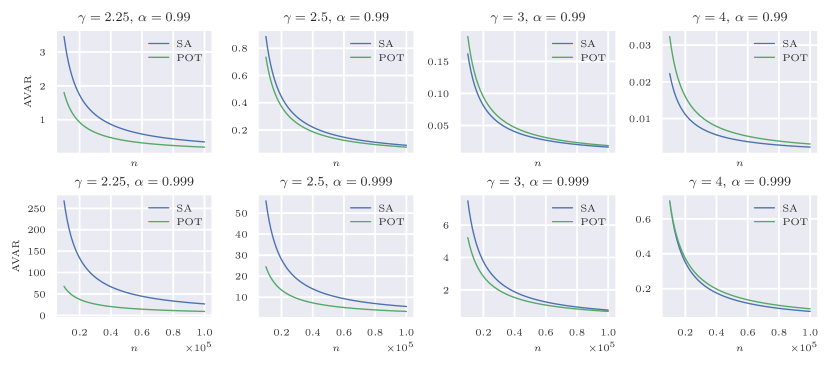
Figure 1: Asymptotic variance of the SA CVaR estimator (blue) and unbiased POT estimator (green) for the Fréchet($\gamma$) distribution at $\alpha=0.99,\,0.999$.

7.2 Error Analysis of CVaR Estimators

In the experiments that follow, samples are generated from the Burr, Fréchet, and half-$t$ distributions, which provide a good characterization of heavy-tailed phenomena with finite mean. Relevant details for each distribution class are provided in appendix C. The estimation performance of SA, BPOT, and UPOT are compared via the root-mean-square error (RMSE) and absolute bias on five examples from each distribution class, shown in fig. 2. We fix $\alpha=0.998$ as an example of an extreme risk level. Experiments are conducted as follows. Generate $N=1000$ random samples of size $50000$ from each distribution. For each sample, the CVaR is estimated using the three methods at subsample sizes $n=5000,10000,\ldots,50000$. In practice, it can be difficult to choose the number of threshold excesses $k$, and so we apply the ordered goodness-of-fits tests of Bader et al., (2018) to choose the optimal threshold. This threshold selection procedure, which we employ in both BPOT and UPOT, is given in detail in section B.2. The average threshold selected (in terms of the percentile of a given sample) was between 0.80 and 0.96 in all simulations performed. The complete algorithm for UPOT is summarized in section B.3.

Discussion. The chosen Burr distributions allow us to investigate the effect of varying $\rho$ while keeping a fixed $\xi$. In this case, we set $\xi=2/3$ while $\rho=-0.25,-0.33,-0.44,-1.33,-2.22$ in the respective Burr distributions. In general, when $\rho$ approaches $0$, the distribution’s tail deviates more severely from a strict Pareto model, and therefore we see the largest bias and RMSE occur in BPOT in the Burr(0.38, 4) and Burr(0.5, 3) models, while the bias-correction of UPOT leads to the most substantial performance gain. As a non-parametric estimator, SA is less affected by changes in the value of $\rho$, outperforming the POT estimators in terms of bias on some Burr distributions. However, as alluded to in section 7.1, high values of $\xi$ leads to high variance in observations, typically causing poor performance of SA in terms of RMSE. This effect is similarly observed in the Fréchet simulations, where SA has relatively low bias. The Fréchet distribution always has $\rho=-1$, a property shared with the GPD, giving its tail a similar shape. Therefore, the bias-correction of UPOT is less significant, but still provides a noticeable performance gain over BPOT. The results of the half-$t$ simulations are similar to the Fréchet, but we note a larger bias in BPOT due to the fact that the half-$t$ distribution has a $\rho$ value that varies with its parameter. Like in the Burr simulations, SA is unaffected by different values of $\rho$ and obtains good performance in terms of bias in the half-$t$ simulations, except when $\xi$ is largest in the half-$t$(1.5) model. Finally, we note that UPOT consistently had the lowest RMSE in all simulations except in a few cases at a sample size of $5000$. Next, the finite sample performance of the UPOT confidence interval is investigated.

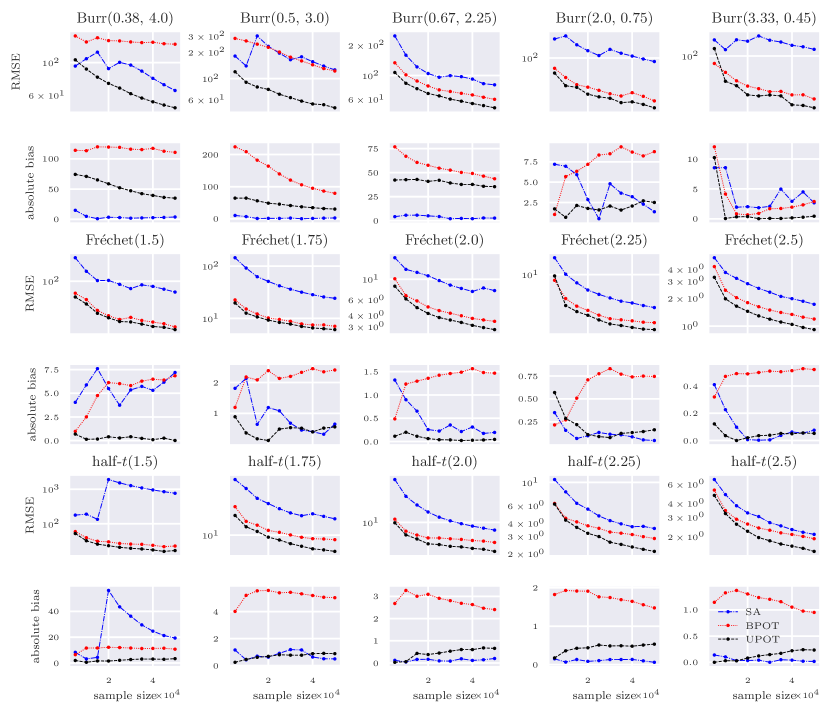
Figure 2: RMSE of and absolute bias of estimating CVaR_0.998 using UPOT (black), BPOT (red), and SA (blue).

7.3 Coverage Probability of the Asymptotic Confidence Interval

The accuracy of the confidence interval given in eq. 20 is assessed by its empirical coverage probability for each distribution using the same simulated data from section 7.2. Let $C^{n}_{i,\delta}$ denote the confidence interval computed for a sample of size $n$ for sample $i$, $i=1,\ldots,N$. Then, the empirical coverage probability is defined as

$$\hat{P}_{\delta}^{n}(N)=\frac{1}{N}\sum_{i=1}^{N}\mathds{1}_{\left\{c_{\alpha}\in C^{n}_{i,\delta}\right\}}.$$

Plots of the coverage probability at each sample size for each distribution are shown in fig. 3. We set $\delta=0.05$ and compute the coverage probability at sample sizes $n=5000,10000,\ldots,50000$. The final value of each distribution’s coverage probability at $n=50000$ is reported in appendix D. Most of the distributions tested achieve nearly the correct coverage of 0.95, sometimes surpassing it in some cases, and this is due to the estimated confidence interval being wider than its true asymptotic counterpart. The coverage is worst in the Burr(0.38, 4) distribution, achieving a final coverage probability of just 0.73. The small magnitude of $\rho$ in this distribution causes slow convergence of the tail to the GPD, and hence a relatively high average threshold percentile of 0.96 was chosen by the threshold selection procedure. This high threshold increases the variance of parameter estimation which explains the poor coverage.

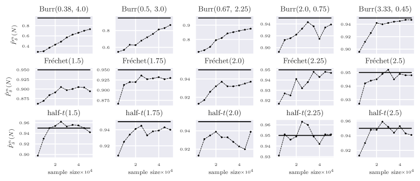
Figure 3: Coverage probabilities with $\alpha=0.998,\delta=0.05$. The solid line indicates the theoretical coverage, i.e., $1-\delta=0.95$.

8 Conclusion

We have studied the asymptotic properties of a new CVaR estimator based on the peaks-over-threshold approach. Using extreme value theory and second-order regular variation, we derived estimators for the bias induced by the approximate GPD model of the threshold excesses and the bias from maximum likelihood estimators of the GPD parameters. Using these results, we proved that our estimator is asymptotically normal and unbiased (up to some technical conditions). This convergence result allowed us to derive confidence intervals for the CVaR, enabling us to measure the level of uncertainty in our estimator. We compared the magnitudes of the asymptotic variance of our CVaR estimator with that of the sample average CVaR estimator, demonstrating a significant improvement in asymptotic performance for some cases. An empirical study showed that our CVaR estimator can lead to a significant performance improvement in heavy-tailed distributions when compared to the sample average estimator and the existing peaks-over-threshold estimator. Finally, we investigated the finite-sample performance of the asymptotic confidence interval, and found that good coverage probability is achieved in reasonable sample sizes. While our evidence suggests that our CVaR estimator is most effective in the heavy-tailed domain, it would also be instructive to perform the same theoretical analysis for light-tailed distributions. Doing so would allow our CVaR estimator to be robust to situations where it is not possible to make any assumptions about the underlying data distribution.

Appendix A Proofs

We first recall the stochastic order notation (e.g., Vaart, (1998, Section 2.2)), which will be used throughout subsequent proofs.

Definition A.1 (Stochastic $o$ and $O$ symbols).

Let $X_{n},R_{n}$ denote sequences of random variables. Then,

$$X_{n} =o_{p}(R_{n})\quad\textnormal{ means }\quad\forall\varepsilon>0,\,\lim_{n\to\infty}\mathbb{P}(|X_{n}/R_{n}|>\varepsilon)=0,$$

$$X_{n} =O_{p}(R_{n})\quad\textnormal{ means }\quad\forall\varepsilon>0,\,\exists M,N>0,\,\forall n>N,\,\mathbb{P}(|X_{n}/R_{n}|>M)<\varepsilon.$$

The often used notation $X_{n}=o_{p}(1)$ means that $X_{n}$ converges to zero in probability, and $X_{n}=O_{p}(1)$ means that $X_{n}$ is bounded in probability.

A.1 Proof of Theorem 3.1

We first state the following lemma, which is equivalent to Beirlant et al., (2003, Proposition 1) with different notation.

Lemma A.1.

Suppose assumption 2.1 and assumption 2.2 hold. Then $\forall\varepsilon>0,\;\exists t_{0},\;\forall t,x$ such that $t\geq t_{0}$ and $tx\geq t_{0}$,

$$(1-\varepsilon)e^{-\varepsilon|\log x|}\leq\left[\frac{U(tx)-U(t)}{a(t)}-\frac{x^{\xi}-1}{\xi}\right]/\left[A\left({t}\right)I_{\xi,\rho}(x)\right]\leq(1+\varepsilon)e^{\varepsilon|\log x|},$$ (23)

where

$$A(t)=\frac{tU^{\prime\prime}(t)}{U^{\prime}(t)}-\xi+1\quad\textnormal{ and }\quad I_{\xi,\rho}(x)=\begin{cases}\frac{1}{\rho}\left(\frac{x^{\xi+\rho}-1}{\xi+\rho}-\frac{x^{\xi}-1}{\xi}\right),\quad\rho<0,\,\xi+\rho\neq 0,\\ \frac{1}{\rho}\left(\log{x}-\frac{x^{\xi}-1}{\xi}\right),\quad\;\;\;\,\rho<0,\,\xi+\rho=0,\\ \frac{1}{\xi}\left(x^{\xi}\log{x}-\frac{x^{\xi}-1}{\xi}\right),\;\;\;\rho=0.\end{cases}$$

Proof.

In Beirlant et al., (2003), the statement is given as $\forall\varepsilon>0,\;\exists t_{0},\;\forall t,x$ such that $t\geq t_{0}$ and $t+x\geq t_{0}$,

$$(1-\varepsilon)e^{-\varepsilon|x|}\leq\left[\frac{V(t+x)-V(t)}{V^{\prime}(t)}-\frac{e^{\xi x}-1}{\xi}\right]/\left[\tilde{A}\left(e^{t}\right)\tilde{I}_{\xi,\rho}(x)\right]\leq(1+\varepsilon)e^{\varepsilon|x|},$$ (24)

where

$$V(t)=(\bar{F})^{-1}\left(e^{-t}\right),\qquad\tilde{A}(t)=\frac{V^{\prime\prime}(\log t)}{V^{\prime}(\log t)}-\xi,\qquad\tilde{I}_{\xi,\rho}(x)=I_{\xi,\rho}(e^{x}).$$

Then, for $t\geq 1$,

$$V(\log t)=(\bar{F})^{-1}(1/t)=(1/\bar{F})^{-1}(t)=U(t),$$

and

$$V^{\prime}(\log t)=tU^{\prime}(t)=a(t),\quad V^{\prime\prime}(\log t)=t^{2}U^{\prime\prime}(t)+tU^{\prime}(t)\quad\Rightarrow\quad\tilde{A}(t)=A(t).$$

Since $\log$ is strictly increasing, eq. 24 holds with $\log t$ and $\log x$ where $\log t\geq t_{0}$ and $\log tx\geq t_{0}$. Substituting expressions in eq. 24, we get eq. 23. ∎

The following corollary will also be used in the main proof of this section.

Corollary A.1.

An immediate consequence of lemma A.1 is for all $x>0,$

$$\lim_{t\rightarrow\infty}\frac{\frac{U(tx)-U(t)}{a(t)}-\frac{x^{\xi}-1}{\xi}}{A(t)}=I_{\xi,\rho}(x).$$ (25)

corollary A.1 can also be found in De Haan and Ferreira, (2006, Theorem 2.3.12). Before proving our main result of this section, we first recall the dominated convergence theorem which will be needed later.

Theorem A.1 (Dominated convergence theorem).

Let $\{f_{n}\}_{n=1}^{\infty}$ be a sequence of real-valued functions defined on $S\subset\mathbb{R}$ such that $\forall x\in S,\,\lim_{n\to\infty}f_{n}(x)\to f(x)$. If $\forall x\in S,\,n,$

$$|f_{n}(x)|\leq g(x)$$

for some integrable (i.e., the integral is finite over $S$) function $g$, then

$$\lim_{n\to\infty}\int_{S}f_{n}(x)dx=\int_{S}\lim_{n\to\infty}f_{n}(x)dx=\int_{S}f(x)dx.$$

Proof of Theorem 3.1. We use corollary A.1 to derive a convergence result for the approximation error of the VaR, i.e, $q_{\alpha}-q_{u,\alpha}$. Then, using lemma A.1 and theorem A.1, we will be able to derive the convergence of $\epsilon_{u,\alpha}$.

For any $p\in(0,1)$ and $y\in\operatorname*{dom}F$ such that $F(y)=p$,

$$\left(\frac{1}{\bar{F}}\right)(y)=\frac{1}{\bar{F}(y)}=\frac{1}{1-p},$$

which implies that

$$U\left(\frac{1}{1-p}\right)=\left(\frac{1}{\bar{F}}\right)^{-1}(1/(1-p))=y.$$

Hence,

$$U(1/(1-\alpha))=U(\tau_{u}\beta)=q_{\alpha}\quad\textnormal{ and }\quad U(\tau_{u})=u.$$

Then, from the definition of $q_{u,\alpha}$ we get

$$q_{u,\alpha}=u+\frac{\sigma(u)}{\xi}\left(\beta^{\xi}-1\right)=U(\tau_{u})+\frac{a(\tau_{u})}{\xi}(\beta^{\xi}-1).$$

Setting $D_{u}(\beta)=(q_{\alpha}-q_{u,\alpha})/(a(\tau_{u})A(\tau_{u}))$, it then follows from the previous two equations and corollary A.1 with $t=\tau_{u}$, $x=\beta$ that

$$D_{u}(\beta)=\frac{U(\tau_{u}\beta)-U(\tau_{u})-\frac{a(\tau_{u})}{\xi}(\beta^{\xi}-1)}{a(\tau_{u})A(\tau_{u})}=\frac{\frac{U(\tau_{u}\beta)-U(\tau_{u})}{a(\tau_{u})}-\frac{\beta^{\xi}-1}{\xi}}{A(\tau_{u})}\to I_{\xi,\rho}(\beta)\quad\textnormal{ as }u\to\infty.$$ (26)

From the definition of the GPD approximation error and the CVaR, for a fixed $u,\alpha$,

$$\frac{\epsilon_{u,\alpha}}{a(\tau_{u})A(\tau_{u})}=\frac{c_{u,\alpha}-c_{\alpha}}{a(\tau_{u})A(\tau_{u})}=-\frac{1}{1-\alpha}\int_{\alpha}^{1}\frac{q_{\gamma}-q_{u,\gamma}}{a(\tau_{u})A(\tau_{u})}d\gamma=-\beta\int_{\beta}^{\infty}\frac{D_{u}(x)}{x^{2}}dx,$$ (27)

where $D_{u}(x)=(q_{\gamma}-q_{u,\gamma})/(a(\tau_{u})A(\tau_{u}))$ and we have used the substitution $x=\bar{F}(u)/(1-\gamma)$. We now apply the dominated convergence theorem to get the limiting behaviour of eq. 27 as $u\to\infty$. From lemma A.1, $\forall\varepsilon>0,\,\exists u_{0}$ such that $\forall u\geq u_{0},\,x\in[\beta,\infty)$,

$$\left|\frac{D_{u}(x)}{x^{2}}\right|\leq(1+\varepsilon)x^{\varepsilon-2}I_{\xi,\rho}(x).$$

$(1+\varepsilon)x^{\varepsilon-2}I_{\xi,\rho}(x)$ is integrable over $[\beta,\infty)$ as long as $\varepsilon<1-\xi$. Since $\xi<1$, let $\varepsilon=(1-\xi)/2$. Then theorem A.1 can be applied to $D_{u}(x)/x^{2}$. Setting $K_{\xi,\rho}(\beta)=-\beta\int_{\beta}^{\infty}[I_{\xi,\rho}(x)/x^{2}]dx$, it follows that

$$\lim_{u\to\infty}\frac{\epsilon_{u,\alpha}}{a(\tau_{u})A(\tau_{u})} =\lim_{u\to\infty}-\beta\int_{\beta}^{\infty}\frac{D_{u}(x)}{x^{2}}dx$$

$$=-\beta\int_{\beta}^{\infty}\lim_{u\to\infty}\frac{D_{u}(x)}{x^{2}}dx$$

$$=-\beta\int_{\beta}^{\infty}\frac{I_{\xi,\rho}(x)}{x^{2}}dx$$

$$=K_{\xi,\rho}(\beta),$$

where the last integral can be computed explicitly to obtain eq. 9. ∎

A.2 Proof of Theorem 4.2

First recall Slutsky’s lemma (see, for example, Vaart, (1998, Lemma 2.8)).

Lemma A.2 (Slutsky).

Let $X_{n},\,X,\,Y_{n}$ be random vectors or variables. If $X_{n}\overset{d}{\to}X$ and $Y_{n}\overset{p}{\to}c$ for a constant $c$, then

1. $X_{n}+Y_{n}\overset{d}{\to}X+c$;

2. $X_{n}Y_{n}\overset{d}{\to}Xc$;

3. $X_{n}/Y_{n}\overset{d}{\to}X/c$ provided $c\neq 0.$

Proof of Theorem 4.2. First note that since $\hat{A}_{n}$ and $\hat{b}_{n}$ are consistent, i.e.,

$$\frac{\hat{A}_{n}}{A(n/k)}\overset{p}{\to}1,\qquad\hat{b}_{n}\overset{p}{\to}b_{\xi,\rho},$$

then by lemma A.2, the fact that $\hat{\sigma}^{\scriptscriptstyle{(n)}}_{\scriptscriptstyle{\textnormal{MLE}}}/a(n/k)\overset{p}{\to}1$ (which follows from theorem 4.1), and the assumption of theorem 4.1 that $\lim_{n\to\infty}\sqrt{k}A(n/k)\to\lambda<\infty$,

$$\sqrt{k}\hat{A}_{n}\left(\hat{b}^{(1)}_{n},\;\frac{\hat{\sigma}^{\scriptscriptstyle{(n)}}_{\scriptscriptstyle{\textnormal{MLE}}}}{a(n/k)}\hat{b}^{(2)}_{n}\right) =\sqrt{k}A(n/k)\frac{\hat{A}_{n}}{A(n/k)}\left(\hat{b}^{(1)}_{n},\;\frac{\hat{\sigma}^{\scriptscriptstyle{(n)}}_{\scriptscriptstyle{\textnormal{MLE}}}}{a(n/k)}\hat{b}^{(2)}_{n}\right)$$

$$\overset{p}{\to}\lambda\left(b_{\xi,\rho}^{(1)},\;b_{\xi,\rho}^{(2)}\right)$$

$$=\lambda b_{\xi,\rho}.$$

Then, by expanding terms and applying lemma A.2 once again,

$$\sqrt{k}(\hat{\xi}_{n}-\xi,\;\hat{\sigma}_{n}/a(n/k)-1) =\sqrt{k}(\hat{\xi}^{\scriptscriptstyle{(n)}}_{\scriptscriptstyle{\textnormal{MLE}}}-\hat{A}_{n}\hat{b}^{(1)}_{n}-\xi,\;\hat{\sigma}^{\scriptscriptstyle{(n)}}_{\scriptscriptstyle{\textnormal{MLE}}}(1-\hat{A}_{n}\hat{b}^{(2)}_{n})/a(n/k)-1)$$

$$=\sqrt{k}(\hat{\xi}^{\scriptscriptstyle{(n)}}_{\scriptscriptstyle{\textnormal{MLE}}}-\xi,\;\hat{\sigma}^{\scriptscriptstyle{(n)}}_{\scriptscriptstyle{\textnormal{MLE}}}/a(n/k)-1)-\sqrt{k}\hat{A}_{n}\left(\hat{b}^{(1)}_{n},\;\frac{\hat{\sigma}^{\scriptscriptstyle{(n)}}_{\scriptscriptstyle{\textnormal{MLE}}}}{a(n/k)}\hat{b}^{(2)}_{n}\right)$$

$$\overset{d}{\to}N(\lambda b_{\xi,\rho},\mathbf{\Sigma})-\lambda b_{\xi,\rho}$$

$$=N(0,\mathbf{\Sigma}).$$

∎

A.3 Proof of Theorem 4.3

We first give the delta method, which can be found in, for example, Rémillard, (2016, Appendix B.3.4.1).

Theorem A.2 (Delta method).

Let $\hat{\theta}_{n}\in\mathbb{R}^{m}$ be a random vector based on a sample of size $n$. Suppose that $h:\mathbb{R}^{m}\mapsto\mathbb{R}$ is such that for $i=1,\ldots,m$, $\frac{\partial h}{\partial\theta_{i}}$ exists and is continuous in a neighborhood of $\theta$. If $\sqrt{n}(\hat{\theta}_{n}-\theta)\overset{d}{\to}N(0,V)$, then

$$\sqrt{n}(h(\hat{\theta}_{n})-h(\theta))\overset{d}{\to}N(0,\nabla h(\theta)^{\top}V\nabla h(\theta)),$$

where $\nabla h(\theta)$ is the gradient of $h$ evaluated at $\theta$.

Next, we prove some useful lemmas which will be used in the proof of theorem 4.3.

Lemma A.3.

Let $X_{1},\ldots,X_{n}$ be an i.i.d. sample with common cdf $F$, and suppose $k=k_{n}\to\infty$ and $k/n\to 0$ as $n\to\infty$. With $u=X_{(n-k,n)}$ and $\xi\in\mathbb{R}$,

$$\sqrt{k}\left((k\tau_{u}/n)^{\xi}-1\right)\overset{d}{\to}N(0,\xi^{2}).$$

Proof.

Letting $h_{\xi}(x)=x^{-\xi},$

$$\sqrt{k}\left((k\tau_{u}/n)^{\xi}-1\right)=\sqrt{k}\left((n\bar{F}(u)/k)^{-\xi}-1\right)=\sqrt{k}\left(h_{\xi}(n\bar{F}(u)/k)-h_{\xi}(1)\right).$$

From Beirlant et al., (2009, Theorem 3.1), we know that $\sqrt{k}(n\bar{F}(u)/k-1)\overset{d}{\to}N(0,1).$ Hence, by theorem A.2,

$$\sqrt{k}\left((k\tau_{u}/n)^{\xi}-1\right)\overset{d}{\to}N(0,h_{\xi}^{\prime}(1)\cdot 1\cdot h_{\xi}^{\prime}(1))=N(0,\xi^{2}).$$

∎

Corollary A.2.

Let $\alpha=\alpha_{n}=1-(1/\beta)k/n$ where $\beta>1$ is a constant not depending on $n$. Then,

$$\sqrt{k}(s_{u,\alpha}^{\xi}-\beta^{\xi})\overset{d}{\to}N(0,\xi^{2}\beta^{2\xi}).$$

Proof.

$$s_{u,\alpha}=\bar{F}(u)\left(\frac{n}{k}\right)\frac{k}{n(1-\alpha)}=\beta n\bar{F}(u)/k=\frac{\beta n}{k\tau_{u}},$$

and so

$$\sqrt{k}(s_{u,\alpha}^{\xi}-\beta^{\xi})=\beta^{\xi}\sqrt{k}((k\tau_{u}/n)^{-\xi}-1)=-\beta^{\xi}(n\bar{F}(u)/k)^{\xi}\sqrt{k}((k\tau_{u}/n)^{\xi}-1).$$ (28)

Beirlant et al., (2009, Theorem 3.1) implies that $n\bar{F}(u)/k\overset{p}{\to}1$. Hence, lemma A.3 with eq. 28 implies

$$\sqrt{k}(s_{u,\alpha}^{\xi}-\beta^{\xi})\overset{d}{\to}N(0,\xi^{2}\beta^{2\xi}).$$

∎

Lemma A.4.

Suppose that the assumptions of theorem 4.1 hold. Then as $n\to\infty$,

$$\sqrt{k}\left(\frac{a(\tau_{u})}{a(n/k)}-(k\tau_{u}/n)^{\xi}\right)=o_{p}(1).$$ (29)

Proof.

Under 2.1 and 2.2, the following uniform inequality from De Haan and Ferreira, (2006, Theorem 2.3.6) holds: for any $\varepsilon,\delta>0$ there exists $t_{0}=t_{0}(\varepsilon,\delta)$ such that for all $t,tx\geq t_{0}$,

$$\left|\frac{\frac{a(tx)}{a(t)}-x^{\xi}}{A(t)}-x^{\xi}\frac{x^{\rho}-1}{\rho}\right|\leq\varepsilon x^{\xi+\rho}\max\left(x^{\delta},x^{-\delta}\right).$$ (30)

Hence, with $t=n/k$ and $x=k\tau_{u}/n$, for any $\varepsilon,\delta>0$ and with large enough $n$,

$$\sqrt{k}\left(\frac{a(\tau_{u})}{a(n/k)}-(k\tau_{u}/n)^{\xi}\right) =\sqrt{k}A(n/k)\left[\frac{\frac{a(\tau_{u})}{a(n/k)}-(k\tau_{u}/n)^{\xi}}{A(n/k)}-(k\tau_{u}/n)^{\xi}\frac{(k\tau_{u}/n)^{\rho}-1}{\rho}\right]$$

$$\qquad+\sqrt{k}A(n/k)(k\tau_{u}/n)^{\xi}\frac{(k\tau_{u}/n)^{\rho}-1}{\rho}$$

$$\leq\sqrt{k}A(n/k)\left|\frac{\frac{a(\tau_{u})}{a(n/k)}-(k\tau_{u}/n)^{\xi}}{A(n/k)}-(k\tau_{u}/n)^{\xi}\frac{(k\tau_{u}/n)^{\rho}-1}{\rho}\right|$$

$$\qquad+\sqrt{k}A(n/k)(k\tau_{u}/n)^{\xi}\frac{(k\tau_{u}/n)^{\rho}-1}{\rho}$$

$$\leq\sqrt{k}A(n/k)\varepsilon(k\tau_{u}/n)^{\xi+\rho}\max\left((k\tau_{u}/n)^{\delta},(k\tau_{u}/n)^{-\delta}\right)$$

$$\qquad+\sqrt{k}A(n/k)(k\tau_{u}/n)^{\xi}\frac{(k\tau_{u}/n)^{\rho}-1}{\rho}.$$

Since $k\tau_{u}/n\overset{p}{\to}1$ and $\sqrt{k}A(n/k)\to\lambda<\infty$ as $n\to\infty$ (by the assumption of theorem 4.1), and since $\varepsilon$ can be made arbitrarily small as $n\to\infty$, both terms tend to $0$ in probability as $n\to\infty,$ hence eq. 29 follows. ∎

The following corollary is an immediate result by combining lemma A.3 and lemma A.4.

Corollary A.3.

Suppose that the assumptions of theorem 4.1 hold. Then,

$$\sqrt{k}\left(\frac{a(\tau_{u})}{a(n/k)}-1\right)\overset{d}{\to}N(0,\xi^{2}).$$

Proof of Theorem 4.3. With $\alpha=1-(1/\beta)k/n$ and $u=X_{(n-k,n)}$,

$$\frac{\hat{c}^{(n)}_{\alpha}}{a(n/k)}=\frac{\hat{\sigma}_{n}/a(n/k)}{1-\hat{\xi}_{n}}\left(1+\frac{\beta^{\hat{\xi}_{n}}-1}{\hat{\xi}_{n}}\right)+\frac{u}{a(n/k)}=d_{\beta}(\hat{\xi}_{n},\hat{\sigma}_{n}/a(n/k))+\frac{u}{a(n/k)},$$

and recalling that $s_{u,\alpha}=\bar{F}(u)/(1-\alpha)$,

$$\frac{c_{u,\alpha}}{a(n/k)} =\frac{\sigma(u)/a(n/k)}{1-{\xi}}\left(1+\frac{s_{u,\alpha}^{{\xi}}-1}{{\xi}}\right)+\frac{u}{a(n/k)}$$

$$=\frac{1}{1-{\xi}}\left(1+\frac{s_{u,\alpha}^{{\xi}}-1}{{\xi}}\right)+\frac{\sigma(u)/a(n/k)-1}{1-{\xi}}\left(1+\frac{s_{u,\alpha}^{{\xi}}-1}{{\xi}}\right)+\frac{u}{a(n/k)}.$$

Then for the first term,

$$\frac{1}{1-{\xi}}\left(1+\frac{s_{u,\alpha}^{{\xi}}-1}{{\xi}}\right) =\frac{1}{1-{\xi}}\left(1+\frac{s_{u,\alpha}^{{\xi}}-1+\beta^{\xi}-\beta^{\xi}}{{\xi}}\right)$$

$$=\frac{1}{1-{\xi}}\left(1+\frac{\beta^{\xi}-1}{{\xi}}+\frac{s_{u,\alpha}^{{\xi}}-\beta^{\xi}}{{\xi}}\right)$$

$$=d_{\beta}(\xi,1)+\frac{s_{u,\alpha}^{{\xi}}-\beta^{\xi}}{\xi(1-\xi)}.$$

Recalling that $\sigma(u)=a(\tau_{u})$ and combining the previous expressions,

$$\frac{\sqrt{k}}{a(n/k)}\left(\hat{c}^{(n)}_{\alpha}-c_{u,\alpha}\right)=\sqrt{k}\left(d_{\beta}(\hat{\xi}_{n},\hat{\sigma}_{n}/a(n/k))-d_{\beta}(\xi,1)\right)\\ -\sqrt{k}\left(\frac{a(\tau_{u})/a(n/k)-1}{1-{\xi}}\left(1+\frac{s_{u,\alpha}^{{\xi}}-1}{{\xi}}\right)+\frac{s_{u,\alpha}^{{\xi}}-\beta^{\xi}}{\xi(1-\xi)}\right)=S-R,$$ (31)

where we have denoted each term by $S$ and $R$, respectively. By the delta method (theorem A.2),

$$S\overset{d}{\to}N(0,\nabla d_{\beta}(\xi,1)^{\top}\mathbf{\Sigma}\nabla d_{\beta}(\xi,1)).$$

For the second term, let

$$P=\sqrt{k}\left(\frac{a(\tau_{u})}{a(n/k)}-(k\tau_{u}/n)^{\xi}\right)\quad\textnormal{ and }\quad Q=\sqrt{k}\left((k\tau_{u}/n)^{\xi}-1\right).$$

Then $\sqrt{k}(a(\tau_{u})/a(n/k)-1)=P+Q$ and from eq. 28, $\sqrt{k}(s_{u,\alpha}^{\xi}-\beta^{\xi})=-s_{u,\alpha}^{\xi}Q$. Hence,

$$R=\frac{1}{\xi(1-\xi)}\left[(P+Q)(\xi+s_{u,\alpha}^{\xi}-1)-s_{u,\alpha}^{\xi}Q\right]=\frac{(\xi+s_{u,\alpha}^{\xi}-1)}{\xi(1-\xi)}P-\frac{Q}{\xi}.$$

corollary A.2 implies that $s_{u,\alpha}^{\xi}=\beta^{\xi}+o_{p}(1)$ as $n\to\infty$ and from lemma A.4 we know that $P=o_{p}(1)$ as $n\to\infty.$ By lemma A.3, $Q\overset{d}{\to}N(0,\xi^{2})$, and so $R\overset{d}{\to}N(0,1).$ By the assumption that $(\hat{\xi}_{n},\hat{\sigma}_{n})$ and $Q$ are asymptotically independent, $R$ and $S$ are as well. Hence, eq. 31 implies

$$\frac{\sqrt{k}}{a(n/k)}\left(\hat{c}^{(n)}_{\alpha}-c_{u,\alpha}\right)\overset{d}{\to}N\left(0,\nabla d_{\beta}(\xi,1)^{\top}\mathbf{\Sigma}\nabla d_{\beta}(\xi,1)+1\right)=N(0,V),$$

where

$$\nabla d_{\beta}(\xi,1)=\left[\ \frac{\partial d_{\beta}}{\partial x}(\xi,1),\frac{\partial d_{\beta}}{\partial y}(\xi,1)\right]^{\top},$$

with

$$\frac{\partial d_{\beta}}{\partial x}(\xi,1)=\frac{\beta^{\xi}(2\xi+\xi(1-\xi)\log\beta-1)}{\xi^{2}(1-\xi)^{2}}+\frac{1}{\xi^{2}},\quad\frac{\partial d_{\beta}}{\partial y}(\xi,1)=\frac{\beta^{\xi}+\xi-1}{\xi(1-\xi)}.$$

∎

A.4 Proof of Theorem 5.1

We first prove the following lemma, which shows that when $\tau_{u}$ is replaced by $n/k$ in theorem 3.1, the asymptotic behaviour of $\epsilon_{u,\alpha}$ is the same (in probability).

Lemma A.5.

Suppose that the assumptions of theorem 4.1 hold. Let $\alpha=1-(1/\beta)k/n$ where $\beta>1$ is a constant not depending on $n$. Then,

$$\frac{\epsilon_{u,\alpha}}{a(n/k)A(n/k)K_{\xi,\rho}(\beta)}\overset{p}{\to}1.$$

Proof.

We follow the same line of reasoning as in the proof of theorem 3.1. First, we have

$$q_{u,\alpha} =u+\frac{\sigma(u)}{\xi}(s_{u,\alpha}^{\xi}-1)$$

$$=U(\tau_{u})+\frac{a(\tau_{u})}{\xi}(s_{u,\alpha}^{\xi}-1)$$

$$=U(n/k)+\frac{a(n/k)}{\xi}(\beta^{\xi}-1)+U(\tau_{u})-U(n/k)+\frac{1}{\xi}\left[a(\tau_{u})(s_{u,\alpha}^{\xi}-1)-a(n/k)(\beta^{\xi}-1)\right]$$

$$=U(n/k)+\frac{a(n/k)}{\xi}(\beta^{\xi}-1)+U(\tau_{u})-U(n/k)$$

$$\qquad\qquad\qquad\qquad\qquad\qquad\;\;+\frac{1}{\xi}\left[a(\tau_{u})(s_{u,\alpha}^{\xi}-\beta^{\xi})+(a(\tau_{u})-a(n/k))(\beta^{\xi}-1)\right].$$

Given that $q_{\alpha}=U(1/(1-\alpha))=U(n\beta/k)$,

$$\frac{q_{\alpha}-q_{u,\alpha}}{a(n/k)A(n/k)} =\frac{\frac{U(n\beta/k)-U(n/k)}{a(n/k)}-\frac{\beta^{\xi}-1}{\xi}}{A(n/k)}$$

$$\quad-\frac{U(\tau_{u})-U(n/k)}{a(n/k)A(n/k)}-\frac{a(\tau_{u})(s_{u,\alpha}^{\xi}-\beta^{\xi})}{\xi a(n/k)A(n/k)}-\left(\frac{a(\tau_{u})}{a(n/k)}-1\right)\frac{\beta^{\xi}-1}{\xi A(n/k)}$$

$$=I-II-III-IV.$$

In what follows, terms $I$-$IV$ will be analyzed separately then finally combined.

$I$: By corollary A.1, with $t=n/k$ and $x=\beta$ we know that term $I$ tends to $I_{\xi,\rho}(\beta)$ as $n\to\infty.$

$II$: Under 2.1 and 2.2, the following uniform inequality from De Haan and Ferreira, (2006, Theorem 2.3.6) holds: for any $\varepsilon,\delta>0$ there exists $t_{0}=t_{0}(\varepsilon,\delta)$ such that for all $t,tx\geq t_{0}$,

$$\left|\frac{\frac{U(tx)-U(t)}{a(t)}-\frac{x^{\xi}-1}{\xi}}{A(t)}-\frac{x^{\xi+\rho}-1}{\xi+\rho}\right|\leq\varepsilon x^{\xi+\rho}\max\left(x^{\delta},x^{-\delta}\right).$$ (32)

We can write $II$ as

$$II=\frac{\frac{U(\tau_{u})-U(n/k)}{a(n/k)}-\frac{(k\tau_{u}/n)^{\xi}-1}{\xi}}{A(n/k)}+\frac{(k\tau_{u}/n)^{\xi}-1}{\xi A(n/k)}.$$

Hence, with $t=n/k$ and $x=k\tau_{u}/n$, the first term tends to $0$ in probability using eq. 32 and essentially the same arguments as in the proof of lemma A.4. So, by the assumption of theorem 4.1 that $\sqrt{k}A(n/k)\to\lambda<\infty$ as $n\to\infty$ and lemma A.3,

$$II=\frac{Q}{\xi\sqrt{k}A(n/k)}+o_{p}(1)=\frac{Z}{\lambda}+o_{p}(1),\quad n\to\infty,$$

where $Q=\sqrt{k}((k\tau_{u}/n)^{\xi}-1)$ and $Z$ denotes a standard normal random variable.

$III$: corollary A.3 implies that $a(\tau_{u})/a(n/k)\overset{p}{\to}1$ and by eq. 28, $s_{u,\alpha}^{\xi}-\beta^{\xi}=-s_{u,\alpha}^{\xi}Q/\sqrt{k}$. Corollary A.2 implies that $s_{u,\alpha}^{\xi}\overset{p}{\to}\beta^{\xi}$, and so

$$III=\frac{a(\tau_{u})(s_{u,\alpha}^{\xi}-\beta^{\xi})}{\xi a(n/k)A(n/k)}=\frac{-s_{u,\alpha}^{\xi}Q}{\xi\sqrt{k}A(n/k)}(1+o_{p}(1))=-\frac{\beta^{\xi}}{\lambda}Z+o_{p}(1),\quad n\to\infty.$$

$IV$: With $P=\sqrt{k}\left(\frac{a(\tau_{u})}{a(n/k)}-(k\tau_{u}/n)^{\xi}\right)$ and applying lemma A.4,

$$IV=\left(\frac{a(\tau_{u})}{a(n/k)}-1\right)\frac{\beta^{\xi}-1}{\xi A(n/k)}=(P+Q)\frac{\beta^{\xi}-1}{\xi\sqrt{k}A(n/k)}=\frac{\beta^{\xi}-1}{\lambda}Z+o_{p}(1),\quad n\to\infty.$$

Now combining all terms, as $n\to\infty$,

$$\frac{q_{\alpha}-q_{u,\alpha}}{a(n/k)A(n/k)}=I-II-III-IV\\ =I_{\xi,\rho}(\beta)-\frac{Z}{\lambda}+\frac{\beta^{\xi}}{\lambda}Z-\frac{\beta^{\xi}-1}{\lambda}Z+o_{p}(1)=I_{\xi,\rho}(\beta)+o_{p}(1),\quad n\to\infty.$$

Hence, following the same reasoning as in the proof of theorem 3.1,

$$\frac{\epsilon_{u,\alpha}}{a(n/k)A(n/k)}=\frac{c_{u,\alpha}-c_{\alpha}}{a(n/k)A(n/k)}\\ =-\frac{1}{1-\alpha}\int_{\alpha}^{1}\frac{q_{\gamma}-q_{u,\gamma}}{a(n/k)A(n/k)}d\gamma\overset{p}{\to}-\beta\int_{\beta}^{\infty}\frac{I_{\xi,\rho}(x)}{x^{2}}dx=K_{\xi,\rho}(\beta).$$

∎

Proof of Theorem 5.1. First,

$$\hat{c}^{(n)}_{\epsilon,\alpha}-c_{\alpha}=\hat{c}^{(n)}_{\alpha}-\hat{\epsilon}^{(n)}_{\alpha}-c_{\alpha}=\hat{c}^{(n)}_{\alpha}-c_{u,\alpha}-\hat{\epsilon}^{(n)}_{\alpha}+c_{u,\alpha}-c_{\alpha}=\hat{c}^{(n)}_{\alpha}-c_{u,\alpha}-\hat{\epsilon}^{(n)}_{\alpha}+\epsilon_{u,\alpha}.$$

Hence,

$$\frac{\sqrt{k}(\hat{c}^{(n)}_{\epsilon,\alpha}-c_{\alpha})}{\hat{\sigma}_{n}}=\frac{\sqrt{k}(\hat{c}^{(n)}_{\alpha}-c_{u,\alpha})}{\hat{\sigma}_{n}}-\frac{\sqrt{k}(\hat{\epsilon}^{(n)}_{\alpha}-\epsilon_{u,\alpha})}{\hat{\sigma}_{n}}.$$ (33)

For the first term on the right-hand side of eq. 33,

$$\frac{\sqrt{k}(\hat{c}^{(n)}_{\alpha}-c_{u,\alpha})}{\hat{\sigma}_{n}}=\frac{a(n/k)}{\hat{\sigma}_{n}}\frac{\sqrt{k}(\hat{c}^{(n)}_{\alpha}-c_{u,\alpha})}{a(n/k)}\overset{d}{\to}N(0,V),$$ (34)

which follows from theorem 4.3 and applying lemma A.2 with the fact that $\hat{\sigma}_{n}/a(n/k)\overset{p}{\to}1$.

For the second term, first recall that

$$\frac{\hat{\epsilon}^{(n)}_{\alpha}}{a(n/k)A(n/k)}=\frac{\hat{\sigma}_{n}\hat{A}_{n}\hat{K}_{n}}{a(n/k)A(n/k)}\overset{p}{\to}K_{\xi,\rho}(\beta),$$

which follows from lemma A.2 and the continuous mapping theorem. Then, under the assumption that $\sqrt{k}A(n/k)\to\lambda<\infty$ ($n\to\infty$), it follows from lemma A.2 and lemma A.5 that

$$\frac{\sqrt{k}(\hat{\epsilon}^{(n)}_{\alpha}-\epsilon_{u,\alpha})}{\hat{\sigma}_{n}}=\frac{a(n/k)\sqrt{k}A(n/k)}{\hat{\sigma}_{n}}\left(\frac{\hat{\epsilon}^{(n)}_{\alpha}-\epsilon_{u,\alpha}}{a(n/k)A(n/k)}\right)\\ =\lambda(1+o_{p}(1))\left(K_{\xi,\rho}(\beta)-K_{\xi,\rho}(\beta)+o_{p}(1)\right)=o_{p}(1),\quad n\to\infty.$$ (35)

Combining the convergence in eq. 34 and eq. 35 with eq. 33, it follows that

$$\frac{\sqrt{k}(\hat{c}^{(n)}_{\epsilon,\alpha}-c_{\alpha})}{\hat{\sigma}_{n}}\overset{d}{\to}N(0,V),$$

and hence,

$$\frac{\sqrt{k}(\hat{c}^{(n)}_{\epsilon,\alpha}-c_{\alpha})}{\hat{\sigma}_{n}\sqrt{\hat{V}_{n}}}=\frac{\sqrt{k}(\hat{c}^{(n)}_{\epsilon,\alpha}-c_{\alpha})}{\hat{\sigma}_{n}\sqrt{V}}\frac{\sqrt{V}}{\sqrt{\hat{V}_{n}}}\overset{d}{\to}N(0,1),$$

which follows from the fact that $\hat{V}_{n}\overset{p}{\to}V$ (from the continuous mapping theorem) and lemma A.2. ∎

A.5 Consistency of A(n/k) Estimator

In Haouas et al., (2018), an estimator for $A_{0}(n/k)$ is given, where the function $A_{0}$ satisfies the second-order condition of De Haan and Ferreira, (2006, Theorem 2.3.9), where for all $x>0,$

$$\lim_{t\rightarrow\infty}\frac{\frac{U(tx)}{U(t)}-x^{\xi}}{A_{0}(t)}=x^{\xi}\frac{x^{\rho}-1}{\rho}.$$ (36)

Note that under 2.1 and 2.2, eq. 36 is satisfied. The relation between the function $A$ defined in eq. 7 and $A_{0}$ is given in De Haan and Ferreira, (2006, Table 3.1), where

$$A=\frac{\xi+\rho}{\xi}A_{0}.$$ (37)

We shall use this relation and an estimator for $A_{0}(n/k)$ to derive an estimator for $A(n/k)$. To prove consistency of the forthcoming estimator, we start with the following relation from Haouas et al., (2018):

$$\lim_{t\to\infty}\frac{A_{0}(t)}{R(t)}=1,$$ (38)

where

$$R(t)=\frac{(1-\rho^{2})(M^{(2)}(t)-2(M^{(1)}(t))^{2})}{2\rho M^{(1)}(t)},\quad M^{(j)}(t)=t\int_{U(t)}^{\infty}\log^{j}\left(x/U(t)\right)dF(x).$$

This leads to an estimator for $A_{0}(n/k)$ Haouas et al., (2018, p. 7),

$$\hat{A}_{0}^{(n)}=\frac{(1-\hat{\rho}_{n}^{2})(\hat{M}_{n}^{(2)}-2(\hat{M}_{n}^{(1)})^{2})}{2\hat{\rho}_{n}\hat{M}_{n}^{(1)}},$$

where $\hat{M}_{n}^{(j)}$ is an estimator for $M^{(j)}(n/k)$, given by

$$\hat{M}_{n}^{(j)}=\frac{1}{k}\sum_{i=1}^{k}[\log X_{(n-i+1,k)}-\log X_{(n-k,n)}]^{j},$$

which is also given in section 6.2. Note that $\hat{M}_{n}^{(1)}$ is the well-known Hill estimator of $\xi$. $\hat{M}_{n}^{(j)}$ is consistent for $j=1,2$ under the conditions of the following lemma.

Lemma A.6.

Suppose that 2.1 holds. If $k=k_{n}\to\infty,\,k/n\to 0$ as $n\to\infty$, then

$$\frac{\hat{M}_{n}^{(j)}}{M^{(j)}(n/k)}\overset{p}{\to}1,\qquad j=1,2.$$

Proof.

From Haouas et al., (2018, equation 1.9),

$$M^{(1)}(t)\to\xi\quad\textnormal{ and }\quad M^{(2)}(t)\to 2\xi^{2},\quad t\to\infty.$$

By De Haan and Ferreira, (2006, Theorem 3.2.2), $\hat{M}_{n}^{(1)}\overset{p}{\to}\xi$, and by De Haan and Ferreira, (2006, Equation 3.5.7), $\hat{M}_{n}^{(2)}\overset{p}{\to}2\xi^{2}$. Hence, by lemma A.2,

$$\frac{\hat{M}_{n}^{(1)}}{M^{(1)}(n/k)}\to 1\quad\textnormal{ and }\quad\frac{\hat{M}_{n}^{(2)}}{M^{(2)}(n/k)}\to 1,\quad n\to\infty.$$

∎

From eq. 37, an estimator for $A(n/k)$ is

$$\hat{A}_{n}\triangleq\frac{(\hat{\xi}^{\scriptscriptstyle{(n)}}_{\scriptscriptstyle{\textnormal{MLE}}}+\hat{\rho}_{n})(1-\hat{\rho}_{n})^{2}(\hat{M}_{n}^{(2)}-2(\hat{M}_{n}^{(1)})^{2})}{2\hat{\xi}^{\scriptscriptstyle{(n)}}_{\scriptscriptstyle{\textnormal{MLE}}}\hat{\rho}_{n}\hat{M}_{n}^{(1)}},$$

which is consistent under the conditions of the following lemma.

Lemma A.7.

Suppose that the assumptions of theorem 4.1 hold. If $\hat{\rho}_{n}\overset{p}{\to}\rho$,

$$\frac{\hat{A}_{n}}{A(n/k)}\overset{p}{\to}1.$$

Proof.

By theorem 4.1, $\hat{\xi}^{\scriptscriptstyle{(n)}}_{\scriptscriptstyle{\textnormal{MLE}}}\overset{p}{\to}\xi$, and so by eq. 38 and eq. 37,

$$\frac{\hat{A}_{n}}{A(n/k)}=\frac{\hat{\xi}^{\scriptscriptstyle{(n)}}_{\scriptscriptstyle{\textnormal{MLE}}}+\hat{\rho}_{n}}{\hat{\xi}^{\scriptscriptstyle{(n)}}_{\scriptscriptstyle{\textnormal{MLE}}}}\cdot\frac{\xi}{\xi+\rho}\cdot\frac{\hat{A}_{0}^{(n)}}{A_{0}(n/k)}=(1+o_{p}(1))\frac{\hat{A}_{0}^{(n)}R(n/k)}{R(n/k)A_{0}(n/k)}=(1+o_{p}(1))\frac{\hat{A}_{0}^{(n)}}{R(n/k)},$$

as $n\to\infty$. By lemma A.6,

$$\frac{\hat{A}_{0}^{(n)}}{R(n/k)} =\frac{\rho(1-\hat{\rho}_{n}^{2})M^{(1)}(n/k)}{\hat{\rho}_{n}(1-\rho^{2})\hat{M}_{n}^{(1)}}\cdot\frac{\hat{M}_{n}^{(2)}-2(\hat{M}_{n}^{(1)})^{2}}{M^{(2)}(n/k)-2(M^{(1)}(n/k))^{2}}$$

$$=(1+o_{p}(1))\frac{\hat{M}_{n}^{(2)}-2(\hat{M}_{n}^{(1)})^{2}}{M^{(2)}(n/k)-2(M^{(1)}(n/k))^{2}},$$

as $n\to\infty$. From Gomes et al., 2002a (, p. 389),

$$\frac{\hat{M}_{n}^{(2)}-2(\hat{M}_{n}^{(1)})^{2}}{A_{0}(n/k)}\overset{p}{\to}\frac{2\xi\rho}{(1-\rho)^{2}}.$$

Hence,

$$\frac{\hat{M}_{n}^{(2)}-2(\hat{M}_{n}^{(1)})^{2}}{M^{(2)}(n/k)-2(M^{(1)}(n/k))^{2}}=(1+o_{p}(1))\frac{2\xi\rho}{(1-\rho)^{2}}\cdot\frac{A_{0}(n/k)}{M^{(2)}(n/k)-2(M^{(1)}(n/k))^{2}},\quad n\to\infty.$$

Finally, combining eq. 38 with the fact that $M^{(1)}(n/k)\to\xi$ as $n\to\infty,$

$$\frac{A_{0}(n/k)}{M^{(2)}(n/k)-2(M^{(1)}(n/k))^{2}}=(1+o(1))\frac{(1-\rho)^{2}}{2\rho M^{(1)}(n/k)}=(1+o(1))\frac{(1-\rho)^{2}}{2\rho\xi},\quad n\to\infty,$$

and thus

$$\frac{\hat{M}_{n}^{(2)}-2(\hat{M}_{n}^{(1)})^{2}}{M^{(2)}(n/k)-2(M^{(1)}(n/k))^{2}}\overset{p}{\to}1\qquad\textnormal{which implies}\qquad\frac{\hat{A}_{n}}{A(n/k)}\overset{p}{\to}1.$$

∎

Appendix B Estimation Algorithms

B.1 Adaptive $\rho$ Estimation

The $\rho$ estimator given in section 6.1,

$$\hat{\rho}_{n}=\frac{3(T_{n}^{(\tau)}(m)-1)}{T_{n}^{(\tau)}(m)-3},$$

requires the choice of two parameters: a sample fraction $m$, and tuning parameter $\tau$. Depending on the underlying distribution, the reliability of $\hat{\rho}_{n}$ can be very sensitive to the choice $m$ and $\tau$. The adaptive algorithm of (Caeiro and Gomes,, 2015, Section 4.1) provides an automated way to select these parameters. We present a slightly modified version of their algorithm here, which we use in our experiments.

Input: An i.i.d. sample $X_{1},..,X_{n}$, test parameters $\tau_{1},\ldots\tau_{q}$, test sample fractions $m_{1},\ldots,m_{r}$, precision $p$.

Output: $\hat{\rho}_{n}$

1 for $i=1,\ldots q$ do

2       for $j=1,\ldots r$ do

3             Compute $\hat{\rho}^{(\tau_{i})}_{n}(m_{j})$ using eq. 21, rounded to $p$ decimal places

4       end for

5      Set $m^{(\tau_{i})}_{\textnormal{min}}$, $m^{(\tau_{i})}_{\textnormal{max}}$ to be the minimum and maximum $m$ values associated with the longest run of consecutive equal $\hat{\rho}^{(\tau_{i})}_{n}$ values

6       Set $l^{(\tau_{i})}=m^{(\tau_{i})}_{\textnormal{max}}-m^{(\tau_{i})}_{\textnormal{min}}+1$, the length of the largest run

7 end for

8Set $k=\operatorname*{arg\,max}_{i=1,\ldots,q}l^{(\tau_{i})}$

9 Set $\hat{\rho}_{n}$ to the median of $\hat{\rho}^{(\tau_{k})}_{n}(m^{(\tau_{k})}_{\textnormal{min}}),\hat{\rho}^{(\tau_{k})}_{n}(m^{(\tau_{k})}_{\textnormal{min}}+1),\ldots,\hat{\rho}^{(\tau_{k})}_{n}(m^{(\tau_{k})}_{\textnormal{max}})$

Algorithm 1 Adaptive algorithm for $\rho$ estimation (ADARHO)

B.2 Automated Threshold Selection

The method of Bader et al., (2018) is as follows. Consider a fixed set of thresholds $u_{1}<\ldots<u_{l}$, where for each $u_{i}$ we have $k_{i}$ excesses. The sequence of null hypotheses for each respective test $i$, $i=1,\ldots,l$, is given by

$H_{0}^{(i)}:$

The distribution of the $k_{i}$ excesses above $u_{i}$ follows the GPD.

For each threshold $u_{i}$, let $\hat{\theta}_{i}=(\hat{\xi}^{(n)}_{u_{i}},\hat{\sigma}^{(n)}_{u_{i}})$ denote the MLEs computed from the $k_{i}$ excesses above $u_{i}$. The Anderson-Darling (AD) test statistic comparing the empirical threshold excesses distribution with the GPD is then calculated. Let $y_{(1)}<...<y_{(k_{i})}$ denote the ordered threshold excesses for test $i$, and apply the transformation $z_{(j)}=G_{\hat{\theta}_{i}}(y_{(j)})$, $j=1,\ldots k_{i}$, where $G$ denotes the cdf of the GPD. The AD statistic for test $i$ is then

$$A_{i}^{2}=-k_{i}-\frac{1}{k_{i}}\sum_{j=1}^{k_{i}}(2j-1)\left[\log\left(z_{(j)}\right)+\log\left(1-z_{(k_{i}+1-j)}\right)\right].$$ (39)

Corresponding $p$-values for each test statistic can then be found by referring to a lookup table (e.g., Choulakian and Stephens, (2001)) or computed on-the-fly. Using the $p$-values $p_{1},\ldots,p_{l}$ calculated for each test, the ForwardStop rule of G’Sell et al., (2016) is used to choose the threshold. This is done by calculating

$$\hat{w}_{F}=\max\bigg{\{}w\in I\,\bigg{|}\,-\frac{1}{w}\sum_{i=1}^{w}\log\left(1-p_{i}\right)\leq\gamma\bigg{\}},$$ (40)

where $\gamma$ is a chosen significance parameter and $I\subseteq\{1,\ldots,l\}$, $I\neq\emptyset$. Under this rule, the threshold $u_{v}$ is chosen, where $v=\min\{w\in I\,|\,w>\hat{w}_{F}\}$. If no $\hat{w}_{F}$ exists, then no rejection is made and $u_{\min(I)}$ is chosen. If $\hat{w}_{F}=\max(I)$, then $u_{\max(I)}$ is chosen. The overall procedure is summarized in Algorithm 2.

Remark B.1.

In the threshold selection procedure of Bader et al., (2018), $\hat{w}_{F}$ is given with $I=\{1,\ldots,l\}$, but we make the modification that $I$ is an arbitrary index set in view of CVaR estimation: since $c_{u,\alpha}$ tends to infinity when $\xi$ tends to $1$, in order to ensure reasonable estimates of the CVaR we use a cutoff parameter $\xi_{max}<1$, where the MLE $\hat{\xi}^{(n)}_{u_{i}}$ and corresponding threshold $u_{i}$ are discarded if $\hat{\xi}^{(n)}_{u_{i}}>\xi_{max}$.

Remark B.2.

Instead of choosing the candidate thresholds $u_{1},\ldots,u_{l}$ directly, it is usually more convenient to choose threshold percentiles $q_{1},\ldots,q_{l}$ and compute $u$ values via the empirical quantile function, i.e., $u_{i}=\hat{F}^{-1}_{n}(q_{i})$.

Input: An i.i.d. sample $X_{1},..,X_{n}$, significance parameter $\gamma$, threshold percentiles $0<q_{1},\ldots,q_{l}<1$, cutoff $\xi_{max}<1$.

Output: $(\hat{\xi}^{\scriptscriptstyle{(n)}}_{\scriptscriptstyle{\textnormal{MLE}}},\hat{\sigma}^{\scriptscriptstyle{(n)}}_{\scriptscriptstyle{\textnormal{MLE}}}),u$ if $I\neq\emptyset$, otherwise return NaN

1 $I\leftarrow\emptyset$

2 for $i=1,\ldots l$ do

3       Set $u_{i}=\hat{F}^{-1}_{n}(q_{i})$

4       Compute $(\hat{\xi}^{(n)}_{u_{i}},\hat{\sigma}^{(n)}_{u_{i}})$ from $k_{i}$ threshold excesses using maximum likelihood

5       if $\hat{\xi}^{(n)}_{u_{i}}\leq\xi_{max}$ then

6             Compute $A_{i}^{2}$ using eq. 39

7             Set $p_{i}$ to $p$-value for $A_{i}^{2}$ using lookup table

8             $I\leftarrow I\cup\{i\}$

9       end if

10      

11 end for

12if $I\neq\emptyset$ then

13       Set $W=\{w\in I\,|\,-\frac{1}{w}\sum_{i=1}^{w}\log\left(1-p_{i}\right)\leq\gamma\}$

14       if $W\neq\emptyset$ then

15             Compute $\hat{w}_{F}$ using eq. 40

16             if $\hat{w}_{F}=\max(I)$ then

17                   $v\leftarrow\max(I)$

18            else

19                   $v\leftarrow\min\{w\in I\,|\,w>\hat{w}_{F}\}$

20             end if

21            

22      else

23             $v\leftarrow\min(I)$

24            

25       end if

26      $u\leftarrow u_{v}$

27       $(\hat{\xi}^{\scriptscriptstyle{(n)}}_{\scriptscriptstyle{\textnormal{MLE}}},\hat{\sigma}^{\scriptscriptstyle{(n)}}_{\scriptscriptstyle{\textnormal{MLE}}})\leftarrow(\hat{\xi}^{(n)}_{u_{v}},\hat{\sigma}^{(n)}_{u_{v}})$

28 end if

Algorithm 2 Automated threshold selection (AUTOTHRESH)

B.3 Algorithm to Compute the Unbiased POT Estimator

This section provides the algorithm used to compute UPOT in its entirety, which makes use of both algorithm 1 and algorithm 2. In our experiments, we set $\tau_{1}=-1.5,\tau_{2}=-1.25,\ldots,\tau_{13}=1.5$, $m_{1}=100,m_{2}=200,\ldots,m_{r}=n-1$, $p=1$ in algorithm 1, and $\gamma=0.1$, $q_{1}=0.79,q_{2}=0.80,\ldots,q_{20}=0.98$, $\xi_{max}=0.9$ in algorithm 2. Assume these choices of values in the following algorithm.

Input: An i.i.d. sample $X_{1},..,X_{n}$, confidence level $\alpha$

Output: $\hat{c}^{(n)}_{\epsilon,\alpha}$

1 $\mathbf{x}\leftarrow$ AUTOTHRESH($X_{1},..,X_{n}$)

2 if $\mathbf{x}\textnormal{ is not NaN}$ then

3       $(\hat{\xi}^{\scriptscriptstyle{(n)}}_{\scriptscriptstyle{\textnormal{MLE}}},\hat{\sigma}^{\scriptscriptstyle{(n)}}_{\scriptscriptstyle{\textnormal{MLE}}}),u\leftarrow\mathbf{x}$

4       $\hat{\rho_{n}}\leftarrow$ ADARHO($X_{1},..,X_{n}$)

5       Compute $\hat{b}_{n}$ using eq. 13

6       Compute $\hat{A}_{n}$ using eq. 22 and the $k$ threshold excesses above $u$

7       $(\hat{\xi}_{n},\hat{\sigma}_{n})\leftarrow(\hat{\xi}^{\scriptscriptstyle{(n)}}_{\scriptscriptstyle{\textnormal{MLE}}}-\hat{A}_{n}\hat{b}^{(1)}_{n},\;\hat{\sigma}^{\scriptscriptstyle{(n)}}_{\scriptscriptstyle{\textnormal{MLE}}}(1-\hat{A}_{n}\hat{b}^{(2)}_{n}))$

8       Compute $\hat{\epsilon}^{(n)}_{\alpha}$ using eq. 17

9       Compute $\hat{c}^{(n)}_{\alpha}$ using eq. 15

10       $\hat{c}^{(n)}_{\epsilon,\alpha}\leftarrow\hat{c}^{(n)}_{\alpha}-\hat{\epsilon}^{(n)}_{\alpha}$

11      

12 end if

Algorithm 3 Unbiased peaks-over-threshold CVaR estimator (UPOT)

Remark B.3.

It may happen that Algorithm 3 fails if AUTOTHRESH returns NaN, in which case no suitable estimates of $\xi$ are found. This is an indication that the underlying data distribution does not satisfy the condition $\xi<1$ and the CVaR does not exist. To make Algorithm 3 robust, the sample average estimate is used as a fallback when the latter occurs. We report the failure rate of UPOT during experiments in LABEL:table1.

Appendix C Examples of Heavy-tailed Distributions

C.1 Burr

The Burr distribution with parameters $c,d$ has cdf given by

$$F_{c,d}(x)=1-\left(1+x^{c}\right)^{-d},\quad c,d,x>0.$$

The CVaR for the Burr distribution can be derived from its expression for the conditional moment given in Kumar, (2017, Section 2.2). If $X\sim\textrm{Burr}(c,d)$,

$$\textnormal{CVaR}_{\alpha}(X)=\frac{d[(1/q_{\alpha})^{c}]^{d-1/c}}{(1-\alpha)(d-1/c)}\,_{2}F_{1}\left(d-\frac{1}{c},1+d,d-\frac{1}{c}+1;-\frac{1}{q_{\alpha}}\right),\quad cd>1,$$ (41)

where $\,{}_{2}F_{1}$ denotes the hypergeometric function and $q_{\alpha}=F^{-1}_{c,d}(\alpha)$. Values of $\xi,\rho$ and functions $a$ and $A$ are given by

$$\xi=\frac{1}{cd},\quad\rho=-\frac{1}{d},\quad a(t)=\frac{t^{1/d}}{cd}\left(t^{1/d}-1\right)^{1/c-1},\quad A(t)=\frac{1-c}{cd(t^{1/d}-1)},$$

where $a$ and $A$ are defined for $t\geq 1$.

C.2 Fréchet

The Fréchet distribution with parameter $\gamma$ has cdf given by

$$F_{\gamma}(x)=e^{-x^{-\gamma}},\quad\gamma,x>0.$$

If $X\sim\textrm{Fr\'{e}chet}(\gamma)$,

$$\textnormal{CVaR}_{\alpha}(X)=(1-\alpha)^{-1}\left[\Gamma\left({\gamma-1}/{\gamma}\right)\right.\\ -\left.\Gamma\left({\gamma-1}/{\gamma},-\log(\alpha)\right)\right],\quad\gamma>1,$$ (42)

where $\Gamma(\cdot)$ and $\Gamma(\cdot,\cdot)$ denote the gamma and upper incomplete gamma functions, respectively. Values of $\xi,\rho$ and functions $a$ and $A$ are given by

$$\xi=\frac{1}{\gamma},\quad\rho=-1,\quad a(t)=\frac{\log{\left(\frac{t}{t-1}\right)}^{-1-\frac{1}{\gamma}}}{\gamma(t-1)},\quad A(t)=-\frac{1+\gamma+\gamma t\log(1-\frac{1}{t})}{\gamma(1-t)\log(1-\frac{1}{t})}-\frac{1}{\gamma},$$

where $a$ and $A$ are defined for $t\geq 1$.

C.2.1 Asymptotic variance of SA estimator for Fréchet distribution

An expression for the asymptotic variance (AVAR) of the SA estimator is given in (Trindade et al.,, 2007, Theorem 2). Let $Z$ be a continuous random variable such that $\mathbb{E}[Z^{2}]$ is finite. Then, for a confidence level $\alpha$,

$$\sqrt{n}\left(\textnormal{CVaR}_{\alpha}(Z)-\widehat{\textnormal{CVaR}}_{n,\alpha}(Z)\right)\overset{d}{\to}N(0,\theta^{2}),$$

where $\widehat{\textnormal{CVaR}}_{n,\alpha}(Z)$ is the SA estimator given in eq. 3 and

$$\theta^{2}=\frac{\textnormal{Var}\left([Z-q_{\alpha}]^{+}\right)}{(1-\alpha)^{2}},$$

and $[x]^{+}=\max\{0,x\}$. If $Z\sim\textrm{Fr\'{e}chet}(\gamma)$, the condition that $\mathbb{E}[Z^{2}]$ is finite is equivalent to $\gamma>2$. By the law of total expectation,

$$\mathbb{E}[[Z-q_{\alpha}]^{+}]=\mathbb{P}(Z\leq q_{\alpha})\mathbb{E}[0]+\mathbb{P}(Z>q_{\alpha})\mathbb{E}[Z-q_{\alpha}|Z>q_{\alpha}]=(1-e^{-q_{\alpha}^{-\gamma}})\mathbb{E}[Z-q_{\alpha}|Z>q_{\alpha}].$$

The distribution of the conditional random variable on the right hand side has the same form as the excess distribution function, given in definition 2.6. Let

$$F_{\alpha,\gamma}(z)=\mathbb{P}(Z-q_{\alpha}\leq z|Z>q_{\alpha})=\frac{F_{\gamma}(z+q_{\alpha})-F_{\gamma}(q_{\alpha})}{1-F_{\gamma}(q_{\alpha})}=\frac{e^{-(z+q_{\alpha})^{-\gamma}}-e^{-q_{\alpha}^{-\gamma}}}{1-e^{-q_{\alpha}^{-\gamma}}},$$

$$f_{\alpha,\gamma}(z)=F^{\prime}_{\alpha,\gamma}(z)=\frac{\gamma(z+q_{\alpha})^{-\gamma-1}e^{-(z+q_{\alpha})^{-\gamma}}}{1-e^{-q_{\alpha}^{-\gamma}}},\quad z>0.$$

Hence,

$$\mathbb{E}[[Z-q_{\alpha}]^{+}]=\int_{0}^{\infty}\gamma(z+q_{\alpha})^{-\gamma-1}ze^{-(z+q_{\alpha})^{-\gamma}}dz=\int_{q_{\alpha}}^{\infty}t^{-1/\gamma}e^{-t}dt=\Gamma(1-1/\gamma,q_{\alpha}),\quad\gamma>1,$$

where $t=(z+q_{\alpha})^{-\gamma}$ and $\Gamma(\cdot,\cdot)$ denotes the upper incomplete gamma function. With a similar calculation, the second moment is

$$\mathbb{E}[([Z-q_{\alpha}]^{+})^{2}]=\Gamma(1-2/\gamma,q_{\alpha}),\quad\gamma>2.$$

Finally, we can compute the AVAR of the SA estimator for the Fréchet distribution, which is

$$\frac{\theta^{2}}{n}=\frac{\mathbb{E}[([Z-q_{\alpha}]^{+})^{2}]-\mathbb{E}[[Z-q_{\alpha}]^{+}]^{2}}{n(1-\alpha)^{2}}=\frac{\Gamma(1-2/\gamma,q_{\alpha})-\Gamma(1-1/\gamma,q_{\alpha})^{2}}{n(1-\alpha)^{2}},\quad\gamma>2.$$

C.3 Half-t

If $X$ follows the $t$ distribution with $\nu$ degrees of freedom, then $|X|$ follows the half-$t$ distribution, which has cdf given by

$$F_{\nu}(x)=2-\mathcal{I}_{t(x)}\left(\frac{\nu}{2},\frac{1}{2}\right),\quad\nu>0,x\geq 0,$$

where $t(x)=\frac{\nu}{x^{2}+\nu}$ and $\mathcal{I}_{t}(a,b)$ is the regularized incomplete Beta function. The CVaR for the half-$t$ distribution can be derived from the expression for the CVaR of the $t$-distribution given in (Norton et al.,, 2019, Proposition 12). If $X\sim\textnormal{half-}t(\nu)$, then

$$\textnormal{CVaR}_{\alpha}(X)=2\frac{\nu+q_{\alpha}}{(\nu-1)(1-\alpha)}g_{\nu}(q_{\alpha}),\quad\nu>1,$$

where $g_{\nu}$ is the probability density function of the standardized $t$-distribution, and $q_{\alpha}=T^{-1}\left(\frac{\alpha+1}{2}\right)$ where $T^{-1}$ is the inverse of the cdf of standardized $t$-distribution. The half-$t$ distribution is in $\textnormal{MDA}(H_{\xi})$ with $\xi=1/\nu$, and has $\rho=-2/\nu$ (Caeiro and Gomes, (2015, Remark 2.1)). It does not seem possible to compute closed-form expressions for the functions $a$ and $A$ for the half-$t$ distribution.

Appendix D Numerical Results

Table 1: Data for all distributions used in experiments. $\textnormal{CVaR}_{\alpha}$ denotes the exact CVaR value for $\alpha=0.998$. Given at a sample size $n=50000$, UPOT, BPOT, and SA denote the average estimated CVaR values across $N=1000$ independent runs, and TP denotes the average threshold percentile chosen by algorithm 2. FR denotes the failure rate, the number of independent runs where algorithm 2 returned NaN, i.e., where no suitable estimate of $\xi$ could be obtained and no CVaR estimate could be produced by the POT methods. This value is given at a sample size of $n=5000$ since very few failures occurred beyond this sample size. CP denotes the coverage probability achieved by our confidence interval at a sample size $n=50000$.

	$\textnormal{CVaR}_{\alpha}$	UPOT	BPOT	SA	TP	FR	CP
Burr(0.38, 4.0)	124.87	89.83	235.70	121.03	0.96	2	0.73
Burr(0.5, 3.0)	166.18	135.62	245.74	163.39	0.92	1	0.87
Burr(0.67, 2.25)	175.93	140.53	219.55	173.19	0.84	0	0.88
Burr(2.0, 0.75)	188.98	191.48	180.22	190.34	0.80	0	0.94
Burr(3.33, 0.45)	190.15	189.71	187.26	192.83	0.80	4	0.95
Fréchet(1.5)	188.96	188.94	182.11	181.76	0.80	4	0.89
Fréchet(1.75)	81.32	81.88	78.91	81.97	0.80	2	0.93
Fréchet(2.0)	44.71	44.76	43.25	44.52	0.80	1	0.94
Fréchet(2.25)	28.49	28.66	27.75	28.45	0.80	2	0.95
Fréchet(2.5)	20.02	20.07	19.49	19.94	0.80	1	0.95
half-$t$(1.5)	156.58	159.92	145.89	175.91	0.81	0	0.94
half-$t$(1.75)	74.52	75.40	69.49	74.02	0.82	2	0.94
half-$t$(2.0)	44.70	45.36	42.29	44.50	0.83	0	0.94
half-$t$(2.25)	30.74	31.27	29.26	30.68	0.84	1	0.95
half-$t$(2.5)	23.10	23.34	22.15	23.12	0.85	1	0.94

Table 2: Error values at sample size $n=50000.$

	RMSE			Bias
	UPOT	BPOT	SA	UPOT	BPOT	SA
Burr(0.38, 4.0)	48.56	134.15	64.04	-35.03	110.83	-3.84
Burr(0.5, 3.0)	47.71	121.18	124.71	-30.56	79.56	-2.78
Burr(0.67, 2.25)	48.88	58.97	81.34	-35.41	43.62	-2.75
Burr(2.0, 0.75)	17.48	22.27	88.48	2.50	-8.76	1.36
Burr(3.33, 0.45)	13.83	19.40	128.88	-0.44	-2.89	2.67
Fréchet(1.5)	19.47	21.31	69.35	-0.02	-6.85	-7.19
Fréchet(1.75)	6.10	7.07	24.25	0.56	-2.41	0.65
Fréchet(2.0)	2.71	3.36	7.45	0.05	-1.47	-0.20
Fréchet(2.25)	1.50	1.90	3.21	0.16	-0.75	-0.05
Fréchet(2.5)	0.92	1.18	1.69	0.05	-0.52	-0.08
half-$t$(1.5)	16.78	22.68	765.05	3.34	-10.69	19.33
half-$t$(1.75)	6.11	8.72	16.40	0.89	-5.03	-0.50
half-$t$(2.0)	3.58	4.92	7.62	0.66	-2.41	-0.20
half-$t$(2.25)	2.07	2.78	3.49	0.53	-1.48	-0.06
half-$t$(2.5)	1.44	1.88	2.06	0.23	-0.95	0.02

References

• Acerbi and Tasche, (2002) Acerbi, C. and Tasche, D. (2002). On the coherence of expected shortfall. Journal of Banking & Finance, 26(7):1487–1503.
• Bader et al., (2018) Bader, B., Yan, J., Zhang, X., et al. (2018). Automated threshold selection for extreme value analysis via ordered goodness-of-fit tests with adjustment for false discovery rate. The Annals of Applied Statistics, 12(1):310–329.
• Bah et al., (2016) Bah, K., Mung’atu, J., and Waititu, A. (2016). Expected shortfall estimation using extreme theory. Global Journal of Finance and Management, 8:75–87.
• Balkema and De Haan, (1974) Balkema, A. A. and De Haan, L. (1974). Residual life time at great age. The Annals of probability, pages 792–804.
• Beirlant et al., (2009) Beirlant, J., Joossens, E., and Segers, J. (2009). Second-order refined peaks-over-threshold modelling for heavy-tailed distributions. Journal of Statistical Planning and Inference, 139(8):2800 – 2815.
• Beirlant et al., (2003) Beirlant, J., Raoult, J. P., and Worms, R. (2003). On the relative approximation error of the generalized Pareto approximation for a high quantile. Extremes, 6:335–360.
• Bhat and L.A., (2019) Bhat, S. P. and L.A., P. (2019). Concentration of risk measures: A Wasserstein distance approach. In Wallach, H., Larochelle, H., Beygelzimer, A., Alché-Buc, F., Fox, E., and Garnett, R., editors, Advances in Neural Information Processing Systems 32, pages 11762–11771. Curran Associates.
• Brazauskas et al., (2008) Brazauskas, V., Jones, B. L., Puri, M. L., and Zitikis, R. (2008). Estimating conditional tail expectation with actuarial applications in view. Journal of Statistical Planning and Inference, 138(11):3590 – 3604. Special Issue in Honor of Junjiro Ogawa (1915 - 2000): Design of Experiments, Multivariate Analysis and Statistical Inference.
• Brown, (2007) Brown, D. B. (2007). Large deviations bounds for estimating conditional value-at-risk. Operations Research Letters, 35:722–730.
• Caeiro and Gomes, (2015) Caeiro, F. and Gomes, M. I. (2015). Bias reduction in the estimation of a shape second-order parameter of a heavy-tailed model. Journal of Statistical Computation and Simulation, 85(17):3405–3419.
• Choulakian and Stephens, (2001) Choulakian, V. and Stephens, M. A. (2001). Goodness-of-fit tests for the generalized Pareto distribution. Technometrics, 43(4):478–484.
• Chow and Ghavamzadeh, (2014) Chow, Y. and Ghavamzadeh, M. (2014). Algorithms for CVaR optimization in MDPs. In Ghahramani, Z., Welling, M., Cortes, C., Lawrence, N., and Weinberger, K. Q., editors, Advances in Neural Information Processing Systems, volume 27, pages 3509–3517. Curran Associates, Inc.
• De Haan and Ferreira, (2006) De Haan, L. and Ferreira, A. (2006). Extreme Value Theory: An Introduction. Springer-Verlag New York.
• de Zea Bermudez and Kotz, (2010) de Zea Bermudez, P. and Kotz, S. (2010). Parameter estimation of the generalized Pareto distribution—part i. Journal of Statistical Planning and Inference, 140(6):1353 – 1373.
• Drees et al., (2004) Drees, H., Ferreira, A., and de Haan, L. (2004). On maximum likelihood estimation of the extreme value index. The Annals of Applied Probability, 14(3):1179–1201.
• Fraga Alves et al., (2003) Fraga Alves, M., Gomes, M., and Haan, L. (2003). A new class of semi-parametric estimators of the second order parameter. Portugaliae Mathematica, 60:193–213.
• Gilli and Këllezi, (2006) Gilli, M. and Këllezi, E. (2006). An application of extreme value theory for measuring financial risk. Computational Economics, 27(2):207 – 228.
• Gkillas and Katsiampa, (2018) Gkillas, K. and Katsiampa, P. (2018). An application of extreme value theory to cryptocurrencies. Economics Letters, 164:109 – 111.
• (19) Gomes, M., Haan, L., and Peng, L. (2002a). Semi-parametric estimation of the second order parameter in statistics of extremes. Extremes, 5:387–414.
• (20) Gomes, M., Hall, A., and Miranda, M. C. S. (2002b). The use of the jackknife methodology in the estimation of the second order parameter. In Extreme Values and Resampling Techniques.
• Gomesa and Martins, (2002) Gomesa, M. I. and Martins, M. J. (2002). Asymptotically unbiased estimators of the tail index based on external estimation of the second order parameter. Extremes, 5(1):5 – 31.
• Grimshaw, (1993) Grimshaw, S. D. (1993). Computing maximum likelihood estimates for the generalized Pareto distribution. Technometrics, 35(2):185–191.
• G’Sell et al., (2016) G’Sell, M. G., Wager, S., Chouldechova, A., and Tibshirani, R. (2016). Sequential selection procedures and false discovery rate control. Journal of the Royal Statistical Society Series B, 78(2):423–444.
• Hall, (1982) Hall, P. (1982). On some simple estimates of an exponent of regular variation. Journal of the Royal Statistical Society. Series B (Methodological), 44(1):37–42.
• Haouas et al., (2018) Haouas, N., Necir, A., and Brahimi, B. (2018). Estimating the second-order parameter of regular variation and bias reduction in tail index estimation under random truncation. Journal of Statistical Theory and Practice, 13.
• Hiraoka et al., (2019) Hiraoka, T., Imagawa, T., Mori, T., Onishi, T., and Tsuruoka, Y. (2019). Learning robust options by conditional value at risk optimization. In Wallach, H., Larochelle, H., Beygelzimer, A., d’Alché Buc, F., Fox, E., and Garnett, R., editors, Advances in Neural Information Processing Systems, volume 32, pages 2619–2629. Curran Associates, Inc.
• Kagrecha et al., (2019) Kagrecha, A., Nair, J., and Jagannathan, K. (2019). Distribution oblivious, risk-aware algorithms for multi-armed bandits with unbounded rewards. In Wallach, H., Larochelle, H., Beygelzimer, A., Alché-Buc, F., Fox, E., and Garnett, R., editors, Advances in Neural Information Processing Systems 32, pages 11272–11281. Curran Associates.
• Keramati et al., (2020) Keramati, R., Dann, C., Tamkin, A., and Brunskill, E. (2020). Being optimistic to be conservative: Quickly learning a CVaR policy. Proceedings of the AAAI Conference on Artificial Intelligence, 34(04):4436–4443.
• Kolla et al., (2018) Kolla, R. K., A., P. L., Bhat, S. P., and Jagannathan, K. P. (2018). Concentration bounds for empirical conditional value-at-risk: The unbounded case. CoRR, abs/1808.01739.
• Kolla et al., (2019) Kolla, R. K., A., P. L., and Jagannathan, K. P. (2019). Concentration bounds for CVaR estimation: The cases of light-tailed and heavy-tailed distributions. CoRR, abs/1901.00997.
• Kumar, (2017) Kumar, D. (2017). The Singh–Maddala distribution: properties and estimation. International Journal of System Assurance Engineering and Management, 8.
• Manz and Mansmann, (2020) Manz, K. and Mansmann, U. (2020). Distributional challenges regarding data on death and incidences during the SARS-CoV-2 pandemic up to July 2020. medRxiv.
• Marinelli et al., (2007) Marinelli, C., D’addona, S., and Rachev, S. T. (2007). A comparison of some univariate models for value-at-risk and expected shortfall. International Journal of Theoretical and Applied Finance, 10(06):1043–1075.
• McNeil et al., (2005) McNeil, A. J., Frey, R., and Embrechts, P. (2005). Quantitative risk management: Concepts, techniques and tools, volume 3. Princeton university press Princeton.
• Norton et al., (2019) Norton, M., Khokhlov, V., and Uryasev, S. (2019). Calculating CVaR and bPOE for Common Probability Distributions With Application to Portfolio Optimization and Density Estimation. Annals of Operations Research.
• Peng, (1998) Peng, L. (1998). Asymptotically unbiased estimators for the extreme-value index. Statistics & Probability Letters, 38(2):107 – 115.
• Pickands III, (1975) Pickands III, J. (1975). Statistical inference using extreme order statistics. the Annals of Statistics, 3(1):119–131.
• Raoult and Worms, (2003) Raoult, J.-P. and Worms, R. (2003). Rate of convergence for the generalized Pareto approximation of the excesses. Advances in Applied Probability, 35(4):1007–1027.
• Rémillard, (2016) Rémillard, B. (2016). Statistical methods for financial engineering. Chapman and Hall/CRC.
• Scarrott and MacDonald, (2012) Scarrott, C. and MacDonald, A. (2012). A review of extreme value threshold estimation and uncertainty quantification. REVSTAT–Statistical Journal, 10(1):33–60.
• Sun and Hong, (2010) Sun, L. and Hong, L. J. (2010). Asymptotic representations for importance-sampling estimators of value-at-risk and conditional value-at-risk. Operations Research Letters, 38(4):246 – 251.
• Szubzda and Chlebus, (2019) Szubzda, F. and Chlebus, M. (01 Jan. 2019). Comparison of block maxima and peaks over threshold value-at-risk models for market risk in various economic conditions. Central European Economic Journal, 6(53):70 – 85.
• Tamar et al., (2015) Tamar, A., Glassner, Y., and Mannor, S. (2015). Optimizing the CVaR via sampling. In Proceedings of the Twenty-Ninth AAAI Conference on Artificial Intelligence, AAAI’15, page 2993–2999. AAAI Press.
• Thomas and Learned-Miller, (2019) Thomas, P. and Learned-Miller, E. (2019). Concentration inequalities for conditional value at risk. In Chaudhuri, K. and Salakhutdinov, R., editors, Proceedings of the 36th International Conference on Machine Learning, volume 97 of Proceedings of Machine Learning Research, pages 6225–6233, Long Beach, California, USA. PMLR.
• Torossian et al., (2019) Torossian, L., Garivier, A., and Picheny, V. (2019). $\mathcal{X}$-armed bandits: Optimizing quantiles, CVaR and other risks. In Lee, W. S. and Suzuki, T., editors, Proceedings of The Eleventh Asian Conference on Machine Learning, volume 101 of Proceedings of Machine Learning Research, pages 252–267, Nagoya, Japan. PMLR.
• Trindade et al., (2007) Trindade, A. A., Uryasev, S., Shapiro, A., and Zrazhevsky, G. (2007). Financial prediction with constrained tail risk. Journal of Banking & Finance, 31(11):3524 – 3538. Risk Management and Quantitative Approaches in Finance.
• Vaart, (1998) Vaart, A. (1998). Asymptotic Statistics. Cambridge Series in Statistical and Probabilistic Mathematics. Cambridge University Press.
• Zhao et al., (2018) Zhao, X., Cheng, W., and Zhang, P. (2018). Extreme tail risk estimation with the generalized Pareto distribution under the peaks-over-threshold framework. Communications in Statistics - Theory and Methods, 0(0):1–18.