The Colliding Winds of WR 25 in High Resolution X-rays

Abstract

WR 25 is a colliding-wind binary star system comprised of a very massive O2.5If*/WN6 primary and an O-star secondary in a 208-day period eccentric orbit. These hot stars have strong, highly-supersonic winds which interact to form a bright X-ray source from wind-collision-shocks whose conditions change with stellar separation. Different views through the WR and O star winds are afforded with orbital phase as the stars move about their orbits, allowing for exploration of wind structure in ways not easy or even possible for single stars. We have analyzed an on-axis Chandra/HETGS spectrum of WR 25 obtained shortly before periastron when the X-rays emanating from the system are the brightest. From the on-axis observations, we constrain the line fluxes, centroids, and widths of various emission lines, including He-triplets of Si XIII and Mg XI. We have also been able to include several serendipitous off-axis HETG spectra from the archive and study their flux variation with phase. This is the first report on high-resolution spectral studies of WR 25 in X-rays.

tablenum SIXtablenum

1 Colliding Winds of Massive Stars

Massive stars have strong stellar winds, accelerated to high velocities by radiation pressure on millions of UV lines (Castor et al., 1975). Instabilities lead to high temperature shocks embedded within the wind capable of producing detectable X-ray emissions (Lucy & White, 1980; Feldmeier et al., 1997). While the X-ray emitting plasma is thought to be a fairly small fraction of the total wind volume, X-ray spectra provide key diagnostics of this plasma through the emission lines and their profiles: line ratios are sensitive to the luminosity and temperature distribution (Kahn et al., 2001; Waldron & Cassinelli, 2007; Walborn et al., 2009), line profiles are sensitive to the wind structure (Ignace, 2001; Owocki & Cohen, 2001; Waldron & Cassinelli, 2001; Sundqvist et al., 2012; Ignace, 2016). Of fundamental interest, particularly for X-ray spectral diagnostics, are the mass loss rate ($\dot{M}$) and the momentum flux ($\dot{M}v_{\infty}$), with $v_{\infty}$ the terminal velocity of the wind (e.g. Owocki et al., 2013). Evolutionary models show that large mass loss rates profoundly affect the ultimate state of the star while the momentum input strongly affects the stellar environment (e.g., Langer, 2012; Smith, 2014). Their prodigious ionizing UV radiation, of course, also affects their environments to large distances. This feedback can be an important part of galactic evolution.

O-stars, which have masses of $15$–$90\,M_{\odot}$, typically have terminal velocities of about $2000\,\mathrm{km\,s^{-1}}$ and mass loss rates of order $\sim 10^{-6}\,M_{\odot}\mathrm{yr^{-1}}$ (e.g., Puls et al., 2008). Wolf-Rayet stars, which are at a more advanced evolutionary stage typically having depleted H and enriched in C, N, or O, have masses ranging from $10$–$100\,M_{\odot}$, and terminal velocities of $\sim 2000\,\mathrm{km\,s^{-1}}$, but much larger $\dot{M}\gtrsim 10^{-5}\,M_{\odot}\mathrm{yr^{-1}}$ (Crowther, 2007; Hamann et al., 2019).

Some derived fundamental stellar parameters depend critically on model assumptions regarding the degree of clumping in winds, or the wind velocity with radius law, as examples, which may be difficult to obtain empirically (e.g., Muijres et al., 2011; Sander et al., 2017; Sundqvist et al., 2018; Driessen et al., 2019). A binary system provides the opportunity to constrain some of these parameters. Given two massive stars, their winds collide at supersonic velocities resulting in strong shocks (Prilutskii & Usov, 1976; Luo et al., 1990; Usov, 1992; Stevens et al., 1992). At the relative velocities of a few $1000\,\mathrm{km\,s^{-1}}$, the shocks reach X-ray-emitting temperatures ($>10\,\mathrm{MK}$) and are also quite luminous, outshining the normal stellar wind X-rays by an order of magnitude or more, as shown first for the Wolf-Rayet stars including WR 25 by Pollock (1987); this X-ray emission becomes a primary diagnostic of the post-shock plasma (e.g., Pittard & Corcoran, 2002; Henley et al., 2003; Pittard & Parkin, 2010). The shock position and conditions depend upon the relative momentum flux ($\dot{M}v_{\infty}$) of each star and the stellar separations (e.g., Cantó et al., 1996; Gayley, 2009). In an eccentric system, the stellar separation changes with orbital phase, and we have the opportunity to probe different wind conditions, such as the relative wind velocities at the stagnation point, different orientations of the shocked region, and variations in the stellar radiation fields in the stagnation region. Line-of-sight absorption through cool pre-shock material also occurs particularly near conjunction phases and can provide clumping-independent estimates of the mass-loss rates (Pittard, 2007).

For models of colliding wind interactions, Stevens et al. (1992) presented the basic dynamics of wind shocks with a 2D hydrodynamical analysis. Parkin & Gosset (2011) showed results of 3D hydrodynamical simulations of an eccentric Wolf-Rayet system, including instabilities and generation of spiral structure in the wind shock cone trailing the secondary. Some classic examples of colliding wind binaries in eccentric orbits are WR 140, with an 8-year period (Williams et al., 1990; Pollock et al., 2005), $\eta\,$Car in a $5.5\,$yr orbit (Corcoran et al., 2017; Hamaguchi et al., 2016), or $\gamma^{2}\,$Vel in a 78 day orbit (Skinner et al., 2001; Schild et al., 2004), to name but a few representative studies which demonstrate the importance of orbital phase coverage in X-rays of these types of systems.

In this paper, we will discuss one such colliding wind binary, WR 25. In section 2, we review previous X-ray studies of WR 25 along with current estimates for the binary properties. A description of the Chandra observations is presented in section 3, with results from the high-resolution spectral analysis given in section 4. Finally, line shapes, ratios, and overall variability of WR 25 are described in section 5.

2 Characteristics of WR 25

Table 1: Properties of WR 25

Property	Value	Ref
Spectral Type	O2.5If*/WN6 + O	Crowther & Walborn (2011)
		Sota et al. (2014)
Minimum masses [$M_{\odot}$]	$75\pm 7$, $27\pm 3$	Gamen et al. (2008)
Radii [$R_{\odot}$]	20.24, 13.52:	Hamann et al. (2019)
		Howarth & van Leeuwen (2019)
$v_{\infty}[\,\mathrm{km\,s^{-1}}]$	2480, 2250:	Hamann et al. (2019)
		Howarth & van Leeuwen (2019)
$\log\dot{M}\mathrm{[M_{\odot}\,yr^{-1}]}$	$-4.6$, $-5.6$:	Hamann et al. (2019)
		Howarth & van Leeuwen (2019)
Period [days]	$207.85\pm 0.02$	Gamen et al. (2006)
HJD0	$2451598\pm 1$	Gamen et al. (2006)
eccentricity	0.50:	Gamen et al. (2006)
distance [kpc]	$1.97^{+0.18}_{-0.15}$	Rate & Crowther (2020)

The binary system WR 25 (HD 93162), whose properties are noted in Table 1, is comprised of an O2.5If*/WN6 (Crowther & Walborn, 2011) primary of minimum mass $M_{1}=75\pm 7\,M_{\odot}$ with an O-star secondary of minimum mass $M_{2}=27\pm 3\,M_{\odot}$ (Gamen et al., 2008) in an orbit with a 208 day period and an eccentricity of about $e=0.50$ with an uncertainty of perhaps 0.10 (Gamen et al., 2006). This makes the primary a contender for the most massive star in the Milky Way, a status it shares with other stars of similar spectral type of hydrogen-rich WN stars in binary systems including WR 20a, WN6ha+WN6ha (Rauw et al., 2004); WR 21a, O3/WN5ha+O3Vz((f*)) (Tramper et al., 2016); and WR 22, WN7h+O9III-V (Schweickhardt et al., 1999); also all in Carina; and WR 43a, WN6ha+WN6ha (Schnurr et al., 2008) in the starburst-analog cluster NGC 3603. Their binary periods range from a few days to several months. A similar set of perhaps even more extreme stars is to be found in the lower-metallicity LMC including Melnick 34 (Brey 84) which the Chandra T-ReX survey revealed as a 155-day period WN5h+WN5h binary of the highest X-ray luminosity ($>10^{35}\,\mathrm{ergs\,s^{-1}}$) of any colliding-wind binary including $\eta$ Carinae (Pollock et al., 2018) and the most massive known binary system with components of $139\,M_{\odot}$ and $127\,M_{\odot}$ (Tehrani et al., 2019). Evolutionary spectroscopic analysis shows that these stars are all very young, very massive WR stars still burning hydrogen on the main sequence in contrast to the more evolved classic WN and WC stars of lower mass in which hydrogen is usually absent.

Apart from its minimum mass, little is known about the otherwise unclassified O-star secondary although the mass does suggest that the well-studied O4If star $\zeta$ Puppis (Howarth & van Leeuwen, 2019) is a suitable analog for suggesting the plausible set of secondary properties shown in Table 1.

WR 25 is the nearest and X-ray brightest of this important class of very massive stars. It lies in the Carina region at a Gaia DR2 distance of $1.97\,\mathrm{kpc}$ and has figured prominently in massive star studies since the beginning of hot-star X-ray astronomy and the report of its discovery in the first-light issue of the Einstein Observatory (Seward et al., 1979). It is one of the very few colliding-wind binary systems with complete orbital coverage. This has been procured through 266 separate Swift observations, mostly granted to one of us through 13 separate ToO requests for WR 25 under Target ID 31097 between 2007 and 2018, that have been complemented with occasional more precise XMM-Newton, Suzaku and NuSTAR measurements, often available serendipitously through observations of its neighbor $\eta$ Carinae. The X-ray light curve shows the distinct X-ray brightening expected from colliding winds moving towards periastron (Pollock, 2012; Pandey et al., 2014; Arora et al., 2019). In Figure 1 we show the orbital geometry and in Figure 2 details of the notably asymmetric phased light curve from Swift. The soft-to-hard flux ratio is constant throughout most of the orbit but starts to decrease about 10 days before periastron as the WR primary moves in front, reaching a well-defined minimum about 2 days before the conjunction predicted by the optical radial-velocity solution, which might not precisely track the primary’s orbital motion (Grant et al., 2020) but may also suggest a slightly higher orbital eccentricity.

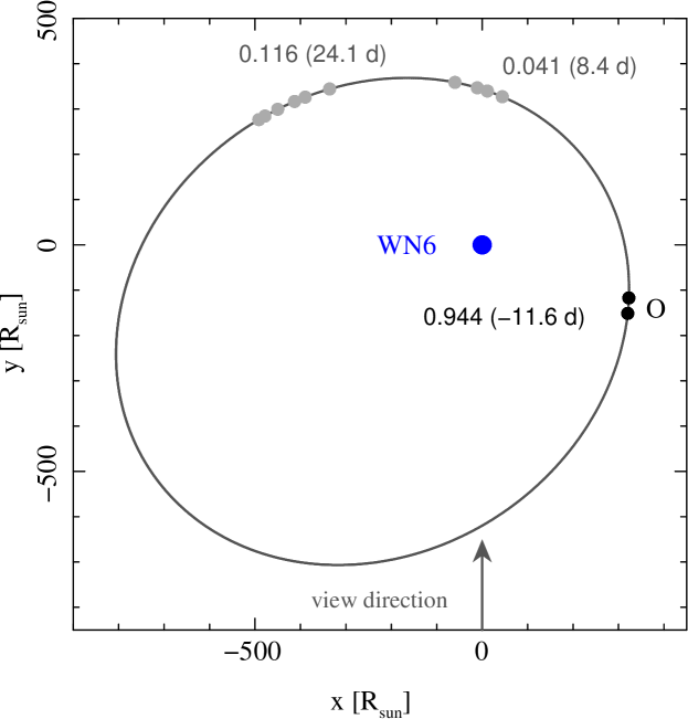
Figure 1: Schematic of the orbit of WR 25, viewed from above the orbital plane, referenced to the position of the WR-star primary, shown as the blue circle. Relative positions of the O-star secondary are shown as small circles for the on-axis HETG observations in black, and for the serendipitous off-axis observations in gray. Phases for the start of each group of observations are shown near the O-star circles, with days from periastron in parentheses.

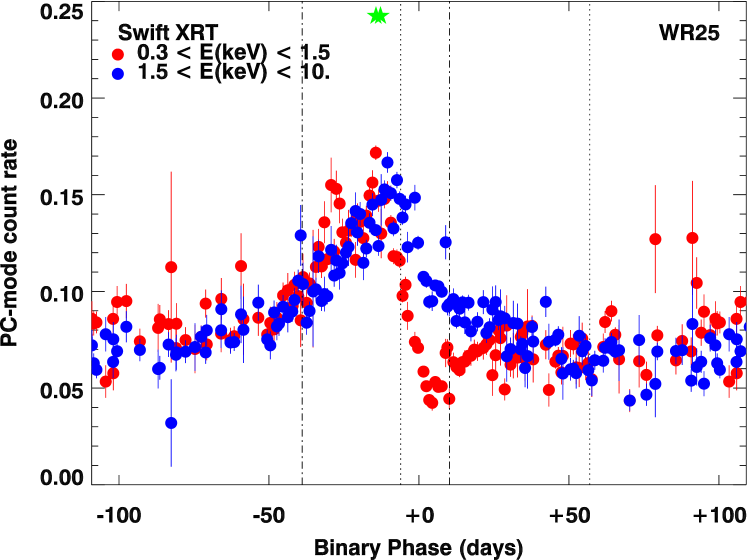
Figure 2: The Swift XRT light curve of WR 25 in two bands. The soft band ($0.3$–$1.5\,\mathrm{keV}$) is shown in red, and the hard band ($1.5$–$10\,\mathrm{keV}$) in blue. From the optical radial-velocity orbital solution, the vertical dotted lines mark quadratures (extrema in radial velocity), while the dot-dash vertical lines denote conjunctions, with the O-star in front about $40\,$days before periastron, and the WR-star in front at about $10\,$days after, where phase $0.0\,$days is periastron. Two overlapping green stars mark the phases of the pointed Chandra/HETGS observations at maximum light near quadrature corresponding to the black circles in Fig. 1.

From the mass-loss rates and terminal velocities in Table 1 the stagnation point of the colliding flows is expected to be closer to the O-star, and thus the shock cone convex towards the WR-star. Analysis by Arora et al. (2019) suggested that the wind velocity of each star at the stagnation point changes significantly over the course of the orbit, from about $1600\,\mathrm{km\,s^{-1}}$ at periastron to $2200\,\mathrm{km\,s^{-1}}$ at apastron, although this does not coincide with any obvious softening of the spectrum (Pollock & Corcoran, 2006). The shock may transition from adiabatic to radiative near periastron, and perhaps even undergo radiative braking (Gayley et al., 1997) through proximity to the intense O-star radiation field. The change in wind-wind collision pre-shock relative velocity from about $3200\,\mathrm{km\,s^{-1}}$ to $4400\,\mathrm{km\,s^{-1}}$ should result in a corresponding change in the post-shock temperature more than $50$%.

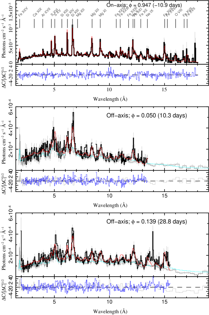
Figure 3: Top: Pointed Chandra/HETGS WR 25 flux spectrum (black), a powerlaw emission measure plasma model fit (red) and residuals (blue, lower panel). Center and bottom plots show the serendipitous off-axis HETGS spectra with their fitted high-resolution models convolved with a Gaussian appropriate for the off-axis blurring. The gray curve (with errorbars) is the zeroth order spectrum, and its corresponding model is the light solid line. The numbers in parentheses gives the days from periastron.

3 Observations

To better quantify the plasma conditions, we have obtained Chandra/HETG high-resolution X-ray spectra slightly before periastron (black circles in Figure 1, green stars in Figure 2), at phases in 2016 August when the Swift rates predicted a maximum. With these observations we can potentially determine line centroids, resolve lines widths, determine plasma temperatures from line strengths and the continuum shape, and constrain X-ray source locations from the photo-excitation in He-like ions’ forbidden-to-intercombination line ratios. From line-to-continuum ratios, we can explore possibilities of unusual abundances or collisionless plasma effects.

Although quite far off-axis ($\sim 10.5\,\mathrm{arcmin}$), we have also analyzed several serendipitous Chandra/HETG spectra of WR 25 taken more than 10 years earlier during high-resolution observations of other hot stars in Carina. The instrumental profile at the source locations is however too broad to characterize line widths or centroids accurately. The off-axis data provide some line and broad-band fluxes, useful for study of the stellar wind and wind-shock region structure through variations with phase.

Table 2 provides a log of the observations, exposure and the orbital phases, both for the on-axis and off-axis pointings.

Table 2: Table of observations analyzed in the current work with relevant time of observation, ObsID, exposure and orbital phases

Start Time	ObsID	Exposure	$\phi$	$\Delta\phi$
		[ks]		[days]
(on-axis pointings)
2016-08-10T15:19:33	https://heasarc.gsfc.nasa.gov/FTP/chandra/data/science/ao17/cat2//18616/ (catalog 18616)	28	0.944	-11.6
2016-08-11T23:28:52	https://heasarc.gsfc.nasa.gov/FTP/chandra/data/science/ao17/cat2//19687/ (catalog 19687)	57	0.951	-10.2
(serendipitous off-axis pointings)
2005-11-08T07:19:58	https://heasarc.gsfc.nasa.gov/FTP/chandra/data/science/ao06/cat2//7201/ (catalog 7201)	18	0.041	8.4
2005-11-09T14:44:53	https://heasarc.gsfc.nasa.gov/FTP/chandra/data/science/ao06/cat2//7204/ (catalog 7204)	33	0.047	9.7
2005-11-10T11:02:37	https://heasarc.gsfc.nasa.gov/FTP/chandra/data/science/ao06/cat2//7202/ (catalog 7202)	10	0.051	10.6
2005-11-12T07:41:15	https://heasarc.gsfc.nasa.gov/FTP/chandra/data/science/ao06/cat2//7203/ (catalog 7203)	27	0.060	12.4
2005-11-29T22:35:38	https://heasarc.gsfc.nasa.gov/FTP/chandra/data/science/ao06/cat2//5397/ (catalog 5397)	10	0.145	30.1
2005-12-01T12:19:53	https://heasarc.gsfc.nasa.gov/FTP/chandra/data/science/ao06/cat2//7228/ (catalog 7228)	20	0.152	31.6
2005-12-02T08:44:16	https://heasarc.gsfc.nasa.gov/FTP/chandra/data/science/ao06/cat2//7229/ (catalog 7229)	20	0.156	32.5
2006-06-19T18:00:43	https://heasarc.gsfc.nasa.gov/FTP/chandra/data/science/ao06/cat2//7341/ (catalog 7341)	53	0.116	24.1
2006-06-22T10:18:52	https://heasarc.gsfc.nasa.gov/FTP/chandra/data/science/ao06/cat2//7342/ (catalog 7342)	49	0.129	26.7
2006-06-23T17:45:18	https://heasarc.gsfc.nasa.gov/FTP/chandra/data/science/ao06/cat2//7189/ (catalog 7189)	18	0.135	28.0

4 High Resolution Spectral Analysis

4.1 On-axis observations

The counts spectra for the observations were extracted using TGCat reprocessing scripts (Huenemoerder et al., 2011), using CIAO (Fruscione et al., 2006) version 4.8 and Calibration Database version 4.7.2. Since the two on-axis observations are taken less than a day apart with orbital phases that differ by only $0.007$ (see Table 2), we combined the negative and positive first order spectra from both the observations to get one combined spectrum each for HEG and MEG. The advantage of doing this is to increase the signal-to-noise ratio facilitating high resolution spectral analysis, and also reducing the number of model bins, thereby reducing execution time in model evaluation during fitting.

We fit the spectra with both a global plasma model, and line-by-line. The global model gives a broad characterization of plasma conditions, within the parameters of the model, under the assumption that all the lines have the same shape and Doppler offset. The line-by-line fits relax the latter assumptions, and are independent of any global plasma model since they are local parametric functional fits.

For global spectral modeling, we fit the 1.5-20 $\text{\,}\mathrm{\SIUnitSymbolAngstrom}$ spectrum of WR 25 with a powerlaw emission measure distribution plasma model, as described in detail by Huenemoerder et al. (2020). The model is of the form, $dEM/dT=[n_{e}n_{H}\,dV/dT]\propto(T/T_{\mathrm{max}})^{-\beta}$, where $dEM/dT$ is the differential emission measure, $V$ is the volume of X-ray-emitting plasma, $n_{e}$ and $n_{H}$ are the electron and hydrogen number densities, respectively, $T$ is the plasma temperature which we limit to a range $T_{\mathrm{min}}$, $T_{\mathrm{max}}$, and the exponent on temperature is $\beta$. This model is obtained from line and continuum emissivites from the Astrophysical Plasma Emission Code (APEC) as stored in the atomic database, AtomDB (Smith et al., 2001; Foster et al., 2012). We used the abundances from Asplund et al. (2009). WR 25 likely has a reduced abundance of hydrogen and increased helium in the WN component. Hence interpretation of the normalization and relative abundances requires caution; Ignace et al. (2000) and Schulz et al. (2019) provide a method for scaling of parameters in low hydrogen plasmas. The model also assumes that all emission lines have the same Gaussian shape and Doppler shift, and that neutral absorption is all in the foreground. As such, the model represents the mean characteristics of the emitting plasma, and is not a detailed dynamical and geometrical model. Uncertainties on model parameters were determined from a Markov-Chain, Monte-Carlo evaluation. (an ISIS implementation, “emcee”, of the Foreman-Mackey et al., 2013, Python code) to search parameter space and form confidence contours.

The data, fitted model, and residuals are shown in the top panel of Fig. 3. The spectrum of WR 25 has many strong emission lines, primarily of H- and He-like ions, but also of many Fe ions. Below about $10\,\mathrm{{\mbox{\AA}}}$, the underlying continuum is also prominent. Model parameters are given in Table 3.

Table 3: Emission Measure Model Parameters

Parameter	Value	$\sigma$	Value	$\sigma$	Value	$\sigma$	Units
	$\phi=0.95$		$\phi=0.05$		$\phi=0.13$
$norm$	$0.032$	$0.003$	$0.025$	0.003	$0.024$	0.002	$\mathrm{cm^{-5}}$
$\beta$	$1.02$	$0.08$	$1.22$	0.09	$1.18$	0.07
$\log T_{\mathrm{max}}$	$7.70$	$0.03$	$7.93$	0.04	$7.82$	0.03	dex K
$\log T_{\mathrm{min}}$	$6.00$	(frozen)	–	–	–	–	dex K
$v_{\mathrm{turb}}$	$1338$	$42$	–	–	–	–	$\,\mathrm{km\,s^{-1}}$
$v_{\mathrm{Doppler}}$	$-303$	$32$	–	–	–	–	$\,\mathrm{km\,s^{-1}}$
$A(\mathrm{Ne})$	$0.60$	$0.09$	$0.48$	$0.11$	$0.42$	$0.05$
$A(\mathrm{Mg})$	$0.64$	$0.04$	$0.51$	$0.06$	$0.41$	$0.04$
$A(\mathrm{Si})$	$0.85$	$0.05$	$1.02$	$0.08$	$0.81$	$0.05$
$A(\mathrm{S})$	$1.10$	$0.10$	$1.73$	$0.20$	$1.20$	$0.10$
$A(\mathrm{Fe})$	$0.48$	$0.05$	$0.37$	$0.06$	$0.56$	$0.03$
$N_{\mathrm{H}}$	$0.65$	$0.04$	$0.74$	$0.05$	$0.56$	$0.03$	$10^{22}\,\mathrm{cm}^{-2}$
$f_{x}(obs)$	$1.01\text{\times}{10}^{-11}$		$6.14\text{\times}{10}^{-12}$		$6.11\text{\times}{10}^{-12}$		$\,\mathrm{ergs\,cm^{-2}\,s^{-1}}$
$f_{x}(N_{\mathrm{H}}=0)$	$3.70\text{\times}{10}^{-11}$		$2.98\text{\times}{10}^{-11}$		$2.71\text{\times}{10}^{-11}$		$\,\mathrm{ergs\,cm^{-2}\,s^{-1}}$

Note. — The normalization is related to the emission measure via $norm=[10^{-14}/(4\pi\,d^{2})]\int{n_{\mathrm{e}}n_{\mathrm{H}}\,dV}$, subject to re-interpretation for H-deficient, He-rich plasmas as stated in the text. The broadening was treated as a “turbulent” velocity term, added in quadrature to the thermal velocity and common to all ions. Abundances, $A(Z)$, are fractions by number relative to Asplund et al. (2009) (and were 1.0 if not listed). Uncertainties ($\sigma$) are given as a 68% confidence error-bars, as determined with Markov-Chain, Monte-Carlo methods. For the off-axis data ($\phi=0.05,\,0.13$), unspecified parameters were taken from the on-axis fits and frozen. Fluxes were evaluated from the fitted model over the band $1.0$–$40\,\mathrm{{\mbox{\AA}}}$ ($0.3$–$12\,\mathrm{keV}$). Pandey et al. (2014) estimated that the non-local ISM column to be about $0.37\times 10^{22}\,\mathrm{cm^{-2}}$.

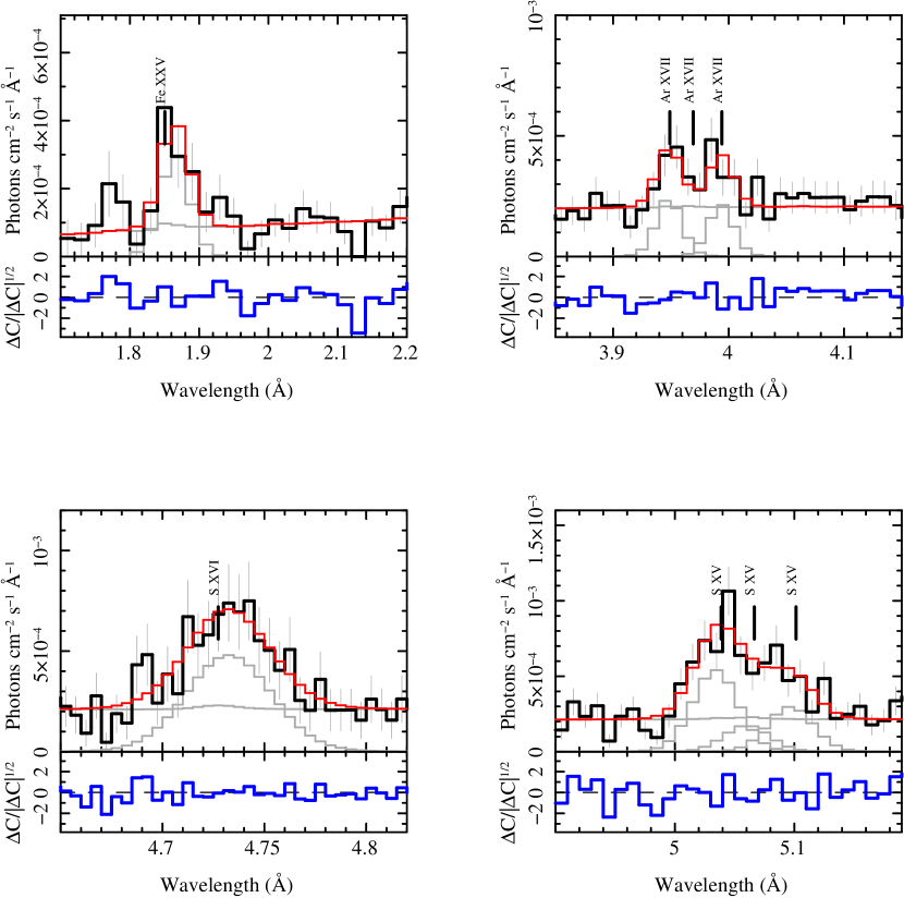
Figure A1: Gaussian fits to several emission line regions for the on-axis observations. In each panel, the black histogram shows the flux spectrum for the combined HETG first orders, the red is the model, the grey are the individual components of the model and the blue are the residuals.

Parametric line fitting was performed using the plasma model as a guide to line identification and probable blend assessment. Emission lines were fit in groups of overlapping or close features, using sums of Gaussian profiles folded through the instrument response. If features were too blended or too weak for unconstrained fits, they were restricted accordingly, either by constraining its parameters to a stronger line’s parameters (such as in using wavelength offsets or tied Gaussian $\sigma$), or by freezing the position or width and fitting the flux. The plasma model also served to provide a continuum model, since in crowded regions, with wind broadening, the local minima are not good approximations to the continuum. In these line fit models, we did not include neutral absorption, hence, the flux is as-observed at Earth. Emission line fit results are given in Table 4; for tied parameters in constrained fits, uncertainties have null values. The regions fit are shown in Figures A1, A2, A3.

We also examined the line profiles of strong lines in detail, considering whether a Gaussian shape is adequate, and we studied in detail the He-like ratios for evidence of photoexcitation in the forbidden-to-intercombination line ratio. Results will be discussed in subsequent sections.

Table 4: Emission Line Parameters for the on-axis observations.

Line	$\lambda_{0}$	$\Delta v$	$\sigma_{\Delta v}$	$f_{x}$	$\sigma_{f}$	$FWHM$	$\sigma_{FW}$
	Å	$\,\mathrm{km\,s^{-1}}$		$10^{-5}\,\mathrm{photons\,cm^{-2}\,s^{-1}}$		$\,\mathrm{km\,s^{-1}}$
Fe XXV	1.858	–	–	1.64	0.38	–	–
Ar XVII (r+i)	3.949	-56	238	0.69	0.18	1595	497
Ar XVII (f)	3.994	–	–	0.62	0.17	–	–
S XVI	4.730	162	215	2.55	0.35	2915	476
S XV (r)	5.039	-278	310	2.62	0.68	2453	446
S XV (i)	5.065	–	–	0.84	0.61	–	–
S XV (f)	5.102	–	–	1.44	0.34	–	–
Si XIII $\beta$	5.681	-266	326	1.18	0.28	2575	731
Si XIV	6.183	-263	65	4.83	0.26	2339	149
Si XIII (r)	6.648	-242	67	5.49	0.37	2303	135
Si XIII (i)	6.687	–	–	0.96	0.33	–	–
Si XIII (f)	6.740	–	–	2.97	0.23	–	–
Mg XII	8.422	-332	80	3.73	0.31	2160	198
Mg XI (r)	9.169	-291	133	3.20	0.37	1985	275
Mg XI (i)	9.230	–	–	0.57	0.36	–	–
Ne X	9.291	–	–	0.52	0.51	–	–
Mg XI (f)	9.314	–	–	0.47	0.52	–	–
Ne X	9.362	–	–	0.38	0.29	–	–
Ne X	9.481	–	–	0.20	0.21	–	–
Ne X	9.708	–	–	0.26	0.20	–	–
Ne X	12.135	-387	128	6.33	0.59	2568	292
Fe XVII	12.266	–	–	2.74	0.47	–	–
Fe XXI	12.390	–	–	2.78	0.48	–	–
Ne IX (r)	13.447	-526	147	2.99	0.68	1695	246
Fe XIX	13.497	–	–	0.11	0.48	–	–
Ne IX (i)	13.552	–	–	2.77	0.70	–	–
Ne IX (f)	13.699	–	–	1.69	0.51	–	–
Fe XVII	13.825	–	–	0.94	0.45	–	–
Fe XVII	15.014	-477	183	5.77	1.10	2466	498
Fe XVII	15.261	–	–	1.02	0.52	–	–
O VIII	16.006	-561	184	3.56	1.24	3441	1781
Fe XVII	17.051	–	–	2.04	1.14	–	–
Fe XVII	17.096	–	–	1.24	0.87	–	–

Note. — $\lambda_{0}$ is the theoretical wavelength and for each line, the velocity, error on velocity, flux, error on flux and full-width half maximum ($FWHM$), error on $FWHM$ are denoted by $\Delta v$, $\sigma_{\Delta v}$, $f_{x}$, $\sigma_{f}$, $FWHM$ and $\sigma_{FW}$ respectively. Only fluxes are reported for the lines where Gaussian width was frozen and where the wavelength was tied to their relative offsets from the resonance line. All errors are calculated for $1$-$\sigma$ confidence level limits.

4.2 Serendipitous Off-axis Observations

We analyzed 10 off-axis serendipitous observations of WR 25 (gray circles in Fig. 1 at phases $\sim 0.05$ and $\sim 0.14$). These were taken with the source at about $10\,\mathrm{arcmin}$ off-axis which significantly blurs the spectrum due to the large point-spread-function. The spatially broad spectra (in the cross-dispersion direction) were also truncated obliquely in some orders by the detector boundary, making the calibration uncertain. Hence we ignored wavelengths beyond about $14\,\mathrm{{\mbox{\AA}}}$. The shortest wavelengths, below about $2\,\mathrm{{\mbox{\AA}}}$, were also compromised by overlap of the wide HEG and MEG spectral arms, precluding extraction of Fe xxv.

To fit the HEG/MEG spectra, we determined the blur scale from the zeroth order extent, then used a Gaussian convolution model (Xspec’s “gsmooth”) on our APEC-based powerlaw emission measure model. Since the wavelength range of the dispersed off-axis spectrum is somewhat limited, we also simultaneously fit the zeroth-order spectra. Given the off-axis blurring of the image, CCD pile-up was not an issue, as it is for the on-axis zeroth order. To account for possible systematic differences in the zeroth order and dispersed effective area calibrations, we introduced an arbitrary renormalization factor on the zeroth order, whose value was $0.80\pm 0.01$, which is somewhat larger than the nominal $5\%$ expected calibration uncertainty. We fit this model to spectra in two phase groups (freezing the broadening and Doppler shift to the high-resolution fit values). Uncertainties were determined via emcee. The results are shown in Figure 3 and fitted parameters are listed in Table 3.

For the zeroth order spectra, we performed analysis only for the off-axis observations, since the on-axis spectra were heavily piled-up. We downloaded the relevant ObsIDs from TGCat (Huenemoerder et al., 2011) and used dmextract to extract the source spectrum by selecting circular regions of 60 arc-seconds centered on the source position. The relevant response files and the ancillary files were generated with mkacisrmf and mkarf. We corrected the ancillary files for the aperture efficiency factor using arfcorr as recommended in the CIAO website.

All spectral fitting was performed using the Interactive Spectral Interpretation System (ISIS software, Houck & Denicola, 2000), which also provides interfaces to AtomDB as well as to xspec (Arnaud, 1996) models.

5 Discussion

In a colliding-wind binary, the shocked-wind region far outshines the X-ray emission from the components’ stellar winds in isolation. The components of the WR 25 system are similar to $\zeta\,$Pup and WR 6, which have luminosities of about $6\times 10^{29}\,\mathrm{ergs\,s^{-1}}$ and $8\times 10^{32}\,\mathrm{ergs\,s^{-1}}$, respectively. If we assume the interstellar line-of-sight column density to WR 25 of $3.7\times 10^{21}\,\mathrm{cm^{-2}}$ estimated by Pandey et al. (2014), then the luminosity implied by the spectrum at $\phi=0.96$ is about $9\times 10^{33}\,\mathrm{ergs\,s^{-1}}$, nearly an order of magnitude larger than that expected from the individual stellar winds in isolation. The changing distance between the components around an eccentric orbit causes the wind-wind collision to occur at different velocities in the accelerating matter, and the varying aspect lets us view the shock from different angles, as well as through different wind columns of the two stars. Using high-resolution spectroscopy, we can therefore study the temperature and dynamics of the shock through line fluxes and profiles. The broad-band spectral shape is also sensitive to temperature and the line-of-sight neutral absorption.

Ideally, we would like to monitor the emission lines around the orbit. Hence, given only high-resolution spectra at just before periastron, this study represents only a start at a detailed view of WR 25 in high-resolution X-rays.

From the local line fits to the on-axis observations near $\phi=0.94$ (see Table 4 and Figures A1, A2, and A3), we find that there is a general blueshift of the centroid from the rest wavelength by about $-300\,\mathrm{km\,s^{-1}}$, with a possible decreasing trend in centriod with increasing wavelength. In Figure 4, the points with errorbars show these line-fit results. We also explored another approach, using the global plasma model as a starting point, and re-fit only the normalization, Doppler shift, and broadening in several wavelength regions. The global model, in contrast, used a common offset and broadening for all lines. This is of course not independent from the Gaussian line fitting, but takes advantage of the multiplexing of many features in the region, and using the underlying plasma model implicitly handles line blends. The result is shown as the shaded regions in Figure 4, and the trend with wavelength is very clear.

Since we are viewing the wind-wind collision shock-cone nearly edge on (perpendicularly to the line between stellar centers), we should expect broad lines with an apparent blue-shift if the receding material is obscured by foreground absorption by the shock-cone flow or stellar wind neutral plasma. In Figure 5, we can see that the lines are broad, and seem independent of wavelength.

The ratio of wind momenta, $\eta=(\dot{M}_{s}v_{\infty,s})/(\dot{M}_{p}v_{\infty,p})$, is in the range of $0.2$ to $0.5$, given the parameters in Arora et al. (2019). For these values, Pittard & Dawson (2018) find opening angles of the primary (WR-star) shock to be roughly $60^{\circ}$–$90^{\circ}$ (from the secondary to the stagnation point to the contact discontinuity line or primary shock envelope). At $\phi=0.94$ we should have a significant amount of plasma moving parallel to the line-of-sight (e.g., Henley et al., 2003), and indeed, we do see broad profiles, comparable to the primary’s wind velocity (Figure 5). Whether this is indeed due to the flow in the shock-cone will require spectra at phases near conjunctions, when such a flow would be transverse to the line-of-sight, and line widths would be smaller and have different velocity offsets.

Our plasma model assumes a power-law emission measure distribution. There is some theoretical justification for this form for stellar winds (Cassinelli et al., 2008; Krtička et al., 2009; Ignace et al., 2012). How well a power-law representation applies in colliding winds is an open question, though it does provide a reasonably good fit to the spectrum, as seen in Figure 3. The model has a parameter specifying a high-temperature cutoff. The continuum comes from thermal bremsstrahlung and bound-free processes, and each has an exponential cutoff at short wavelengths. Furthermore, the region below about $10\,\mathrm{{\mbox{\AA}}}$ has a strong continuum, relatively sparse emission lines from high-temperature ions, and is least affected by line-of-sight neutral plasma absorption. Hence, the high-temperature cutoff should be a fairly robust indicator of the maximum pre-shock velocities, under the assumption of strong shocks and collisional ionization equilibrium emissivities. Using the maximum temperature of $50\,\mathrm{MK}$ (see Table 3), a mean molecular weight, $\mu$ for a highly ionized plasma of $0.7$ appropriate for an He-enriched plasma (for comparison, abundances of Asplund et al. (2009) imply $\mu\sim 0.6$), and the relation for a strong shock, $kT=\frac{3}{16}\mu m_{\mathrm{H}}v^{2}$, in which $T$ is the post-shock temperature, $v$ is the pre-shock velocity, and $k$ is Boltzmann’s constant, we find a maximum relative shock velocity $v\approx 1918\,\mathrm{km\,s^{-1}}$ (with a formal statistical uncertainty of $66\,\mathrm{km\,s^{-1}}$). Arora et al. (2019) estimated that at $\phi=0.9$ each wind has a velocity of about $1800\,\mathrm{km\,s^{-1}}$ at the collision, so we might expect anything up to $3600\,\mathrm{km\,s^{-1}}$. Given that the emergent spectrum is from a larger region where plasma is cooling, our estimate is a plausible value.

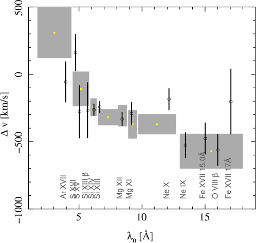
Figure 4: The line centroid velocity offsets from rest wavelengths is shown for two different approaches. The black circles with errorbars show the values from the Gaussian fits to line groups. The gray shaded rectangles show the result of piece-wise plasma model fits for the Doppler shift and broadening in several wavelength regions. Errorbars and gray shading vertical extent indicate one standard deviation uncertainties, while the gray rectangles’ widths indicate the wavelengthr region fit.

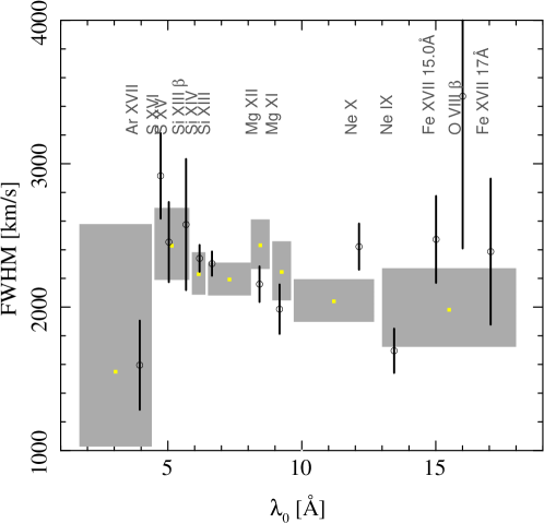
Figure 5: The line widths are shown from the Gaussian fits to line groups as points with errorbars, and from piece-wise plasma model fits, as in Figure 4.

5.1 Line Shapes

Our models, plasma or line-groups, have so far assumed Gaussian profiles. There is no a priori reason for the emission lines being Gaussian. The instrument response is highly Gaussian, but these are resolved features, with a $FWHM$ of several resolution elements. Henley et al. (2003) have shown how colliding wind regions could produce a wide variety of profiles, from narrow and single-peaked, to broad and double-peaked, suggesting a careful review of the observed line shapes.

The best, relatively isolated and strong feature in the WR 25 spectrum is that of the H-like Mg xii. This is an unresolved doublet with emissivities in a two-to-one ratio: $8.4192\,\mathrm{{\mbox{\AA}}}$ and $8.4246\,\mathrm{{\mbox{\AA}}}$, so the flux-weighted wavelength is $8.4210\,\mathrm{{\mbox{\AA}}}$. The only significant nearby feature, according to the plasma model, is Fe xxiii $8.3038\,\mathrm{{\mbox{\AA}}}$, with a flux at least 15 times smaller. To investigate whether lines are asymmetric, we fit the Mg xii region profiles with a Weibull distribution, whose shape can range from exponential, to Gaussian-like, to asymmetric with a tail on either the high or low side of the maximum:

$$f(\lambda;q,\sigma,\lambda_{0})=\frac{q}{\sigma}\,\left(\frac{\lambda-\lambda_{0}}{\sigma}\right)^{q-1}\,\exp\left[-\left(\frac{\lambda-\lambda_{0}}{\sigma}\right)^{q}\right]$$ (1)

in which $q>0$ is a shape parameter, $\sigma>0$ is a the scale, and $\lambda_{0}$ is an offset. We use the mode (maximum) as the line position:

$$\lambda_{\mathrm{max}}=\lambda_{0}+\sigma\left(\frac{q-1}{q}\right)^{\frac{1}{q}}$$ (2)

The model we fit was the sum of two Weibull functions (one for Mg xii and one for Fe xxiii) with common $q$ and $\sigma$ parameters, the wavelength offset and the relative strengths of the lines were constrained to their theoretical differences, plus a constant continuum, over the $8.0$–$9.0\,\mathrm{{\mbox{\AA}}}$ region. Given the best fit, we then determined confidence intervals via emcee, which also showed that $q$ and $\sigma$ were strongly correlated, with $q>4$ ($\sigma>0.1)$, but with values as large as $q=40$ preferred (and corresponding $\sigma=1.2$). The best fit has an asymmetric line, with a slightly more extended wing on the blue side. However, the acceptable value of $q=4$ is nearly Gaussian. The primary difference is that the peak is closer to the rest wavelength for the Weibull fit than for the Gaussian, which is probably offset to compensate for the slight asymmetry. Statistically, it is challenging to distinguish the difference, but the notion of some asymmetry agrees with expectations of more absorption at receding velocities. We show the fit and model profiles in Figure 6 and model parameters in Table 5.

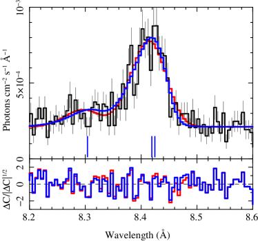
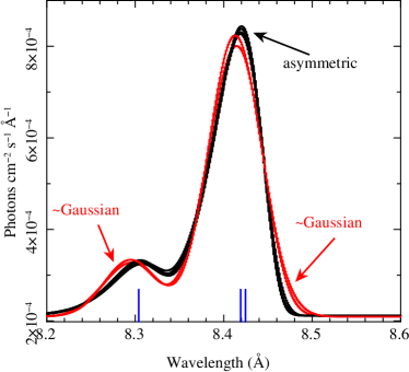
Figure 6: Left: The Mg xii region and fit with a Weibull distribution. The black histogram shows the data, the colored histograms show two models, and the lower panel the respective residuals. The strong feature is the Mg xii doublet at $8.42\,\mathrm{{\mbox{\AA}}}$; the weak feature at $8.3\,\mathrm{{\mbox{\AA}}}$ is an Fe xxiii line. The red model curve is for the $q=4$ (near Gaussian case), and blue is for $q=42$ (preferred solution). The blue residuals (lower panel) are slightly, but systematically, less than the red. Differences are very subtle, but slightly prefer the asymmetric model. Right: model profiles (unconvolved by the instrumental profile), all of them acceptable, for the $q=4$ (nearly Gaussian) and a Guassian fit (red curves, labeled “$\sim$Gaussian”), and for the slightly preferred Weibull fits with larger $q$ (black, labeled “asymmetric”). These serve as a key to the model curves in the left panel. The long vertical tic-marks on the $x$-axes in each plot mark the line rest wavelengths.

Table 5: Mg xii Region Weibull Fit Parameters

Parameter	Value	stddev	Units
$f($Mg xii$)$	$4.60$	$0.55$	$10^{-5}\,\mathrm{phot\,cm^{-2}\,s^{-1}}$
$\lambda_{\mathrm{max}}$	$8.4198$	$0.002$	Å
$\Delta v$	$-43.7$	$79.7$	$\,\mathrm{km\,s^{-1}}$
$\sigma$	$1.16$	$0.40$
$q$	$42.5$	$13.5$
$f($Fe xxiii$)$	$0.70$	$0.19$	$10^{-5}\,\mathrm{phot\,cm^{-2}\,s^{-1}}$
$f_{c}$	$20.03$	$0.55$	$10^{-5}\,\mathrm{phot\,cm^{-2}\,s^{-1}\,\,\mathrm{{\mbox{\AA}}}^{-1}}$

Note. — “stddev” is the one standard deviation uncertainty. The Fe xxiii line shared the parameters $\sigma$ and $q$, and was at a fixed wavelength offset from Mg xii of $-0.1181\,\mathrm{{\mbox{\AA}}}$.

An alternative approach has also clearly suggested asymmetry of the line profile. Following Pollock (2007), the HETG spectra at maximum light were fitted with an ensemble of lines with a single triangular velocity profile above an absorbed Bremsstrahlung continuum. A comparison was made between symmetric and asymmetric models, the latter parameterized by blue, central and red velocities showing where the profile reaches zero on either side of a central peak. The asymmetric model resulted in a C-Statistic improvement of ${\Delta}C=55.7$ for the single extra degree of freedom over the constrained symmetric model, clear evidence of a departure from symmetry with best-fit velocities having the blue intercept of $-2426\pm 103\,\mathrm{km\,s^{-1}}$, the peak occurring at $+61\pm 85\,\mathrm{km\,s^{-1}}$, and a red intercept of $+1525\pm 80\,\mathrm{km\,s^{-1}}.$

5.2 He-like Line Ratios

The He-like atomic structure has metastable levels which produce resonance ($r$), intercombination ($i$), and forbidden ($f$) lines in the soft X-ray band for several abundant elements, making them excellent diagnostics for temperature, density, and UV photoexcitation (Gabriel & Jordan, 1969; Blumenthal et al., 1972). These have been used to estimate the radius of formation of X-rays in OB-star winds (Waldron & Cassinelli, 2001; Leutenegger et al., 2006; Waldron & Cassinelli, 2007). An intense UV field can depopulate the forbidden line level, since they are metastable, and the closer the emitting plasma is to the UV-strong photosphere, the smaller the $f/i$ flux ratio. High density in plasmas can produce the same effect (Oskinova et al., 2017, c.f., ).

Since the X-ray flux of WR 25 comes predominantly from the shock cone, relatively far from the WR and OB star, we might not expect the $f/i$ ratio for Ne, Mg, and Si (for which we have good resolution) to be affected, unless there is a significant diffuse UV field produced in the shocks themselves. We have used our plasma model as a baseline for investigating the $f/i$ ratios in Ne ix, Mg xii, and Si xiii. Starting with this model, we introduce modified emissivities for the He-like lines using data produced from APEC (Foster et al., 2012). To let the model adjust locally to each He-like region investigated, we allowed the normalization, Doppler shift, line widths, and elemental abundances to be free, as well as the $f/i$ ratio parameter (we used density as a simple parameter to scale the ratio).

It is common to refer the ratio of the forbidden line flux to the intercombination line flux as, $R=f/i$. The expected value without UV or collisional pumping is usually denoted as $R_{0}$. This quantity has a mild temperature dependence, with about a $10\%$ increase with temperature where the line has significant emissivity. For $R_{0}$, we adopted the mean values as weighted by emission measure according to our adopted emission measure distribution model (see Section 4.1 and Table 3).

For Mg xi, we found that $R/R_{0}$ $>0.3$ (90% confidence) or $>0.4$ (68% confidence). Ne ix, at the 90% confidence level, spans the entire range; at 68%, it has $R/R_{0}>0.25$. The best fit for Si xiii is consistent with the unexcited limit; the 90% and 68% lower limits to $R/R_{0}$, respectively, are $0.65$ and $0.76$. Upper limits for Ne, Mg, and Si were all $1.0$, or in other words, they are consistent with no photo-excitation.

5.3 Variability

The Swift/XRT light curve indicates that the peak emission occurs around 10 days before periastron. The 0.3-1.5 keV XRT lightcurves exhibit a steep drop in the X-rays indicating increased absorption causing extinction of soft X-rays just after this peak and continues up to 10 days after periastron (Fig. 2).

The on-axis HETG observations were carried out just around maximum light as seen in the schematic diagram of the WR 25 orbit in Fig. 1. The times of these two observations are also indicated by green stars in Fig. 2.

The off-axis HETG spectra, while they are of too low a resolution for line shape or width determinations, do provide some spectral information. Further, the line fluxes and overall energy distribution provide some diagnostics of the plasma. We fit these spectra with the same absorbed powerlaw emission measure model as used for the on-axis spectra, and also assessed parameter confidence with emcee; model parameters are given in Table 3, and the spectra are shown in Figure 3. By $\phi=0.05$, the observed (absorbed) flux has dropped by about 40%, while the maximum temperature has risen from $50\,\mathrm{MK}$ to $85\,\mathrm{MK}$. The absorbing column has also risen; our sightline passes through more of the WR-star’s wind. The temperature increase is unexpected, since the stellar separations are about the same at the two phases, hence the wind-wind collision should be at the same relative velocity. At $\phi=0.13$, the absorption has dropped substantially as expected; the observed flux is about the same as at phase $0.05$. Here, we might expect the somewhat higher temperature as seen, given that the winds are expected to collide at a somewhat higher relative velocity. At the higher maximum plasma temperature, we estimate a shock relative velocity of $\sim 2200\,\mathrm{km\,s^{-1}}$.

The unabsorbed fluxes decrease steadily over the phase range from $0.95$ to $0.13$. We expect flux to generally scale inversely with the separation of the stars. Since it does not strictly do this, it may indicate other than adiabatic processes, as suggested by Arora et al. (2019), who estimated that radiative processes become important near periastron.

Within the pointed observation, there was significant short-term variability. In Figure 7 (left), we show the light curve of dispersed X-ray photons. There is significant variability, but it is not a constant rise with phase as the system approaches periastron. This could represent non-uniform density structure in the wind.

During the two on-axis observations, obsids 18616 and 19687, WR 25 was monitored optically with the Aspect Camera onboard Chandra. The Aspect Camera is mounted parallel to the X-ray telescope boresight and read continuously during the observation approximately every 2.05 s. The Aspect Camera CCD has a spectral response from 4000-10000 Å  so it is a redder wavelength range than Johnson UBV photometry. Flux calibration is based on a zero magnitude star of G0 V spectral type. Conversion between V and B magnitudes and Aspect Camera magnitudes is available in Nichols et al. (2010). It has been shown that the Aspect Camera photometry is internally consistent to 1-2%.

During the two on-axis observations, obsids 18616 and 19687, WR25 was monitored optically with the Aspect Camera onboard Chandra. The Aspect Camera is mounted parallel to the X-ray telescope boresight and read during the observation approximately every 2.05 s. The Aspect Camera CCD has a spectral response from 4000-10000 Å  so it is a redder wavelength range than Johnson UBV photometry. Flux calibration is based on a zero magnitude star of G0 V spectral type. Conversion between V and B magnitudes and Aspect Camera magnitudes is available in Nichols (2010). It has been shown that the Aspect Camera photometry is internally consistent to 1-2%.

Figure 7 (right) shows the Aspect Camera (ACA) data for ObsIDs https://heasarc.gsfc.nasa.gov/FTP/chandra/data/science/ao17/cat2//18616/ (catalog 18616) and https://heasarc.gsfc.nasa.gov/FTP/chandra/data/science/ao17/cat2//19687/ (catalog 19687) plotted with WR 25 phase and the ACA magnitude. It is surprising to find both light curves show a similar rise in brightness (lower magnitude). We verified that no high background event took place during the acquisition of these data, and all guide stars were well tracked during the entire observation (E. Martin, private communication). To estimate the error in ACA magnitude, we used the mean of the standard deviations of the ACA magnitudes for two of the guide stars used in this observation, deriving a value of 0.004 ACA magnitude. The two guide stars selected were clearly contant in ACA magnitude, so the errors we show for the ACA magnitude of WR 25 are assumed to be the errors associated with a constant source. The ACA data are broadband, with no spectral distribution information, so we cannot determine the cause of the change in magnitude during each observation. One possibility is a change in reddening, perhaps due to clumps of dust or density-enhanced gas clouds in the line of sight. WR 25 in fact lies in the line of sight to an enhanced thermal dust feature in Planck data. WR 25 has no intrinsic polarization (Fullard et al., 2020) but a large IPS angle (deviation of polarization angle with wavelength). Drissen et al. (1992) suggested that this deviation could be due to regions within the Carina Nebula that experience grain processing due to shock waves and the large IPS angle determined for WR 25 (Fullard et al., 2020) supports this idea. However, intrinsic dust in the WR 25 system could also produce a dust absorption signature. Optical and IR monitoring would be required to study the time-dependent absorption in this line-of-sight.

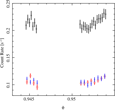
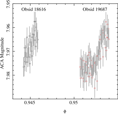
Figure 7: Left: We show the count-rate light curve for the on-axis pointings. The top shows the $1.7$ – $17.0\,\mathrm{{\mbox{\AA}}}$ band for HEG and MEG first orders. Below the curves are shown for two bands, subdivided at $7.25\,\mathrm{{\mbox{\AA}}}$; small (blue) circles are the short-wavelength range, and larger circles (red) the long-wavelength range. There is no appreciable change in the hardness ratio for these two bands. Error bars are one standard deviation, and time bins were about 1 hour. The $x$-axis range spans about $2.5\,$days at about $10\,$days before periastron. Right: The ACA magnitudes and estimated errors (see text) of WR 25 for ObsIDs https://heasarc.gsfc.nasa.gov/FTP/chandra/data/science/ao17/cat2//18616/ (catalog 18616) and https://heasarc.gsfc.nasa.gov/FTP/chandra/data/science/ao17/cat2//19687/ (catalog 19687). WR 25 was monitored with the optical ACA during these observations. The data are binned at 1 ks. The phase of the observations is shown on the X axis.

6 Conclusions

We have presented the first high-resolution X-ray spectra of the colliding wind binary WR 25, along with the context of long-term broad-band X-ray monitoring with Swift. The pointed HETGS observations were near periastron, when the X-ray brightness is maximal. The colliding wind shock region dominates the emission, being about an order of magnitude above that from similar spectral type stars which lack wind-wind collisions.

Our primary results from fitting the high-resolution lines and the energy distribution, under the assumption that the emitting plasma is in collisional ionization equilibrium, are:

1. The pre-shock velocity is about $v\approx 1918\,\mathrm{km\,s^{-1}}$;

2. Emission lines have a blue-shifted centroid which increases in magnitude with increasing wavelength, from about $-100\,\mathrm{km\,s^{-1}}$ to about $-600\,\mathrm{km\,s^{-1}}$. This is understood as likely due to the increased opacity of neutral matter which increasingly absorbs emission from receding plasma.

3. Emission lines are resolved and broad, with a $FWHM$ of about $2400\,\mathrm{km\,s^{-1}}$, with no clear trend with wavelength. This is consistent with the velocities of the colliding stellar winds seen nearly along the line-of-sight in a shock-cone. The constancy of the width with wavelength is somewhat at odds with the previous item, since increasing opacity with wavelength would hide receding material and narrow the lines. There might be significant turbulence in the shock-cone which masks bulk flow effects.

4. The emission lines seem very nearly Gaussian, though formally, a slightly asymmetric profile is preferred. The line shape depends critically on velocity fields and opacity. Hence, this should provide an important constraint for any detailed hydrodynamical models.

5. Within the HETGS observation, the source X-ray flux was significantly variable, at a level of about $15\%$. While phase coverage was small, the changes seemed gray and non-secular with phase. They may represent clumpiness in the wind and not, for instance, changing absorption or temperature.

The off-axis HETGS spectra, while higher resolution than imaging-mode, are blurred enough that line centroid and profile information are not available. The behavior does not show simple dependence on stellar separation, or phase, and may indicate that there non-adiabatic processes are significant near periastron. High resolution spectra are required at these phases in order to determine the dynamics, and to provide crucial constraints on wind-shock models. For instance, at $\phi\sim 0.04$ (conjunction), we expect the shock cone flow to be primarily away from us we would expect redshifted lines. The line width should also be smaller than near periastron since we are not viewing the cone transversely, but face on. At the other conjunction (O-star in front; $\phi\sim 0.8$, $-40\,$days), the shock cone would be concave toward the viewer, and we would expect blue-shifted lines.

WR 25 is perhaps the best system for studying colliding-wind physics. It is bright, has a period amenable to phase-resolved studies in a relatively short time span, and most importantly, it appears to stay relatively transparent to the O4-star even when looking through the WN 6 star’s wind. Other systems, such as WR 140 ($P\sim 8\,\mathrm{yrs}$) or $\eta\,$Car ($P\sim 5\,\mathrm{yrs}$) are quite opaque during conjunction and do not allow the shock-cone to be seen at soft X-ray energies. Blue-shifted lines have regularly been observed in colliding-wind binaries, notably in WR 140, but red-shifts only in $\theta\,$Muscae, a complex multiple system where orbital dynamics seem to play no role. In WR 140, absorption by the WC star wind at conjunction is far too strong for measurements to be feasible. The very massive WN systems Mk 34 and WR 21a both show deep extended minima at their relevant conjunction phases. While these are all interesting and relevant systems, WR 25 remains the best for studies of shock-cone dynamics about the whole orbit, and hence an excellent subject for study of stellar winds.

This study can only be considered as the initial investigation into the dynamics, since more phase coverage is needed. But we have shown that such a study is feasible and would likely be fruitful with the Chandra/HETGS.

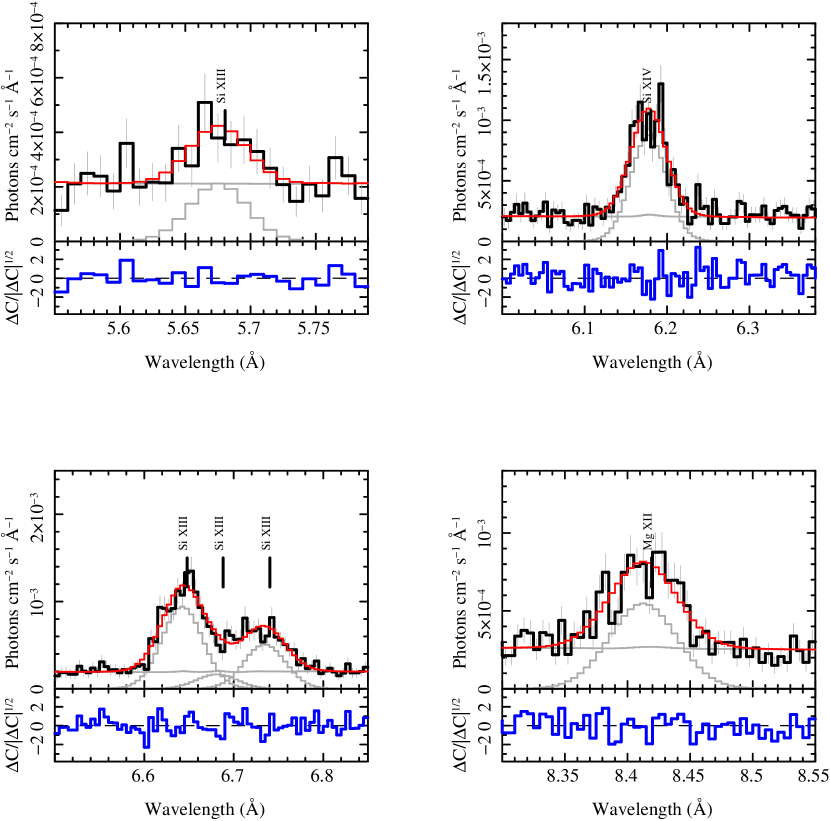
Figure A2: Gaussian fits to several emission line regions for the on-axis observations. In each panel, the black histogram shows the flux spectrum for the combined HETG first orders, the red is the model, the grey are the individual components of the model and the blue are the residuals.

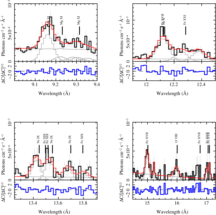
Figure A3: Gaussian fits to several emission line regions for the on-axis observations. In each panel, the black histogram shows the flux spectrum for the combined HETG first orders, the red is the model, the grey are the individual components of the model and the blue are the residuals.

References

- Arnaud (1996) Arnaud, K. A. 1996, in Astronomical Society of the Pacific Conference Series, Vol. 101, Astronomical Data Analysis Software and Systems V, ed. G. H. Jacoby & J. Barnes, 17–+
- Arora et al. (2019) Arora, B., Pandey, J. C., & De Becker, M. 2019, MNRAS, 487, 2624, doi: 10.1093/mnras/stz1447
- Asplund et al. (2009) Asplund, M., Grevesse, N., Sauval, A. J., & Scott, P. 2009, ARA&A, 47, 481, doi: 10.1146/annurev.astro.46.060407.145222
- Blumenthal et al. (1972) Blumenthal, G. R., Drake, G. W. F., & Tucker, W. H. 1972, ApJ, 172, 205, doi: 10.1086/151340
- Cantó et al. (1996) Cantó, J., Raga, A. C., & Wilkin, F. P. 1996, ApJ, 469, 729, doi: 10.1086/177820
- Cassinelli et al. (2008) Cassinelli, J. P., Ignace, R., Waldron, W. L., et al. 2008, ApJ, 683, 1052, doi: 10.1086/589760
- Castor et al. (1975) Castor, J. I., Abbott, D. C., & Klein, R. I. 1975, ApJ, 195, 157
- Corcoran et al. (2017) Corcoran, M. F., Liburd, J., Morris, D., et al. 2017, ApJ, 838, 45, doi: 10.3847/1538-4357/aa6347
- Crowther (2007) Crowther, P. A. 2007, ARA&A, 45, 177, doi: 10.1146/annurev.astro.45.051806.110615
- Crowther & Walborn (2011) Crowther, P. A., & Walborn, N. R. 2011, MNRAS, 416, 1311, doi: 10.1111/j.1365-2966.2011.19129.x
- Driessen et al. (2019) Driessen, F. A., Sundqvist, J. O., & Kee, N. D. 2019, A&A, 631, A172, doi: 10.1051/0004-6361/201936331
- Drissen et al. (1992) Drissen, L., Robert, C., & Moffat, A. F. J. 1992, ApJ, 386, 288, doi: 10.1086/171014
- Feldmeier et al. (1997) Feldmeier, A., Puls, J., & Pauldrach, A. W. A. 1997, A&A, 322, 878
- Foreman-Mackey et al. (2013) Foreman-Mackey, D., Hogg, D. W., Lang, D., & Goodman, J. 2013, PASP, 125, 306, doi: 10.1086/670067
- Foster et al. (2012) Foster, A. R., Ji, L., Smith, R. K., & Brickhouse, N. S. 2012, ApJ, 756, 128, doi: 10.1088/0004-637X/756/2/128
- Fruscione et al. (2006) Fruscione, A., McDowell, J. C., Allen, G. E., et al. 2006, in Presented at the Society of Photo-Optical Instrumentation Engineers (SPIE) Conference, Vol. 6270, SPIE Conference Series, doi: 10.1117/12.671760
- Fullard et al. (2020) Fullard, A. G., St-Louis, N., Moffat, A. F. J., et al. 2020, AJ, 159, 214, doi: 10.3847/1538-3881/ab8293
- Gabriel & Jordan (1969) Gabriel, A. H., & Jordan, C. 1969, MNRAS, 145, 241
- Gamen et al. (2006) Gamen, R., Gosset, E., Morrell, N., et al. 2006, A&A, 460, 777, doi: 10.1051/0004-6361:20065618
- Gamen et al. (2008) Gamen, R., Gosset, E., Morrell, N. I., et al. 2008, in Revista Mexicana de Astronomia y Astrofisica Conference Series, Vol. 33, Revista Mexicana de Astronomia y Astrofisica Conference Series, 91–93
- Gayley (2009) Gayley, K. G. 2009, ApJ, 703, 89, doi: 10.1088/0004-637X/703/1/89
- Gayley et al. (1997) Gayley, K. G., Owocki, S. P., & Cranmer, S. R. 1997, ApJ, 475, 786, doi: 10.1086/303573
- Grant et al. (2020) Grant, D., Blundell, K., & Matthews, J. 2020, MNRAS, 494, 17, doi: 10.1093/mnras/staa669
- Hamaguchi et al. (2016) Hamaguchi, K., Corcoran, M. F., Gull, T. R., et al. 2016, ApJ, 817, 23, doi: 10.3847/0004-637X/817/1/23
- Hamann et al. (2019) Hamann, W. R., Gräfener, G., Liermann, A., et al. 2019, A&A, 625, A57, doi: 10.1051/0004-6361/201834850
- Henley et al. (2003) Henley, D. B., Stevens, I. R., & Pittard, J. M. 2003, MNRAS, 346, 773, doi: 10.1111/j.1365-2966.2003.07121.x
- Houck & Denicola (2000) Houck, J. C., & Denicola, L. A. 2000, in Astronomical Society of the Pacific Conference Series, Vol. 216, Astronomical Data Analysis Software and Systems IX, ed. N. Manset, C. Veillet, & D. Crabtree, 591