Reconstructing teleparallel gravity with cosmic structure growth and expansion rate data
Abstract
In this work, we use a combined approach of Hubble parameter data together with redshift–space–distortion data, which together are used to reconstruct the teleparallel gravity (TG) Lagrangian via Gaussian processes (GP). The adopted Hubble data mainly comes from cosmic chronometers, while for the Type Ia supernovae data we use the latest jointly calibrated Pantheon compilation. Moreover, we consider two main GP covariance functions, namely the squared–exponential and Cauchy kernels in order to show consistency (to within 1 uncertainties). The core results of this work are the numerical reconstructions of the TG Lagrangian from GP reconstructed Hubble and growth data. We take different possible combinations of the datasets and kernels to illustrate any potential differences in this regard. We show that nontrivial cosmology beyond CDM falls within the uncertainties of the reconstructions from growth data, which therefore indicates no significant departure from the concordance cosmological model.
1 Introduction
The CDM cosmological model is overwhelmingly supported by a wide range of cosmological evidence at all cosmological scales [1, 2], which incorporates a significant portion of particle physics beyond the standard model [3]. In this setting, galactic structures are stabilised by cold dark matter [4, 5], and dark energy produces the observed late-time accelerated expansion [6, 7] through a cosmological constant [8, 9]. Despite decades of work, internal inconsistencies remain present in CDM cosmology [10, 11], while the possibility of direct measurements of dark matter continues to become more elusive [12].
Recent observations have called into question the predictive power of CDM cosmology, as its effectiveness in confronting cosmological tensions becomes an increasingly contentious issue [13]. Primarily, this has taken the form of differences in the values of the Hubble parameter with local, and cosmological model-independent, measurements from type Ia supernovae [14] and strong lensing by distant quasars [15] giving much higher values when compared with early Universe, and cosmology model-dependent, observations [16, 17]. While measurements from the tip of the red giant branch (TRGB, Carnegie-Chicago Hubble Program) and gravitational wave astronomy [18, 19, 20] point to a lower tension, a number of other works point to an even larger tension in the Hubble parameter [21, 22, 23]. A similarly important quantity that appears to be expressing a growing tension between local and early Universe measurements is that of the growth rate of large scale structures [16, 24]. In this context, the growth rate from a particular cosmological model (where is the linear matter overdensity), and the matter power spectrum normalised on scales of (see section 2) are combined in the parameter [25, 26] with being the cosmic scale factor. This parameter naturally emerges in cosmological theories of gravity through linear scalar perturbations and has been used in a number of analyses in competing theories of gravity beyond GR [2, 27].
Efforts continue to resolve these puzzling cosmological tensions within CDM through further analyses of the observations and considerations of more exotic particle physics beyond the standard model such as extended neutrino species. However, a full resolution may require the consideration of cosmological models beyond CDM [28, 29]. These are by and large described within the framework of curvature-based theories of gravity through the Levi-Civita connection [30]. More broadly, these theories of gravity can be classed as extensions to GR because they limit to an Einstein-Hilbert scenario in some parameter setting [29]. On the other hand, there is a growing body of work which considered gravity as an expression of torsion rather than curvature [31]. Torsion can be used to replace curvature in the geometric description of gravity by considering teleparallel gravity (TG) [32, 33] in which the teleparallel connection replaces the Levi-Civita connection.
TG represents a large class of theories in which the teleparallel connection is adopted [34] to describe gravitational interactions, which is torsion-full while being curvature-less and satisfying metricity. Thus, all curvature based measures identically vanish once this connection replaces the Levi-Civita connection. For instance, the Ricci scalar (over-circles denote all quantities that are calculated using the Levi-Civita connection) will vanish for the teleparallel connection, namely . Another important matter to point out is that a torsion scalar, , can be defined (see section 2) that is dynamically identical to the Einstein-Hilbert action in that it produces the same equations of motion. For this reason, a linear torsion scalar action generates the so-called teleparallel equivalent of general relativity (TEGR), which differs from GR by a boundary term in its Lagrangian density. The boundary, or total divergence, term in TEGR has a meaningful impact on possible extensions to TEGR and their relationship to extended gravity in GR [35, 36].
Using the same reasoning as in gravity [28, 29], TEGR can be arbitrarily generalised to gravity [32, 37, 38, 39, 40, 41, 42, 43]. This is a second-order theory that has shown in its confrontation with observations [32, 44, 45, 46, 47, 48, 49, 50, 51, 52, 53]. Also, gravity is fundamentally distinct from gravity in that to recover models in the latter case one must also include the boundary term (more details on this in Section 2.1) as in gravity [54, 55, 56, 57, 58, 59, 60, 61, 61, 62]. To fully recover an model, a specific subset of models must be selected, namely . gravity also has been tested against a number of observational phenomena with significant progress being made [63, 64, 60, 56, 59, 58, 61, 56, 65, 66, 67]. Another interesting extension to TEGR is gravity where is the teleparallel equivalent of the Gauss-Bonnet term [68, 69, 70, 71]. TG has also recently been used to construct a teleparallel analogue of Horndeski gravity [36, 72, 73] which is promising because it can bypass the problems related to the speed of gravitational waves in standard gravity. Observationally, gravity has shown promise in confronting cosmological data. In Refs. [44, 74, 52] it is shown that a number of viable models of gravity model cosmological data well for small deviations from CDM parameter values.
The problem with such larges classes of cosmological theories is that it is not intuitively clear which models have the potential to meet the observational challenges such as the recently reported cosmological tensions. Gaussian processes (GP) have an advantage in this regards in that they do not require one to have a specific parametrised cosmological model [75], and have been used in a number of diverse settings [76, 77, 78]. In terms of cosmological models in gravity, GP provides a model-independent approach that can lead to constraints on the form of the arbitrary Lagrangian that would normally require a specific model to be chosen.
In Ref. [79], this was first used to reconstruct the functional form using Hubble observational data. While in Ref. [80], the concept was expanded to include more data sets and prior values for the Hubble data. Also, this work provides a number of other GP reconstructed cosmological parameters such as the dark energy equation of state and the cosmological deceleration parameter. In the present work, this approach is extended into the perturbative regime through the parameter. In section 2 we give a brief review of gravity and its cosmology. While in section 3, we introduce the concepts behind GP reconstructions and apply them to both Hubble and redshift–space–distortion (RSD) data. Section 4 then contains the core results of this work in which we present constraints on the arbitrary function in cosmology. An interesting point of distinction between the present work and Ref. [80] is that in this other work an approximation had to be taken to produce initial conditions on the propagation equation for the Friedmann equation, whereas in the present study the growth equation does not require any restrictions to produce initial conditions. Finally, we summarise our results in section 5. Throughout the manuscript, Latin indices are used to refer to tangent space coordinates, while Greek indices refer to general manifold coordinates.
2 gravity
In this section, we show how gravity can be tested with observables related to its background and linear (scalar) perturbation equations. We connect the foundations of the theory with expansion and growth observables.
2.1 Cosmology
The curvature associated with GR is expressed through the Levi-Civita connection (over-circles are used throughout to denote quantities determined using the Levi-Civita connection) rather than the metric tensor which acts as the fundamental variable of the theory. The core distinction that TG represents is the exchange of the Levi-Civita connection with the teleparallel connection , which characterises gravitation through torsion while being curvature-less and satisfying metricity [81, 31]. The transition from the Levi-Civita to the teleparallel connection renders all curvature quantities such as the Riemann tensor organically zero (when calculated with the teleparallel connection). Thus, to construct theories of gravity in TG requires an entire new formulation of gravitational tensors (see reviews in Refs. [33, 32, 31]).
In TG, another important point to highlight is that the metric is no longer the fundamental dynamical object and is now derived from the tetrad (and its inverses ) through
| (2.1) |
where Latin indices represent coordinates on the tangent space while Greek indices represent coordinates on the general manifold. Tetrads also appear in GR but are reserved for specific usages [82]. These tetrads must also satisfy orthogonality conditions
| (2.2) |
for internal consistency. The teleparallel connection can then be defined as [34]
| (2.3) |
where is a flat spin connection that appears to incorporate the local Lorentz transformation (LLT) (namely Lorentz boosts and rotations) invariance of the theory [83]. In GR, spin connections are not flat and are largely hidden within the internal structure of the theory (and so do not contribute to the GR equations of motion) [84], whereas in TG they can have an important impact on the ensuing equations of motion (meaning that the spin connection explicitly appears in the generic field equations of the theory). For a particular choice of the Weitzenböck gauge, all of these components vanish [33]. In this context, a torsion tensor can be written as [32]
| (2.4) |
where square brackets denote an antisymmetric operator, and where this tensor represents the field strength of gravity in the TG framework [31]. The torsion tensor transforms covariantly under both diffeomorphisms and LLTs. By suitable contractions of the torsion tensor, the torsion scalar can be written through the representation [33, 32, 31]
| (2.5) |
which is entirely dependent on the teleparallel connection in the same way that the Ricci scalar depends only on the Levi-Civita connection.
For curvature-based gravity, the Levi-Civita connection produces the Ricci scalar which naturally vanishes when calculated using the curvature-less connection, meaning (where and ). By construction, the torsion scalar is built to be equivalent to the Ricci scalar up to a total divergence term , which can be represented as [56, 45]
| (2.6) |
This relation guarantees that the GR equations of motion are reproduced by an action based on a linear torsion scalar alone. Thus, making this the TEGR Lagrangian. Now, taking the same reasoning as in many extensions to GR, such as gravity [28, 29], the TEGR Lagrangian can be arbitrarily generalised to gravity through [37, 38, 39, 40, 41]
| (2.7) |
where , is the matter Lagrangian, and is the tetrad determinant. The core difference between and is that the total divergence term in Eq. (2.6) leads to fourth-order equations of motion in gravity, while gravity is generically second-order which is advantageous for numerous reasons, such as being organically Gauss-Ostrogadsky ghost free and being more amenable to numerical approaches. In Eq. (2.7), the functional form of appears as an extension to TEGR, meaning that CDM would correspond to a constant for the function in this setting. Finally, by performing variation of the action with respect to the tetrads, we arrive at the following field equations
| (2.8) |
where subscripts denote derivatives ( and ), and is the regular energy-momentum tensor.
In gravity, a flat homogeneous and isotropic Universe can be considered through the tetrad choice [83, 85]
| (2.9) |
where is the scale factor in cosmic time , and which reproduces the regular flat Friedmann–Lemaître–Robertson–Walker (FLRW) metric [84]
| (2.10) |
In this setting, and taking the Hubble parameter as where over-dots refer to derivatives with respect to cosmic time, we show all relevant cosmological scalar values in curvature and torsion based theories in Table. 1.
| Scalars | FLRW Value |
|---|---|
The tetrad corresponding to the FLRW metric can then be used to find the Friedmann equations as
| (2.11) | ||||
| (2.12) |
where we denote the energy density and pressure of the matter content by and , respectively.
2.2 Linear perturbations
Cosmological probes provide a number of measurements related to the evolution of cosmological perturbations. We will be using the growth rate measurements of from RSD, as described in section 3.2. By definition, the growth rate of cosmic structure , is given by the derivative of the logarithm of the matter perturbation with respect to the logarithm of the cosmic scale factor, namely
| (2.13) |
where a prime denotes a derivative with respect to redshift . Moreover, the linear theory root–mean–square mass fluctuation within a sphere of radius Mpc, where is the dimensionless Hubble constant, is given by
| (2.14) |
where a 0–subscript denotes the respective value at . Hence, the growth rate of structure can be written as follows,
| (2.15) |
Consequently, from the measurement, one can easily find the normalised evolution of via
| (2.16) |
By integrating Eq. (2.16), we can then determine the redshift evolution of the normalised matter density contrast
| (2.17) |
while from Eq. (2.16) we also get
| (2.18) |
From the above formalism, we can now determine the evolution of the derivative of with respect to , which is given by
| (2.19) |
In the subhorizon limit, the equation that governs the evolution of linear matter perturbations in the context of General Relativity and the majority of modified gravity models, is specified by
| (2.20) |
where is the effective Newton’s constant which is in general a function of and cosmic wavenumber . However, in this analysis will only be a function of redshift and –independent, since the adopted data is not sensitive to the –dependence [86, 87]. We now write Eq. (2.20) in terms of redshift, where we get
| (2.21) |
such that denotes the current matter fractional density, is Hubble’s constant, and is Newton’s gravitational constant. We can also express Eq. (2.21) in terms of the growth rate, which simplifies to the following
| (2.22) |
where we define the fractional change in the effective Gravitational coupling constant by
| (2.23) |
such that in General Relativity we have for any arbitrary redshift. In the case of gravity, the evolution equation (2.17) is satisfied with [88, 89, 52, 90]
| (2.24) |
Hence, from Eq. (2.24) one could infer the evolution of , which when combined with Eq. (2.11) we could then determine the functional form of via
| (2.25) |
3 Methodology
We devote this section to present and describe the adopted technique of GP, along with the data sets which will be used in the below analyses. We briefly mention the model dependencies and assumptions behind these data sets, which will therefore ensure the correct understanding to the range of validity of our results.
3.1 Gaussian processes
Similar to the definition of a multivariate normal distribution, which is specified by a vector of mean values and a covariance matrix, a Gaussian process [91, 75] is defined via a mean function , together with its associated two–point covariance function , such that we get a continuous realisation
| (3.1) |
and its corresponding uncertainty , leading to the realisation region of . The realisation region thus forms the posterior GP which is formed through a Bayesian iterative process in which a suitable covariance function is determined to model the datasets. Thus, for Gaussian distributed data the posterior distribution of the reconstructed function can be expressed via the joint Gaussian distribution of different data. A key element for this GP reconstruction is the kernel function which incorporates the uncertainties and correlations from observational data, along with the strength of the correlations between the reconstructed data points at distinct redshifts and (see Refs. [92, 93] for further details on its construction). There exists a number of kernel function templates [75, 92], and in this work we will be considering the customary infinitely differentiable squared–exponential kernel function
| (3.2) |
along with the Cauchy kernel function,
| (3.3) |
We consider two kernels to understand better any dependence on the choice of kernel function (we also define a Matérn kernel in appendix A which is used for comparison purposes) [94]. The so–called latent parameters or hyperparameters and , characterise the smoothness and overall profile of the GP reconstructed function [95], such that controls the uncertainties in the vertical direction as it compares the off–diagonal with the diagonal contributions, whereas adjusts the characteristic correlations’ length–scale in . Consequently, a large value of leads to a smoother GP function, whereas a higher value of is characterised by a lower signal–to–noise ratio. Hence, although the hyperparameters appear as constants, their values point to the behaviour of the underlying function, rather than a model that mimics this behaviour.
In order to find the properly suited values of the hyperparameters, we must make use of the observational data, which is itself a subset of realisations of the GP. Thus, the optimal values of the hyperparameters are derived from the maximisation of the probability of the GP to generate our considered set of data, that is implemented [96, 97, 92, 98] via the minimisation of the GP marginal likelihood, which is similar to the hierarchical Bayesian approach. GP have now been exhaustively used for the reconstruction of cosmological functions, particularly related to the late–time cosmic accelerated expansion observables [99, 92, 100, 101, 102, 103, 79, 104, 93, 105, 106, 107, 108, 109, 80, 110]. We should remark that although GP are independent from any cosmological model, GP rely on the choice of the kernel function which governs the correlations between distinct points in the GP reconstructed function, and hence its profile. This is particularly noticeable at those locations which lack observational data points. As discussed above, we therefore consider different kernel functions in order to address this kernel dependent characteristic.
3.2 Observational data sets
We here discuss the adopted cosmological data which incorporates probes of the expansion rate of the Universe, as well as the growth rate of cosmic structure. We also illustrate the respective direct GP reconstructions of and , which will be further exploited in section 4.
3.2.1 Hubble parameter data
We first focus on the Hubble parameter data points which we get from cosmic chronometers (CC), along with a Type Ia supernovae (SN) compilation data set. CC data allows us to obtain direct information about the Hubble function at several redshifts, up to around , contrary to other cosmological probes which have to derive the value of from other observables. Since this technique is primarily based on measurements of the age difference between two passively–evolving galaxies that formed at the same time but are separated by a small redshift interval (from which one can compute ), CC were found to be more reliable than any other method based on an absolute age determination for galaxies [111]. Our CC data points coincide with the considered data sets of Refs. [93, 109, 80], which were compiled from Refs. [112, 113, 114, 115, 116, 117, 118]. We should remark that these CC measurements are independent of the Cepheid distance scale and from any cosmological model, although they rely on the modelling of stellar ages, which depend on robust stellar population synthesis techniques (see, for instance, Refs. [93, 119, 120, 97, 116, 114] for analyses related to CC systematics).
For the SN data, we use a jointly calibrated and compressed data set [121] consisting of the Pantheon compilation [122], which includes SN at , along with another 15 SN at from the CANDELS and CLASH Multi–Cycle Treasury programs [121]. We use the reported Hubble rate parameter measurements of in the redshift range of , along with the corresponding correlation matrix, where only five of the reported six data points are adopted since the data point is not Gaussian–distributed (similar to Refs. [93, 80]). We should mention that the considered SN inferred measurements could not be considered as a model independent data set, since a spatially flat Universe was assumed in Ref. [121]. However, this reasonable assumption has a negligible impact on our analyses, as we are assuming a spatially flat Universe, and the best constraints on spatial curvature [17, 16] are in very good agreement with this assumption. Moreover, at these low redshifts, the deviation in due to a minute spatial curvature contribution is much less than the current uncertainties of the adopted SN data points. CC and SN data provides an interesting contrast since they originate from distinct physical processes. In the literature, CC data alone has not been enough to adequately constrain various models and so, we also include the SN data for comparative purposes.
In order to incorporate the SN data set in our GP analyses, we make use of an iterative numerical procedure [93, 80] to determine an value from GP. Basically, we first infer an value by applying GP to the CC data set only, and then we promote the SN data points to the corresponding values via a Monte Carlo routine. A number of successive GP reconstructions are applied on the combined CC + SN data set, until the resulting value of and its uncertainty converge to .
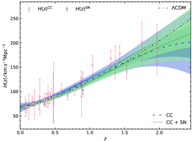
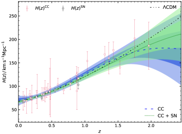
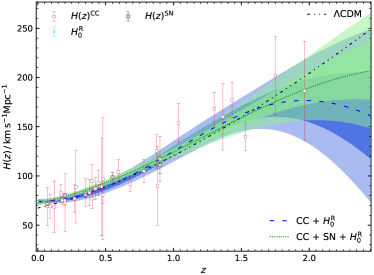
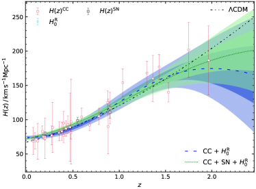
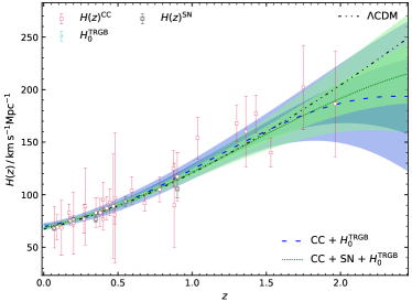
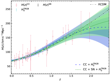
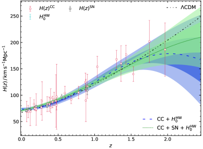
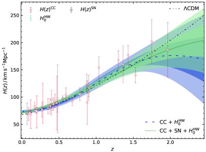
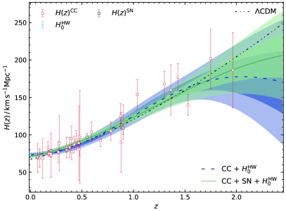
We further consider a number of recently reported local measurements of . We will be adopting the currently highest value of [14] determined via long period observations of Cepheids in the Large Magellanic Cloud, along with [123] which was based on the Tip of the Red Giant Branch (TRGB) as a standard candle. Another recent determination of was reported by the strong lensing H0LiCOW Collaboration [15], with . We illustrate the GP reconstructions of with the mentioned priors and different kernel functions in Fig. 1, while we depict similar results with the prior in appendix A.
While other measurements exist (for instance, as reported in Refs. [124, 16, 125]), the aforementioned measurements are the most representative model independent values. We should further remark that we decided to use the above mentioned values in light of the current –tension conundrum [13, 126, 127, 128, 129, 130], such that we can analyse the impact of a chosen prior on our GP reconstructions of section 4.
3.2.2 Growth rate data
We now consider the growth of cosmic structure measurements. It is well–known that maps of galaxies where distances are measured from spectroscopic redshifts are characterised by anisotropic deviations from the true galaxy distribution. Such differences arise due to the galaxy’s recessional velocities which include contributions from both the Hubble flow, and peculiar velocities from the motions of galaxies in comoving space. Although these RSD [131] can be considered as a nuisance when trying to reconstruct the true spatial distribution of galaxies, RSD unequivocally encode information on the evolution of cosmic structure formation. Since the evolution and formation of cosmic structure is implicitly governed by the underlying theory of gravitation, RSD offers another very promising avenue to test modified theories of gravity (see, for instance, Refs. [132, 133, 134, 135, 136, 25]).
Although the growth rate can be obtained from RSD cosmological probes and used to constrain cosmological models (see, for instance, Refs. [137, 138]), RSD measurements are very often reported in terms of the more reliable (since it evades the issue related to the bias parameter [25]) density–weighted growth rate . We should also remark that RSD measurements are also sensitive to [139]. The latter could be properly computed via the low–redshift RSD measurements, as it (nearly) evades the extrapolation from a fiducial cosmological model, an assumption which could not be avoided in the case of CMB data sets.
Furthermore, galaxy surveys often have to consider degeneracies between RSDs and the so–called Alcock–Paczynski effect [140], which arises from the need to assume a cosmological model to transform redshifts into distances. At low redshifts this effect is not significant, meaning that our considered measurements are fairly independent of the choice of the fiducial cosmological model. We have adopted the rough approximation [141, 25, 107] of the Alcock–Paczynski effect by re–scaling the growth rate measurements and uncertainties by the ratio of , where is the angular diameter distance, although it should be noted that our final results were not affected by this re-scaling.
| Kernel | |
|---|---|
| Squared–exponential | |
| Cauchy |
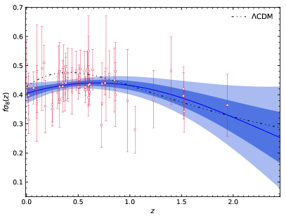
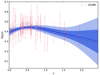
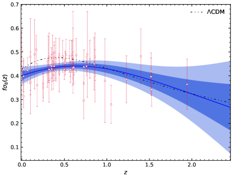
Our data set consists of all RSD measurements along with the respective covariance matrix as reported in Ref. [25]. This data set incorporates a number of large–scale structure surveys which were ongoing from 2006 to 2018 [142, 143, 144, 145, 146, 147, 148, 149, 150, 151, 152, 153, 154, 155, 156, 157, 158, 159, 160, 161, 162, 163, 164]. We illustrate the GP reconstructions of with the squared–exponential and Cauchy kernel functions in Fig. 2 (while in Fig. 9 we depict the reconstruction with the Matérn kernel function). As indicated in Table 2, the current GP reconstructed values of the density–weighted growth rates from the squared–exponential and Cauchy kernel functions are nearly identical. The reconstructions are nearly indistinguishable at low redshifts, although at higher redshifts, coinciding with the redshift range where there are less data points, the Cauchy (and Matérn) kernel function(s) tend to be characterised by a larger uncertainty with respect to the squared–exponential kernel function. It is also clear that the concordance model of cosmology agrees very well with the reconstructed , although for the CDM model with Planck’s baseline parameters [16] predicts a higher growth rate than the RSD’s GP reconstructed evolution.
We should mention that we had to modify the standard approach as described in section 3.1 for finding the optimal GP hyperparameters, since such a technique leads to an unrealistically flat GP reconstruction of . We derived the optimal values of the hyperparameters by sampling the logarithm of the GP marginal likelihood on a grid of hyperparameters and , from 0.01 to the maximum redshift of data points of , with equally spaced points in log–space for each dimension [165]. This now ensures that the typical scale , on the independent variable is always smaller than the redshift range of our data set. We then select the pair of hyperparameters corresponding to the maximum of the log–marginal likelihood, which turn out to be different from those derived via the standard GP approach, consequently improving the determination of this observable.
4 Results
In our analyses, we perform a number of GP reconstructions using a combination of two choices, the first being the prior which is selected from having no prior, or one of the or values (we consider the prior in appendix A), while the second involves the squared–exponential or Cauchy GP kernel functions (refer to appendix A for a comparative analysis with the Matérn kernel function). Our GP analyses were implemented in a modified version of the public code GaPP (Gaussian Processes in Python)222http://ascl.net/1303.027 [95], which was specifically developed for the GP reconstruction of a function and its derivatives from a given data set.
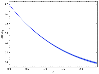
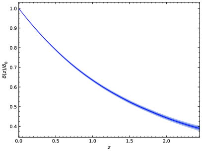
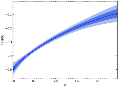
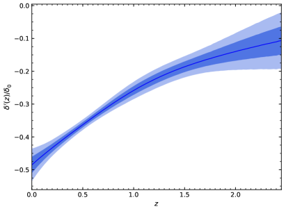
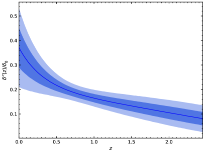
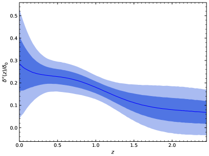
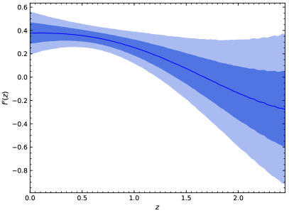
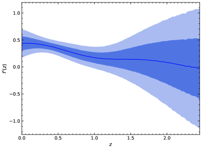
In order to reconstruct the function from the data sets of section 3.2, we need to reconstruct other functions describing the cosmological background evolution as well as the evolution of the matter density contrast. From the GP reconstructions of the considered data, which we illustrate in the panels of Fig. 2, we utilise Eqs. (2.16)–(2.18) to reconstruct the redshift evolution of the , and functions. We depict the GP reconstructions of the normalised density contrast and its first and second derivatives in Fig. 3, where we make use of the squared–exponential and Cauchy kernel functions. For these reconstructions, we have further adopted Planck’s baseline parameter value of [16]. From the top panels of Fig. 3, it is clear that there is an insignificant influence from the choice of kernel functions on the reconstruction of . However, this statement does not robustly hold for the reconstructions of the first and second derivative of the normalised matter density contrast. Indeed, the mean realisation and the corresponding confidence regions of differ between the GP reconstruction adopting the squared–exponential kernel function with respect to the GP reconstruction using the Cauchy kernel function. Such a difference is more prominent in the reconstruction of the second derivative of , where we could observe that in general the squared–exponential kernel function leads to a smoother and more uniform GP reconstruction relative to the one obtained via the Cauchy kernel function. Moreover, the GP reconstructions of and with the Cauchy kernel function are characterised by a more conservative confidence region than the respective GP reconstructions with the squared–exponential kernel function.
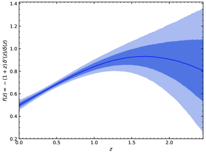
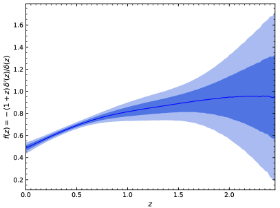
We can now map the obtained GP reconstructions of the matter density contrast and its derivatives, to the GP reconstruction of the matter growth rate function with the use of Eq. (2.13). Furthermore, we can also infer the evolution of from Eq. (2.19), which utilises all the previously reconstructed functions of the normalised matter density contrast. The redshift evolution of the reconstructed functions of and are respectively depicted in the top and bottom panels of Fig. 4. Further to the above discussion, the squared–exponential kernel function led to more uniform and slightly tighter GP reconstructions with respect to those inferred via the Cauchy kernel function, although the computed GP reconstructions from the two kernel functions are consistent with one another.
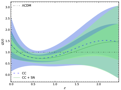
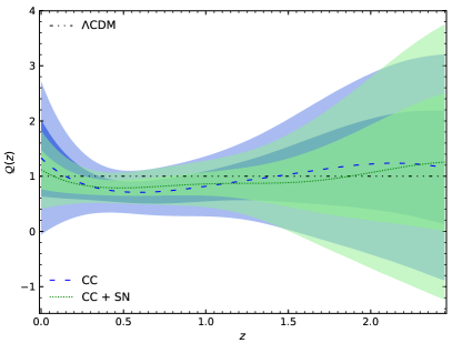
We are now in a position to reconstruct the fractional change in the effective Gravitational coupling function via Eq. (2.24), where we have further assumed that [16]. For the GP reconstruction of we also have to adopt a value of Hubble’s constant, which we infer from the GP reconstruction of , and when applicable, an prior will also be considered. Since we focus on the reconstruction of without a local prior, and the reconstruction of in the presence of the and priors, we will have three scenarios for each choice of kernel functions, as depicted in the left–hand and right–hand panels of Fig. 5.
One could clearly notice that in the case of CC and CC + SN data sets without a local prior, the squared–exponential and Cauchy kernel functions led to , which is in full agreement with the elementary concordance model of cosmology. However, in the presence of an prior, particularly , the GP reconstructed function of is more dynamical and in the range of we find that deviates from unity by . As expected, such deviation is suppressed when we use the Cauchy kernel function, since all previously inferred GP reconstructions with this kernel function were always found to be more conservative than the corresponding results with the squared–exponential kernel function. Indeed, is always found to be in agreement with unity when we utilise the Cauchy kernel function in the presence or absence of the considered priors on the Hubble constant.
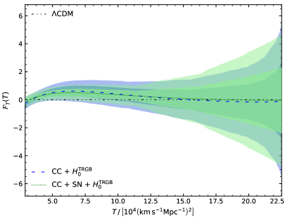
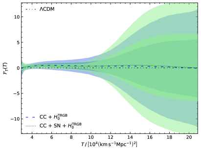
From the above reconstructions of , we can easily reconstruct the redshift evolution of via Eq. (2.24). We further express the GP reconstructed function of as a function of , by mapping the GP reconstructed to the torsion scalar via Table. 1. The evolution of the GP reconstructed functions are illustrated in the panels of Fig. 6, where the left–hand side and right–hand side panels correspond respectively to the reconstructions with the squared–exponential and Cauchy kernel functions. Further to the above discussion, the Cauchy kernel function was again characterised by more conservative constraints on with respect to those inferred with the squared–exponential kernel function. Moreover, it is clear that the joint CC + SN data set led to tighter constraints with respect to the CC data. All reconstructions of were found to be consistent with a null value; in full agreement with the CDM model. We should remark that even in the case of the prior, the confidence region of the GP reconstruction was always consistent with a null value.
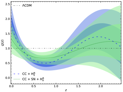
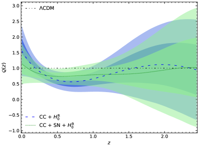
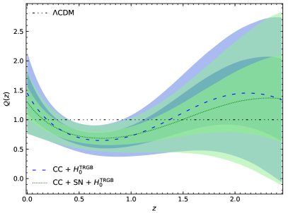
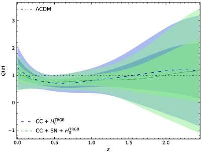
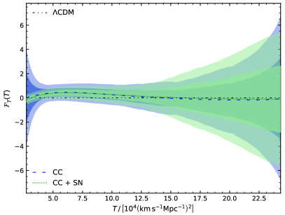
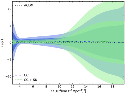
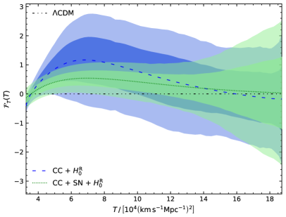
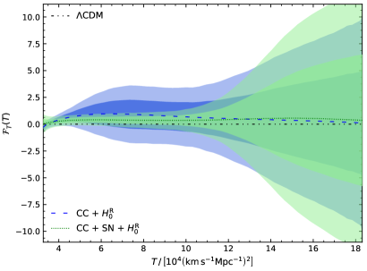
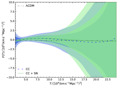
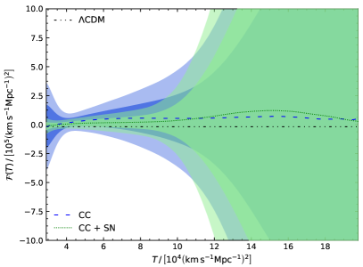
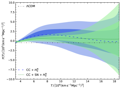
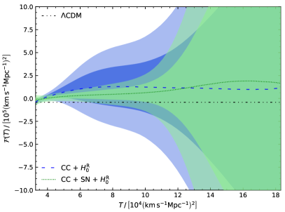
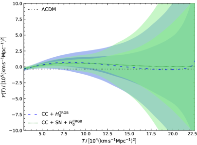
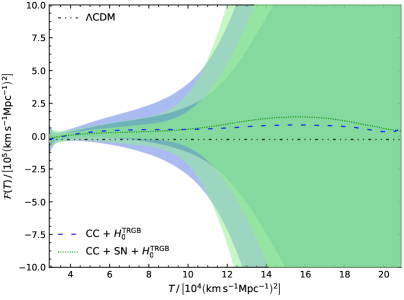
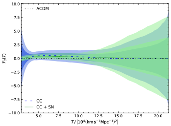
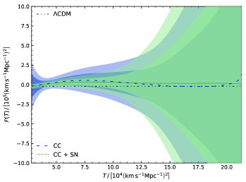
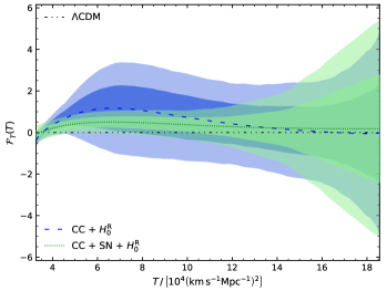
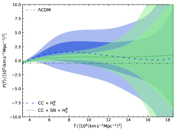
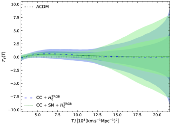
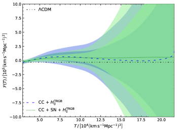
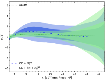
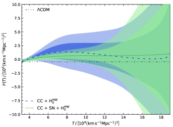
We finally reconstruct the function via Eq. (2.25) where we depict the GP reconstructions in Fig. 7. The GP reconstructions of were found to be weakly constrained at high values of (corresponding to high– values), particularly with the Cauchy kernel function. Furthermore, the GP reconstructions of are consistent with the CDM theoretical prediction, although at very low values of (low–), there is a slight departure from the corresponding CDM value when we adopt , and mildly with . Such a low–redshift deviation from the CDM model could be attributed to the disagreement between the high value and the preferred (GP reconstructed) value of with the CC and CC + SN data sets, leaving a small redshift window for a plausible and competitive model.
5 Conclusions
GP is a stochastic process that offers an interesting approach to modeling the behaviour of data. In the cosmological context, GP are an effective setting in which to investigate cosmological parameters such as the Hubble and parameters. These parameter values have led to intense debate in recent years with numerous approaches being explored [166]. In this work, we continue to build on recent works in which cosmological data is used to constrain the arbitrary Lagrangian within a broad cosmology beyond CDM, which in this instance is gravity. In Refs.[79, 80, 167], the idea of using Hubble data to reconstruct the Lagrangian was explored together with other background cosmological parameters such as the deceleration and equation of state parameters (which are consistent with the current work). In the present work, this approach was extended to growth rate data wherein this data was used to constrain the values of the Lagrangian. This is the first time (to the best of our knowledge) that growth rate data has been used in this way. Moreover, this provides a crucial consistency check on the results from the background analysis.
To achieve this, we use the Friedmann equation in Eq. (2.11) to reconstruct Hubble data, and in conjunction with the linear perturbation equation associated with scalar perturbations, we determine values of using Eq. (2.25). To test the model independence of the GP approach, we utilised two main kernel functions, namely the squared–exponential and Cauchy covariance functions, as well as the Matérn kernel in the appendix (for comparison purposes). To within 1 confidence level, the ensuing results are consistent with each other. In all cases, we consider the effects of CC and CC + SN datasets separately for these kernels, which are also considered in the context of and priors for the background setting. For the growth rate data we considered RSD data, which in combination, provides reliable restrictions on the possible values of the functional form of . However, for larger redshift values, these constraints are not very restrictive due to the lack of data points at these redshifts. Also, the combined data set errors has an effect on the reconstruction uncertainties.
These GP reconstructions are depicted in Fig. 7, where the Lagrangian functional form is shown against the torsion scalar argument. While are well constrained at low redshifts, the situation for higher redshifts becomes exceedingly unconstrained. This is most expressed for the prior settings due to the very large value of in this circumstance. On the other hand, the also points to an increase in the uncertainties at lower redshifts but the impact is not as strong as under the prior setting. We should finally remark that the inferred GP reconstructions of the Lagrangian would further instigate the ongoing development of the theoretical framework, and its confrontation with cosmological data sets.
Acknowledgments
The authors would like to acknowledge networking support by the COST Action CA18108 and funding support from Cosmology@MALTA which is supported by the University of Malta. This research has been carried out using computational facilities procured through the European Regional Development Fund, Project No. ERDF-080 “A supercomputing laboratory for the University of Malta”.
Appendix A Additional comparisons
We here illustrate the inferred GP reconstructions with the prior along with a comparative analysis of results obtained with the squared–exponential, Cauchy, and Matérn kernel functions, where the latter kernel function is given by
| (A.1) |
We illustrate the similarities between the GP reconstructions when utilising different kernel functions in Fig. 8, while in Fig. 9 we depict the GP reconstruction of with the Matérn kernel function. From the latter figures, it should be noted that there is a very good agreement with the corresponding GP reconstructions (see, Figs. 1–2) inferred with the squared–exponential kernel function. Indeed, the current GP reconstructed value of the density–weighted growth rate with the Matérn kernel function is of , which is nearly identical to the GP reconstructed values from the squared–exponential and Cauchy kernel functions as reported in section 3.2.2.
Since [15], lies between [14] and [123], it is expected that the GP reconstructions will be in agreement with the and GP reconstructions. Indeed, this is clearly depicted in the panels of Fig. 10. Moreover, since is closer to the mean value of than to , the resulting GP reconstructions are very similar to the GP reconstructions. Consequently, we do not discuss the GP reconstructions in the main text, but we illustrate such similarity in this appendix for completeness purposes.
References
- [1] S. Dodelson, Modern Cosmology. Academic Press, 2003.
- [2] T. Clifton, P. G. Ferreira, A. Padilla and C. Skordis, Modified Gravity and Cosmology, Phys. Rept. 513 (2012) 1 [1106.2476].
- [3] S. Weinberg, The Quantum Theory of Fields, vol. 1. Cambridge University Press, 1995, 10.1017/CBO9781139644167.
- [4] L. Baudis, Dark matter detection, J. Phys. G43 (2016) 044001.
- [5] G. Bertone, D. Hooper and J. Silk, Particle dark matter: Evidence, candidates and constraints, Phys. Rept. 405 (2005) 279 [hep-ph/0404175].
- [6] Supernova Search Team collaboration, Observational evidence from supernovae for an accelerating universe and a cosmological constant, Astron.J. 116 (1998) 1009 [astro-ph/9805201].
- [7] Supernova Cosmology Project collaboration, Measurements of and from 42 high redshift supernovae, Astrophys.J. 517 (1999) 565 [astro-ph/9812133].
- [8] P. J. E. Peebles and B. Ratra, The Cosmological constant and dark energy, Rev. Mod. Phys. 75 (2003) 559 [astro-ph/0207347].
- [9] E. J. Copeland, M. Sami and S. Tsujikawa, Dynamics of dark energy, Int. J. Mod. Phys. D 15 (2006) 1753 [hep-th/0603057].
- [10] R. J. Adler, B. Casey and O. C. Jacob, Vacuum catastrophe: An elementary exposition of the cosmological constant problem, Am. J. Phys. 63 (1995) 620.
- [11] S. Weinberg, The cosmological constant problem, Rev. Mod. Phys. 61 (1989) 1.
- [12] R. J. Gaitskell, Direct detection of dark matter, Ann. Rev. Nucl. Part. Sci. 54 (2004) 315.
- [13] E. Di Valentino et al., Cosmology Intertwined II: The Hubble Constant Tension, 2008.11284.
- [14] A. G. Riess, S. Casertano, W. Yuan, L. M. Macri and D. Scolnic, Large Magellanic Cloud Cepheid Standards provide a 1% foundation for the determination of the Hubble constant and stronger evidence for physics beyond CDM, Astrophys. J. 876 (2019) 85 [1903.07603].
- [15] K. C. Wong et al., H0LiCOW XIII. A 2.4% measurement of from lensed quasars: tension between early and late-Universe probes, 1907.04869.
- [16] Planck collaboration, Planck 2018 results. VI. Cosmological parameters, 1807.06209.
- [17] Planck collaboration, Planck 2015 results. XIII. Cosmological parameters, Astron. Astrophys. 594 (2016) A13 [1502.01589].
- [18] J. Baker et al., The Laser Interferometer Space Antenna: Unveiling the Millihertz Gravitational Wave Sky, 1907.06482.
- [19] P. Amaro-Seoane et al., Laser Interferometer Space Antenna, 1702.00786.
- [20] L. Barack et al., Black holes, gravitational waves and fundamental physics: a roadmap, Class. Quant. Grav. 36 (2019) 143001 [1806.05195].
- [21] A. G. Riess, The Expansion of the Universe is Faster than Expected, Nature Rev. Phys. 2 (2019) 10 [2001.03624].
- [22] D. W. Pesce et al., The Megamaser Cosmology Project. XIII. Combined Hubble constant constraints, Astrophys. J. Lett. 891 (2020) L1 [2001.09213].
- [23] T. de Jaeger, B. E. Stahl, W. Zheng, A. V. Filippenko, A. G. Riess and L. Galbany, A measurement of the Hubble constant from Type II supernovae, Mon. Not. Roy. Astron. Soc. 496 (2020) 3402 [2006.03412].
- [24] E. Di Valentino et al., Cosmology Intertwined III: and , 2008.11285.
- [25] L. Kazantzidis and L. Perivolaropoulos, Evolution of the tension with the Planck15/CDM determination and implications for modified gravity theories, Phys. Rev. D 97 (2018) 103503 [1803.01337].
- [26] M. Douspis, L. Salvati and N. Aghanim, On the Tension between Large Scale Structures and Cosmic Microwave Background, PoS EDSU2018 (2018) 037 [1901.05289].
- [27] G. Lambiase, S. Mohanty, A. Narang and P. Parashari, Testing dark energy models in the light of tension, Eur. Phys. J. C 79 (2019) 141 [1804.07154].
- [28] A. De Felice and S. Tsujikawa, f(R) theories, Living Rev. Rel. 13 (2010) 3 [1002.4928].
- [29] S. Capozziello and M. De Laurentis, Extended theories of gravity, Phys. Rept. 509 (2011) 167 [1108.6266].
- [30] C. W. Misner, K. S. Thorne and J. A. Wheeler, Gravitation. W. H. Freeman, San Francisco, 1973.
- [31] R. Aldrovandi and J. G. Pereira, Teleparallel Gravity, vol. 173. Springer, Dordrecht, 2013, 10.1007/978-94-007-5143-9.
- [32] Y.-F. Cai, S. Capozziello, M. De Laurentis and E. N. Saridakis, teleparallel gravity and cosmology, Rept. Prog. Phys. 79 (2016) 106901 [1511.07586].
- [33] M. Krššák, R. J. van den Hoogen, J. G. Pereira, C. G. Böhmer and A. A. Coley, Teleparallel theories of gravity: illuminating a fully invariant approach, Class. Quant. Grav. 36 (2019) 183001 [1810.12932].
- [34] R. Weitzenböock, ‘Invariantentheorie’. Noordhoff, Gronningen, 1923.
- [35] P. A. Gonzalez and Y. Vasquez, Teleparallel equivalent of Lovelock Gravity, Phys. Rev. D92 (2015) 124023 [1508.01174].
- [36] S. Bahamonde, K. F. Dialektopoulos and J. Levi Said, Can Horndeski Theory be recast using Teleparallel Gravity?, Phys. Rev. D100 (2019) 064018 [1904.10791].
- [37] R. Ferraro and F. Fiorini, Modified teleparallel gravity: Inflation without inflaton, Phys. Rev. D75 (2007) 084031 [gr-qc/0610067].
- [38] R. Ferraro and F. Fiorini, On Born-Infeld Gravity in Weitzenbock spacetime, Phys. Rev. D78 (2008) 124019 [0812.1981].
- [39] G. R. Bengochea and R. Ferraro, Dark torsion as the cosmic speed-up, Phys. Rev. D79 (2009) 124019 [0812.1205].
- [40] E. V. Linder, Einstein’s other gravity and the acceleration of the Universe, Phys. Rev. D81 (2010) 127301 [1005.3039].
- [41] S.-H. Chen, J. B. Dent, S. Dutta and E. N. Saridakis, Cosmological perturbations in gravity, Phys. Rev. D83 (2011) 023508 [1008.1250].
- [42] S. Bahamonde, K. Flathmann and C. Pfeifer, Photon sphere and perihelion shift in weak gravity, Phys. Rev. D 100 (2019) 084064 [1907.10858].
- [43] U. Ualikhanova and M. Hohmann, Parametrized post-Newtonian limit of general teleparallel gravity theories, Phys. Rev. D 100 (2019) 104011 [1907.08178].
- [44] S. Nesseris, S. Basilakos, E. N. Saridakis and L. Perivolaropoulos, Viable models are practically indistinguishable from CDM, Phys. Rev. D88 (2013) 103010 [1308.6142].
- [45] G. Farrugia and J. L. Said, Stability of the flat FLRW metric in gravity, Phys. Rev. D94 (2016) 124054 [1701.00134].
- [46] A. Finch and J. L. Said, Galactic rotation dynamics in gravity, Eur.Phys.J.C 78 (2018) 560 [1806.09677].
- [47] G. Farrugia, J. L. Said and M. L. Ruggiero, Solar System tests in gravity, Phys. Rev. D93 (2016) 104034 [1605.07614].
- [48] L. Iorio and E. N. Saridakis, Solar system constraints on gravity, Mon. Not. Roy. Astron. Soc. 427 (2012) 1555 [1203.5781].
- [49] M. L. Ruggiero and N. Radicella, Weak-field spherically symmetric solutions in gravity, Phys. Rev. D91 (2015) 104014 [1501.02198].
- [50] X.-M. Deng, Probing gravity with gravitational time advancement, Class.Quant.Grav. 35 (2018) 175013.
- [51] S.-F. Yan, P. Zhang, J.-W. Chen, X.-Z. Zhang, Y.-F. Cai and E. N. Saridakis, Interpreting cosmological tensions from the effective field theory of torsional gravity, Phys. Rev. D 101 (2020) 121301 [1909.06388].
- [52] J. Levi Said, J. Mifsud, D. Parkinson, E. N. Saridakis, J. Sultana and K. Z. Adami, Testing the violation of the equivalence principle in the electromagnetic sector and its consequences in gravity, JCAP 11 (2020) 047 [2005.05368].
- [53] A. Paliathanasis, J. L. Said and J. D. Barrow, Stability of the Kasner Universe in Gravity, Phys. Rev. D97 (2018) 044008 [1709.03432].
- [54] S. Bahamonde, J. Levi Said and M. Zubair, Solar system tests in modified teleparallel gravity, JCAP 10 (2020) 024 [2006.06750].
- [55] S. Bahamonde, V. Gakis, S. Kiorpelidi, T. Koivisto, J. Levi Said and E. N. Saridakis, Cosmological perturbations in modified teleparallel gravity models: Boundary term extension, Eur. Phys. J. C 81 (2021) 53 [2009.02168].
- [56] S. Bahamonde, C. G. Böhmer and M. Wright, Modified teleparallel theories of gravity, Phys. Rev. D 92 (2015) 104042 [1508.05120].
- [57] S. Capozziello, M. Capriolo and M. Transirico, The gravitational energy-momentum pseudotensor: the cases of and gravity, International Journal of Geometric Methods in Modern Physics (2018) [1804.08530].
- [58] S. Bahamonde and S. Capozziello, Noether Symmetry approach in teleparallel cosmology, Eur. Phys. J. C77 (2017) 107 [1612.01299].
- [59] A. Paliathanasis, de Sitter and Scaling solutions in a higher-order modified teleparallel theory, JCAP 1708 (2017) 027 [1706.02662].
- [60] G. Farrugia, J. Levi Said, V. Gakis and E. N. Saridakis, Gravitational waves in modified teleparallel theories, Phys. Rev. D97 (2018) 124064 [1804.07365].
- [61] S. Bahamonde, M. Zubair and G. Abbas, Thermodynamics and cosmological reconstruction in gravity, Phys. Dark Univ. 19 (2018) 78 [1609.08373].
- [62] M. Wright, Conformal transformations in modified teleparallel theories of gravity revisited, Phys. Rev. D93 (2016) 103002 [1602.05764].
- [63] G. Farrugia, J. Levi Said and A. Finch, Gravitoelectromagnetism, Solar System Tests, and Weak-Field Solutions in Gravity with Observational Constraints, Universe 6 (2020) 34 [2002.08183].
- [64] S. Capozziello, M. Capriolo and L. Caso, Weak field limit and gravitational waves in teleparallel gravity, Eur. Phys. J. C 80 (2020) 156 [1912.12469].
- [65] C. Escamilla-Rivera and J. Levi Said, Cosmological viable models in theory as solutions to the tension, Class. Quant. Grav. 37 (2020) 165002 [1909.10328].
- [66] G. A. R. Franco, C. Escamilla-Rivera and J. Levi Said, Stability analysis for cosmological models in gravity, Eur. Phys. J. C 80 (2020) 677 [2005.14191].
- [67] G. A. Rave-Franco, C. Escamilla-Rivera and J. Levi Said, Dynamical complexity of the Teleparallel gravity cosmology, 2101.06347.
- [68] G. Kofinas and E. N. Saridakis, Cosmological applications of gravity, Phys. Rev. D90 (2014) 084045 [1408.0107].
- [69] S. Capozziello, M. De Laurentis and K. F. Dialektopoulos, Noether symmetries in Gauss–Bonnet-teleparallel cosmology, Eur. Phys. J. C76 (2016) 629 [1609.09289].
- [70] A. de la Cruz-Dombriz, G. Farrugia, J. L. Said and D. Sáez-Chillón Gómez, Cosmological bouncing solutions in extended teleparallel gravity theories, 1801.10085.
- [71] Á. de la Cruz-Dombriz, G. Farrugia, J. L. Said and D. Saez-Gomez, Cosmological reconstructed solutions in extended teleparallel gravity theories with a teleparallel Gauss–Bonnet term, Class. Quant. Grav. 34 (2017) 235011 [1705.03867].
- [72] S. Bahamonde, K. F. Dialektopoulos, V. Gakis and J. Levi Said, Reviving Horndeski theory using teleparallel gravity after GW170817, Phys. Rev. D 101 (2020) 084060 [1907.10057].
- [73] S. Bahamonde, K. F. Dialektopoulos, M. Hohmann and J. Levi Said, Post-Newtonian limit of Teleparallel Horndeski gravity, Class. Quant. Grav. 38 (2020) 025006 [2003.11554].
- [74] F. K. Anagnostopoulos, S. Basilakos and E. N. Saridakis, Bayesian analysis of gravity using data, Phys. Rev. D100 (2019) 083517 [1907.07533].
- [75] C. E. Rasmussen and C. K. I. Williams, Gaussian Processes for Machine Learning (Adaptive Computation and Machine Learning). The MIT Press, 2005.
- [76] E. Elizalde and M. Khurshudyan, Swampland criteria for a dark energy dominated universe ensuing from Gaussian processes and H(z) data analysis, Phys. Rev. D 99 (2019) 103533 [1811.03861].
- [77] D. Benisty, Quantifying the tension with the Redshift Space Distortion data set, Phys. Dark Univ. 31 (2021) 100766 [2005.03751].
- [78] D. Benisty and D. Staicova, Testing Late Time Cosmic Acceleration with uncorrelated Baryon Acoustic Oscillations dataset, Astron. Astrophys. 647 (2021) A38 [2009.10701].
- [79] Y.-F. Cai, M. Khurshudyan and E. N. Saridakis, Model-independent reconstruction of gravity from Gaussian Processes, Astrophys. J. 888 (2020) 62 [1907.10813].
- [80] R. Briffa, S. Capozziello, J. Levi Said, J. Mifsud and E. N. Saridakis, Constraining teleparallel gravity through Gaussian processes, Class. Quant. Grav. 38 (2020) 055007 [2009.14582].
- [81] K. Hayashi and T. Shirafuji, New General Relativity, Phys. Rev. D19 (1979) 3524.
- [82] S. Chandrasekhar, The Mathematical Theory of Black Holes, Fundam. Theor. Phys. 9 (1984) 5.
- [83] M. Krššák and E. N. Saridakis, The covariant formulation of gravity, Class. Quant. Grav. 33 (2016) 115009 [1510.08432].
- [84] C. W. Misner, K. Thorne and J. Wheeler, Gravitation. W. H. Freeman, San Francisco, 1973.
- [85] N. Tamanini and C. G. Boehmer, Good and bad tetrads in gravity, Phys. Rev. D86 (2012) 044009 [1204.4593].
- [86] L. Amendola and S. Tsujikawa, Dark Energy: Theory and Observations. Cambridge, 2010.
- [87] O. F. Hernández, Neutrino Masses, Scale-Dependent Growth, and Redshift-Space Distortions, JCAP 06 (2017) 018 [1608.08298].
- [88] R. C. Nunes, Structure formation in gravity and a solution for tension, 1802.02281.
- [89] A. Golovnev and T. Koivisto, Cosmological perturbations in modified teleparallel gravity models, JCAP 11 (2018) 012 [1808.05565].
- [90] S. Sahlu, J. Ntahompagaze, A. Abebe, A. de la Cruz-Dombriz and D. F. Mota, Scalar perturbations in gravity using the covariant approach, Eur. Phys. J. C 80 (2020) 422 [1907.03563].
- [91] D. J. C. MacKay, Information Theory, Inference & Learning Algorithms. Cambridge University Press, USA, 2002.
- [92] M. Seikel and C. Clarkson, Optimising Gaussian processes for reconstructing dark energy dynamics from supernovae, 1311.6678.
- [93] A. Gómez-Valent and L. Amendola, from cosmic chronometers and Type Ia supernovae, with Gaussian Processes and the novel Weighted Polynomial Regression method, JCAP 04 (2018) 051 [1802.01505].
- [94] E. Colgáin and M. M. Sheikh-Jabbari, Elucidating cosmological model dependence with , 2101.08565.
- [95] M. Seikel, C. Clarkson and M. Smith, Reconstruction of dark energy and expansion dynamics using Gaussian processes, Journal of Cosmology and Astroparticle Physics 2012 (2012) 036 [1204.2832].
- [96] V. C. Busti, C. Clarkson and M. Seikel, Evidence for a Lower Value for from Cosmic Chronometers Data?, Mon. Not. Roy. Astron. Soc. 441 (2014) 11 [1402.5429].
- [97] L. Verde, P. Protopapas and R. Jimenez, The expansion rate of the intermediate Universe in light of Planck, Phys. Dark Univ. 5-6 (2014) 307 [1403.2181].
- [98] Z. Li, J. E. Gonzalez, H. Yu, Z.-H. Zhu and J. S. Alcaniz, Constructing a cosmological model-independent Hubble diagram of type Ia supernovae with cosmic chronometers, Phys. Rev. D 93 (2016) 043014 [1504.03269].
- [99] A. Shafieloo, A. G. Kim and E. V. Linder, Gaussian Process Cosmography, Phys. Rev. D 85 (2012) 123530 [1204.2272].
- [100] T. Yang, Z.-K. Guo and R.-G. Cai, Reconstructing the interaction between dark energy and dark matter using Gaussian Processes, Phys. Rev. D 91 (2015) 123533 [1505.04443].
- [101] R.-G. Cai, Z.-K. Guo and T. Yang, Null test of the cosmic curvature using and supernovae data, Phys. Rev. D 93 (2016) 043517 [1509.06283].
- [102] D. Wang and X.-H. Meng, Improved constraints on the dark energy equation of state using Gaussian processes, Phys. Rev. D 95 (2017) 023508 [1708.07750].
- [103] L. Zhou, X. Fu, Z. Peng and J. Chen, Probing the Cosmic Opacity from Future Gravitational Wave Standard Sirens, Phys. Rev. D 100 (2019) 123539 [1912.02327].
- [104] P. Mukherjee and N. Banerjee, Revisiting a non-parametric reconstruction of the deceleration parameter from observational data, 2007.15941.
- [105] M.-J. Zhang and H. Li, Gaussian processes reconstruction of dark energy from observational data, Eur. Phys. J. C 78 (2018) 460 [1806.02981].
- [106] M. Aljaf, D. Gregoris and M. Khurshudyan, Constraints on interacting dark energy models through cosmic chronometers and Gaussian process, 2005.01891.
- [107] E.-K. Li, M. Du, Z.-H. Zhou, H. Zhang and L. Xu, Test the effects of on tension with Gaussian Process method, 1911.12076.
- [108] K. Liao, A. Shafieloo, R. E. Keeley and E. V. Linder, A model-independent determination of the Hubble constant from lensed quasars and supernovae using Gaussian process regression, Astrophys. J. Lett. 886 (2019) L23 [1908.04967].
- [109] H. Yu, B. Ratra and F.-Y. Wang, Hubble Parameter and Baryon Acoustic Oscillation Measurement Constraints on the Hubble Constant, the Deviation from the Spatially Flat CDM Model, the Deceleration–Acceleration Transition Redshift, and Spatial Curvature, Astrophys. J. 856 (2018) 3 [1711.03437].
- [110] M. K. Yennapureddy and F. Melia, Reconstruction of the HII Galaxy Hubble Diagram using Gaussian Processes, JCAP 11 (2017) 029 [1711.03454].
- [111] R. Jimenez and A. Loeb, Constraining cosmological parameters based on relative galaxy ages, Astrophys. J. 573 (2002) 37 [astro-ph/0106145].
- [112] C. Zhang, H. Zhang, S. Yuan, S. Liu, T.-J. Zhang and Y.-C. Sun, Four new observational H(z) data from luminous red galaxies in the Sloan Digital Sky Survey data release seven, Research in Astronomy and Astrophysics 14 (2014) 1221 [1207.4541].
- [113] R. Jimenez, L. Verde, T. Treu and D. Stern, Constraints on the equation of state of dark energy and the Hubble constant from stellar ages and the CMB, Astrophys. J. 593 (2003) 622 [astro-ph/0302560].
- [114] M. Moresco, L. Pozzetti, A. Cimatti, R. Jimenez, C. Maraston, L. Verde et al., A 6% measurement of the Hubble parameter at : direct evidence of the epoch of cosmic re-acceleration, JCAP 05 (2016) 014 [1601.01701].
- [115] J. Simon, L. Verde and R. Jimenez, Constraints on the redshift dependence of the dark energy potential, Phys. Rev. D 71 (2005) 123001 [astro-ph/0412269].
- [116] M. Moresco, A. Cimatti, R. Jimenez, L. Pozzetti, G. Zamorani, M. Bolzonella et al., Improved constraints on the expansion rate of the Universe up to z ~1.1 from the spectroscopic evolution of cosmic chronometers, JCAP 2012 (2012) 006 [1201.3609].
- [117] D. Stern, R. Jimenez, L. Verde, M. Kamionkowski and S. A. Stanford, Cosmic chronometers: constraining the equation of state of dark energy. I: H(z) measurements, JCAP 2010 (2010) 008 [0907.3149].
- [118] M. Moresco, Raising the bar: new constraints on the Hubble parameter with cosmic chronometers at z 2, Mon. Not. Roy. Astron. Soc. 450 (2015) L16 [1503.01116].
- [119] M. Lopez-Corredoira, A. Vazdekis, C. M. Gutierrez and N. Castro-Rodriguez, Stellar content of extremely red quiescent galaxies at z 2, Astron. Astrophys. 600 (2017) A91 [1702.00380].
- [120] M. Lopez-Corredoira and A. Vazdekis, Impact of young stellar components on quiescent galaxies: deconstructing cosmic chronometers, Astron. Astrophys. 614 (2018) A127 [1802.09473].
- [121] A. G. Riess et al., Type Ia Supernova Distances at Redshift 1.5 from the Hubble Space Telescope Multi-cycle Treasury Programs: The Early Expansion Rate, Astrophys. J. 853 (2018) 126 [1710.00844].
- [122] D. M. Scolnic et al., The complete light-curve sample of spectroscopically confirmed SNe Ia from Pan-STARRS1 and cosmological constraints from the combined Pantheon Sample, Astrophys. J. 859 (2018) 101 [1710.00845].
- [123] W. L. Freedman et al., The Carnegie-Chicago Hubble Program. VIII. An Independent Determination of the Hubble Constant Based on the Tip of the Red Giant Branch, 1907.05922.
- [124] Dark Energy Survey Collaboration 1 collaboration, Dark energy survey year 1 results: Cosmological constraints from galaxy clustering and weak lensing, Phys. Rev. D 98 (2018) 043526.
- [125] LIGO Scientific, Virgo, 1M2H, Dark Energy Camera GW-E, DES, DLT40, Las Cumbres Observatory, VINROUGE, MASTER collaboration, A gravitational-wave standard siren measurement of the hubble constant, Nature 551 (2017) 85 [1710.05835].
- [126] K. Jedamzik, L. Pogosian and G.-B. Zhao, Why reducing the cosmic sound horizon can not fully resolve the Hubble tension, 2010.04158.
- [127] L. Verde, T. Treu and A. G. Riess, Tensions between the Early and the Late Universe, Nature Astron. 3 (2019) 891 [1907.10625].
- [128] W. D. Kenworthy, D. Scolnic and A. Riess, The Local Perspective on the Hubble Tension: Local Structure Does Not Impact Measurement of the Hubble Constant, Astrophys. J. 875 (2019) 145 [1901.08681].
- [129] S. Vagnozzi, New physics in light of the tension: An alternative view, Phys. Rev. D 102 (2020) 023518 [1907.07569].
- [130] M. M. Ivanov, Y. Ali-Haïmoud and J. Lesgourgues, tension or tension?, Phys. Rev. D 102 (2020) 063515 [2005.10656].
- [131] N. Kaiser, Clustering in real space and in redshift space, Mon. Not. Roy. Astron. Soc. 227 (1987) 1.
- [132] E. V. Linder, Cosmic growth history and expansion history, Phys. Rev. D 72 (2005) 043529 [astro-ph/0507263].
- [133] B. Jain and P. Zhang, Observational Tests of Modified Gravity, Phys. Rev. D 78 (2008) 063503 [0709.2375].
- [134] Y.-S. Song and K. Koyama, Consistency test of general relativity from large scale structure of the Universe, JCAP 01 (2009) 048 [0802.3897].
- [135] D. H. Weinberg, M. J. Mortonson, D. J. Eisenstein, C. Hirata, A. G. Riess and E. Rozo, Observational Probes of Cosmic Acceleration, Phys. Rept. 530 (2013) 87 [1201.2434].
- [136] T. Baker, P. G. Ferreira, C. D. Leonard and M. Motta, New Gravitational Scales in Cosmological Surveys, Phys. Rev. D 90 (2014) 124030 [1409.8284].
- [137] G. Gupta, S. Sen and A. A. Sen, GCG Parametrization for Growth Function and Current Constraints, JCAP 04 (2012) 028 [1110.0956].
- [138] J. E. Gonzalez, J. S. Alcaniz and J. C. Carvalho, Non-parametric reconstruction of cosmological matter perturbations, JCAP 04 (2016) 016 [1602.01015].
- [139] O. Lahav et al., The 2dF Galaxy Redshift Survey: The Amplitudes of fluctuations in the 2dFGRS and the CMB, and implications for galaxy biasing, Mon. Not. Roy. Astron. Soc. 333 (2002) 961 [astro-ph/0112162].
- [140] C. Alcock and B. Paczynski, An evolution free test for non-zero cosmological constant, Nature 281 (1979) 358.
- [141] E. Macaulay, I. K. Wehus and H. K. Eriksen, Lower Growth Rate from Recent Redshift Space Distortion Measurements than Expected from Planck, Phys. Rev. Lett. 111 (2013) 161301 [1303.6583].
- [142] F. Beutler, C. Blake, M. Colless, D. H. Jones, L. Staveley-Smith, G. B. Poole et al., The 6dF Galaxy Survey: measurement of the growth rate and , Mon. Not. Roy. Astron. Soc. 423 (2012) 3430 [1204.4725].
- [143] S. de la Torre et al., The VIMOS Public Extragalactic Redshift Survey (VIPERS). Galaxy clustering and redshift-space distortions at z=0.8 in the first data release, Astron. Astrophys. 557 (2013) A54 [1303.2622].
- [144] Y. Wang, G.-B. Zhao, C.-H. Chuang, M. Pellejero-Ibanez, C. Zhao, F.-S. Kitaura et al., The clustering of galaxies in the completed SDSS-III Baryon Oscillation Spectroscopic Survey: a tomographic analysis of structure growth and expansion rate from anisotropic galaxy clustering, Mon. Not. Roy. Astron. Soc. 481 (2018) 3160 [1709.05173].
- [145] C.-H. Chuang and Y. Wang, Modeling the Anisotropic Two-Point Galaxy Correlation Function on Small Scales and Improved Measurements of , , and from the Sloan Digital Sky Survey DR7 Luminous Red Galaxies, Mon. Not. Roy. Astron. Soc. 435 (2013) 255 [1209.0210].
- [146] C. Blake et al., Galaxy And Mass Assembly (GAMA): improved cosmic growth measurements using multiple tracers of large-scale structure, Mon. Not. Roy. Astron. Soc. 436 (2013) 3089 [1309.5556].
- [147] C. Blake et al., The WiggleZ Dark Energy Survey: Joint measurements of the expansion and growth history at z 1, Mon. Not. Roy. Astron. Soc. 425 (2012) 405 [1204.3674].
- [148] A. G. Sanchez et al., The clustering of galaxies in the SDSS-III Baryon Oscillation Spectroscopic Survey: cosmological implications of the full shape of the clustering wedges in the data release 10 and 11 galaxy samples, Mon. Not. Roy. Astron. Soc. 440 (2014) 2692 [1312.4854].
- [149] BOSS collaboration, The clustering of galaxies in the SDSS-III Baryon Oscillation Spectroscopic Survey: baryon acoustic oscillations in the Data Releases 10 and 11 Galaxy samples, Mon. Not. Roy. Astron. Soc. 441 (2014) 24 [1312.4877].
- [150] C. Howlett, A. Ross, L. Samushia, W. Percival and M. Manera, The clustering of the SDSS main galaxy sample – II. Mock galaxy catalogues and a measurement of the growth of structure from redshift space distortions at , Mon. Not. Roy. Astron. Soc. 449 (2015) 848 [1409.3238].
- [151] M. Feix, A. Nusser and E. Branchini, Growth Rate of Cosmological Perturbations at z0.1 from a New Observational Test, Phys. Rev. Lett. 115 (2015) 011301 [1503.05945].
- [152] T. Okumura et al., The Subaru FMOS galaxy redshift survey (FastSound). IV. New constraint on gravity theory from redshift space distortions at , Publ. Astron. Soc. Jap. 68 (2016) 38 [1511.08083].
- [153] BOSS collaboration, The clustering of galaxies in the completed SDSS-III Baryon Oscillation Spectroscopic Survey: Anisotropic galaxy clustering in Fourier-space, Mon. Not. Roy. Astron. Soc. 466 (2017) 2242 [1607.03150].
- [154] H. Gil-Marín, W. J. Percival, L. Verde, J. R. Brownstein, C.-H. Chuang, F.-S. Kitaura et al., The clustering of galaxies in the SDSS-III Baryon Oscillation Spectroscopic Survey: RSD measurement from the power spectrum and bispectrum of the DR12 BOSS galaxies, Mon. Not. Roy. Astron. Soc. 465 (2017) 1757 [1606.00439].
- [155] D. Huterer, D. Shafer, D. Scolnic and F. Schmidt, Testing CDM at the lowest redshifts with SN Ia and galaxy velocities, JCAP 05 (2017) 015 [1611.09862].
- [156] A. Pezzotta et al., The VIMOS Public Extragalactic Redshift Survey (VIPERS): The growth of structure at from redshift-space distortions in the clustering of the PDR-2 final sample, Astron. Astrophys. 604 (2017) A33 [1612.05645].
- [157] M. Feix, E. Branchini and A. Nusser, Speed from light: growth rate and bulk flow at z 0.1 from improved SDSS DR13 photometry, Mon. Not. Roy. Astron. Soc. 468 (2017) 1420 [1612.07809].
- [158] BOSS collaboration, The clustering of galaxies in the completed SDSS-III Baryon Oscillation Spectroscopic Survey: cosmological analysis of the DR12 galaxy sample, Mon. Not. Roy. Astron. Soc. 470 (2017) 2617 [1607.03155].
- [159] C. Howlett, L. Staveley-Smith, P. J. Elahi, T. Hong, T. H. Jarrett, D. H. Jones et al., 2MTF – VI. Measuring the velocity power spectrum, Mon. Not. Roy. Astron. Soc. 471 (2017) 3135 [1706.05130].
- [160] F. G. Mohammad et al., The VIMOS Public Extragalactic Redshift Survey (VIPERS). An unbiased estimate of the growth rate of structure at z = 0.85 using the clustering of luminous blue galaxies, Astron. Astrophys. 610 (2018) A59 [1708.00026].
- [161] F. Shi et al., Mapping the Real Space Distributions of Galaxies in SDSS DR7: II. Measuring the growth rate, clustering amplitude of matter and biases of galaxies at redshift , Astrophys. J. 861 (2018) 137 [1712.04163].
- [162] H. Gil-Marín et al., The clustering of the SDSS-IV extended Baryon Oscillation Spectroscopic Survey DR14 quasar sample: structure growth rate measurement from the anisotropic quasar power spectrum in the redshift range , Mon. Not. Roy. Astron. Soc. 477 (2018) 1604 [1801.02689].
- [163] J. Hou et al., The clustering of the SDSS-IV extended Baryon Oscillation Spectroscopic Survey DR14 quasar sample: anisotropic clustering analysis in configuration-space, Mon. Not. Roy. Astron. Soc. 480 (2018) 2521 [1801.02656].
- [164] G.-B. Zhao et al., The clustering of the SDSS-IV extended Baryon Oscillation Spectroscopic Survey DR14 quasar sample: a tomographic measurement of cosmic structure growth and expansion rate based on optimal redshift weights, Mon. Not. Roy. Astron. Soc. 482 (2019) 3497 [1801.03043].
- [165] A. M. Pinho, S. Casas and L. Amendola, Model-independent reconstruction of the linear anisotropic stress , JCAP 11 (2018) 027 [1805.00027].
- [166] E. D. Valentino, O. Mena, S. Pan, L. Visinelli, W. Yang, A. Melchiorri et al., In the realm of the hubble tension a review of solutions, 2021.
- [167] X. Ren, T. H. T. Wong, Y.-F. Cai and E. N. Saridakis, Data-driven reconstruction of the late-time cosmic acceleration with gravity, 2103.01260.