Spectral Statistics of Non-Hermitian Matrices and Dissipative Quantum Chaos

Abstract

We propose a measure, which we call the dissipative spectral form factor (DSFF), to characterize the spectral statistics of non-Hermitian (and non-Unitary) matrices. We show that DSFF successfully diagnoses dissipative quantum chaos, and reveals correlations between real and imaginary parts of the complex eigenvalues up to arbitrary energy (and time) scale. Specifically, we provide the exact solution of DSFF for the complex Ginibre ensemble (GinUE) and for a Poissonian random spectrum (Poisson) as minimal models of dissipative quantum chaotic and integrable systems respectively. For dissipative quantum chaotic systems, we show that DSFF exhibits an exact rotational symmetry in its complex time argument $\tau$. Analogous to the spectral form factor (SFF) behaviour for Gaussian unitary ensemble, DSFF for GinUE shows a “dip-ramp-plateau” behavior in $|\tau|$: DSFF initially decreases, increases at intermediate time scales, and saturates after a generalized Heisenberg time which scales as the inverse mean level spacing. Remarkably, for large matrix size, the “ramp” of DSFF for GinUE increases quadratically in $|\tau|$, in contrast to the linear ramp in SFF for Hermitian ensembles. For dissipative quantum integrable systems, we show that DSFF takes a constant value except for a region in complex time whose size and behavior depends on the eigenvalue density. Numerically, we verify the above claims and additionally show that DSFF for real and quaternion real Ginibre ensembles coincides with the GinUE behaviour except for a region in complex time plane of measure zero in the limit of large matrix size. As a physical example, we consider the quantum kicked top model with dissipation, and show that it falls under the Ginibre universality class and Poisson as the ‘kick’ is switched on or off. Lastly, we study spectral statistics of ensembles of random classical stochastic matrices or Markov chains, and show that these models again fall under the Ginibre universality class.

Introduction. The study of spectral statistics is of fundamental importance in theoretical physics due to its universality and utility as a robust diagnosis of quantum chaos Mehta (2004); Bohigas et al. (1984). While Bohigas, Giannoni and Schmidt conjectured that chaotic quantum systems exhibit spectral correlation as those found in random matrix theory (RMT) in the same symmetry class Bohigas et al. (1984), Berry and Tabor observed that integrable systems follow Poisson statistics of uncorrelated random variables Berry and Tabor (1977). Both claims have withstood the test of time, and in particular, the signature of level repulsion have been found in a wide range of disciplines including nuclear resonance spectra Brody et al. (1981), mesoscopic physics Beenakker (1997, 2015), quantum chaosD’Alessio et al. (2016), black hole physics García-García and Verbaarschot (2016); Cotler et al. (2017a, b), quantum chromodynamics Smilga (1995); Akemann (2018), number theory Schroeder (2008), information theory Tulino and Verdú (2004) and more.

Non-Hermitian physics has advanced significantly in recent years in the study of optics Feng et al. (2017); Carmichael (1993); El-Ganainy et al. (2018), acoustics Ma and Sheng (2016); Cummer et al. (2016), parity-time-symmetric systems Bender (2007); Özdemir et al. (2019), mesoscopic physics Moiseyev (1998); Muga et al. (2004); Cao and Wiersig (2015); Rotter and Gigan (2017), cold atoms Daley (2014); Kuhr (2016), driven dissipative systems Deng et al. (2010); Müller et al. (2012); Ritsch et al. (2013); Sieberer et al. (2016); Chou et al. (2011), biological systems Marchetti et al. (2013), disordered systems Beenakker (1997). Recent studies on spectral properties have focused on the shape of eigenvalue density, the spectral gap, and the spacing between nearest-neighbour eigenvalues Akemann et al. (2019); Can (2019); Can et al. (2019); Sá et al. (2019a, b, 2020, 2020); Álvaro Rubio-García et al. (2021); Wang et al. (2020); Denisov et al. (2019); Huang and Shklovskii (2020); Hamazaki et al. (2019); Tzortzakakis et al. (2020); Peron et al. (2020); Borgonovi et al. (1991). The goal of this letter is to introduce and analyze a simple indicator that characterizes the level statistics of non-Hermitian matrices up to an arbitrary energy (and, equivalently, time) scale, and show that it captures universal signatures of dissipative quantum chaos. We treat the complex-valued spectrum as a two-dimensional (2D) gas, and introduce the DSFF as the 2D Fourier transform of the density-density correlator of complex eigenvalues, which depends on a complex time parameter, $\tau$. We exactly compute DSFF for the GinUE and for a Poissonian random spectrum as minimal models of dissipative quantum chaotic and integrable systems respectively. In particular, we show that DSFF for GinUE exhibits a dip-ramp-plateau behavior as a function of $|\tau|$, with an asymptotically quadratic ramp, as opposed to the linear ramp in SFF for Gaussian ensembles of Hermitian matrices. We demonstrate the universality of these results by showing that they capture the level statistics of quantum kicked top model with dissipation and random classical stochastic matrices. We conjecture that for large enough complex time $|\tau|$, dissipative chaotic systems have DSFF behaviour that coincides with GinUE’s Li et al. . As such, the DSFF solution for GinUE provides an important benchmark of dissipative quantum chaotic system, and can be treated as a complex analogue of SFF solution for GUE.

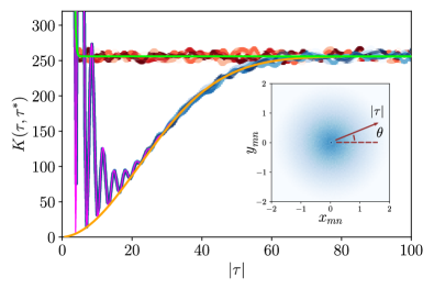
Figure 1: $K(\tau,\tau^{*})$ vs. $|\tau|$ for the GinUE and a Poissonian-random spectrum (defined above (5)) with matrix size $N=256$. Writing $\tau=|\tau|e^{i\theta}$, numerical simulations of GinUE (Poisson) for fixed $\theta=0$ to $\theta=\pi/2$ in steps of $\pi/4$ are plotted in blue colors (red colors) in multiple shades. The analytical solutions of $K_{\mathrm{GinUE}}$ (Eq. (3)) and $K_{\mathrm{Poi}}$ (Eq. (5)) are plotted as the purple and green lines on top of the numerical data. The connected part of $K_{\mathrm{GinUE}}$ (1st and 3rd terms in Eq. (3)) is plotted as the orange line. Inset: Two-dimensional histogram of $\{z_{mn}\equiv z_{m}-z_{n}\}$ of the GinUE for $N=1024$ where increasing values are plotted with deeper blue colors. Note that the bin at the origin is occupied by $N$ (diagonal) contributions of $\{z_{nn}=0\}$, and there is a dip around the origin due to level repulsion. The computation of DSFF for fixed $\theta$ as a function of $|\tau|$ is equivalent to the computation of SFF as a function of $|\tau|$ of $\{z_{m}\}$ projected onto the axis defined by $\theta$. The sample sizes are 5000 and 2000 for Poisson and GinUE respectively.

Spectral form factor. It is instructive to review the behaviour of SFF for closed quantum systems Haake (2010), with which DSFF shares several analogous features. Consider a closed quantum system described by a $N\times N$ Hermitian (or unitary) matrix with the density of states (DOS) $\rho(E)=\sum_{n}\delta(E-E_{n})$ where $E_{n}$ is the $n$-th eigenlevel (or eigenphase). Note that in our convention, $\int dE\,\rho(E)=N$. The correlation between eigenlevels can be quantified by the (so-called “2$\alpha$-point”) SFF, which is the ($\alpha$-th power of the) Fourier transform of two-level correlation function $\langle\rho(E)\rho(E+\omega)\rangle$, and can be directly defined as

$$K_{\alpha}(t):=\left\langle\,\left[\sum_{n,m}e^{-i(E_{n}-E_{m})t}\right]^{\alpha}\right\rangle\;,$$ (1)

where $\langle\cdot\rangle$ denotes the average over an ensemble of statistically similar systems. Importantly, SFF captures correlations between eigenlevels at all scales, including the level repulsion and spectral rigidity, while at the same time it is one of the simplest non-trivial and analytically tractable diagnostic of quantum chaos . Furthermore, SFF has recently been shown to capture novel signatures of quantum many-body physics like the deviation from RMT behaviour at early time (and consequently, the onset of chaos)  Kos et al. (2018); Bertini et al. (2018); Roy and Prosen (2020); Flack et al. (2020); Chan et al. (2018a, b); Friedman et al. (2019); Moudgalya et al. (2020); Garratt and Chalker (2020); Gharibyan et al. (2018); Chan et al. (2020, 2021); Cotler et al. (2017a, b); Saad et al. (2019); Gharibyan et al. (2018); Garratt and Chalker (2020); Bertini et al. (2021); Winer and Swingle (2020); Šuntajs et al. (2020). For integrable systems with Poisson statistics, we have $K_{1}(t)=N$ for $t$ larger than a timescale set by the inverse width of DOS. For quantum chaotic systems without symmetries, the generic behaviour of SFF can be understood by studying the Gaussian unitary ensemble (GUE). SFF for GUE initially decays and then grows linearly until the Heisenberg time, $t_{\mathrm{Hei}}$, after which $K(t)=N$ reaches a plateau. Qualitatively, this is referred to as the “dip-ramp-plateau” behaviour. The form of the early time decay is due to the (non-universal) form of the DOS, while the linear ramp reflects the phenomenon of spectral rigidity. $t_{\mathrm{Hei}}$ is proportional to the inverse of the mean level spacing, and it encodes the largest physically relevant time scale of the system.

Dissipative spectral form factor. For a $N\times N$ non-Hermitian matrix with complex spectra, the SFF is exponentially growing or decaying in time due to the imaginary parts of the complex eigenvalues. Moreover, traditional methods like the Green’s function approach fail due to non-analyticity of the Green’s function. To circumvent these problems, we consider 2D DOS, $\rho(z)=\sum_{n}\delta(x-x_{n})\delta(y-y_{n})$, where $z=x+iy$, $x_{n}=\mathrm{Re}\,z_{n}$, $y_{n}=\mathrm{Im}\,z_{n}$, and $z_{n}=x_{n}+iy_{n}$ is the $n$-th complex eigenvalue. We introduce the (“$2\alpha$-point”) DSFF as the ensemble average of the ($\alpha$-th power of the) 2D Fourier transform of the two-level correlation function $\langle\rho(x,y)\rho(x+\omega,y+\omega^{\prime})\rangle$. We directly define DSFF as

$$K_{\alpha}(t,s):=\left\langle\left[\sum_{m,n}e^{i(x_{n}-x_{m})t+i(y_{n}-y_{m})s}\right]^{\alpha}\right\rangle\;,$$ (2)

where $t$ and $s$ are two “time” variables conjugate to the $x_{n}-x_{m}$ and $y_{n}-y_{m}$ respectively. Importantly, the correlation between both the real and imaginary parts of two given complex eigenvalues now contributes to DSFF as phases. Notice that if the spectrum is real, DSFF is effectively reduced to SFF as a function of $t$ for all $s$. To obtain an intuition of how DSFF behaves, we write $\vec{z}_{mn}\equiv(x_{mn},y_{mn})\equiv(x_{m}-x_{n},y_{m}-y_{n})$, and $\vec{\tau}\equiv(t,s)=(|\tau|\cos\theta,|\tau|\sin\theta)$. The DSFF can now be written as $K_{\alpha}(t,s)=\left\langle\left[\sum_{m,n}e^{i\vec{z}_{mn}\cdot\vec{\tau}}\right]^{\alpha}\right\rangle\;,$ which allows a natural interpretation in the complex plane: At fixed $\theta$ and as a function of $|\tau|$, ($2\alpha$-point) DSFF is the ($\alpha$-point) SFF of the projection of $\{z_{m}\}$ onto the radial axis specified by angle $\theta$ (illustrated in Fig.1 inset). Reverting back to the notation with complex numbers, we define complex time, $\tau=t+is$ and write DSFF as ${K}_{\alpha}(\tau,\tau^{*})=\left\langle\left|\sum_{n}e^{i(z_{n}\tau^{*}+z_{n}^{*}\tau)/2}\right|^{2\alpha}\right\rangle$, For ensembles where the two-point correlation function $\langle\rho(z_{1})\rho(z_{2})\rangle$ is known, DSFF at $\alpha=1$ can be written as an integral $K_{1}=\int d^{2}z_{1}d^{2}z_{2}\,\langle\rho(z_{1})\rho(z_{2})\rangle\,e^{i(z_{1}\tau^{*}+z_{1}^{*}\tau-z_{2}^{*}\tau-z_{2}\tau^{*})/2}\;.$ For the rest of the paper, we will drop the subscript and focus on the simplest and most relevant case $\alpha=1$.

Dissipative quantum chaotic systems. We use the GinUE as a minimal model of the dissipative quantum chaotic systems. The joint probability distribution function of eigenvalues of GinUE is known exactly, and the correlation function of eigenvalues can be expressed in terms of the kernel Ginibre (1965), $\mathcal{K}(z_{1},z_{2})=\frac{N}{\pi}e^{-\frac{N}{2}(|z_{1}|^{2}+|z_{2}|^{2})}\sum_{\ell=0}^{N-1}\frac{(Nz_{1}z_{2}^{*})^{\ell}}{\ell!}\;.$ The 1-point correlation function, i.e. the DOS, is given by $\langle\rho(z)\rangle=\mathcal{K}(z,z)$, and the kernel is normalized such that $\int d^{2}z\,\langle\rho(z)\rangle=\int d^{2}z\,\mathcal{K}(z,z)=N$. Note that the DOS is isotropic, and is asymptotically, as $N\to\infty$, flat on a unit disc $|z|<1$ and vanishing outside. The 2-point correlation function is $\langle\rho(z_{1})\rho(z_{2})\rangle=\mathcal{K}(z_{1},z_{1})\delta(z_{1}-z_{2})+\mathcal{K}(z_{1},z_{1})\mathcal{K}(z_{2},z_{2})-\left|\mathcal{K}(z_{1},z_{2})\right|^{2}$. We will refer to the above three terms as the contact, disconnected and connected term respectively. Using $\langle\rho(z_{1})\rho(z_{2})\rangle$, we compute (2) by expanding the exponential factors, and using the fact that the integrals over the phases of $z_{1}$ and $z_{2}$ kill all terms in the sum except the ones depending on $|z_{1}|$ and $|z_{2}|$. This gives

$$K_{\mathrm{GinUE}}(\tau,\tau^{*})=N+N^{2}\,_{1}F_{1}\left(N+1;2;-\frac{\left|\tau\right|^{2}}{4N}\right)^{2}-\sum_{n,m=0}^{N-1}\frac{(\max(m,n)!)^{2}}{n!m!(\left|m-n\right|!)^{2}}\,_{1}F_{1}\left(\max(m,n)+1;\left|m-n\right|+1;-\frac{\left|\tau\right|^{2}}{4N}\right)^{2},$$ (3)

where we have listed the three terms in the same ordering as in the 2-point correlation function. ${}_{1}F_{1}(a,b;z)=\sum_{n=0}^{\infty}a^{(n)}z^{n}/b^{(n)}n!$ is the Kummer confluent hypergeometric function, where $a^{(n)}$ is the rising factorial. Keeping the leading contributions in $N$, Eq. (3) becomes

$$K_{\mathrm{GinUE}}(\tau,\tau^{*})=N+N^{2}\frac{4J_{1}(\left|\tau\right|)^{2}}{\left|\tau\right|^{2}}-N\exp\left(-\frac{|\tau|^{2}}{4N}\right)\,,$$ (4)

where $J_{\mu}(x)$ is the Bessel function of the first kind. Along with Eq. (3), Eq. (4) forms our main result, as they capture the universal spectral correlations of dissipaitve quantum chaotic systems. Firstly, note that $K_{\mathrm{GinUE}}(\tau,\tau^{*})$ only depends on the absolute value of $\tau$, i.e. DSFF is manifestly rotational symmetric in complex time (see Fig. 1). Secondly, the qualitative behaviour of DSFF as a function of $|\tau|$ for dissipative quantum systems shows a dip-ramp-plateau structure, analogous to SFF for closed quantum systems: At early time $|\tau|\lesssim\tau_{\mathrm{edge}}$, DSFF dips from $K(0,0)=N^{2}$ with a form dominated by the disconnected piece (3); At intermediate time $\tau_{\mathrm{edge}}\lesssim|\tau|\lesssim\tau_{\mathrm{Hei}}$, DSFF increases quadratically $K_{\rm GinUE}\simeq|\tau|^{2}/4$ with precise form given by the sum of hypergeometric functions, or the Gaussian function for large $N$, until it reaches late time $\tau_{\mathrm{Hei}}\lesssim|\tau|$ with $\tau_{\mathrm{Hei}}\sim\sqrt{N}$, where DSFF reaches a plateau at $N$. Note that the DSFF GinUE ramp behaviour is drastically different from the corresponding SFF GUE behaviour, which is linear in time. Thirdly, in analogy to SFF, the connected term in DSFF captures the spectral rigidity in the complex spectral plane. As apparent from the functional form of the connected term, we see that the Heisenberg time scales as the inverse of mean level spacing (in the complex plane), $\tau_{\mathrm{Hei}}=O(\Delta^{-1})=O(\sqrt{N})$. sup Again, this is in contrast to the corresponding Heisenberg time scaling for SFF, which scales as $N$. Fourthly, the non-oscillatory part of the disconnected term asymptotically scales as $N^{2}|\tau|^{-3}$. Setting the time $\tau_{\mathrm{edge}}$ where disconnected and connected contributions are of the same order, we find $\tau_{\mathrm{edge}}=O(N^{2/5})$. Note that as a function of $|\tau|$, the GinUE disconnected term of DSFF coincides with the GUE disconnected term of SFF, due to the fact that the projection of the DOS along the axis defined by $\theta$ exhibits a semi-circle shape, like the DOS of GUE. Fifthly, according to the interpretation described above, DSFF at fixed $\theta$ is equivalent to the SFF of the projected spectrum $\{z_{m}\}$ along the axis defined by $\theta$. While there is level repulsion in the 2D complex plane, there are accidental degeneracies between distanced pairs of eigenvalues in the set of projected $\{z_{m}\}$, and remarkably, the lack of level repulsion along the projection axis makes up for the difference between SFF of GUE, which has linear ramp in $t$ with $t_{\mathrm{Hei}}=O(N)$, and DSFF of GinUE which has a quadratic ramp in $|\tau|$ with $\tau_{\mathrm{Hei}}=O(\sqrt{N})$.

Lastly, the GinUE DSFF result can be interpreted via the mapping between GinUE and 2D log-potential Coulomb gas. DSFF is equivalent to the 2D static structure factor (SSF), defined as the Fourier transform of density-density fluctuation, where the complex energy and the complex time in (2) take the roles of position and wavevector $\vec{k}$. For the Coulomb gas, with the assumption of “perfect screening”, SSF is argued to have an asymptotic behaviour of $|\vec{k}|^{2}$ for small $|\vec{k}|$ Baus and Hansen (1980), which is consistent with the quadratic increase $|\tau|^{2}$ for large $N$ in (4). Furthermore, a system is hyperuniform if its SSF vanishes as $|\vec{k}|$ tends to zero. This implies that density fluctuation is suppressed at very large length scales Torquato and Stillinger (2003); Torquato (2018). This leads us to interpret that the spectrum of GinUE is a 2D gas that displays hyperuniformity with a quadratic power-law form.

The numerical data and analytical solutions are plotted in Fig. 1 for $N=256$ with excellent agreement. We further computed DSFF for the real (GinOE) and quaternion real (GinSE) Ginibre ensembles sup . The rotational symmetry of $K$ in $\tau$ is broken, since eigenvalues of quaternion real (real) ensemble (are either real or) come in complex conjugate pairs, which leads to special behaviour of $z_{mn}$ near $\theta=0,\pi/2$ sup . We define critical angles ${\theta^{*}_{0}}$ and ${\theta^{*}_{\pi/2}}$ such that DSFF of GinOE and GinSE coincide with the one of GinUE for $\theta\in[{\theta^{*}_{0}},\pi/2-{\theta^{*}_{\pi/2}}]$. We numerically show and heuristically argue that ${\theta^{*}_{\phi}}\propto N^{-1/2}$ with the only exception of ${\theta^{*}_{\pi/2}}\propto N^{-0.56}$ for GinSE due to the lack of “projected degeneracies” sup . We therefore conclude that, in large $N$, GinOE and GinSE coincide with the GinUE behaviour except for the angle $\theta=0$ and $\pi/2$. This is consistent with the fact that spectral correlations of these ensembles coincide with GinUE for eigenvalues away from the real axis Lehmann and Sommers (1991); Forrester and Nagao (2007); Borodin and Sinclair (2009); Akemann and Kanzieper (2007); Sommers and Wieczorek (2008).

Dissipative integrable systems. We model the spectrum of dissipative quantum integrable systems with a set of uncorrelated normally distributed complex eigenvalues. The DOS is $\langle\rho(z)\rangle=N(2\pi)^{-1}e^{-|z|^{2}/2}$ with $\int d^{2}z\,\langle\rho(z)\rangle=N$. The 2-point correlation function is $\langle\rho(z_{1})\rho(z_{2})\rangle=\langle\rho(z_{2})\rangle\delta(z_{1}-z_{2})+\frac{N(N-1)}{N^{2}}\langle\rho(z_{1})\rangle\langle\rho(z_{2})\rangle$. The DSFF can be evaluated as

$$K_{\mathrm{Poi}}(\tau,\tau^{*})=N+N(N-1)e^{-|\tau|^{2}}\;.$$ (5)

We see that DSFF for Poissonian random spectrum takes a constant value of $N$ except for a small region of complex time near the origin. The constant value $N$ is due to the diagonal contribution from DSFF, and the deviation from $N$ is due to the disconnected part and depends on the details of the DOS. The numerical data and analytical solution are plotted in Fig. 1 for $N=256$ with excellent agreement.

Dissipative quantum kicked top model. A simple but rich example of quantum systems that exhibit chaotic and integrable behaviours is the quantum kicked top (QKT) model Grobe et al. (1988); Haake et al. (1987); Gorin et al. (2006) which has been experimentally realized in Smith et al. (2004). The unitary evolution of QKT is governed by the Hamiltonian Grobe et al. (1988),

$$H(t)=pJ_{z}+\frac{k_{0}}{2j}J^{2}_{z}+\frac{k_{1}}{2j}J_{y}^{2}\sum_{n=-\infty}^{\infty}\delta(t-n)\;,$$ (6)

where $\vec{J}=(J_{x},J_{y},J_{z})$ are angular momentum operators that act on a single spin-$j$ particle and obey $[J_{\alpha},J_{\beta}]=i\epsilon_{\alpha\beta\gamma}J_{\gamma}$, $\alpha,\beta,\gamma\in\{x,y,z\}$. The first two terms describe the precession of the spin. The third term describes a periodic kick at integer time $n$. We introduce the dissipation by considering the action of the quantum map in the Kraus form $\Phi(\rho)=\sum_{a}K_{a}e^{-iH}\rho e^{iH}K^{\dagger}_{a}$, where $K_{1,2}=(J_{x}\pm iJ_{y})/\sqrt{j(j+1)}$ and $K_{3}=\sqrt{2}J_{z}/\sqrt{j(j+1)}$ such that the constraint $\sum_{a}K^{\dagger}_{a}K_{a}=\mathbb{1}$ is satisfied to ensure trace preservation and complete positivity Nielsen and Chuang (2010). The time evolved density matrix is obtained by a successive action of $\Phi$, i.e. $\rho(t)=\Phi^{t}(\rho)$. We represent $\Phi$ as a superoperator, i.e. $\Phi=\sum_{a}(K_{a}\otimes K^{*}_{a})(U\otimes U^{*})$, where $U=\mathcal{T}\exp[-i\int_{0}^{1}dt\,H(t)]$ and $\mathcal{T}$ is the time-ordering. Note that the total angular momentum $\vec{J}^{2}$ and the parity are conserved and we will therefore study the restricted Hilbert space of size roughly half of $(2j+1)^{2}$. We analyse the DSFF of the spectrum of $\Phi$ in the symmetric subspace. Note that the spectrum is symmetric across the real axis sup . As shown in Fig. 2, as we turn on and off the kick parameter $k_{1}$, the DSFF coincides with the GinOE (for all angles sup ) and Poisson behaviour with excellent agreement. Note that the DSFF of the corresponding Liouvillian operators of the Lindblad form of the QKT also converges to GinOE DSFF behaviour.

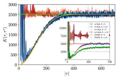
Figure 2: Main: DSFF of QKT with dissipation for $j=35$ and Gaussianly-distributed $p\in\mathcal{N}(2,2/3)$ and $k_{0}\in\mathcal{N}(10,3)$. The blue (red) lines in different shades are for DSFF of QKT with the kick with $k_{1}=8$ (without the kick with $k_{1}=0$) for fixed $\theta\in[\pi/16,7\pi/16]$ in steps of $\pi/16$. The two cases fit the connected part of GinUE (orange line) and Poisson (green line) predictions as expected. Inset: DSFF of QKT and GinOE for angles $\theta=0,\pi/2$ sup . The sample sizes for QKT with and without the kick are 2500 and 4300 respectively.

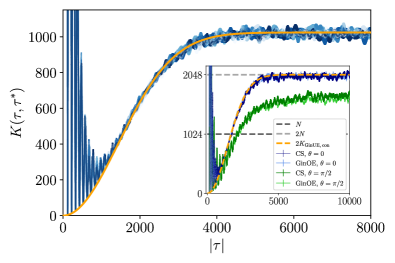
Figure 3: Main: DSFF of the random classical stochastic ensemble induced by CUE for $N=1024$ with sample size 5000. The blue colors are for fixed $\theta\in[\pi/16,7\pi/16]$ in steps of $\pi/16$. The data can be fitted with the connected part of GinUE (orange line). Inset: DSFF for CS and GinOE at angles $\theta=0,\pi/2$ sup .

Classical stochastic systems. Another interesting class of non-Hermitian matrices are classical stochastic matrices or Markov chains, which are matrices with real positive entries and with each column summing to unity. A particular way to generate an ensemble of random stochastic matrices is to consider matrix $S$ with entries $S_{ij}={|M_{ij}|^{2}}/{\sum_{i}|M_{ij}|^{2}}$, where $M_{ij}$ is a matrix chosen from a certain matrix ensemble. We consider classical stochastic (CS) matrices induced from two random ensembles: the circular unitary ensemble (CUE) (whose induced stochastic ensemble is called the uni-stochastic ensemble) and the GinUE. Unistochastic matrices arise in the context of quantum graphs Tanner (2001, 2000); Gnutzmann and Smilansky (2006) and in the theory of majorization and characterization of quantum maps Marshall et al. (2011); Nielsen (1999, 2000); Hammerer et al. (2002). By the Perron-Frobenius theorem, the stochastic matrices have leading eigenvalues of unity, and the spectra are again symmetric across the real axis Zyczkowski et al. (2003); sup . We plot the DSFF for the uni-stochastic ensemble in Fig. 3 and the other GinUE-induced ensemble in the supplementary material sup . For both ensembles, the DSFF behaviour coincides with the GinOE behaviour (for all angles sup ) with excellent agreement.

Discussion. We have proposed and exactly computed DSFF for GinUE and a Poissonian-random spectrum as minimal models of dissipative quantum chaotic and integrable systems. In particular, we show that DSFF for GinUE has a dip-ramp-plateau behaviour with a quadratic ramp, and numerically demonstrated the universality of the result with the example of QKT and random classical stochastic ensembles. This work open up many exciting directions: DSFF can be used to classify dissipative quantum chaotic systems in different universality and symmetry classes, beyond the nearest-neighbour spacing distribution studied previously Magnea (2008); Kawabata et al. (2019); Bernard and LeClair (2002); Hamazaki et al. (2020), and to unveil deviation of open quantum many-body systems from RMT behaviours at early time (cf. Kos et al. (2018); Bertini et al. (2018); Roy and Prosen (2020); Flack et al. (2020); Chan et al. (2018a, b); Friedman et al. (2019); Moudgalya et al. (2020); Garratt and Chalker (2020); Gharibyan et al. (2018); Chan et al. (2020)). In particular, it can be used to investigate the spectral properties across the measurement-induced phase transition Skinner et al. (2019); Li et al. (2018, 2019); Chan et al. (2019); Bao et al. (2020); Jian et al. (2020); Zabalo et al. (2020). These directions will be discussed in an upcoming work Li et al. .

Lastly, note that DSFF contrasts with a related observable called dissipative form factor Can (2019) (DFF) in several ways: DFF is a one-parameter function defined for the (Lindblad) superoperators, and the correlation between the imaginary parts of eigenvalues contribute to the DFF as an exponential factor (as supposed to a phase in DSFF). This makes DFF useful in capturing the scaling of the spectral gap, while DSFF is beneficial in unraveling the correlation between eigenvalues in the bulk of the spectrum.

Acknowledgement. We are thankful to Fiona Burnell, David Huse, Abhinev Prem, Shinsei Ryu, Lucas Sá, Shivaji Sondhi and Salvatore Torquato for helpful discussions. AC is particularly grateful to Tankut Can for pointing out the connections to static structure factor and hyperuniformity, and to John Chalker and Andrea De Luca for collaborations on related projects. AC is supported by fellowships from the Croucher foundation and the PCTS at Princeton University. TP acknowledges ERC Advanced grant 694544-OMNES and ARRS research program P1-0402.

Supplementary Material
Spectral statistics of non-Hermitian matrices and dissipative quantum chaos

In this supplementary material we provide additional details about:

1. Dissipative spectral form factor (DSFF) for additional ensembles and discussion of DSFF at $\theta=0,\pi/2$

2. Spectra of single realizations

3. Density of states

4. Scaling of Heisenberg time $\tau_{\mathrm{Hei}}$

5. DSFF for modified spectra with “projected degeneracies”

6. DSFF for $\theta$ near $0$ and $\pi/2$

7. Scaling of the critical angle $\theta^{*}$

   • Definition of $\theta^{*}$

   • Scaling of $\theta^{*}$

   • Arguments for the scaling of $\theta^{*}$

Appendix A DSFF for additional ensembles and discussion of DSFF at $\theta=0,\pi/2$

Here we present the DSFF for real Ginibre ensemble (GinOE), quaternion real Ginibre ensemble (GinSE) and ensembles of classical stochastic matrices induced by GinUE in Fig. S1 left, Fig. S1 right and Fig. S2 respectively. To discuss DSFF at $\theta=0$ and $\pi/2$, we recall the interpretation of DSFF discussed in the main text below Eq. (2): At fixed $\theta$ and as a function of $|\tau|$, DSFF is the SFF of the projection of complex eigenvalues onto the radial axis specified by angle $\theta$. At $\theta=0$, a spectrum that is symmetric across the real axis has a rough 2-fold degeneracy in the projected set of eigenvalues (it is not an exact 2-fold degeneracy due to the real eigenvalues, which do not come in pairs). This gives an explanation of the approximate fit of $2K_{\mathrm{GinUE}}$ along $\theta=0$ for GinOE, GinSE, QKT, the ensembles of classical stochastic matrices (see insets of Fig. S1, 2, 3 and S2 respectively). Along $\theta=\pi/2$, the real eigenvalues will be exactly degenerate after the projection onto the radial axis defined by $\theta=\pi/2$, which would lead to a different large-$|\tau|$ value for DSFF. This fact is demonstrated when we compare DSFF of GinOE and GinSE at $\theta=\pi/2$: For GinOE, spectra contain real eigenvalues (see Fig. S3 middle), and DSFF at $\theta=0$ approaches a value larger than matrix size $N$, while for GinSE, spectra have no real eigenvalues (see Fig. S3 right) and DSFF at $\theta=0$ approaches $N$. We leave the study of DSFF behaviour near $\theta=0,\pi/2$ for future investigations.

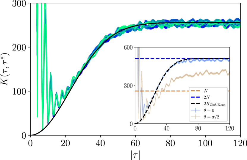
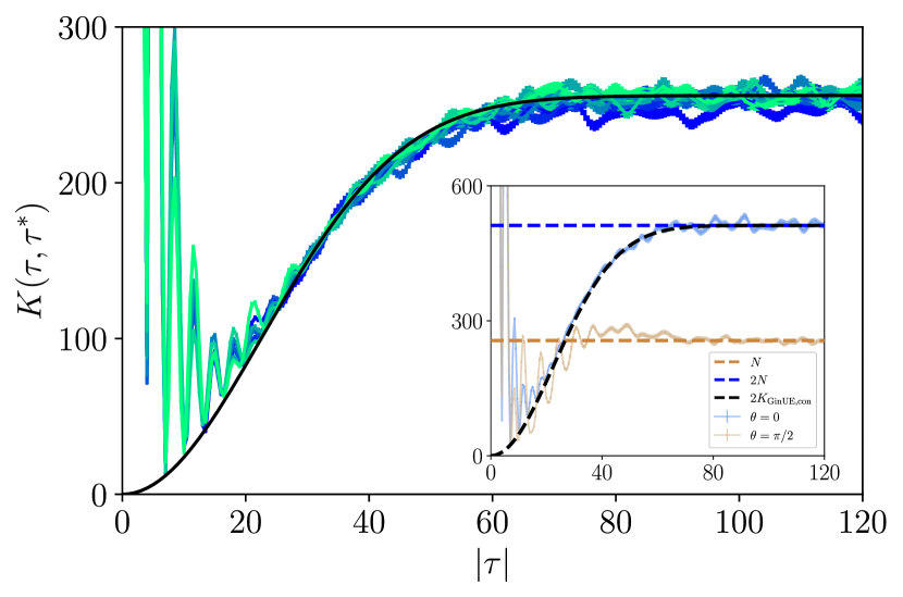
Figure S1: Main: DSFF of the GinOE (left) and GinSE (right) for $N=256$ with sample sizes 5000. The blue/green colors are for fixed $\theta\in[\pi/16,7\pi/16]$ in steps of $\pi/16$. The data are fitted with the connected part of GinUE (black line). Inset: DSFF for angle $\theta=0,\pi/2$. We find that DSFF at $\theta=0$ can be fitted with twice the connected part of DSFF for GinUE.

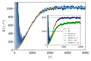
Figure S2: Main: DSFF of the ensembles of classical stochastic matrices induced by GinUE for matrix size $N=1024$ and sample size 5000. The blue colors are for fixed $\theta\in[\pi/16,7\pi/16]$ in steps of $\pi/16$. The data is fitted with the connected part of GinUE (orange line). Inset: DSFF for CS and GinOE at angles $\theta=0,\pi/2$. We find that DSFF at $\theta=0$ can be fitted with twice the connected part of DSFF for GinUE.

Appendix B Spectra of single realizations

In this section, we provide the plots of spectra of single realizations of the ensembles considered in the main text, namely, the DOS of GinUE, GinOE, GinSE (Fig. S3), QKT with and without the kick (Fig. S4), ensembles of classical stochastic matrices induced by CUE and GinUE (Fig. S5).

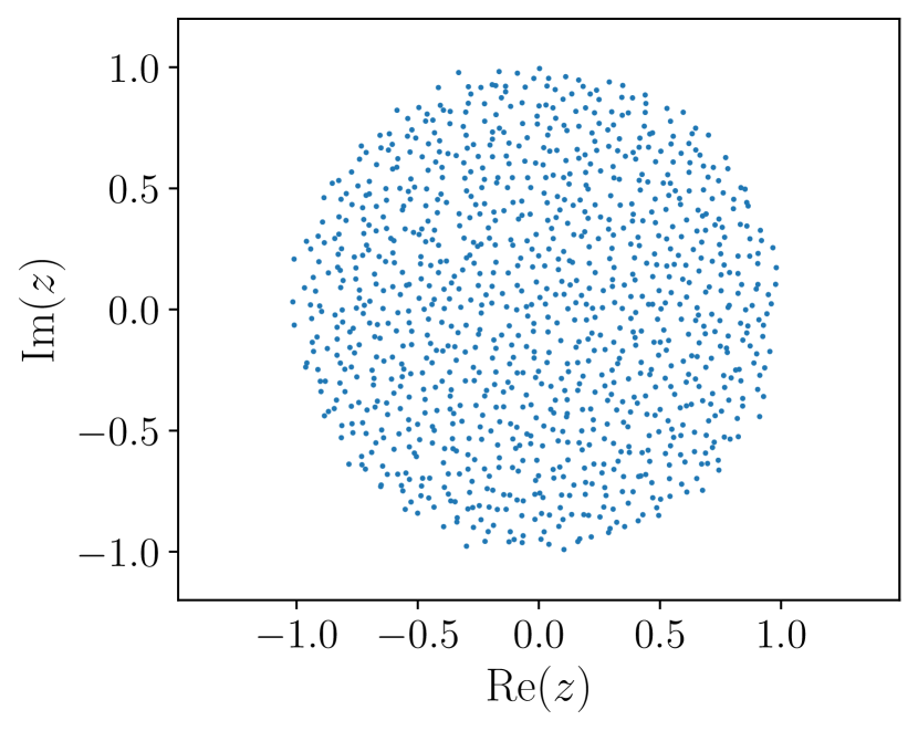
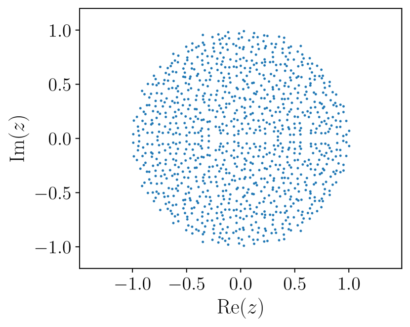
Figure S3: Spectra of single realizations of the GinUE (left), GinOE (middle) and GinSE (right) with matrix size $N=1024$. Each set of eigenvalues lies within the unit circle in the complex plane, shows level repulsion, and has a uniform distribution away from the edge of the circle (and the real axis for GinOE and GinSE). For GinOE (GinSE), there is a finite (zero) eigevalue density along the real axis (cf. Fig. S6).

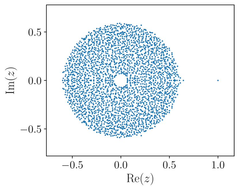
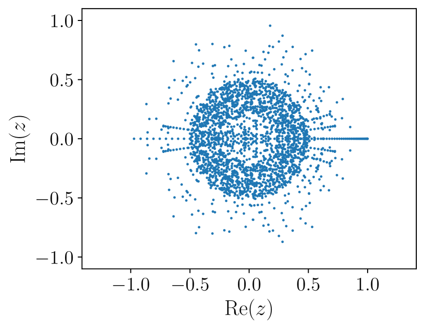
Figure S4: Spectra of single realizations of the QKT with dissipation for $j=35$, Gaussianly-distributed $p\in\mathcal{N}(2,2/3)$ and $k_{0}\in\mathcal{N}(10,3)$. The left and right figures are for the QKT with the kick with $k_{1}=8$, and without the kick with $k_{1}=0$ respectively. Both spectra have leading eigenvalues of unity and are symmetric across the real axis. QKT with the kick (without the kick) is dissipative quantum chaotic (integrable), and its DSFF behaviour converges to the one of GinUE (Poisson) (see Fig. 2 in the main text).

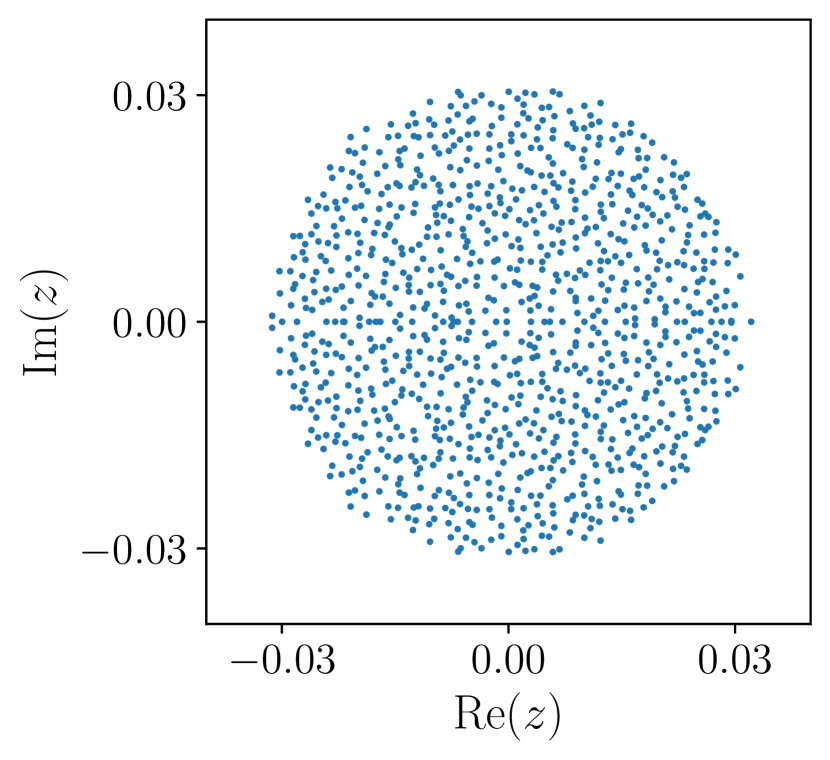
Figure S5: Spectra of single realizations of the ensembles of classical stochastic matrices induced from the CUE (left) and GinUE (right) with matrix size $N=1024$. There is a leading eigenvalue of unity (not shown) and the spectrum is symmetric across the real axis. The spectrum exhibits level repulsion and its DSFF converges to the one of GinUE (see Fig. 3 and S2).

Appendix C Density of states

In this section, we provide the heat maps of the density of states for the ensembles considered in the main text, namely, the DOS of GinUE, GinOE, GinSE (Fig. S6), QKT with and without the kick (Fig. S7), ensembles of classical stochastic matrices induced by CUE and GinUE (Fig. S8).

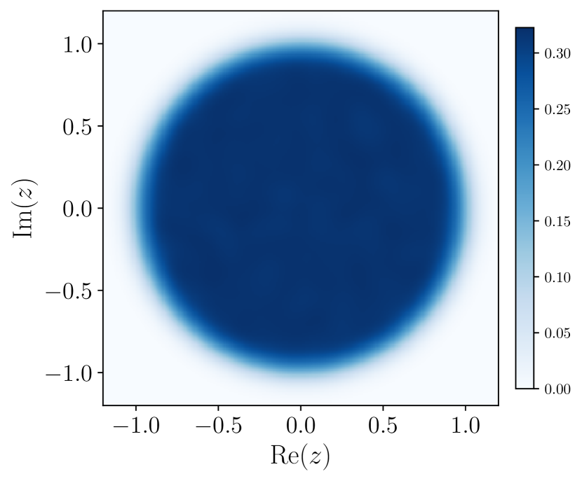
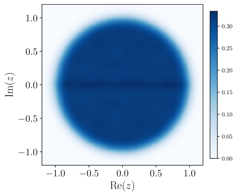
Figure S6: DOS of GinUE (left), GinOE (middle) and GinSE (right) with matrix size $N=256$ and sample size 100. Each set of eigenvalues lies within the unit circle in the complex plane, shows level repulsion, and has a uniform distribution away from the edge of the circle (and the real axis for GinOE and GinSE). For GinOE (GinSE), there is a finite (zero) eigevalue density along the real axis (cf. Fig. S3).

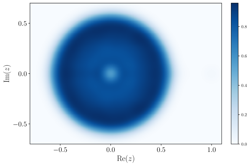
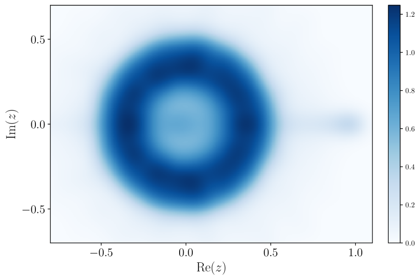
Figure S7: DOS of the QKT with dissipation for $j=35$, and Gaussianly-distributed $p\in\mathcal{N}(2,2/3)$ and $k_{0}\in\mathcal{N}(10,3)$. The left and right figures are for the QKT with the kick with $k_{1}=8$, and without the kick with $k_{1}=0$ respectively. Both DOS figures are obtained by averaging over a sample of 10 realizations.

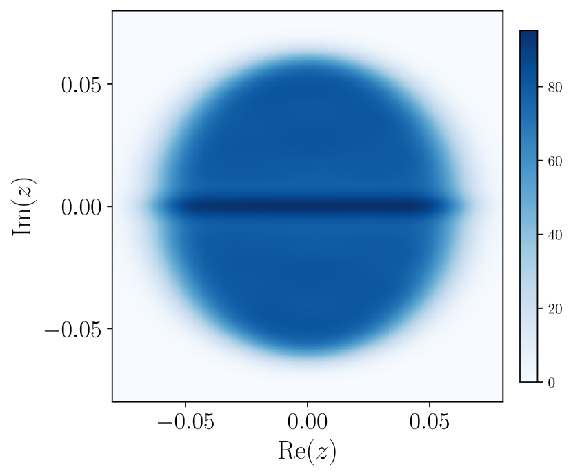
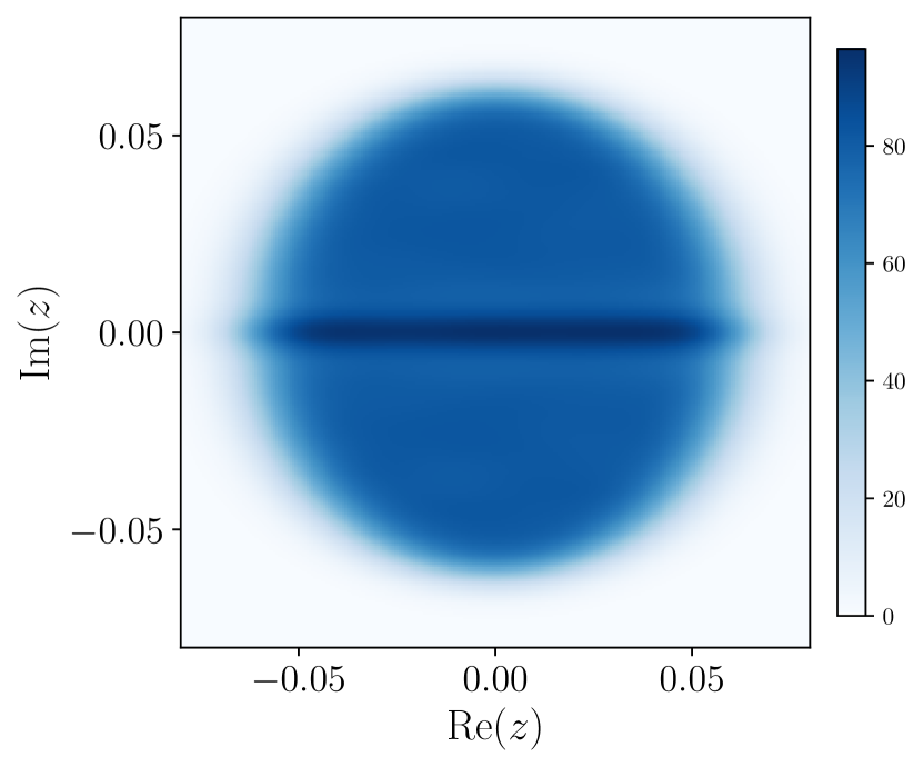
Figure S8: DOS of ensembles of classical stochastic matrices induced from the CUE (left) and the GinUE (right) with matrix size $N=256$ and sample size 1000.

Appendix D Scaling of Heisenberg time $\tau_{\mathrm{Hei}}$

In this section, we provide the scalings of the Heisenberg time, $\tau_{\mathrm{Hei}}$, for GinUE, GinOE, GinSE (Fig. S9), QKT with the kick (Fig. S10), and ensembles of classical stochastic matrices (Fig. S11). We show that $\tau_{\mathrm{Hei}}$ scale as the inverse level spacing $\Delta^{-1}\propto\sqrt{N}$, as predicted by the GinUE results. Our fitting protocol is as follows. We consider the fucntional form of the analytical solution of the connected DSFF for GinUE (the first and third terms in Eq. (4)) given by $f(|\tau|,N)=N-N\exp(-A(N)|\tau|^{2})$, where $N$ and $A(N)$ are the matrix size (restricted to the relevant symmetry sector) and a fitting parameter respectively. We numerically identify the time scale $\tau^{*}$ after which the contribution of disconnected DSFF is small compare to the connected DSFF. We fit $f(|\tau|,N)$ with the data for $|\tau|>\tau^{*}$ for multiple $N$ and extract $A(N)$. We plot $\tau_{\mathrm{Hei}}\propto A(N)^{1/2}$ vs. $\Delta^{-1}$ in the log-log scale, and find a linear fit.

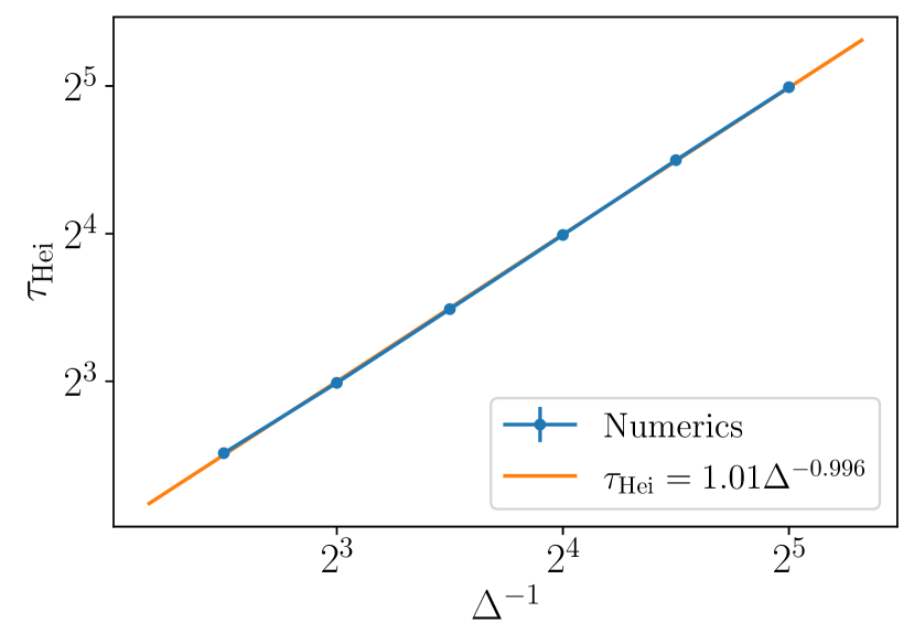
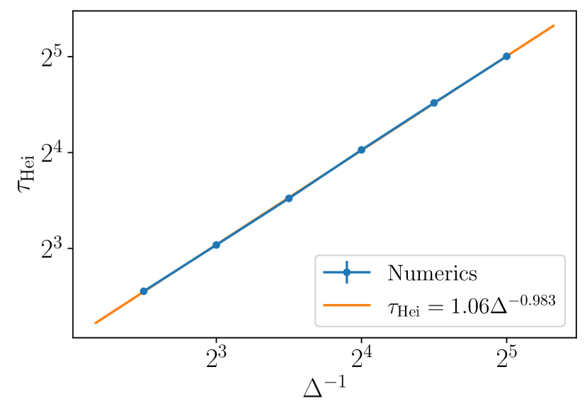
Figure S9: Heisenberg time $\tau_{\mathrm{Hei}}$ vs. inverse level spacing $\Delta^{-1}$ for GinUE (left), GinOE (middle) and GinSE (right). We see that $\tau_{\mathrm{Hei}}$ scales as $\tau_{\mathrm{Hei}}\propto\Delta^{-1}\propto\sqrt{N}$, as described by the analytical results from GinUE. Note that the error bars are smaller than the data points.

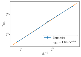
Figure S10: Heisenberg time $\tau_{\mathrm{Hei}}$ vs. inverse level spacing $\Delta^{-1}$ for the QKT with dissipation for $j=35$, $k_{1}=8$, $p\in\mathcal{N}(2,2/3)$ and $k_{0}\in\mathcal{N}(10,3)$. The Heisenberg time scales as $\tau_{\mathrm{Hei}}\propto\Delta^{-1}\propto\sqrt{N}$, as described by the GinUE results. Note that the error bars are smaller than the data points.

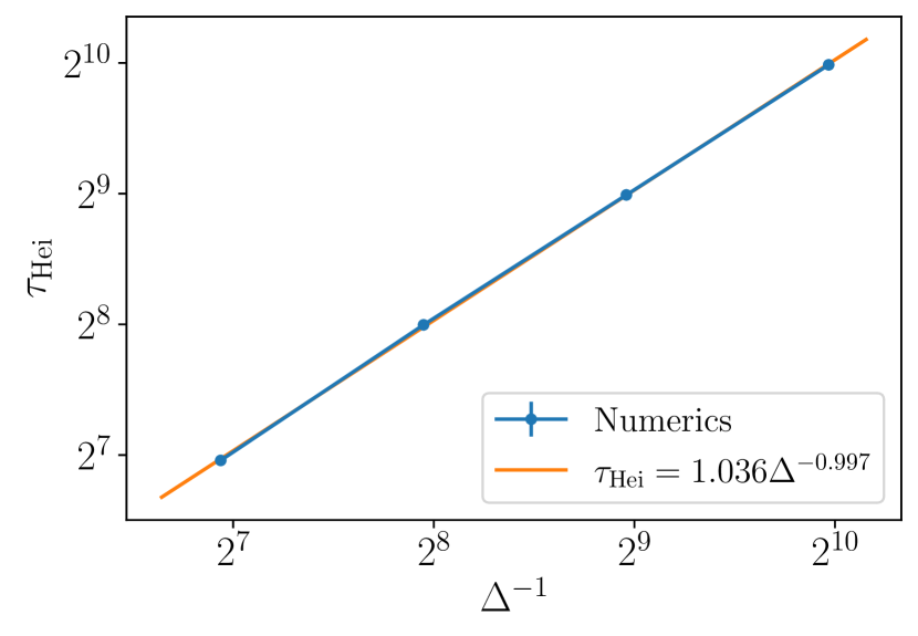
Figure S11: Heisenberg time $\tau_{\mathrm{Hei}}$ vs. inverse level spacing $\Delta^{-1}$ for ensembles of classical stochastic matrices induced from the CUE (left) or GinUE (right). Note that $\Delta^{-1}\propto\sqrt{N}/r(N)$ where $N$ and $r(N)$ are the matrix size and radius of the bulk of the DOS. For both cases, the Heisenberg time scales as $\tau_{\mathrm{Hei}}\propto\Delta^{-1}\propto\sqrt{N}/r(N)$, as described by the GinUE results. Note that the error bars are smaller than the data points.

Appendix E DSFF for modified spectra with “projected degeneracies” removed

The spectra of GinOE, QKT and CS contain complex conjugate pairs of eigenvalues and real eigenvalues, while the one of GinSE contain complex conjugate pairs only. These features lead to degeneracies in the set of eigenvalues projected along the axis defined by $\theta$, the “projected degeneracies” (c.f. interpretation of DSFF in the main text), which in turn make the DSFF behaviour special near $\theta=0,\pi/2$. Here we investigate the behaviour of DSFF of the modified spectra of GinOE and GinSE in Fig. S12 and Fig. S13 respectively.

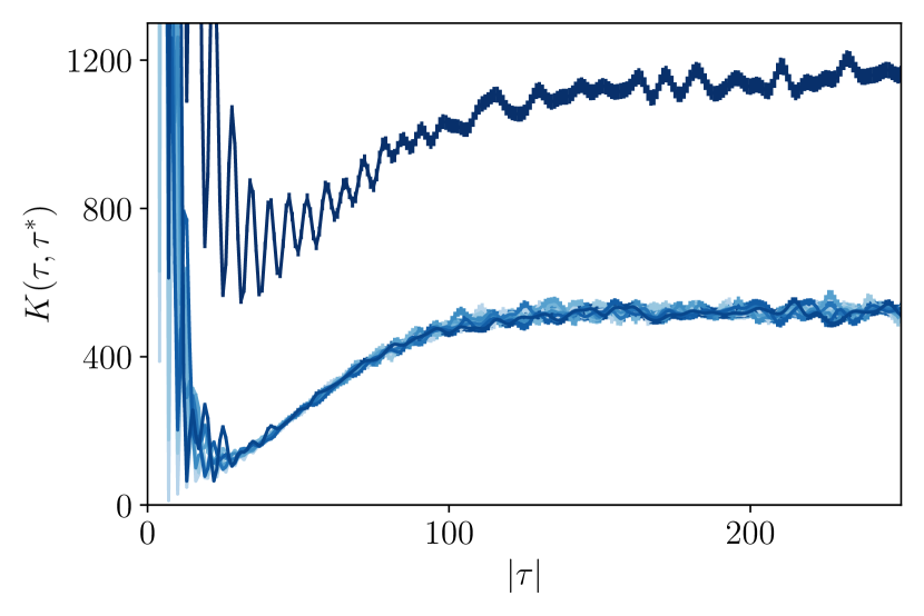
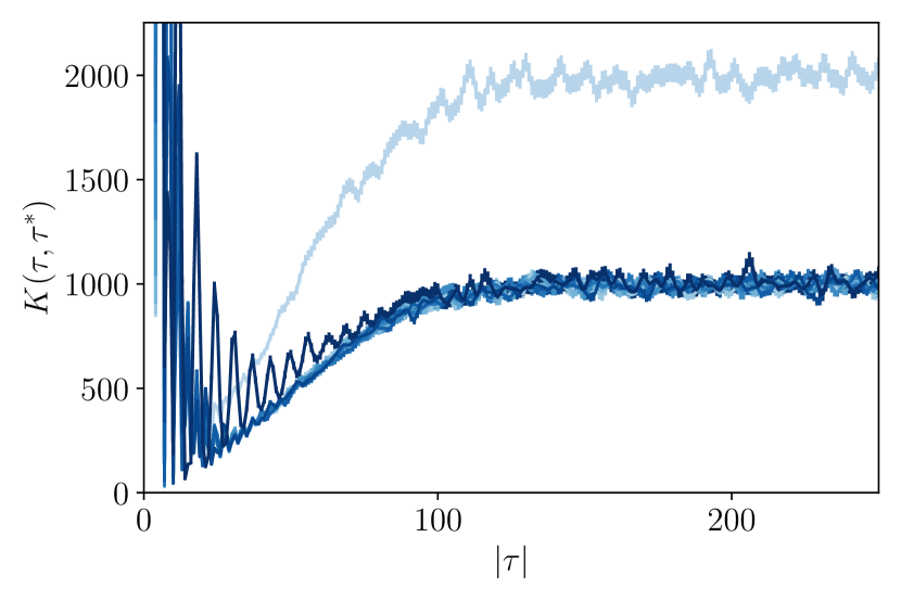
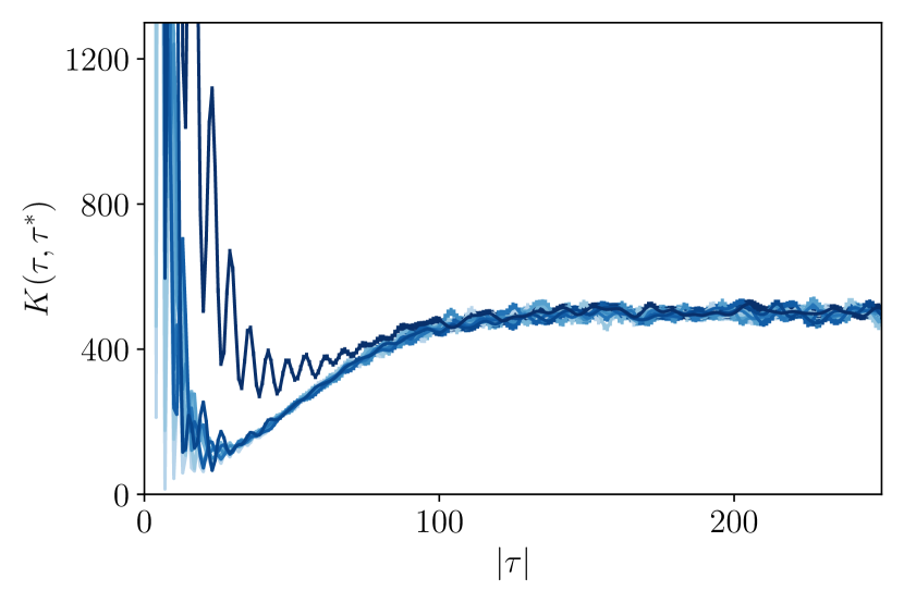
Figure S12: DSFF $K(\tau,\tau^{*})$ against $|\tau|$ at different values of $\theta$ from $0$ to $\pi/2$ in steps of $\pi/16$ (from light to dark blue) for the following cases: (i) GinOE with bottom half of the complex plane removed but with real eigenvalues kept (left); (ii) GinOE with real eigenvalues removed but with the bottom half plane kept (middle); and (iii) GinOE with both the real eigenvalues and the bottom half plane removed (right). We see that without the eigenvalues in the bottom half plane ((i) and (iii)), DSFF at $\theta=0$ (light blue) behaves like the one at $\theta=\pi/4$. Without the real eigenvalues ((ii) and (iii)), DSFF at $\theta=\pi/2$ (dark blue) after $|\tau|>\tau_{\mathrm{Hei}}$ saturates to the same plateau as DSFF at other angles, but the approach to the plateau is different (we suspect $\tau_{\mathrm{edge}}$ is large due to the disconnected DSFF of the modified spectra). Note that the matrix size $N=1024$ with sample size 2000.

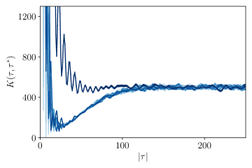
Figure S13: DSFF $K(\tau,\tau^{*})$ against $|\tau|$ at different values of $\theta$ from $0$ to $\pi/2$ in steps of $\pi/16$ (from light to dark blue) for the GinSE with the eigenvalues in the bottom half complex plane removed. We see that without the real eigenvalues, DSFF at $\theta=\pi/2$ after $|\tau|>\tau_{\mathrm{Hei}}$ saturates to the same plateau as DSFF at other angles, but the approach to the plateau is different (we suspect $\tau_{\mathrm{edge}}$ is large due to the disconnected DSFF of the modified spectra). Note that the matrix size $N=1024$ with sample size 2000.

Appendix F DSFF for $\theta$ near $0$ and $\pi/2$

As discussed in the previous section, the spectra of GinOE, QKT and CS contain complex conjugate pairs of eigenvalues and real eigenvalues, while the one of GinSE contain complex conjugate pairs only. These features lead to degeneracies in the set of eigenvalues projected along the axis defined by $\theta$, the “projected degeneracies” (c.f. interpretation of DSFF in the main text), which in turn make the DSFF behaviour special near $\theta=0,\pi/2$. Here we investigate the behaviour of DSFF near $\theta=0$ and $\theta=\pi/2$, firstly in the universality classes of GinOE (Fig. S14) and GinSE (Fig. S15), and secondly in the examples of QKT (Fig. S16) and CS (Fig. S17 and  S24). Note also that, to compare between the DSFF of non-RMT ensemble and DSFF of RMT, we have rescaled the width of the spectrum / the DOS in the complex plane of the non-RMT ensemble (see Appendix B and C) to unity, such that the transformed mean level spacing does not scale with matrix size $N$.

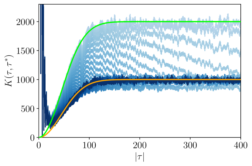
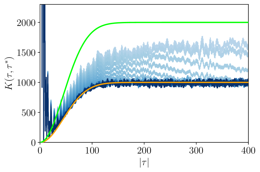
Figure S14: Left: DSFF $K(\tau,\tau^{*})$ of GinOE against $|\tau|$ from $\theta=0^{\circ}$ (light blue) to $\theta=2.64^{\circ}$ (dark blue) in steps of $0.24^{\circ}$. Right: DSFF $K(\tau,\tau^{*})$ of GinOE against $|\tau|$ from $\theta=86.48^{\circ}$ (dark blue) to $\theta=90^{\circ}$ (light blue) in steps of $0.32^{\circ}$. The orange (green) lines is (twice) the connected DSFF behaviour for GinUE (1st and 3rd terms in Eq. (3)). Note that the matrix size $N=1000$ with sample size 2000.

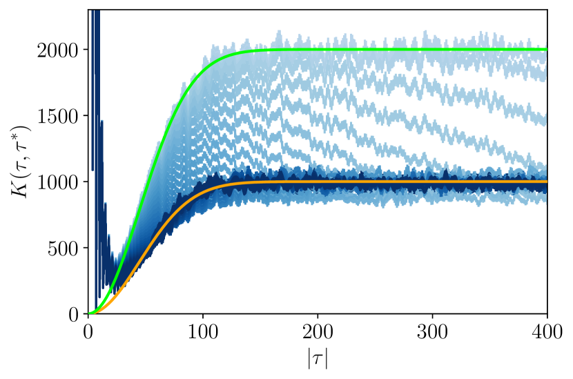
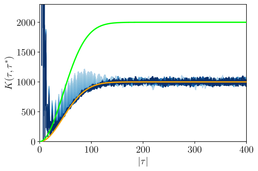
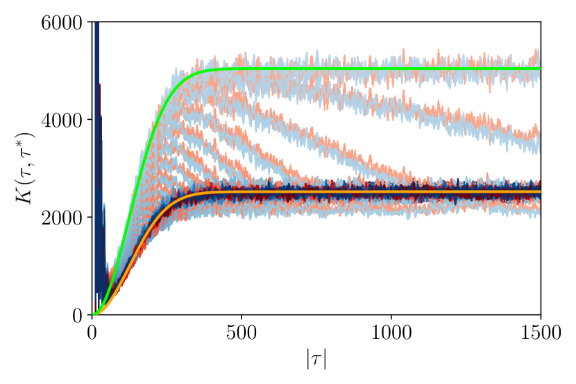
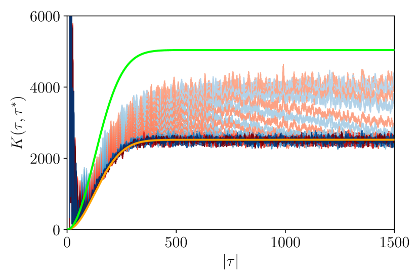
Figure S15: Left: DSFF $K(\tau,\tau^{*})$ of GinSE against $|\tau|$ from $\theta=0^{\circ}$ (light blue) to $\theta=2.64^{\circ}$ (dark blue) in steps of $0.24^{\circ}$. Right: DSFF $K(\tau,\tau^{*})$ of GinSE against $|\tau|$ from $\theta=86.48^{\circ}$ (dark blue) to $\theta=90^{\circ}$ (light blue) in steps of $0.32^{\circ}$. The orange (green) lines is (twice) the connected DSFF behaviour for GinUE (1st and 3rd terms in Eq. (3)). Note that the matrix size $N=1000$ with sample size 2000.

Figure S16: Left: DSFF $K(\tau,\tau^{*})$ of QKT with the kick with $j=35$ (blue) and DSFF of GinOE (red) against $|\tau|$ from $\theta=0^{\circ}$ (light) to $\theta=4^{\circ}$ (dark) in steps of $0.08^{\circ}$. Note that, as in the main text, the QKT with the kick is specified by Gaussianly-distributed $p\in\mathcal{N}(2,2/3)$ and $k_{0}\in\mathcal{N}(10,3)$. Right: DSFF $K(\tau,\tau^{*})$ of QKT (blue) with the same parameters and DSFF of GinOE (red) against $|\tau|$ from $\theta=87^{\circ}$ (light) to $\theta=90^{\circ}$ (dark) in steps of $0.06^{\circ}$. The orange (green) lines is (twice) the connected DSFF behaviour for GinUE (1st and 3rd terms in Eq. (3)). Note that the matrix size is $N=2521$ with sample size 2000.

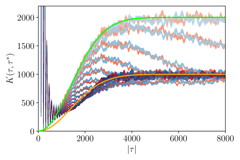
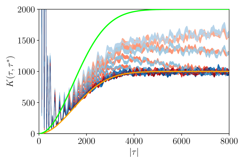
Figure S17: Left: DSFF $K(\tau,\tau^{*})$ of CS induced by CUE (blue) and DSFF of GinOE (red) against $|\tau|$ from $\theta=0^{\circ}$ (light) to $\theta=2.64^{\circ}$ (dark) in steps of $0.24^{\circ}$. Right: DSFF $K(\tau,\tau^{*})$ of CS induced by CUE (blue) and DSFF of GinOE (red) against $|\tau|$ from $\theta=86.48^{\circ}$ (light) to $\theta=90^{\circ}$ (dark) in steps of $0.32^{\circ}$. The orange (green) lines is (twice) the connected DSFF behaviour for GinUE (1st and 3rd terms in Eq. (3)). Note that the matrix size is $N=1000$ with sample size 2000.

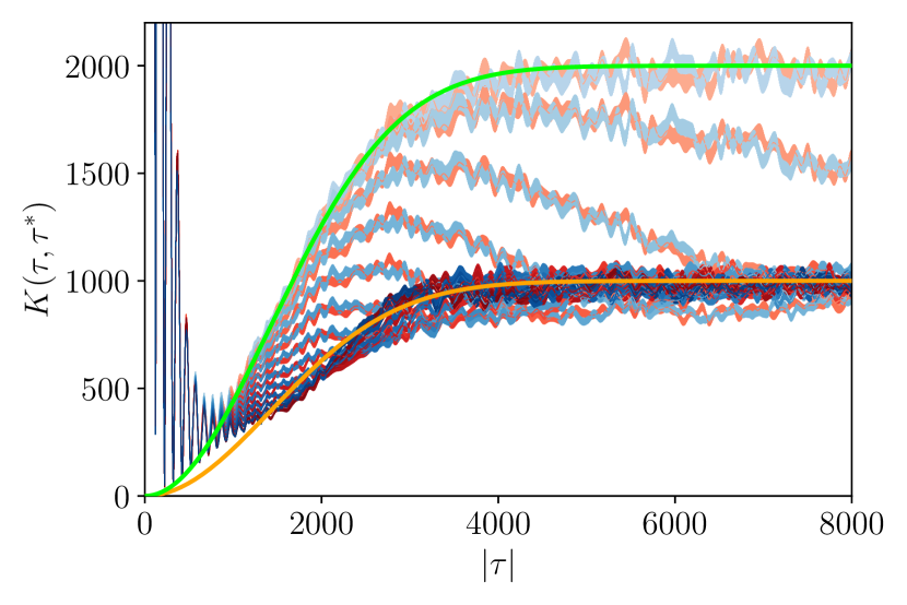
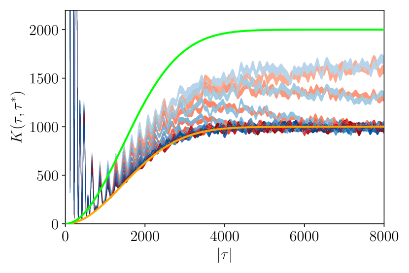
Figure S18: Left: DSFF $K(\tau,\tau^{*})$ of CS induced by GinUE (blue) and DSFF of GinOE (red) against $|\tau|$ from $\theta=0^{\circ}$ (light) to $\theta=2.64^{\circ}$ (dark) in steps of $0.24^{\circ}$. Right: DSFF $K(\tau,\tau^{*})$ of CS induced by CUE (blue) and DSFF of GinOE (red) against $|\tau|$ from $\theta=86.48^{\circ}$ (light) to $\theta=90^{\circ}$ (dark) in steps of $0.32^{\circ}$. The orange (green) lines is (twice) the connected DSFF behaviour for GinUE (1st and 3rd terms in Eq. (3)). Note that the matrix size is $N=1000$ with sample size 2000.

Appendix G Critical angle $\theta^{*}$

G.1 Definition of $\theta^{*}$

To investigate the deviation of DSFF near $\theta=0$ or $\theta=\pi/2$, we want to define a critical angle $\theta^{*}_{\phi}$ with $\phi=0,\pi/2$, such that for $K(|\tau|,{\theta^{*}_{0}}<\theta<\pi/2-{\theta^{*}_{\pi/2}})\approx K(|\tau|,\theta=\pi/4)$, i.e. the behaviour of DSFF along $\theta\in[{\theta^{*}_{0}},\pi/2-{\theta^{*}_{\pi/2}}]$ falls under the GinUE universality class. To this end, we first define an error function $\chi_{\phi}(\theta)\in[0,1]$,

$$\chi_{\phi}(\theta)=\frac{\sum_{|\tau|\leq{\tau_{\mathrm{Hei}}}}\Big{|}K(|\tau|,\theta)-K(|\tau|,\theta=\pi/4)\Big{|}^{2}}{\sum_{|\tau|\leq{\tau_{\mathrm{Hei}}}}\Big{|}K(|\tau|,\theta=\phi)-K(|\tau|,\theta=\pi/4)\Big{|}^{2}}\;,$$ (SG.1)

with $\phi=0$ or $\phi=\pi/2$. We have defined $\chi_{\phi}$ such that $\chi_{\phi}(\theta=\phi)=1$ and $\chi_{0}(\theta=\pi/4)=0$. To understand the typical behaviours of $\chi_{\phi}(\theta)$, we plot $\chi_{0}(\theta)$ for GinOE for $\theta\in[0,\pi/4]$ below.

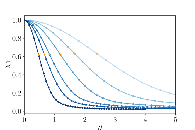
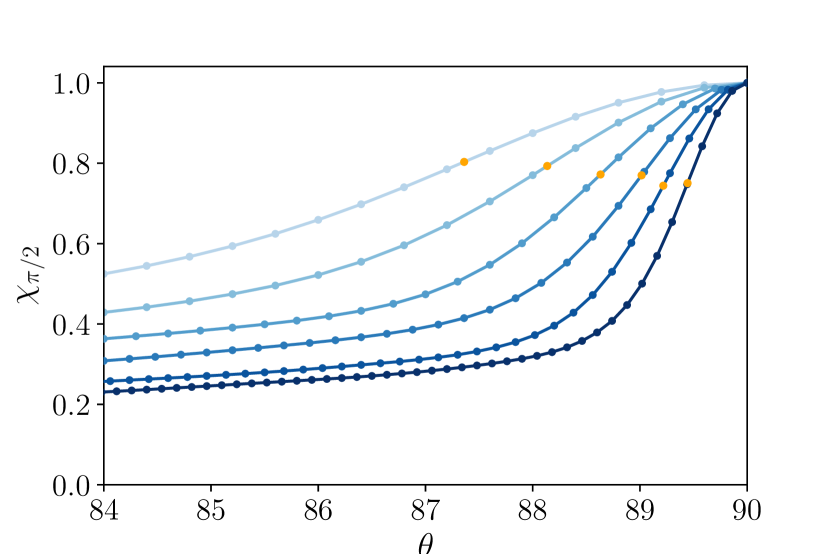
Figure S19: Left: $\chi_{0}(\theta)$ against $\theta$ for increasing matrix sizes from light blue to dark blue. Right: $\chi_{\pi/2}(\theta)$ against $\theta$ for increasing matrix sizes from light blue to dark blue. ${\theta^{*}_{\phi}}(N)$ is marked with orange dots. The matrix sizes are $N\in\{32,64,128,256,400,800\}$, and the sample size is 2000.

As a function of $\theta$, $\chi_{0}(\theta)$ first has a faster dip, then a slower decay. This shape is found in the DSFF of RMT, QKT (with the kick) and CS for multiple systems sizes. To define the critical angle $\theta^{*}_{\phi}$, we track the position of steepest point of the faster dip, by writing

$$\begin{split}\theta^{*}_{0}(N)&=\left\{\theta:\partial^{2}_{\theta}\chi_{\phi}(\theta)=0\right\}\\ \theta^{*}_{\pi/2}(N)&=\left\{\theta:\partial^{2}_{\theta}\chi_{\phi}(\pi/2-\theta)=0\right\}\end{split}\;,$$ (SG.2)

where $N$ is the size of the matrices in the ensemble of interest. Alternative definitions of $\theta^{*}_{\phi}$ that tracks the position of the faster dip in $\chi_{\phi}$ will give rise to similar scaling of $\theta^{*}_{\phi}$ in $N$ below.

G.2 Scaling of $\theta^{*}$

We compute ${\theta^{*}_{\phi}}$ for all ensembles discussed in the paper, and show that ${\theta^{*}_{\phi}}\approx\alpha N^{-1/2}$ for both $\phi=0$ and $\phi=\pi/2$. The one exception is the scaling of ${\theta^{*}_{\pi/2}}$ for GinSE, which is atypical because GinSE has no real eigenvalues, and thus no projected degeneracies at $\theta=\pi/2$ as discussed in the main text and in Appendix E. Nonetheless, there is deviation between DSFF at $\theta=\pi/2$ and the one at $\theta=\pi/4$ (see Appendix A). Note also that for CS induced by CUE and GinUE, $\partial^{2}_{\theta}\chi_{\pi/2}(\theta)$ shows a large amount fluctuation relative to the other ensembles (which we expect to go away if the sample sizes are increased). We instead use the definition, $\theta^{*}_{\pi/2}(N)=\max\left\{\theta:\chi_{\phi}(\pi/2-\theta)<\delta\right\}$.

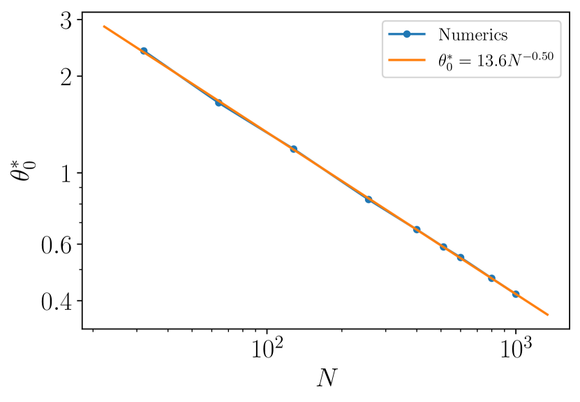
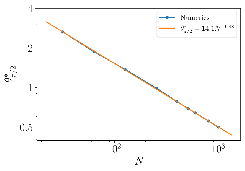
Figure S20: ${\theta^{*}_{0}}(N)$ (left) and ${\theta^{*}_{\pi/2}}(N)$ (right) of the GinOE for $N$ from $32$ to $1000$. The sample size is 2000.

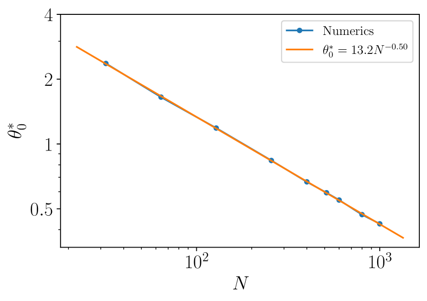
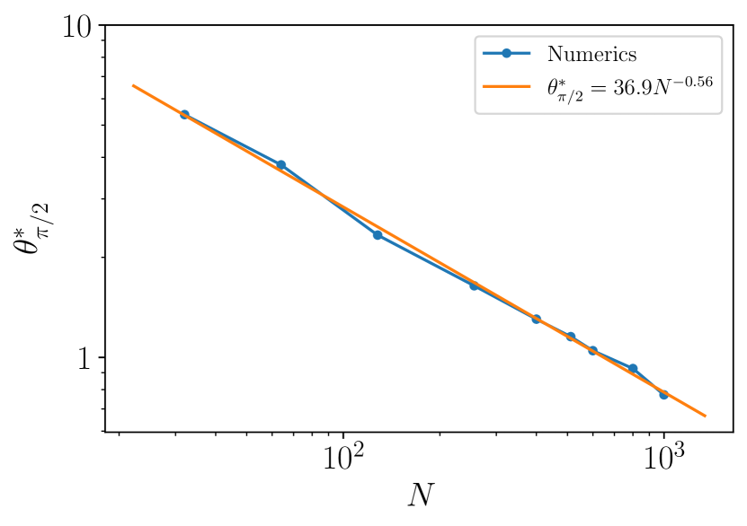
Figure S21: ${\theta^{*}_{0}}(N)$ (left) and ${\theta^{*}_{\pi/2}}(N)$ (right) of the GinSE for $N$ from $32$ to $1000$. The sample size is 2000.

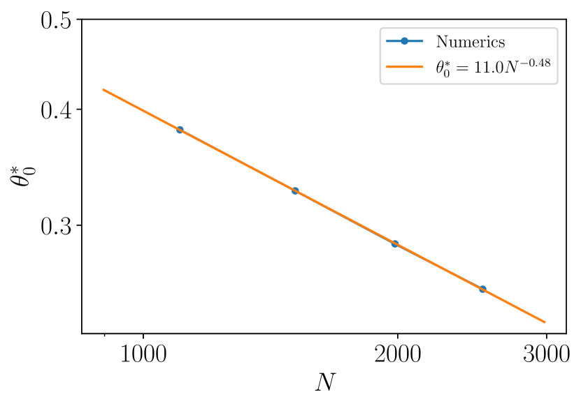
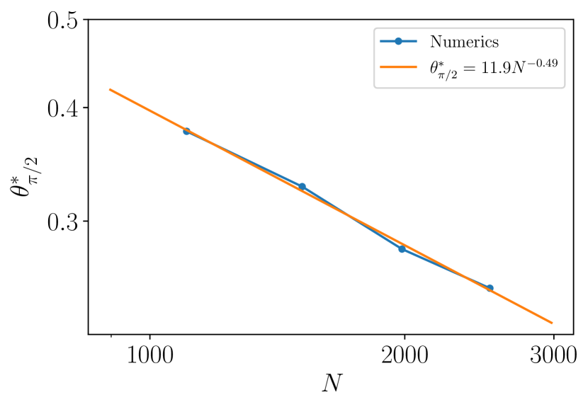
Figure S22: ${\theta^{*}_{0}}(N)$ (left) and ${\theta^{*}_{\pi/2}}(N)$ (right) of the QKT with the kick for $j=23,27,31$ and $35$, Gaussianly-distributed $p\in\mathcal{N}(2,2/3)$ and $k_{0}\in\mathcal{N}(10,3)$. The sample size is 2000.

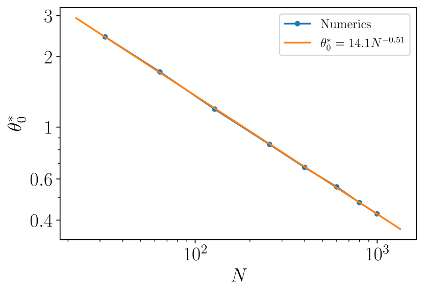
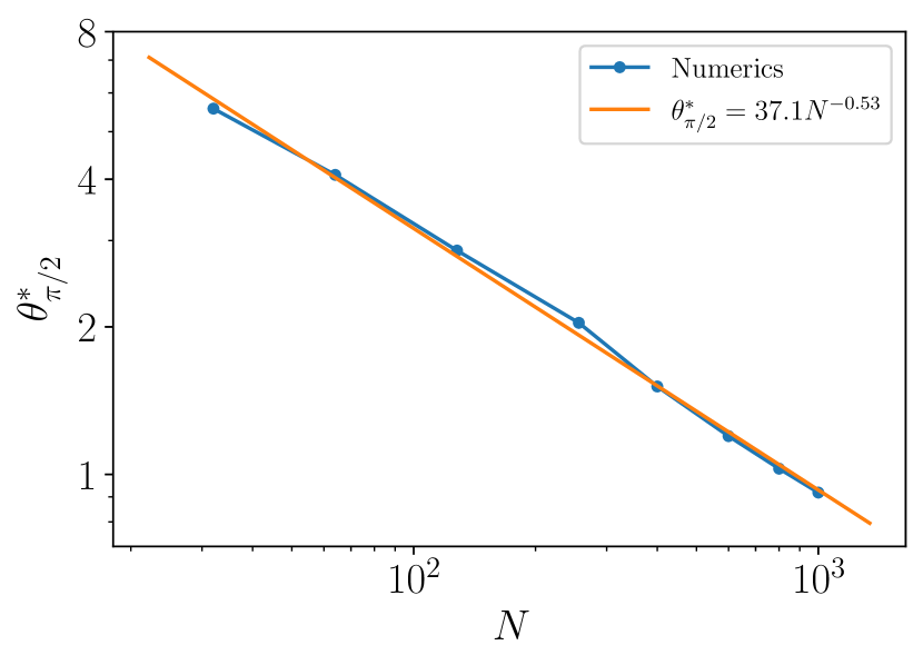
Figure S23: ${\theta^{*}_{0}}(N)$ (left) and ${\theta^{*}_{\pi/2}}(N)$ (right) of CS induced by CUE for $N$ from $32$ to $1000$. The sample size is 2000.

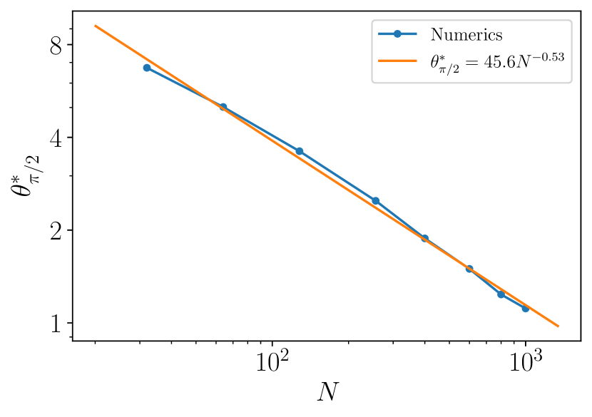
Figure S24: ${\theta^{*}_{0}}(N)$ (left) and ${\theta^{*}_{\pi/2}}(N)$ (right) of CS induced by GinUE for $N$ from $32$ to $1000$. The sample size is 2000.

G.3 Arguments for the scaling of $\theta^{*}$

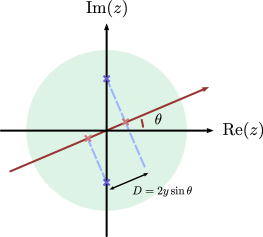
Figure S25: Illustration of the projected distance $D$ between a conjugate pair of eigenvalues $(z,z^{*})$ (blue) along an axis defined by $\theta$.

Here we provide an argument of why ${\theta^{*}_{\phi}}\propto N^{-1/2}$, where $N$ is the matrix size. Recall that DSFF $K(|\tau|,\theta)$ of a set of eigenvalues $\{z_{m}\}$ is equivalent to the SFF $K(|\tau|)$ of the same set of eigenvalues projected onto the axis defined by angle $\theta$. Let $(z,z^{*})$ be a pair of eigenvalues that are the complex conjugates of each other. Suppose $z=x+iy$ and $z^{*}=x-iy$ such that their distance in the complex plane is $2y$. The projected distance between $z$ and $z^{*}$ along a tilted axis defined by $\theta$ is $2y\sin\theta\approx 2y\theta$ for small $\theta$. Now suppose $(z,z^{*})$ are separated by the mean level spacing, i.e. $z=x+i\Delta/2$. The projected distance between $z$ and $z^{*}$ along the tilted axis is then $\theta\Delta$. Suppose that ${\tilde{\Delta}}=N^{-1}$ is the mean level spacing when $N$ eigenvalues are projected onto the $\theta$-axis. For $K(|\tau|,\theta>{\theta^{*}_{0}})\approx K(|\tau|,\theta=\pi/4)$ to be true, we must have $\theta\Delta>{\tilde{\Delta}}$, such that the late time plateau is not affected by the degeneracy along the $\theta$-axis. This gives a lower bound ${\theta^{*}_{\mathrm{LB}}}<{\theta^{*}_{\phi}}$, via

$$\begin{split}\Delta{\theta^{*}_{\mathrm{LB}}}&=O\left({\tilde{\Delta}}\right)\\ {\theta^{*}_{\mathrm{LB}}}&=O\left(\frac{1}{\sqrt{N}}\right)\;.\end{split}$$ (SG.3)

The numerics in Appendix G.2 suggests that this lower bound is being saturated.

References

- Mehta (2004) M. L. Mehta, Random Matrices (Academic Press, 2004).
- Bohigas et al. (1984) Oriol Bohigas, Marie-Joya Giannoni, and Charles Schmit, “Characterization of chaotic quantum spectra and universality of level fluctuation laws,” Physical Review Letters 52, 1 (1984).
- Berry and Tabor (1977) M. V. Berry and M. Tabor, “Level clustering in the regular spectrum,” Proceedings of the Royal Society of London. Series A, Mathematical and Physical Sciences 356, 375–394 (1977).
- Brody et al. (1981) T. A. Brody, J. Flores, J. B. French, P. A. Mello, A. Pandey, and S. S. M. Wong, “Random-matrix physics: spectrum and strength fluctuations,” Rev. Mod. Phys. 53, 385–479 (1981).
- Beenakker (1997) C. W. J. Beenakker, “Random-matrix theory of quantum transport,” Rev. Mod. Phys. 69, 731–808 (1997).
- Beenakker (2015) C. W. J. Beenakker, “Random-matrix theory of majorana fermions and topological superconductors,” Rev. Mod. Phys. 87, 1037–1066 (2015).
- D’Alessio et al. (2016) Luca D’Alessio, Yariv Kafri, Anatoli Polkovnikov, and Marcos Rigol, “From quantum chaos and eigenstate thermalization to statistical mechanics and thermodynamics,” Advances in Physics 65, 239–362 (2016).
- García-García and Verbaarschot (2016) Antonio M. García-García and Jacobus J. M. Verbaarschot, “Spectral and thermodynamic properties of the sachdev-ye-kitaev model,” Phys. Rev. D 94, 126010 (2016).
- Cotler et al. (2017a) Jordan S. Cotler, Guy Gur-Ari, Masanori Hanada, Joseph Polchinski, Phil Saad, Stephen H. Shenker, Douglas Stanford, Alexandre Streicher, and Masaki Tezuka, “Black holes and random matrices,” Journal of High Energy Physics 2017 (2017a), 10.1007/jhep05(2017)118.
- Cotler et al. (2017b) Jordan Cotler, Nicholas Hunter-Jones, Junyu Liu, and Beni Yoshida, “Chaos, complexity, and random matrices,” Journal of High Energy Physics 2017, 48 (2017b).
- Smilga (1995) A V Smilga, Continuous Advances in QCD (WORLD SCIENTIFIC, 1995) https://www.worldscientific.com/doi/pdf/10.1142/2435 .
- Akemann (2018) Gernot Akemann, “Random matrix theory and quantum chromodynamics,” Oxford Scholarship Online (2018), 10.1093/oso/9780198797319.003.0005.
- Schroeder (2008) Manfred Schroeder, Number Theory in Science and Communication: With Applications in Cryptography, Physics, Digital Information, Computing, and Self-Similarity, 5th ed. (Springer Publishing Company, Incorporated, 2008).
- Tulino and Verdú (2004) Antonia M. Tulino and Sergio Verdú, “Random matrix theory and wireless communications,” Foundations and Trends® in Communications and Information Theory 1, 1–182 (2004).
- Feng et al. (2017) Liang Feng, Ramy El-Ganainy, and Li Ge, “Non-hermitian photonics based on parity–time symmetry,” Nature Photonics 11, 752–762 (2017).
- Carmichael (1993) Howard Carmichael, “An Open Systems Approach to Quantum Optics,” Lecture Notes in Physics Monographs 18 (1993), 10.1007/978-3-540-47620-7.
- El-Ganainy et al. (2018) Ramy El-Ganainy, Konstantinos G. Makris, Mercedeh Khajavikhan, Ziad H. Musslimani, Stefan Rotter, and Demetrios N. Christodoulides, “Non-hermitian physics and pt symmetry,” Nature Physics 14, 11–19 (2018).
- Ma and Sheng (2016) Guancong Ma and Ping Sheng, “Acoustic metamaterials: From local resonances to broad horizons,” Science Advances 2 (2016), 10.1126/sciadv.1501595, https://advances.sciencemag.org/content/2/2/e1501595.full.pdf .
- Cummer et al. (2016) Steven A. Cummer, Johan Christensen, and Andrea Alù, “Controlling sound with acoustic metamaterials,” Nature Reviews Materials 1, 16001 (2016).
- Bender (2007) Carl M Bender, “Making sense of non-hermitian hamiltonians,” Reports on Progress in Physics 70, 947–1018 (2007).
- Özdemir et al. (2019) Ş K. Özdemir, S. Rotter, F. Nori, and L. Yang, “Parity–time symmetry and exceptional points in photonics,” Nature Materials 18, 783–798 (2019).
- Moiseyev (1998) Nimrod Moiseyev, “Quantum theory of resonances: calculating energies, widths and cross-sections by complex scaling,” Physics Reports 302, 212 – 293 (1998).
- Muga et al. (2004) J. G. Muga, J. P. Palao, B. Navarro, and I. L. Egusquiza, “Complex absorbing potentials,” Physics Reports 395, 357–426 (2004).
- Cao and Wiersig (2015) Hui Cao and Jan Wiersig, “Dielectric microcavities: Model systems for wave chaos and non-hermitian physics,” Rev. Mod. Phys. 87, 61–111 (2015).
- Rotter and Gigan (2017) Stefan Rotter and Sylvain Gigan, “Light fields in complex media: Mesoscopic scattering meets wave control,” Rev. Mod. Phys. 89, 015005 (2017).
- Daley (2014) Andrew J. Daley, “Quantum trajectories and open many-body quantum systems,” Advances in Physics 63, 77–149 (2014).
- Kuhr (2016) Stefan Kuhr, “Quantum-gas microscopes: a new tool for cold-atom quantum simulators,” National Science Review 3, 170–172 (2016), https://academic.oup.com/nsr/article-pdf/3/2/170/31565423/nww023.pdf .
- Deng et al. (2010) Hui Deng, Hartmut Haug, and Yoshihisa Yamamoto, “Exciton-polariton bose-einstein condensation,” Rev. Mod. Phys. 82, 1489–1537 (2010).
- Müller et al. (2012) M. Müller, S. Diehl, G. Pupillo, and P. Zoller, “Engineered open systems and quantum simulations with atoms and ions,” (2012), arXiv:1203.6595 [quant-ph] .
- Ritsch et al. (2013) Helmut Ritsch, Peter Domokos, Ferdinand Brennecke, and Tilman Esslinger, “Cold atoms in cavity-generated dynamical optical potentials,” Rev. Mod. Phys. 85, 553–601 (2013).
- Sieberer et al. (2016) L M Sieberer, M Buchhold, and S Diehl, “Keldysh field theory for driven open quantum systems,” Reports on Progress in Physics 79, 096001 (2016).
- Chou et al. (2011) T Chou, K Mallick, and R K P Zia, “Non-equilibrium statistical mechanics: from a paradigmatic model to biological transport,” Reports on Progress in Physics 74, 116601 (2011).
- Marchetti et al. (2013) M. C. Marchetti, J. F. Joanny, S. Ramaswamy, T. B. Liverpool, J. Prost, Madan Rao, and R. Aditi Simha, “Hydrodynamics of soft active matter,” Rev. Mod. Phys. 85, 1143–1189 (2013).
- Akemann et al. (2019) Gernot Akemann, Mario Kieburg, Adam Mielke, and Toma ž Prosen, “Universal signature from integrability to chaos in dissipative open quantum systems,” Phys. Rev. Lett. 123, 254101 (2019).
- Can (2019) Tankut Can, “Random lindblad dynamics,” Journal of Physics A: Mathematical and Theoretical 52, 485302 (2019).
- Can et al. (2019) Tankut Can, Vadim Oganesyan, Dror Orgad, and Sarang Gopalakrishnan, “Spectral gaps and midgap states in random quantum master equations,” Phys. Rev. Lett. 123, 234103 (2019).
- Sá et al. (2019a) Lucas Sá, Pedro Ribeiro, and Tomaž Prosen, “Complex spacing ratios: a signature of dissipative quantum chaos,” arXiv e-prints , arXiv:1910.12784 (2019a), arXiv:1910.12784 [cond-mat.stat-mech] .
- Sá et al. (2019b) Lucas Sá, Pedro Ribeiro, and Tomaž Prosen, “Spectral and Steady-State Properties of Random Liouvillians,” arXiv e-prints , arXiv:1905.02155 (2019b), arXiv:1905.02155 [quant-ph] .
- Sá et al. (2020) Lucas Sá, Pedro Ribeiro, Tankut Can, and Toma ž Prosen, “Spectral transitions and universal steady states in random kraus maps and circuits,” Phys. Rev. B 102, 134310 (2020).
- Sá et al. (2020) Lucas Sá, Pedro Ribeiro, and Tomaž Prosen, “Integrable non-unitary open quantum circuits,” (2020), arXiv:2011.06565 [cond-mat.stat-mech] .
- Álvaro Rubio-García et al. (2021) Álvaro Rubio-García, Rafael A. Molina, and Jorge Dukelsky, “From integrability to chaos in quantum liouvillians,” (2021), arXiv:2102.13452 [nlin.CD] .
- Wang et al. (2020) Kevin Wang, Francesco Piazza, and David J. Luitz, “Hierarchy of relaxation timescales in local random liouvillians,” Phys. Rev. Lett. 124, 100604 (2020).
- Denisov et al. (2019) Sergey Denisov, Tetyana Laptyeva, Wojciech Tarnowski, Dariusz Chruściński, and Karol Życzkowski, “Universal spectra of random lindblad operators,” Physical Review Letters 123 (2019), 10.1103/physrevlett.123.140403.
- Huang and Shklovskii (2020) Yi Huang and B. I. Shklovskii, “Anderson transition in three-dimensional systems with non-hermitian disorder,” Phys. Rev. B 101, 014204 (2020).
- Hamazaki et al. (2019) Ryusuke Hamazaki, Kohei Kawabata, and Masahito Ueda, “Non-hermitian many-body localization,” Phys. Rev. Lett. 123, 090603 (2019).
- Tzortzakakis et al. (2020) A. F. Tzortzakakis, K. G. Makris, and E. N. Economou, “Non-hermitian disorder in two-dimensional optical lattices,” Phys. Rev. B 101, 014202 (2020).
- Peron et al. (2020) Thomas Peron, Bruno Messias F. de Resende, Francisco A. Rodrigues, Luciano da F. Costa, and J. A. Méndez-Bermúdez, “Spacing ratio characterization of the spectra of directed random networks,” Phys. Rev. E 102, 062305 (2020).
- Borgonovi et al. (1991) F. Borgonovi, I. Guarneri, and D. L. Shepelyansky, “Statistics of quantum lifetimes in a classically chaotic system,” Phys. Rev. A 43, 4517–4520 (1991).
- (49) Jiachen Li, Tomaž Prosen, and Amos Chan, in preparation .
- Haake (2010) F. Haake, Quantum Signatures of Chaos (Springer, 2010).
- Note (1) SFF involves only two sums over eigenlevels as supposed to four sums in observables like the out-of-time-order correlator or the quantum purity. Note also that the finer correlations between eigenlevels can be captured by the so-called higher-point SFFCotler et al. (2017b); Liu (2018).
- Kos et al. (2018) Pavel Kos, Marko Ljubotina, and Toma ž Prosen, “Many-body quantum chaos: Analytic connection to random matrix theory,” Phys. Rev. X 8, 021062 (2018).
- Bertini et al. (2018) Bruno Bertini, Pavel Kos, and Tomaž Prosen, “Exact spectral form factor in a minimal model of many-body quantum chaos,” Physical review letters 121, 264101 (2018).
- Roy and Prosen (2020) Dibyendu Roy and Tomaž Prosen, “Random matrix spectral form factor in kicked interacting fermionic chains,” (2020), arXiv:2005.10489 [cond-mat.stat-mech] .
- Flack et al. (2020) Ana Flack, Bruno Bertini, and Tomaz Prosen, “Statistics of the spectral form factor in the self-dual kicked ising model,” (2020), arXiv:2009.03199 [nlin.CD] .
- Chan et al. (2018a) Amos Chan, Andrea De Luca, and J. T. Chalker, “Solution of a minimal model for many-body quantum chaos,” Phys. Rev. X 8, 041019 (2018a).
- Chan et al. (2018b) Amos Chan, Andrea De Luca, and J. T. Chalker, “Spectral statistics in spatially extended chaotic quantum many-body systems,” Phys. Rev. Lett. 121, 060601 (2018b).
- Friedman et al. (2019) Aaron J. Friedman, Amos Chan, Andrea De Luca, and J. T. Chalker, “Spectral statistics and many-body quantum chaos with conserved charge,” Phys. Rev. Lett. 123, 210603 (2019).
- Moudgalya et al. (2020) Sanjay Moudgalya, Abhinav Prem, David A. Huse, and Amos Chan, “Spectral statistics in constrained many-body quantum chaotic systems,” (2020), arXiv:2009.11863 [cond-mat.stat-mech] .
- Garratt and Chalker (2020) S. J. Garratt and J. T. Chalker, “Many-body quantum chaos and the local pairing of feynman histories,” (2020), arXiv:2008.01697 [cond-mat.stat-mech] .
- Gharibyan et al. (2018) Hrant Gharibyan, Masanori Hanada, Stephen H. Shenker, and Masaki Tezuka, “Onset of random matrix behavior in scrambling systems,” Journal of High Energy Physics 2018 (2018), 10.1007/jhep07(2018)124.
- Chan et al. (2020) Amos Chan, Andrea De Luca, and J. T. Chalker, “Spectral lyapunov exponents in chaotic and localized many-body quantum systems,” (2020), arXiv:2012.05295 [cond-mat.stat-mech] .
- Chan et al. (2021) Amos Chan, Saumya Shivam, David A. Huse, and Andrea De Luca, “Many-body quantum chaos and space-time translational invariance,” (2021), arXiv:2109.04475 [cond-mat.stat-mech] .
- Saad et al. (2019) Phil Saad, Stephen H. Shenker, and Douglas Stanford, “A semiclassical ramp in syk and in gravity,” (2019), arXiv:1806.06840 [hep-th] .
- Bertini et al. (2021) Bruno Bertini, Pavel Kos, and Tomaz Prosen, “Random matrix spectral form factor of dual-unitary quantum circuits,” (2021), arXiv:2012.12254 [math-ph] .
- Winer and Swingle (2020) Michael Winer and Brian Swingle, “Hydrodynamic theory of the connected spectral form factor,” (2020), arXiv:2012.01436 [cond-mat.stat-mech] .
- Šuntajs et al. (2020) Jan Šuntajs, Janez Bonča, Tomaž Prosen, and Lev Vidmar, “Quantum chaos challenges many-body localization,” Physical Review E 102 (2020), 10.1103/physreve.102.062144.
- Ginibre (1965) Jean Ginibre, “Statistical ensembles of complex, quaternion, and real matrices,” Journal of Mathematical Physics 6, 440–449 (1965), https://doi.org/10.1063/1.1704292 .
- (69) See supplementary material at [url] for DSFF of additional ensembles (with modified spectra), discussion of DSFF near and , analysis on critical angles , details about DOS, and the scaling of .
- Baus and Hansen (1980) Marc Baus and Jean-Pierre Hansen, “Statistical mechanics of simple coulomb systems,” Physics Reports 59, 1–94 (1980).
- Torquato and Stillinger (2003) Salvatore Torquato and Frank H. Stillinger, “Local density fluctuations, hyperuniformity, and order metrics,” Phys. Rev. E 68, 041113 (2003).
- Torquato (2018) Salvatore Torquato, “Hyperuniform states of matter,” Physics Reports 745, 1–95 (2018).
- Lehmann and Sommers (1991) Nils Lehmann and Hans-Jürgen Sommers, “Eigenvalue statistics of random real matrices,” Phys. Rev. Lett. 67, 2403–2403 (1991).
- Forrester and Nagao (2007) Peter J. Forrester and Taro Nagao, “Eigenvalue statistics of the real ginibre ensemble,” Phys. Rev. Lett. 99, 050603 (2007).
- Borodin and Sinclair (2009) A. Borodin and C. D. Sinclair, “The ginibre ensemble of real random matrices and its scaling limits,” Communications in Mathematical Physics 291, 177–224 (2009).
- Akemann and Kanzieper (2007) Gernot Akemann and Eugene Kanzieper, “Integrable structure of ginibre’s ensemble of real random matrices and a pfaffian integration theorem,” Journal of Statistical Physics 129, 1159–1231 (2007).
- Sommers and Wieczorek (2008) Hans-Jürgen Sommers and Waldemar Wieczorek, “General eigenvalue correlations for the real ginibre ensemble,” Journal of Physics A: Mathematical and Theoretical 41, 405003 (2008).
- Grobe et al. (1988) Rainer Grobe, Fritz Haake, and Hans-Jürgen Sommers, “Quantum distinction of regular and chaotic dissipative motion,” Phys. Rev. Lett. 61, 1899–1902 (1988).
- Haake et al. (1987) F. Haake, M. Kuś, and R. Scharf, “Classical and quantum chaos for a kicked top,” Zeitschrift für Physik B Condensed Matter 65, 381–395 (1987).
- Gorin et al. (2006) Thomas Gorin, Tomaž Prosen, Thomas H. Seligman, and Marko Žnidarič, “Dynamics of loschmidt echoes and fidelity decay,” Physics Reports 435, 33–156 (2006).
- Smith et al. (2004) Greg A. Smith, Souma Chaudhury, Andrew Silberfarb, Ivan H. Deutsch, and Poul S. Jessen, “Continuous weak measurement and nonlinear dynamics in a cold spin ensemble,” Phys. Rev. Lett. 93, 163602 (2004).
- Nielsen and Chuang (2010) Michael A. Nielsen and Isaac L. Chuang, Quantum Computation and Quantum Information: 10th Anniversary Edition (Cambridge University Press, 2010).
- Tanner (2001) Gregor Tanner, “Unitary-stochastic matrix ensembles and spectral statistics,” Journal of Physics A: Mathematical and General 34, 8485–8500 (2001).
- Tanner (2000) Gregor Tanner, “Spectral statistics for unitary transfer matrices of binary graphs,” Journal of Physics A: Mathematical and General 33, 3567–3585 (2000).
- Gnutzmann and Smilansky (2006) Sven Gnutzmann and Uzy Smilansky, “Quantum graphs: Applications to quantum chaos and universal spectral statistics,” Advances in Physics 55, 527–625 (2006), https://doi.org/10.1080/00018730600908042 .
- Marshall et al. (2011) Albert W. Marshall, Ingram Olkin, and Barry C. Arnold, Inequalities: Theory of Majorization and its Applications, 2nd ed., Vol. 143 (Springer, 2011).
- Nielsen (1999) M. A. Nielsen, “Conditions for a class of entanglement transformations,” Phys. Rev. Lett. 83, 436–439 (1999).
- Nielsen (2000) M. A. Nielsen, “Probability distributions consistent with a mixed state,” Phys. Rev. A 62, 052308 (2000).
- Hammerer et al. (2002) K. Hammerer, G. Vidal, and J. I. Cirac, “Characterization of nonlocal gates,” Phys. Rev. A 66, 062321 (2002).
- Zyczkowski et al. (2003) Karol Zyczkowski, Marek Kus, Wojciech S omczy ski, and Hans-J rgen Sommers, “Random unistochastic matrices,” Journal of Physics A: Mathematical and General 36, 3425–3450 (2003).
- Magnea (2008) Ulrika Magnea, “Random matrices beyond the cartan classification,” Journal of Physics A: Mathematical and Theoretical 41, 045203 (2008).
- Kawabata et al. (2019) Kohei Kawabata, Ken Shiozaki, Masahito Ueda, and Masatoshi Sato, “Symmetry and topology in non-hermitian physics,” Phys. Rev. X 9, 041015 (2019).
- Bernard and LeClair (2002) Denis Bernard and André LeClair, “A classification of non-hermitian random matrices,” in Statistical Field Theories, edited by Andrea Cappelli and Giuseppe Mussardo (Springer Netherlands, Dordrecht, 2002) pp. 207–214.
- Hamazaki et al. (2020) Ryusuke Hamazaki, Kohei Kawabata, Naoto Kura, and Masahito Ueda, “Universality classes of non-hermitian random matrices,” Physical Review Research 2 (2020), 10.1103/physrevresearch.2.023286.
- Skinner et al. (2019) Brian Skinner, Jonathan Ruhman, and Adam Nahum, “Measurement-induced phase transitions in the dynamics of entanglement,” Physical Review X 9 (2019), 10.1103/physrevx.9.031009.
- Li et al. (2018) Yaodong Li, Xiao Chen, and Matthew P. A. Fisher, “Quantum zeno effect and the many-body entanglement transition,” Physical Review B 98 (2018), 10.1103/physrevb.98.205136.
- Li et al. (2019) Yaodong Li, Xiao Chen, and Matthew P. A. Fisher, “Measurement-driven entanglement transition in hybrid quantum circuits,” Physical Review B 100 (2019), 10.1103/physrevb.100.134306.
- Chan et al. (2019) Amos Chan, Rahul M. Nandkishore, Michael Pretko, and Graeme Smith, “Unitary-projective entanglement dynamics,” Phys. Rev. B 99, 224307 (2019).
- Bao et al. (2020) Yimu Bao, Soonwon Choi, and Ehud Altman, “Theory of the phase transition in random unitary circuits with measurements,” Phys. Rev. B 101, 104301 (2020).
- Jian et al. (2020) Chao-Ming Jian, Yi-Zhuang You, Romain Vasseur, and Andreas W. W. Ludwig, “Measurement-induced criticality in random quantum circuits,” Physical Review B 101 (2020), 10.1103/physrevb.101.104302.
- Zabalo et al. (2020) Aidan Zabalo, Michael J. Gullans, Justin H. Wilson, Sarang Gopalakrishnan, David A. Huse, and J. H. Pixley, “Critical properties of the measurement-induced transition in random quantum circuits,” Physical Review B 101 (2020), 10.1103/physrevb.101.060301.
- Liu (2018) Junyu Liu, “Spectral form factors and late time quantum chaos,” Phys. Rev. D 98, 086026 (2018).