Hardware error correction for programmable photonics

Abstract

Programmable photonic circuits of reconfigurable interferometers can be used to implement arbitrary operations on optical modes, facilitating a flexible platform for accelerating tasks in quantum simulation, signal processing, and artificial intelligence. A major obstacle to scaling up these systems is static fabrication error, where small component errors within each device accrue to produce significant errors within the circuit computation. Mitigating this error usually requires numerical optimization dependent on real-time feedback from the circuit, which can greatly limit the scalability of the hardware. Here we present a deterministic approach to correcting circuit errors by locally correcting hardware errors within individual optical gates. We apply our approach to simulations of large scale optical neural networks and infinite impulse response filters implemented in programmable photonics, finding that they remain resilient to component error well beyond modern day process tolerances. Our results highlight a new avenue for scaling up programmable photonics to hundreds of modes within current day fabrication processes.

1 Introduction

Integrated photonics is a key technology for optical communications and is advancing rapidly for applications in sensing, metrology, signal processing, and computation. Programmable photonic circuits of optical interferometers, which can implement arbitrary filters and passively compute matrix operations on optical modes, are the optical analogue to field programmable gate arrays (FPGAs) and enable photonic circuits to be flexibly reconfigured post-fabrication by software [1, 2]. Experimental demonstrations of these circuits have already shown working systems operating on up to tens of optical modes, which have been used to accelerate tasks in quantum simulation [3, 4, 5, 6, 7], mode unscrambling [8, 9, 10, 11, 12], signal processing [13, 14], combinatorial optimization [15], and artificial intelligence [16].

While scaling up these systems to hundreds or thousands of modes would be immensely beneficial, doing so will require precise fabrication of tens of thousands of optical interferometers. Unfortunately, static component errors induced by process variation introduce errors that rapidly accrue for larger systems, limiting their usefulness for many applications. This is because the decomposition [17, 18] and optimization techniques used to program these circuits assume that all of the components are ideal; thus, any component errors result in a programming of the wrong operation. Component imprecision therefore has serious implications for the future of these systems; for example, beamsplitter variation as small as 2%, which is a typical wafer-level variance [19], has been shown to degrade accuracy by nearly 50% for feedforward circuits used to implement classifiers for the MNIST image recognition task [20]. Alternative programmable architectures, such as recirculating waveguide meshes consisting of triangular or hexagonal MZI lattices [21, 22, 13], are similarly susceptible to component-induced error; device variation within these circuits introduces errors that will alter the response of phase-sensitive filters [23]. These systems’ degree of sensitivity to component variation makes their control challenging when scaling up to large numbers of modes.

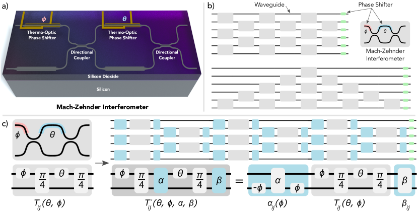
Figure 1: a) A Mach-Zehnder interferometer (MZI) on the silicon-on-insulator platform is composed of two 50-50 splitters, implemented with directional couplers, and an external phase shifter $\phi$ and internal phase shifter $\theta$ implemented with thermo-optic phase shifters. These devices act as electrically-controlled $2\times 2$ optical gates in programmable photonics. b) Arbitrary higher-dimensional matrix operations can be implemented by connecting $N(N-1)/2$ MZIs in a rectangular (top) or triangular (bottom) configuration. The Reck (triangular) and Clements (rectangular) decompositions [17, 18] describe a procedure for computing the phase settings for each MZI, but they assume the components are ideal. c) A realistic MZI implemented on a photonics platform will have splitting errors $\alpha,\beta$ for the two directional couplers within the interferometer. The effect of these hardware errors is to left- and right-multiply each programmable $2\times 2$ unitary $T_{ij}(\theta,\phi)$ implemented by an MZI by error matrices $\beta_{ij},\alpha_{ij}(\phi)$. Applying the standard decomposition for ideal components to these imperfect optical gates will not produce the correct gate operation.

Hardware errors are usually compensated for with numerical optimization. A number of global optimization approaches have been proposed in the past, including nonlinear optimization [24, 25, 26, 27, 28], gradient descent [29], and in-situ backpropagation and training for neural networks [30]. These strategies, however, are time-consuming and can scale poorly with circuit size. Moreover, it is often inefficient to retrain hardware settings for each individual chip. For many tasks, such as machine learning, model training is energy intensive; if the same model parameters are broadcast to thousands of chips within a data center, retraining the model for each chip with a unique set of component imprecisions will be very costly. One can instead employ progressive algorithms making use of local feedback [31, 32]; however, these algorithms, which iteratively optimize the settings of one device at a time, require $O(N^{2})$ tap photodiodes to monitor the optical power within each individual interferometer. This requirement greatly increases the number of electrical lines and overall power consumption of the system.

This focus on in-situ approaches reveals a critical roadblock for programmable photonics compared to electronic FPGAs. An FPGA does not optimize hardware settings in real time off readings taken directly from the chip; rather, control software takes it for granted that the logic gates are ideal and maps the requested function into a netlist that can be placed and routed within the chip. A similar capability for programmable photonics would greatly improve the scalability of these systems; if this were the case, a desired optical function could be trained once on an idealized software model and ported over to many chips. The challenge for programmable photonics is that unlike FPGAs, photonic circuits are analog systems that are far more sensitive to errors within individual components. Enabling this level of scalability will therefore require the ability to deterministically correct hardware errors in photonic chips.

If a unitary operation is realizable by an imperfect photonic circuit, it should not require optimization to deduce the required settings; rather, a small perturbation in the device behavior due to component deviation should translate directly to a small perturbation in the interferometer’s phase settings to recover the original unitary. This insight has led us to consider a local approach that corrects hardware errors one at a time within each optical gate composing the circuit. In this article, we present an approach to directly correct hardware errors for a programmable photonic circuit. Our algorithm outperforms previous approaches in several key respects: 1) it is flexible, requiring only a one time device calibration to directly compute the hardware settings for any given unitary; 2) for sufficiently low hardware errors the computed settings yield the exact unitary desired; and 3) our approach requires minimal overhead and does not make use of additional interferometers or internal detectors within every device. Our analysis is focused on feedforward programmable circuits that implement arbitrary unitary matrices, as these systems have the most demanding requirements for fabrication precision. However, our approach is a local error correction strategy that individually corrects each $2\times 2$ optical gate within the circuit. It therefore does not assume any particular structure to the circuit and can be generalized to any programmable architecture making use of interferometers, including feedforward circuits with redundant devices and recirculating waveguide meshes.

2 Hardware Error Correction

Local error correction requires characterization of each phase shifter and passive splitter in the photonic circuit. The calibration is performed once with the results stored in a lookup table; any arbitrary function can then be programmed by computing the settings for an ideal set of MZIs and converting them, one by one, to the corresponding settings for an imperfect device. In the Supplementary Information (Sec. I.), we describe how to calibrate these parameters using detectors only at the circuit outputs; assuming these errors are known, we can proceed with error correction as follows.

The fundamental optical gate of a programmable photonic circuit is a $2\times 2$ Mach-Zehnder interferometer (MZI) composed of an external phase shifter on one input, two 50-50 beamsplitters, and an internal phase shifter on one of the modes between the splitters (Fig. 1a). This device is an electrically programmable beamsplitter capable of performing a $2\times 2$ unitary operation $T_{ij}(\theta,\phi)$ on optical modes $i,j$ parameterized by the external phase shift $\phi$ and the internal phase shift $\theta$.

On an integrated photonics platform, the 50-50 splitters can be realized by a directional coupler or multimode interferometer (MMI); the operation of these splitters can be described by a $2\times 2$ matrix:

$$\begin{bmatrix}\cos(\pi/4+\alpha)&i\sin(\pi/4+\alpha)\\ i\sin(\pi/4+\alpha)&\cos(\pi/4+\alpha)\end{bmatrix}$$ (1)

where $\alpha$ describes the deviation from an ideal 50-50 splitting behavior. For an ideal splitter $\alpha=0$, this matrix reduces to:

$$\frac{1}{\sqrt{2}}\begin{bmatrix}1&i\\ i&1\end{bmatrix}$$ (2)

The overall operation $T_{ij}(\theta,\phi)$ performed by a single ideal MZI is therefore:

$$T_{ij}(\theta,\phi) =\frac{1}{2}\begin{bmatrix}1&i\\ i&1\end{bmatrix}\begin{bmatrix}e^{i\theta}&0\\ 0&1\end{bmatrix}\begin{bmatrix}1&i\\ i&1\end{bmatrix}\begin{bmatrix}e^{i\phi}&0\\ 0&1\end{bmatrix}$$

$$=ie^{i\theta/2}\begin{bmatrix}e^{i\phi}\sin(\theta/2)&\cos(\theta/2)\\ e^{i\phi}\cos(\theta/2)&-\sin(\theta/2)\end{bmatrix}$$ (3)

where $\theta,\phi$ are single-mode phase shifts on the top arm.

Higher dimensional matrix operations can be implemented with this unit cell by applying the Clements [18] and Reck [17] decompositions (Fig. 1b). These algorithms decompose an arbitrary $N$-dimensional unitary $U$ into a product of $N(N-1)/2$ two-dimensional unitaries computed by interference between nearest-neighbor optical modes, followed by phase shifts on the output modes corresponding to a diagonal matrix $D$:

$$U=D\prod T_{ij}(\theta,\phi)$$ (4)

We now analyze the impact of fabrication error. If the MZI has imperfect splitters with errors $\alpha,\beta$, the operation of the MZI must now be parameterized with four variables $T^{\prime}_{ij}(\theta,\phi,\alpha,\beta)$ (Fig. 1c):

$$ie^{i\theta/2} \begin{bmatrix}[2.5]\begin{matrix}[1]e^{i\phi}(\cos(\alpha-\beta)\sin(\theta/2)\leavevmode\nobreak\ +\\ i\sin(\alpha+\beta)\cos(\theta/2))\end{matrix}&\begin{matrix}[1]\cos(\alpha+\beta)\cos(\theta/2)\leavevmode\nobreak\ +\\ i\sin(\alpha-\beta)\sin(\theta/2)\end{matrix}\\ \begin{matrix}[1]e^{i\phi}(\cos(\alpha+\beta)\cos(\theta/2)\leavevmode\nobreak\ -\\ i\sin(\alpha-\beta)\sin(\theta/2))\end{matrix}&\begin{matrix}[1]-\cos(\alpha-\beta)\sin(\theta/2)\leavevmode\nobreak\ +\\ i\sin(\alpha+\beta)\cos(\theta/2)\end{matrix}\end{bmatrix}$$ (5)

$$= \begin{bmatrix}\cos\beta&i\sin\beta\\ i\sin\beta&\cos\beta\end{bmatrix}\hat{T}(\theta,\phi)\begin{bmatrix}\cos\alpha&ie^{-i\phi}\sin\alpha\\ ie^{i\phi}\sin\alpha&\cos\alpha\end{bmatrix}$$ (6)

In the limit $\alpha,\beta\rightarrow 0$, the second term of each entry in the matrix $T^{\prime}_{ij}(\theta,\phi,\alpha,\beta)$ drops out and we recover the expected transformation for an ideal device. Naturally, implementing the usual decomposition on these imperfect devices will not yield the desired unitary:

$$D\prod T^{\prime}_{ij}(\theta,\phi,\alpha,\beta)\neq D\prod T_{ij}(\theta,\phi)$$ (7)

To program into an imperfect circuit a desired unitary $U=\prod T_{ij}(\theta,\phi)$, we apply local corrections $\theta\rightarrow\theta^{\prime},\phi\rightarrow\phi^{\prime}$ to each device such that $T^{\prime}_{ij}(\theta^{\prime},\phi^{\prime},\alpha,\beta)=T_{ij}(\theta,\phi)$.

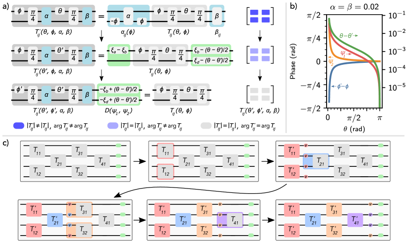
Figure 2: a) Fabrication-induced errors within each MZI can be corrected by applying local corrections $\theta\rightarrow\theta^{\prime}$, $\phi\rightarrow\phi^{\prime}$ to the device. We first correct $\theta$ to set the magnitudes of the elements of $T_{ij}$ equal to $T_{ij}^{\prime}$. Once the amplitude terms are set correctly, we apply phase corrections to the input and outputs of the device to correct phase errors between $T_{ij}$ and $T_{ij}^{\prime}.$ b) The corrections $\phi^{\prime}-\phi$, $\theta-\theta^{\prime}$, $\psi_{1}$, $\psi_{2}$ applied to an MZI with two 52-48 beamsplitters ($\alpha=\beta=0.02$). The arrows on the plot indicate which vertical axis each curve corresponds to. c) The procedure for programming a unitary with hardware errors on a $4\times 4$ rectangular unitary circuit. We first program each MZI to the $(\theta,\phi)$ setting obtained with the standard decomposition in [18]. Each MZI is then converted $T_{ij}\rightarrow T_{ij}^{\prime}$ to the settings for an imperfect device one column at a time. At each step we propagate the output phase shifts $\psi_{1},\psi_{2}$ forward in the circuit until the entire network is corrected.

Figure 2a illustrates our approach. We begin by finding $\theta^{\prime}$ such that the magnitudes of the entries of $T^{\prime}_{ij}(\theta^{\prime},\phi^{\prime},\alpha,\beta)$ equal those of $T_{ij}(\theta,\phi)$. This condition produces the following expression for $\theta^{\prime}$ (Supplementary Info., Sec. III.A.):

$$\theta^{\prime} =2\arcsin\sqrt{\frac{\sin^{2}(\theta/2)-\sin^{2}(\alpha+\beta)}{\cos^{2}(\alpha-\beta)-\sin^{2}(\alpha+\beta)}}$$ (8)

Component errors restrict the range over which $\theta$ is physically realizable. The above expression has a solution only if $\sin^{2}(\theta/2)>\sin^{2}(\alpha+\beta)$ and if $\sin^{2}(\theta/2)<\cos^{2}(\alpha-\beta)$. This restricts $\theta$ to the range:

$$2|\alpha+\beta|<\theta<\pi-2|\alpha-\beta|$$ (9)

If the matrix decomposition requires $\theta$ outside this range, the error is minimized by setting $\theta^{\prime}=0$ (if $\theta<2\lvert\alpha+\beta\rvert$) or $\theta^{\prime}=\pi$ (if $\theta>\pi-2\lvert\alpha-\beta\rvert$).

Assuming we can physically implement the required value of $\theta^{\prime}$, the magnitudes of the elements of $T^{\prime}_{ij}(\theta^{\prime},\phi^{\prime},\alpha,\beta)$ and $T_{ij}(\theta,\phi)$ are now the same, but each element of $T^{\prime}_{ij}$ will have an undesired extraneous phase $\xi_{a},\xi_{b},\xi_{c},\xi_{d}$ relative to the corresponding term in $T_{ij}$ that must be corrected. We can therefore rewrite $T^{\prime}_{ij}(\theta^{\prime},\phi^{\prime},\alpha,\beta)$ as

$$T^{\prime}_{ij} =ie^{i\theta^{\prime}/2}\begin{bmatrix}e^{i\phi^{\prime}}e^{i\xi_{a}}\sin(\theta/2)&e^{i\xi_{b}}\cos(\theta/2)\\ e^{i\phi^{\prime}}e^{i\xi_{c}}\cos(\theta/2)&-e^{i\xi_{d}}\sin(\theta/2)\end{bmatrix}$$ (10)

$$=ie^{i\theta^{\prime}/2}\begin{bmatrix}e^{i\xi_{b}}&0\\ 0&e^{i\xi_{d}}\end{bmatrix}\begin{bmatrix}e^{i(\phi^{\prime}+\xi_{a}-\xi_{b})}\sin(\theta/2)&\cos(\theta/2)\\ e^{i(\phi^{\prime}+\xi_{a}-\xi_{b})}\cos(\theta/2)&-\sin(\theta/2)\end{bmatrix}$$ (11)

where the simplification in the second line originates from unitarity requiring that $\xi_{a}+\xi_{d}=\xi_{b}+\xi_{c}$. We correct the phase errors in $T^{\prime}_{ij}$ by setting $\phi^{\prime}=\phi+\xi_{b}-\xi_{a}$ and by applying additional phases $\psi_{1}=-\xi_{b}+(\theta-\theta^{\prime})/2$, $\psi_{2}=-\xi_{d}+(\theta-\theta^{\prime})/2$ to the top and bottom output modes, respectively. Applying these corrections will set $T^{\prime}_{ij}(\theta^{\prime},\phi^{\prime},\alpha,\beta)$ exactly equal to $T_{ij}(\theta,\phi)$.

Expressions for the phase errors $\xi_{a},\xi_{b},\xi_{d}$ can be constructed by setting the complex arguments of the elements of $T_{ij}$ equal to those of $T^{\prime}_{ij}(\theta^{\prime},\phi^{\prime},\alpha,\beta)$. From this, we find that:

$$\phi^{\prime}=\phi +\arctan\left[\frac{\sin(\alpha-\beta)}{\cos(\alpha+\beta)}\tan(\theta^{\prime}/2)\right]$$

$$-\arctan\left[\frac{\sin(\alpha+\beta)}{\cos(\alpha-\beta)}\cot(\theta^{\prime}/2)\right]$$ (12)

$$\psi_{1}=-\arctan\left[\frac{\sin(\alpha-\beta)}{\cos(\alpha+\beta)}\tan(\theta^{\prime}/2)\right]+(\theta-\theta^{\prime})/2$$ (13)

$$\psi_{2}=\arctan\left[\frac{\sin(\alpha+\beta)}{\cos(\alpha-\beta)}\cot(\theta^{\prime}/2)\right]+(\theta-\theta^{\prime})/2$$ (14)

The errors $\theta-\theta^{\prime},\phi^{\prime}-\phi,\psi_{1},\psi_{2}$ as a function of $\theta$ for an example MZI with two 52-48 ($\alpha=\beta=0.02$) splitters are shown in Figure 2b. While the corrections to $\theta$ and $\psi_{1}$ are small ($\sim 0.1$ rad), the errors for $\phi$ and $\psi_{2}$ are quite substantial. In particular, for low device reflectivities ($\theta\approx 0$), the phase corrections required can exceed 1 rad.

Generally, we cannot apply the auxiliary phases $\psi_{1},\psi_{2}$ locally to the device being corrected, since the output modes do not have phase shifters. In most cases, one of the two can be incorporated into the external phase shifter setting of an MZI in the subsequent column. The other phase can be applied by observing that:

$$T_{ij}(\theta,\phi)\begin{bmatrix}e^{i\psi_{1}}&0\\ 0&e^{i\psi_{2}}\end{bmatrix}=\begin{bmatrix}e^{i\psi_{2}}&0\\ 0&e^{i\psi_{2}}\end{bmatrix}T_{ij}(\theta,\phi+\psi_{1}-\psi_{2})$$ (15)

Using this fact, we can propagate the auxiliary phases forward, through all of the columns of the network, out to the phase shifters $D$ located on the output modes of the circuit. This procedure, illustrated in Figure 2c, produces a modified output phase screen $D^{\prime}$ such that:

$$U=D\prod T_{ij}(\theta,\phi)=D^{\prime}\prod T^{\prime}_{ij}(\theta^{\prime},\phi^{\prime},\alpha,\beta)$$ (16)

Depending on the component imperfections and the required value of $\theta$, we may also be able to program $\theta^{\prime}$ such that $|T^{\prime}_{ij}(\theta^{\prime},\phi^{\prime},\alpha,\beta)|=|T_{ij}(\theta,\phi)|$ if the condition in equation (9) is satisfied. If every MZI in the circuit satisfies the condition in equation (9), we can recover the exact unitary desired. However, if some MZIs in the circuit cannot realize the required splitting, that exact unitary is not physically realizable by the device. In this case, correcting the phases $\phi^{\prime},\psi_{1},\psi_{2}$ and setting $\theta^{\prime}$ as close to the required value as possible minimizes the gate error $\lVert T_{ij}-T^{\prime}_{ij}\rVert$.

We can summarize the algorithm for programming of a matrix $U$ as follows:

1. Calculate the required values for $\theta,\phi$ assuming ideal components, using the procedure described by Reck [17] or Clements [18].

2. For each device, set $\theta\rightarrow\theta^{\prime}$ using the expression in equation (8). If $\theta<2|\alpha+\beta|$, set $\theta^{\prime}=0$; if $\theta>\pi-2\lvert\alpha-\beta\rvert$, set $\theta^{\prime}=\pi$.

3. Apply phase corrections $\phi^{\prime},\psi_{1},\psi_{2}$ as given in equations 12-14. Propagate $\psi_{1},\psi_{2}$ forward to the output phase screen $D$ with the expression in equation (15).

We have illustrated this procedure for the example of feedforward unitary circuits, but the same principles apply for other architectures. Each optical gate within any programmable circuit can be corrected to the required $2\times 2$ unitary operation $T_{ij}$ with the aforementioned procedure. The expressions provided assume a specific form for the MZI (Fig. 1), but they can be easily modified to apply to other designs, such as the dual-drive tunable basic unit (TBU) used in recirculating architectures [33].

3 Discussion

3.1 Hardware Performance

We analyzed the performance of error correction through numerical simulations of programmable photonic circuits with fabrication imperfections. Results were obtained with a custom simulation package written using NumPy [34]. Further details are included in the Supplementary Information.

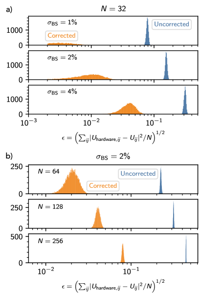
Figure 3: a) Matrix error $\epsilon$ before and after correction for 100 random unitaries implemented on 100 random circuits with varying beamsplitter statistics. b) Matrix error $\epsilon$ before and after correction for $N=\{64,128,256\}$ with a beamsplitter variation $\sigma_{BS}=2\%$.

Figure 3a shows the matrix error (relative error per entry) $\epsilon=(\sum_{ij}\lvert U_{\text{hardware},ij}-U_{ij}\rvert^{2}/N)^{1/2}$ for 100 Haar random unitaries implemented on 100 randomly generated $N=32$-mode unitary circuits with mean beamsplitter transmission $\eta=(50\pm\sigma_{\text{BS}})\%$. The beamsplitter errors are independently sampled from a Gaussian distribution; for large $N$, the distribution shape will not greatly affect the results. We find that error correction reduces $\epsilon$ significantly, sometimes by more than an order of magnitude. This improvement is larger for circuits with small splitting errors, as they are more likely to satisfy equation (9) and program the required $\theta^{\prime}$ for all devices within the circuit. However, even for circuits with large $\sigma_{\text{BS}}$, where many MZIs may not be programmable to the required $\theta$, the improvement in $\epsilon$ is substantial as all errors in $\phi,\psi_{1},\psi_{2}$ can always be corrected.

In Figure 3b, we show $\epsilon$ with and without error correction for circuit sizes $N=\{64,128,256\}$. For these simulations, we chose a beamsplitter variation of $\sigma_{BS}=2\%$, which is a typical wafer-level variance [19]. While the improvement in $\epsilon$ diminishes for larger $N$, we still find substantial improvement gained in our approach for up to 256 modes. For large unitary circuits most MZIs need to be programmed to reflectivities close to $\theta\approx 0$ [35]; the increasing fraction of devices that cannot be programmed to the required splitting accounts for the increase in $\epsilon$ with $N$. Nevertheless, there is always some improvement in $\epsilon$, as any phase errors introduced by the components can be corrected. Our results suggest that substantial performance improvements can still be achieved by error correction for circuits with hundreds of modes, which is well beyond the size of the current state-of-the-art ($N=64$) in programmable photonics [36].

3.2 Application: Optical Neural Networks on Feedforward Programmable Circuits

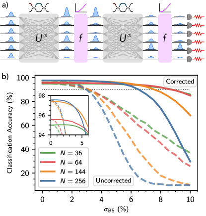
Figure 4: a) We simulated the effect of component error on two-layer optical neural networks for the MNIST task. Matrix-vector products are calculated optically in the photonic circuit, and modReLU-like activation functions are implemented electro-optically [37, 38]. b) Median accuracy for 300 unitary circuits as a function of $\sigma_{BS}$ with and without correction for a photonic image classifier for the MNIST task with $N=\{36,64,144,256\}$ neurons. Error correction significantly improves the fabrication tolerance of the neural network to beyond current-day process tolerances, even for systems with hundreds of modes. As the inset shows, even circuits with 4% splitter error preserve the baseline performance within 1%.

To further benchmark the performance of our error correction protocol, we applied this approach to simulations of a programmable photonic system, namely a two-layer neural network conducting inference with a feedforward programmable photonic circuit. The architecture of the neural network is similar to that studied in [16, 32, 20], where forward inference is optically computed through passive interference within a unitary photonic circuit coupled with an electrical or electro-optic nonlinearity [38]. Optical machine learning is a key application area for photonic error correction, as model training is both time-consuming and energy intensive, making it impractical to retrain on each individual piece of hardware with a unique set of fabrication errors. Preferably, a model would be highly optimized once in software, after which corrections are applied within the hardware to restore the original software-trained model from any fabrication-induced errors.

The neural networks we benchmark are based on the architecture described in [32]. Using the Neurophox package, we trained two-layer neural networks with $N=\{36,64,144,256\}$ neurons to recognize low-frequency Fourier features of handwritten digits from the MNIST task. The activation function between layers was assumed to be a modReLU function implemented using an electro-optic nonlinearity [37, 38]. Further details on the network architecture and training are included in the Supplementary Information.

Figure 4 shows the median classification accuracy for 300 randomly generated circuits as a function of the beamsplitter statistics $\eta=(50\pm\sigma_{\text{BS}})\%$. The smaller circuits ($N=36,64$) exhibit roughly $95-96\%$ accuracy after training, while the larger circuits ($N=144,256$) exhibit a slightly higher model accuracy of $\sim 97\%$. The larger circuits, however, are less resilient to errors; without error correction classification accuracy drops to below 90% for all circuit sizes at a splitter variation as low as $\sim 3\%$.

Hardware error correction extends this cutoff to more than $6\%$, which is well beyond modern-day process tolerances [19]. Moreover, without correction classification accuracy drops significantly at even typical wafer-level variances (2%). However, with error correction there is almost no drop in accuracy at these variances and less than 1% accuracy loss for beamsplitter variations as high as 4%. We expect this margin for fabrication error will prove important as optical neural networks scale up. These results suggest that error correction in programmable photonics can enable high-accuracy neural networks of up to hundreds of modes within current-day process tolerances.

3.3 Application: Tunable Dispersion Compensators on Recirculating Waveguide Meshes

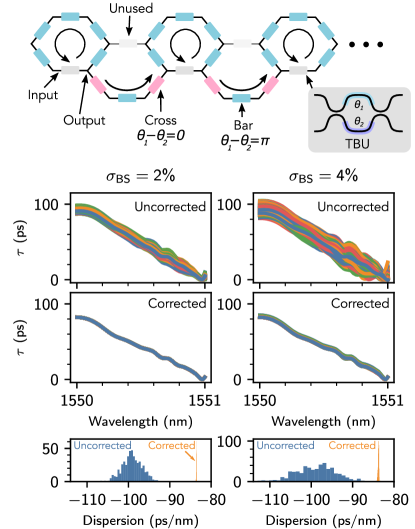
Figure 5: Top: Simulations of a tunable dispersion compensator (TDC) implemented on a recirculating waveguide mesh with 15 tunable-coupling ring resonators coupled serially to one another. Bottom: After training the mesh parameters to implement a fixed linear group delay dispersion on an ideal model, small beamsplitter errors will introduce variations in the implemented group delay $\tau$ profile. Plotted are the group delay profiles for 500 randomly generated circuits before and after correction. Correcting the settings of each TBU restores the desired performance, eliminating the need to retrain on the hardware. Also displayed is the distribution of the group delay dispersion before and after correction.

While our analysis has focused on feedforward programmable photonic meshes, our results can also be applied to recirculating architectures useful in RF and optical signal processing. These recirculating meshes, which are usually configured in hexagonal or triangular lattices, enable implementation of finite impulse response (FIR) and infinite impulse response (IIR) filters by configuring waveguides into asymmetric MZIs and ring resonators, respectively [13, 22, 21]. Unlike the feedforward architectures, the programming of these structures usually cannot be determined analytically and must be found through optimization [26, 27, 28]. Since optimization can be time-consuming for complex systems, error correction can enable optimizing these circuit parameters on idealized models and then porting them over to hardware without retraining. As an example, we simulated the performance of an IIR filter functioning as a tunable dispersion compensator (TDC) on a hexagonal waveguide lattice [22]. TDC modules are of interest for numerous applications, including compensating chromatic dispersion in optical communication links [39] and enabling high-dimensional quantum key distribution (QKD) with temporal modes [40].

We implemented the TDC using an architecture similar to the tunable-coupling ring array described in [14]. Programmable dispersion is achieved by individually tuning the coupling and resonance of each ring in a chain of 15 resonators coupled serially to one another. Each ring is implemented with a single MZI (often referred to as the tunable basic unit, or TBU) in a hexagonal mesh acting as the coupler, while five other TBUs are programmed to the bar state to implement feedback. For simplicity we do not simulate routing within the hexagonal mesh, but instead simulate the transfer function of each individual filter implemented using TBUs with fabrication imperfections. Using the constrained optimization by linear approximations (COBYLA) routine in SciPy [41, 42], we trained the TBU parameters on an idealized model to implement a group delay dispersion of $-85$ ps/nm over the bandwidth of a 50 GHz ITU channel.

Figure 5 shows the group delay $\tau$ profiles for 500 randomly generated TDC modules implemented using TBUs with $\sigma_{\text{BS}}=\{2,4\}\%$ before (top) and after (bottom) error correction. Similar to optical neural networks, precise implementation of a TDC requires accurate phase control throughout the circuit. Fabrication errors introduce spurious phases at each resonance, which results in significant variation of the dispersion profile for even slight component errors. As our results show, correcting the parameters of each TBU locally is sufficient to restore the desired dispersion profile.

While we can correct the coupling and phase parameters for each ring, errors $\alpha,\beta$ also introduce some loss at each TBU programmed to the bar state, as the bar transmission is reduced to $\cos^{2}(\alpha-\beta)$. The remainder of the light is directed into unused couplers in the circuit, effectively incurring loss. This alters the critical coupling condition, which results in the slight variation in the dispersion profile observed for $\sigma_{BS}=4\%$. Our simulations assume $\alpha,\beta$ are independent, Gaussian random variables; in practice, however, $\alpha,\beta$ for a single device are strongly correlated [43, 44]. Therefore, our simulations likely overestimate the loss incurred at each TBU programmed to the bar state.

3.4 Scalability and Outlook

We have presented an approach for characterizing and correcting for hardware errors in programmable photonic circuits. To conclude, we analyze the expected improvement our technique enables and how it will perform as these circuits scale up.

For a unitary photonic circuit, applying the Reck or Clements decompositions produces an average matrix error $\epsilon$ of (Supplementary Info., Sec. II.A.):

$$\langle\epsilon\rangle\approx\sigma_{BS}\sqrt{2(N-1)}$$ (17)

If we can correct all errors in $\theta$, then $\epsilon_{\text{corrected}}\rightarrow 0$. We can therefore estimate the expected $\epsilon_{\text{corrected}}$ by computing the fraction of MZIs that cannot be programmed to the required splitting value, i.e. the condition in equation (9).

The distribution of phase shifter settings for a unitary circuit can be related to the Haar measure on the unitary group [35]. The probability an MZI is programmed to a value $\theta<\xi$ is (Supplementary Info., Sec. II.C.):

$$P(\theta<\xi) =\sum_{k=1}^{N-1}\frac{2(N-k)}{N(N-1)}(1-\cos^{2k}(\xi/2))$$ (18)

$$\approx\frac{N+1}{12}\xi^{2}$$ (19)

We disregard the probability an MZI is programmed to a splitting $\theta>\pi-2|\alpha-\beta|$, which is negligibly small for large $N$ [35]. Error correction cannot fix the splitting error if $\theta<2\lvert\alpha+\beta\rvert$; therefore:

$$\langle\epsilon_{\text{corrected}}\rangle \approx\left(\frac{1}{2}P(\theta<2\lvert\alpha+\beta\rvert)\langle\epsilon^{2}\rangle\right)^{1/2}$$ (20)

$$=\sigma_{\text{BS}}^{2}\sqrt{\frac{2(N^{2}-1)}{3}}$$ (21)

We find that error correction effectively reduces the hardware error from $\epsilon$ to $\approx(1/\sqrt{6})\epsilon^{2}$. The expected error improvement is:

$$\frac{\langle\epsilon\rangle}{\langle\epsilon_{\text{corrected}}\rangle}\approx\frac{\sqrt{3}}{\sigma_{\text{BS}}\sqrt{N+1}}$$ (22)

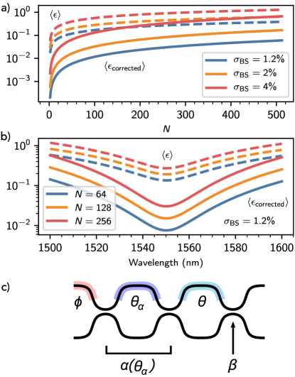
Figure 6: a) $\langle\epsilon\rangle,\langle\epsilon_{\text{corrected}}\rangle$ as a function of circuit size $N$ for $\sigma_{\text{BS}}=\{1.2,2,4\}\%$. b) Average circuit error as a function of wavelength for $N=\{64,128,256\}$ using the optimal directional coupler design in [19]. c) Redundant MZI for implementing perfect optical gates. One of the two beamsplitters is an MZI that can be tuned to implement an error $\alpha(\theta_{\alpha})$ which compensates for the error $\beta$.

$\langle\epsilon\rangle$ and $\langle\epsilon_{\text{corrected}}\rangle$ as a function of $N$ are plotted in Figure 6a. We consider $\sigma_{\text{BS}}=1.2\%$, which is the state-of-the-art reported in [19], as well as more relaxed tolerances $\sigma_{\text{BS}}=\{2,4\}\%$. For $\sigma_{\text{BS}}$ as high as 4%, error correction produces at least a factor of two (and often more) improvement in the error for circuits as large as $N=500$. We therefore expect our approach to have wide applicability in the near term as the size of programmable photonic circuits scale up.

Error correction also greatly improves the optical bandwidth of unitary circuits. Since directional couplers are highly wavelength sensitive, dense wavelength-division multiplexing (DWDM) requires re-fabricating the same circuit with components optimized at each wavelength channel. Our approach, however, enables the use of the same hardware across a wide wavelength range. In Figure 6b we show the expected hardware errors for large circuits across a 100 nm bandwidth using the optimal splitter ($\sigma_{\text{BS}}=1.2\%$) design in [19]. We find that the corrected error for an $N=256$ circuit across a 60 nm bandwidth (1520-1580 nm) will be lower than the uncorrected error at the design wavelength $\lambda=1550$ nm. Even lower errors could be achieved using multimode interference (MMI) couplers; these devices have large bandwidths but often suffer from static splitting imbalances [45], i.e., $\alpha,\beta$ are invariant to wavelength, but $\langle\alpha\rangle,\langle\beta\rangle\neq 0$. A circuit with large-bandwidth MMI couplers can thus use error correction to achieve a large instantaneous bandwidth, for instance to compute over many parallel wavelength channels.

The results in Figure 6a suggest a fundamental error bound achievable with local correction for unitary circuits. Our approach yields comparable results to those achieved with self-configuration procedures [9, 32] but does not require a specific structure for the circuit or photodiodes within each device. If the condition in equation (9) is satisfied, local correction obtains $\epsilon_{\text{corrected}}=0$ in $O(1)$ time. If this condition is not satisfied, it is sometimes possible to achieve a larger reduction in error with a global optimization approach [24, 29]. However, these approaches, which require photodiodes within each device or output measurements whose number scale nonlinearly with the number of modes, become increasingly inaccessible experimentally as N scales up. Local correction requires minimal overhead and can guarantee a minimum error given certain guarantees on the component performance, making it ideal for standardizing performance across large numbers of chips.

Moreover, this error bound applies only to feedforward, unitary circuits with no redundant devices. $\epsilon$ lower than this bound can be achieved by incorporating additional, redundant MZIs; for instance, one can implement “perfect” optical gates by incorporating an additional phase shifter into the MZI, as shown in Figure 6c. This device can be trained with optimization to implement any desired unitary $T_{ij}(\theta,\phi)$ perfectly [46, 47]. The error correction formalism enables calculation of these settings analytically. One of the two constituent splitters is a passive component with error $\beta$, while the other splitter is an MZI that implements a tunable error $\alpha(\theta_{\alpha})$. Any desired $2\times 2$ unitary with a required splitting $\theta$ can then be implemented by setting $\theta_{\alpha}$ such that $2\lvert\alpha(\theta_{\alpha})+\beta\rvert<\theta<2\lvert\alpha(\theta_{\alpha})-\beta\rvert$ and correcting the resultant phase errors (Supplementary Info., Sec. III.B.).

Not all optical gates within the circuit necessarily need to incorporate redundancy. High accuracy unitary circuits have been demonstrated by incorporating only a few extra MZIs into the circuit, which can be trained using nonlinear optimization [24] or gradient descent [29]. Error correction serves an important purpose for these circuits, as one can optimize the hardware settings once on an ideal model and port the settings over to many devices. For recirculating meshes the phase shifter settings are not constrained by the Haar measure, and so the benefit gained from error correction is not expected to diminish with increasing $N$. We therefore expect error correction to play an important role in scaling up the size of these circuits as well.

The motivation for photonic error correction assumes the hardware is re-programmed infrequently, for instance to implement a weight matrix in a neural network. Other applications, such as mode unscrambling, require real-time configuration robust to device error. We have recently discussed error-resilient self-configuration approaches in [48, 49].

4 Conclusion

In conclusion, we have presented a protocol to correct for hardware errors in programmable photonic circuits. Unlike optimization-based approaches, our protocol utilizes a one-time calibration procedure to flexibly implement any desired functionality up to the limits of the hardware. We find that applying our approach to key application areas of programmable photonics, such as optical neural networks and programmable coupled-ring systems, enables resilience to fabrication errors well beyond modern-day process tolerances. Error correction also greatly reduces the overhead for programmable photonics that require optimization to deduce the hardware settings, as it eliminates the need to retrain for each individual set of hardware with unknown fabrication errors. Current process tolerances suggest that our approach enables improved functionality for systems of up to hundreds of modes, providing a new avenue for scaling up programmable photonics.

Funding National Science Foundation (NSF) Graduate Research Fellowship Program (1745302); Air Force Office of Scientific Research (AFOSR) (FA9550-20-1-0113; FA9550-16-1-0391); IC Postdoctoral Research Fellowship Program.

Acknowledgments The authors are grateful to Hugo Larocque and Alexander Sludds for helpful comments on the manuscript.

Disclosures The authors are inventors on a provisional patent application on error correction methods for programmable photonics.

Data availability The data that support the plots in this paper are available from the corresponding author upon reasonable request.

Supplemental document See Supplement 1 for supporting content.

References

- [1] W. Bogaerts, D. Pérez, J. Capmany, D. A. B. Miller, J. Poon, D. Englund, F. Morichetti, and A. Melloni, “Programmable photonic circuits,” \JournalTitleNature 586, 207–216 (2020).
- [2] N. C. Harris, J. Carolan, D. Bunandar, M. Prabhu, M. Hochberg, T. Baehr-Jones, M. L. Fanto, A. M. Smith, C. C. Tison, P. M. Alsing, and D. Englund, “Linear programmable nanophotonic processors,” \JournalTitleOptica 5, 1623 (2018).
- [3] N. C. Harris, G. R. Steinbrecher, M. Prabhu, Y. Lahini, J. Mower, D. Bunandar, C. Chen, F. N. C. Wong, T. Baehr-Jones, M. Hochberg, S. Lloyd, and D. Englund, “Quantum transport simulations in a programmable nanophotonic processor,” \JournalTitleNature Photonics 11, 447–452 (2017).
- [4] J. Wang, S. Paesani, Y. Ding, R. Santagati, P. Skrzypczyk, A. Salavrakos, J. Tura, R. Augusiak, L. Mančinska, D. Bacco, D. Bonneau, J. W. Silverstone, Q. Gong, A. Acín, K. Rottwitt, L. K. Oxenløwe, J. L. O’Brien, A. Laing, and M. G. Thompson, “Multidimensional quantum entanglement with large-scale integrated optics,” \JournalTitleScience 360, 285–291 (2018).
- [5] X. Qiang, X. Zhou, J. Wang, C. M. Wilkes, T. Loke, S. O’Gara, L. Kling, G. D. Marshall, R. Santagati, T. C. Ralph, J. B. Wang, J. L. O’Brien, M. G. Thompson, and J. C. F. Matthews, “Large-scale silicon quantum photonics implementing arbitrary two-qubit processing,” \JournalTitleNature Photonics 12, 534–539 (2018).
- [6] C. Sparrow, E. Martín-López, N. Maraviglia, A. Neville, C. Harrold, J. Carolan, Y. N. Joglekar, T. Hashimoto, N. Matsuda, J. L. O’Brien, D. P. Tew, and A. Laing, “Simulating the vibrational quantum dynamics of molecules using photonics,” \JournalTitleNature 557, 660–667 (2018).
- [7] J. Carolan, C. Harrold, C. Sparrow, E. Martin-Lopez, N. J. Russell, J. W. Silverstone, P. J. Shadbolt, N. Matsuda, M. Oguma, M. Itoh, G. D. Marshall, M. G. Thompson, J. C. F. Matthews, T. Hashimoto, J. L. O’Brien, and A. Laing, “Universal linear optics,” \JournalTitleScience 349, 711–716 (2015).
- [8] D. A. B. Miller, “Self-configuring universal linear optical component,” \JournalTitlePhotonics Research 1, 1 (2013).
- [9] D. A. B. Miller, “Self-aligning universal beam coupler,” \JournalTitleOptics Express 21, 6360 (2013).
- [10] A. Annoni, E. Guglielmi, M. Carminati, G. Ferrari, M. Sampietro, D. A. Miller, A. Melloni, and F. Morichetti, “Unscrambling light—automatically undoing strong mixing between modes,” \JournalTitleLight: Science & Applications 6, e17110 (2017).
- [11] A. Ribeiro, A. Ruocco, L. Vanacker, and W. Bogaerts, “Demonstration of a 4 4-port universal linear circuit,” \JournalTitleOptica 3, 1348 (2016).
- [12] M. Milanizadeh, P. Borga, F. Morichetti, D. Miller, and A. Melloni, “Manipulating Free-space Optical Beams with a Silicon Photonic Mesh,” in 2019 IEEE Photonics Society Summer Topical Meeting Series (SUM), (2019), pp. 1–2.
- [13] L. Zhuang, C. G. H. Roeloffzen, M. Hoekman, K.-J. Boller, and A. J. Lowery, “Programmable photonic signal processor chip for radiofrequency applications,” \JournalTitleOptica 2, 854 (2015).
- [14] J. Notaros, J. Mower, M. Heuck, C. Lupo, N. C. Harris, G. R. Steinbrecher, D. Bunandar, T. Baehr-Jones, M. Hochberg, S. Lloyd, and D. Englund, “Programmable dispersion on a photonic integrated circuit for classical and quantum applications,” \JournalTitleOptics Express 25, 21275 (2017).
- [15] M. Prabhu, C. Roques-Carmes, Y. Shen, N. Harris, L. Jing, J. Carolan, R. Hamerly, T. Baehr-Jones, M. Hochberg, V. Čeperić, J. D. Joannopoulos, D. R. Englund, and M. Soljačić, “Accelerating recurrent Ising machines in photonic integrated circuits,” \JournalTitleOptica 7, 551 (2020).
- [16] Y. Shen, N. C. Harris, S. Skirlo, M. Prabhu, T. Baehr-Jones, M. Hochberg, X. Sun, S. Zhao, H. Larochelle, D. Englund, and M. Soljačić, “Deep learning with coherent nanophotonic circuits,” \JournalTitleNature Photonics 11, 441–446 (2017).
- [17] M. Reck, A. Zeilinger, H. J. Bernstein, and P. Bertani, “Experimental realization of any discrete unitary operator,” \JournalTitlePhysical Review Letters 73, 58–61 (1994).
- [18] W. R. Clements, P. C. Humphreys, B. J. Metcalf, W. S. Kolthammer, and I. A. Walsmley, “Optimal design for universal multiport interferometers,” \JournalTitleOptica 3, 1460 (2016).
- [19] J. C. Mikkelsen, W. D. Sacher, and J. K. S. Poon, “Dimensional variation tolerant silicon-on-insulator directional couplers,” \JournalTitleOptics Express 22, 3145 (2014).
- [20] M. Y.-S. Fang, S. Manipatruni, C. Wierzynski, A. Khosrowshahi, and M. R. DeWeese, “Design of optical neural networks with component imprecisions,” \JournalTitleOptics Express 27, 14009 (2019).
- [21] D. Pérez, I. Gasulla, and J. Capmany, “Field-programmable photonic arrays,” \JournalTitleOptics Express 26, 27265 (2018).
- [22] D. Pérez, I. Gasulla, J. Capmany, and R. A. Soref, “Reconfigurable lattice mesh designs for programmable photonic processors,” \JournalTitleOptics Express 24, 12093 (2016).
- [23] I. Zand and W. Bogaerts, “Effects of coupling and phase imperfections in programmable photonic hexagonal waveguide meshes,” \JournalTitlePhotonics Research 8, 211 (2020).
- [24] R. Burgwal, W. R. Clements, D. H. Smith, J. C. Gates, W. S. Kolthammer, J. J. Renema, and I. A. Walmsley, “Using an imperfect photonic network to implement random unitaries,” \JournalTitleOptics Express 25, 28236 (2017).
- [25] J. Mower, N. C. Harris, G. R. Steinbrecher, Y. Lahini, and D. Englund, “High-fidelity quantum state evolution in imperfect photonic integrated circuits,” \JournalTitlePhysical Review A 92, 032322 (2015).
- [26] A. López, D. Pérez, P. DasMahapatra, and J. Capmany, “Auto-routing algorithm for field-programmable photonic gate arrays,” \JournalTitleOptics Express 28, 737 (2020).
- [27] D. P. López, “Programmable Integrated Silicon Photonics Waveguide Meshes: Optimized Designs and Control Algorithms,” \JournalTitleIEEE Journal of Selected Topics in Quantum Electronics 26, 1–12 (2020).
- [28] D. Pérez-López, A. López, P. DasMahapatra, and J. Capmany, “Multipurpose self-configuration of programmable photonic circuits,” \JournalTitleNature Communications 11, 6359 (2020).
- [29] S. Pai, B. Bartlett, O. Solgaard, and D. A. B. Miller, “Matrix Optimization on Universal Unitary Photonic Devices,” \JournalTitlePhysical Review Applied 11, 064044 (2019).
- [30] T. W. Hughes, M. Minkov, Y. Shi, and S. Fan, “Training of photonic neural networks through in situ backpropagation and gradient measurement,” \JournalTitleOptica 5, 864 (2018).
- [31] D. A. B. Miller, “Setting up meshes of interferometers – reversed local light interference method,” \JournalTitleOptics Express 25, 29233 (2017).
- [32] S. Pai, I. A. D. Williamson, T. W. Hughes, M. Minkov, O. Solgaard, S. Fan, and D. A. B. Miller, “Parallel Programming of an Arbitrary Feedforward Photonic Network,” \JournalTitleIEEE Journal of Selected Topics in Quantum Electronics 26, 1–13 (2020).
- [33] D. Pérez-López, A. M. Gutierrez, E. Sánchez, P. DasMahapatra, and J. Capmany, “Integrated photonic tunable basic units using dual-drive directional couplers,” \JournalTitleOptics Express 27, 38071 (2019).
- [34] C. R. Harris, K. J. Millman, S. J. van der Walt, R. Gommers, P. Virtanen, D. Cournapeau, E. Wieser, J. Taylor, S. Berg, N. J. Smith, R. Kern, M. Picus, S. Hoyer, M. H. van Kerkwijk, M. Brett, A. Haldane, J. F. del R’ıo, M. Wiebe, P. Peterson, P. G’erard-Marchant, K. Sheppard, T. Reddy, W. Weckesser, H. Abbasi, C. Gohlke, and T. E. Oliphant, “Array programming with NumPy,” \JournalTitleNature 585, 357–362 (2020).
- [35] N. J. Russell, L. Chakhmakhchyan, J. L. O’Brien, and A. Laing, “Direct dialling of Haar random unitary matrices,” \JournalTitleNew Journal of Physics 19, 033007 (2017).
- [36] N. C. Harris, R. Braid, D. Bunandar, J. Carr, B. Dobbie, C. Dorta-Quinones, J. Elmhurst, M. Forsythe, M. Gould, S. Gupta, S. Kannan, T. Kenney, G. Kong, T. Lazovich, S. Mckenzie, C. Ramey, C. Ravi, M. Scott, J. Sweeney, O. Yildirim, and K. Zhang, “Accelerating artificial intelligence with silicon photonics,” in Optical Fiber Communication Conference (OFC) 2020, (OSA, San Diego, California, 2020), p. W3A.3.
- [37] M. Arjovsky, A. Shah, and Y. Bengio, “Unitary Evolution Recurrent Neural Networks,” in Proceedings of The 33rd International Conference on Machine Learning, vol. 48 of Proceedings of Machine Learning Research (PMLR, New York, New York, USA, 2016), pp. 1120–1128.
- [38] I. A. D. Williamson, T. W. Hughes, M. Minkov, B. Bartlett, S. Pai, and S. Fan, “Reprogrammable Electro-Optic Nonlinear Activation Functions for Optical Neural Networks,” \JournalTitleIEEE Journal of Selected Topics in Quantum Electronics 26, 1–12 (2020).
- [39] C. K. Madsen and G. Lenz, “Optical all-pass filters for phase response design with applications for dispersion compensation,” \JournalTitleIEEE Photonics Technology Letters 10, 994–996 (1998).
- [40] J. Mower, Z. Zhang, P. Desjardins, C. Lee, J. H. Shapiro, and D. Englund, “High-dimensional quantum key distribution using dispersive optics,” \JournalTitlePhysical Review A 87, 062322 (2013).
- [41] M. J. D. Powell, “Direct search algorithms for optimization calculations,” \JournalTitleActa Numerica 7, 287–336 (1998).
- [42] P. Virtanen, R. Gommers, T. E. Oliphant, M. Haberland, T. Reddy, D. Cournapeau, E. Burovski, P. Peterson, W. Weckesser, J. Bright, S. J. van der Walt, M. Brett, J. Wilson, K. J. Millman, N. Mayorov, A. R. J. Nelson, E. Jones, R. Kern, E. Larson, C. J. Carey, İ. Polat, Y. Feng, E. W. Moore, J. VanderPlas, D. Laxalde, J. Perktold, R. Cimrman, I. Henriksen, E. A. Quintero, C. R. Harris, A. M. Archibald, A. H. Ribeiro, F. Pedregosa, P. van Mulbregt, and SciPy 1.0 Contributors, “SciPy 1.0: Fundamental Algorithms for Scientific Computing in Python,” \JournalTitleNature Methods 17, 261–272 (2020).
- [43] Y. Yang, Y. Ma, H. Guan, Y. Liu, S. Danziger, S. Ocheltree, K. Bergman, T. Baehr-Jones, and M. Hochberg, “Phase coherence length in silicon photonic platform,” \JournalTitleOptics Express 23, 16890 (2015).
- [44] Z. Lu, J. Jhoja, J. Klein, X. Wang, A. Liu, J. Flueckiger, J. Pond, and L. Chrostowski, “Performance prediction for silicon photonics integrated circuits with layout-dependent correlated manufacturing variability,” \JournalTitleOptics Express 25, 9712 (2017).
- [45] H. Guan, Y. Ma, R. Shi, X. Zhu, R. Younce, Y. Chen, J. Roman, N. Ophir, Y. Liu, R. Ding, T. Baehr-Jones, K. Bergman, and M. Hochberg, “Compact and low loss 90∘ optical hybrid on a silicon-on-insulator platform,” \JournalTitleOptics Express 25, 28957 (2017).
- [46] K. Suzuki, G. Cong, K. Tanizawa, S.-H. Kim, K. Ikeda, S. Namiki, and H. Kawashima, “Ultra-high-extinction-ratio 2 × 2 silicon optical switch with variable splitter,” \JournalTitleOptics Express 23, 9086 (2015).
- [47] M. Wang, A. Ribero, Y. Xing, and W. Bogaerts, “Tolerant, broadband tunable 2 × 2 coupler circuit,” \JournalTitleOptics Express 28, 5555 (2020).
- [48] R. Hamerly, S. Bandyopadhyay, and D. Englund, “Stability of Self-Configuring Large Multiport Interferometers,” \JournalTitlein preparation (2021).
- [49] R. Hamerly, S. Bandyopadhyay, and D. Englund, “Accurate Self-Configuration of Rectangular Multiport Interferometers,” \JournalTitlein preparation (2021).