The effects of Vadasz term, anisotropy and rotation on bi-disperse convection

Abstract

The onset of thermal convection in a uniformly rotating and horizontally isotropic bi-disperse porous medium, taking into account the Vadasz term, is investigated. Via linear instability analysis, it has been proven that the Vadasz term allows the onset of convection via an oscillatory state but does not affect convection via a stationary motion.

Keywords Anisotropy  $\cdot$ Bi-disperse Porous Media  $\cdot$ Rotating Layer  $\cdot$ Vadasz Term  $\cdot$ Instability analysis

1 Introduction

A bi-disperse porous medium (BDPM) is a dual porosity material characterized by a standard pore structure, but the solid skeleton has fractures or cracks in it. In particular, a BDPM is a compound of clusters of large particles that are themselves aggregations of smaller particles: the macropores between the clusters are referred to as f-phase (meaning fracture phase) and have porosity $\varphi$, while the remainder of the structure is referred to as p-phase (meaning porous phase) and the porosity of the micropores within the clusters is $\epsilon$ [15].

While thermal convection has been widely studied in both clear fluid and porous media by many authors (see for example [6, 7, 8, 11, 12, 21, 22] and references therein), in the past as nowadays, double porosity materials has recently attracted many researchers due to their applications in engineering, medical field, chemistry (see [9, 10, 16] and references therein) and a theoretical key development is attributable to Nield and Kuznetsov in [13, 14, 15]. Bi-disperse porous media may be pretty useful in a laboratory [15], but in particular anisotropic bi-disperse porous materials offer much more possibilities to design man-made materials for heat transfer or insulation problems [4, 17, 20].
The analysis of fluid motion in rotating porous media finds many applications in geophysics and in engineering, for example for rotating machinery, chemical process industry, centrifugal filtration processes (see [21] and references therein), hence the study of thermal convection in rotating BDPM may be necessary and useful as well (see [3, 4, 5]).
Regarding the Vadasz term effect, it has been largely analysed by many authors in single porosity media (see for instance [1, 2, 6, 11, 22]) since the Vadasz number has a remarkable effect on the onset of convection in a rotating porous layer, in particular in [22] it has been proved that the Vadasz term leads to the onset of convection via an oscillatory state. On the other hand, the effect of Vadasz number on the onset of bi-disperse convection has been investigated by Straughan in [19], where he considered a fluid mixture saturating a BDPM, and by Capone and De Luca in [5], which deals with an isotropic and rotating BDPM.

The goal of the present paper is to analyse the combined effects of anisotropic permeabilities, uniform rotation about a vertical axis and inertia on the onset of thermal convection in an incompressible fluid saturating a single temperature bi-disperse porous medium. The paper is organized as follows. In section 2 the mathematical model and the associated perturbation equations are introduced. In section 3 we perform linear instability analysis of the thermal conduction solution, in particular, we find out that the Vadasz term allows the onset of thermal convection via an oscillatory state (named as oscillatory convection), but it does not affect the onset of thermal convection via a steady state (named as stationary convection). In sections 3.1 and 3.2 we determine the critical Rayleigh numbers for the onset of steady and oscillatory convection, respectively. In section 4 we perform numerical simulations in order to analyse the behaviour of the instability thresholds with respect to fundamental parameters. The paper ends with a concluding section that recaps all the results.

2 Mathematical model

Let $Oxyz$ be a reference frame with fundamental unit vectors ${\bf i,j,k}$ and let us assume that the plane layer $L$, of thickness $d$, of saturated bi-disperse porous medium is uniformly heated from below and rotates about the vertical axis $z$, let ${\bf\Omega}=\Omega{\bf k}$ be the constant angular velocity of the layer. Furthermore, we consider a single temperature bi-disperse porous medium, i.e. $T^{f}=T^{p}=T$. We restrict our attention to the case in which the permeabilities of the saturated bi-disperse porous medium are horizontally isotropic.
Let the axes $(x,y,z)$ be the principal axes of the permeabilities, so the macropermeability tensor and the micropermeability tensor may be written as

$${\bf K}^{f}=\text{diag}(K^{f}_{x},K^{f}_{y},K^{f}_{z})=K^{f}_{z}\ {\bf K}^{f*},$$

$${\bf K}^{p}=\text{diag}(K^{p}_{x},K^{p}_{y},K^{p}_{z})=K^{p}_{z}\ {\bf K}^{p*},$$

$${\bf K}^{f*}=\text{diag}(k,k,1),$$

$${\bf K}^{p*}=\text{diag}(h,h,1),$$

where

$$k=\frac{K^{f}_{x}}{K^{f}_{z}}=\frac{K^{f}_{y}}{K^{f}_{z}},$$

$$h=\frac{K^{p}_{x}}{K^{p}_{z}}=\frac{K^{p}_{y}}{K^{p}_{z}}.$$

Darcy’s model, with the Oberbeque-Boussinesq approximation, is employed, in particular it is extended in both micropores and macropores in order to include the Coriolis terms and is extended only in the macropores to include the time derivative term of the seepage velocity (see [5, 19]). The equations describing the evolutionary behaviour of thermal convection in a rotating horizontally isotropic bi-disperse porous medium are, cf. [3, 5],

$$\begin{cases}\varrho_{F}c_{a}\dfrac{\partial{\bf v}^{f}}{\partial t}=-\mu({\bf K}^{f})^{-1}{\bf v}^{f}-\zeta({\bf v}^{f}-{\bf v}^{p})-\nabla p^{f}+\varrho_{F}\alpha gT{\bf k}-\dfrac{2\varrho_{F}\Omega}{\varphi}{\bf k}\times{\bf v}^{f},\\ -\mu({\bf K}^{p})^{-1}{\bf v}^{p}-\zeta({\bf v}^{p}-{\bf v}^{f})-\nabla p^{p}+\varrho_{F}\alpha gT{\bf k}-\dfrac{2\varrho_{F}\Omega}{\epsilon}{\bf k}\times{\bf v}^{p}={\bf 0},\\ \nabla\cdot{\bf v}^{f}=0,\\ \nabla\cdot{\bf v}^{p}=0,\\ (\varrho c)_{m}\dfrac{\partial T}{\partial t}+(\varrho c)_{f}({\bf v}^{f}+{\bf v}^{p})\cdot\nabla T=k_{m}\Delta T,\end{cases}$$ (1)

where

$$p^{s}=P^{s}-\frac{\varrho_{F}}{2}|{\bf\Omega}\times{\bf x}|^{2},\quad s=\{f,p\}$$

are the reduced pressures, ${\bf x}=(x,y,z)$, ${\bf v}^{s}$ = seepage velocity for $s=\{f,p\}$, $\zeta$ = interaction coefficient between the f-phase and the p-phase, ${\bf g}=-g{\bf k}$ = gravity, $\mu$ = fluid viscosity, $\varrho_{F}$ = reference constant density, $\alpha$ = thermal expansion coefficient, $c$ = specific heat, $c_{p}$ = specific heat at a constant pressure, $c_{a}$= acceleration coefficient, $(\varrho c)_{m}=(1-\varphi)(1-\epsilon)(\varrho c)_{sol}+\varphi(\varrho c)_{f}+\epsilon(1-\varphi)(\varrho c)_{p}$, $k_{m}=(1-\varphi)(1-\epsilon)k_{sol}+\varphi k_{f}+\epsilon(1-\varphi)k_{p}$ = thermal conductivity (the subscript $sol$ is referred to the solid skeleton).

To 1 the following boundary conditions are appended

$$\begin{array}[]{l}{\bf v}^{s}\cdot{\bf n}=0\ \text{on}\ z=0,d,\ \text{for}\ s=\{f,p\}\\ T=T_{L}\ \text{on}\ z=0,\quad T=T_{U}\ \text{on}\ z=d,\end{array}$$ (2)

where ${\bf n}$ is the unit outward normal to the impermeable horizontal planes delimiting the layer and $T_{L}>T_{U}$.

System $(\ref{sist1})$-$(\ref{BC1})$ admits the stationary conduction solution:

$${\bf\overline{v}}^{f}=0,\ {\bf\overline{v}}^{p}=0,\ \overline{T}=-\beta z+T_{L},$$

where $\beta=\dfrac{T_{L}-T_{U}}{d}$ is the temperature gradient. Denoting by $\{{\bf u}^{f},{\bf u}^{p},\theta,\pi^{f},\pi^{p}\}$ a generic perturbation to the steady solution, the resulting perturbation equations are

$$\begin{cases}\varrho_{F}c_{a}\dfrac{\partial{\bf u}^{f}}{\partial t}=-\mu({\bf K}^{f})^{-1}{\bf u}^{f}-\zeta({\bf u}^{f}-{\bf u}^{p})-\nabla\pi^{f}+\varrho_{F}\alpha g\theta{\bf k}-\dfrac{2\varrho_{F}\Omega}{\varphi}{\bf k}\times{\bf u}^{f},\\ -\mu({\bf K}^{p})^{-1}{\bf u}^{p}-\zeta({\bf u}^{p}-{\bf u}^{f})-\nabla\pi^{p}+\varrho_{F}\alpha g\theta{\bf k}-\dfrac{2\varrho_{F}\Omega}{\epsilon}{\bf k}\times{\bf u}^{p}={\bf 0},\\ \nabla\cdot{\bf u}^{f}=0,\\ \nabla\cdot{\bf u}^{p}=0,\\ (\varrho c)_{m}\dfrac{\partial\theta}{\partial t}+(\varrho c)_{f}({\bf u}^{f}+{\bf u}^{p})\cdot\nabla\theta=(\varrho c)_{f}\beta(w^{f}+w^{p})+k_{m}\Delta\theta.\end{cases}$$ (3)

where ${\bf u}^{f}=(u^{f},v^{f},w^{f})$ and ${\bf u}^{p}=(u^{p},v^{p},w^{p})$. The above system $(\ref{pertsist})$ may be non-dimensionalized with the following non-dimensional parameters

$$\begin{array}[]{l}{\bf x}^{*}=\dfrac{{\bf x}}{d},\ t^{*}=\dfrac{t}{\tilde{t}},\ \theta^{*}=\dfrac{\theta}{\tilde{T}},\\ {\bf u}^{s*}=\dfrac{{\bf u}^{s}}{\tilde{u}},\ \pi^{s*}=\dfrac{\pi^{s}}{\tilde{P}},\ \text{for}\ s=\{f,p\}\\ \eta=\dfrac{\varphi}{\epsilon},\ \gamma=\dfrac{K^{f}_{z}\zeta}{\mu},\ K_{r}=\dfrac{K^{f}_{z}}{K^{p}_{z}},\end{array}$$

where the scales are given by

$$\tilde{u}=\frac{k_{m}}{(\varrho c)_{f}d},\ \tilde{t}=\frac{d^{2}(\varrho c)_{m}}{k_{m}},\ \tilde{P}=\frac{\mu k_{m}}{(\varrho c)_{f}K_{z}^{f}},\ \tilde{T}=\sqrt{\frac{\beta k_{m}\mu}{(\varrho c)_{f}\varrho_{F}\alpha gK_{z}^{f}}}.$$

The resulting non-dimensional perturbation equations, dropping all the asterisks, are

$$\begin{cases}-J\dfrac{\partial{\bf u}^{f}}{\partial t}-({\bf K}^{f})^{-1}{\bf u}^{f}-\gamma({\bf u}^{f}-{\bf u}^{p})-\nabla\pi^{f}+R\theta{\bf k}-\mathcal{T}{\bf k}\times{\bf u}^{f}={\bf 0},\\ -K_{r}({\bf K}^{p})^{-1}{\bf u}^{p}-\gamma({\bf u}^{p}-{\bf u}^{f})-\nabla\pi^{p}+R\theta{\bf k}-\eta\mathcal{T}{\bf k}\times{\bf u}^{p}={\bf 0},\\ \nabla\cdot{\bf u}^{f}=0,\\ \nabla\cdot{\bf u}^{p}=0,\\ \dfrac{\partial\theta}{\partial t}+({\bf u}^{f}+{\bf u}^{p})\cdot\nabla\theta=w^{f}+w^{p}+\Delta\theta,\end{cases}$$ (4)

where the Taylor number $\mathcal{T}$, the Vadasz number $J$ and the Rayleigh number $R$ are

$$\mathcal{T}=\dfrac{2\varrho_{F}\Omega K^{f}_{z}}{\varphi\mu},\qquad J=\dfrac{K^{f}_{z}\varrho_{F}c_{a}k_{m}}{\mu d^{2}(\varrho c)_{m}},\qquad R=\sqrt{\dfrac{\beta d^{2}(\varrho c)_{f}\varrho_{F}\alpha gK_{z}^{f}}{k_{m}\mu}}.$$

To system $(\ref{pertubations})$ the following initial and boundary conditions are appended:

$${\bf u}^{s}({\bf x},0)={\bf u}^{s}_{0}({\bf x}),\quad\pi^{s}({\bf x},0)=\pi^{s}_{0}({\bf x}),\quad\theta({\bf x},0)=\theta_{0}({\bf x}),$$

with $\nabla\cdot{\bf u}^{s}_{0}=0$, for $s=\{f,p\}$, and

$$w^{f}=w^{p}=\theta=0\quad\text{on}\ z=0,1.$$ (5)

According to experimental results, the solutions are required to be periodic in the horizontal directions $x$ and $y$ and in the sequel we will denote by

$$V=\Big{[}0,\frac{2\pi}{l}\Big{]}\times\Big{[}0,\frac{2\pi}{m}\Big{]}\times[0,1]$$

the periodicity cell.

3 Onset of convection

In order to determine the linear instability threshold of the thermal conduction solution, let us linearise system $(\ref{pertubations})$, i.e.

$$\begin{cases}-J\dfrac{\partial{\bf u}^{f}}{\partial t}-({\bf K}^{f})^{-1}{\bf u}^{f}-\gamma({\bf u}^{f}-{\bf u}^{p})-\nabla\pi^{f}+R\theta{\bf k}-\mathcal{T}{\bf k}\times{\bf u}^{f}={\bf 0},\\ -K_{r}({\bf K}^{p})^{-1}{\bf u}^{p}-\gamma({\bf u}^{p}-{\bf u}^{f})-\nabla\pi^{p}+R\theta{\bf k}-\eta\mathcal{T}{\bf k}\times{\bf u}^{p}={\bf 0},\\ \nabla\cdot{\bf u}^{f}=0,\\ \nabla\cdot{\bf u}^{p}=0,\\ \dfrac{\partial\theta}{\partial t}=w^{f}+w^{p}+\Delta\theta.\end{cases}$$ (6)

Being the system $(\ref{pertLIN})$ autonomous, we seek solutions with time-dependence like $e^{\sigma t}$, i.e.

$${\bf u}^{s}(t,{\bf x}) =e^{\sigma t}{\bf u}^{s}({\bf x}),$$ (7)

$$\theta(t,{\bf x}) =e^{\sigma t}\theta({\bf x}),$$

$$\pi^{s}(t,{\bf x}) =e^{\sigma t}\pi^{s}({\bf x}),$$

with $\sigma\in\mathbb{C}$ and $s=\{f,p\}$. By virtue of $(\ref{sol})$, $(\ref{pertLIN})$ becomes

$$\begin{cases}-J\sigma{\bf u}^{f}-({\bf K}^{f})^{-1}{\bf u}^{f}-\gamma({\bf u}^{f}-{\bf u}^{p})-\nabla\pi^{f}+R\theta{\bf k}-\mathcal{T}{\bf k}\times{\bf u}^{f}={\bf 0},\\ -K_{r}({\bf K}^{p})^{-1}{\bf u}^{p}-\gamma({\bf u}^{p}-{\bf u}^{f})-\nabla\pi^{p}+R\theta{\bf k}-\eta\mathcal{T}{\bf k}\times{\bf u}^{p}={\bf 0},\\ \nabla\cdot{\bf u}^{f}=0,\\ \nabla\cdot{\bf u}^{p}=0,\\ \sigma\theta=w^{f}+w^{p}+\Delta\theta.\end{cases}$$ (8)

Setting

$$\omega^{s}_{3}=(\nabla\times{\bf u}^{s})\cdot{\bf k},\,\,s=\{f,p\},$$

let us consider the third components of the curl and of the double curl of $(\ref{pert})_{1,2}$, i.e.

$$\begin{cases}(J\sigma+\dfrac{1}{k}+\gamma)\omega_{3}^{f}-\gamma\omega^{p}_{3}-\mathcal{T}\dfrac{\partial w^{f}}{\partial z}=0,\\ (K_{r}\dfrac{1}{h}+\gamma)\omega_{3}^{p}-\gamma\omega^{f}_{3}-\eta\mathcal{T}\dfrac{\partial w^{p}}{\partial z}=0,\end{cases}$$ (9)

and

$$\begin{cases}(J\sigma+\dfrac{1}{k}+\gamma)\dfrac{\partial^{2}w^{f}}{\partial z^{2}}+(J\sigma+1+\gamma)\Delta_{1}w^{f}-\gamma\Bigl{(}\Delta_{1}w^{p}+\dfrac{\partial^{2}w^{p}}{\partial z^{2}}\Bigr{)}-R\Delta_{1}\theta+\mathcal{T}\dfrac{\partial\omega_{3}^{f}}{\partial z}=0,\\ (K_{r}\dfrac{1}{h}+\gamma)\dfrac{\partial^{2}w^{p}}{\partial z^{2}}+(K_{r}+\gamma)\Delta_{1}w^{p}-\gamma\Bigl{(}\Delta_{1}w^{f}+\dfrac{\partial^{2}w^{f}}{\partial z^{2}}\Bigr{)}-R\Delta_{1}\theta+\eta\mathcal{T}\dfrac{\partial\omega_{3}^{p}}{\partial z}=0,\end{cases}$$ (10)

where $\Delta_{1}\equiv\partial^{2}/\partial x^{2}+\partial^{2}/\partial y^{2}$ is the horizontal laplacian. Solving $(\ref{curl})$ with respect to $\omega_{3}^{f}$ and $\omega_{3}^{p}$, one obtains

$$\begin{cases}\omega_{3}^{f}=\dfrac{B_{1}}{H}\mathcal{T}\dfrac{\partial w^{f}}{\partial z}+\dfrac{\gamma}{H}\eta\mathcal{T}\dfrac{\partial w^{p}}{\partial z},\\ \omega_{3}^{p}=\dfrac{\gamma}{H}\mathcal{T}\dfrac{\partial w^{f}}{\partial z}+\dfrac{A_{1}}{H}\eta\mathcal{T}\dfrac{\partial w^{p}}{\partial z},\end{cases}$$ (11)

where

$$A_{1} =J\sigma+\dfrac{1}{k}+\gamma,$$

$$B_{1} =K_{r}\dfrac{1}{h}+\gamma,$$

$$H =\Bigl{(}J\sigma+\dfrac{1}{k}\Bigr{)}\Bigl{(}K_{r}\dfrac{1}{h}+\gamma\Bigr{)}+K_{r}\dfrac{1}{h}\gamma.$$

Substituting the derivative with respect to $z$ of $(\ref{curl1})$ into $(\ref{doublecurl})$, one gets

$$\begin{cases}\Bigl{(}A_{1}+\dfrac{B_{1}}{H}\mathcal{T}^{2}\Bigr{)}\dfrac{\partial^{2}w^{f}}{\partial z^{2}}+A_{2}\Delta_{1}w^{f}-\gamma\Delta_{1}w^{p}+\Bigl{(}\dfrac{\gamma}{H}\eta\mathcal{T}^{2}-\gamma\Bigr{)}\dfrac{\partial^{2}w^{p}}{\partial z^{2}}-R\Delta_{1}\theta=0,\\ \Bigl{(}\dfrac{\gamma}{H}\eta\mathcal{T}^{2}-\gamma\Bigr{)}\dfrac{\partial^{2}w^{f}}{\partial z^{2}}-\gamma\Delta_{1}w^{f}+B_{2}\Delta_{1}w^{p}+\Bigl{(}B_{1}+\dfrac{A_{1}}{H}\eta^{2}\mathcal{T}^{2}\Bigr{)}\dfrac{\partial^{2}w^{p}}{\partial z^{2}}-R\Delta_{1}\theta=0,\end{cases}$$ (12)

with $A_{2}=J\sigma+1+\gamma,\ B_{2}=K_{r}+\gamma$. Hence, considering $(\ref{doublecurl1})_{1,2}$ and $(\ref{pert})_{5}$ we get the following problem in $w^{f},w^{p},\theta$

$$\begin{cases}\Bigl{(}A_{1}+\dfrac{B_{1}}{H}\mathcal{T}^{2}\Bigr{)}\dfrac{\partial^{2}w^{f}}{\partial z^{2}}+A_{2}\Delta_{1}w^{f}-\gamma\Delta_{1}w^{p}+\Bigl{(}\dfrac{\gamma}{H}\eta\mathcal{T}^{2}-\gamma\Bigr{)}\dfrac{\partial^{2}w^{p}}{\partial z^{2}}-R\Delta_{1}\theta=0,\\ \Bigl{(}\dfrac{\gamma}{H}\eta\mathcal{T}^{2}-\gamma\Bigr{)}\dfrac{\partial^{2}w^{f}}{\partial z^{2}}-\gamma\Delta_{1}w^{f}+B_{2}\Delta_{1}w^{p}+\Bigl{(}B_{1}+\dfrac{A_{1}}{H}\eta^{2}\mathcal{T}^{2}\Bigr{)}\dfrac{\partial^{2}w^{p}}{\partial z^{2}}-R\Delta_{1}\theta=0,\\ \sigma\theta=w^{f}+w^{p}+\Delta\theta.\end{cases}$$ (13)

According to the boundary conditions $(\ref{BC})$ and to the periodicity of the perturbations fields, being $\{\sin(n\pi z)\}_{n\in\mathbb{N}}$ a complete orthogonal system for $L^{2}([0,1])$, we seek for normal modes solutions

$$w^{f} =W^{f}_{0}\sin(n\pi z)e^{i(lx+my)},$$ (14)

$$w^{p} =W^{p}_{0}\sin(n\pi z)e^{i(lx+my)},$$

$$\theta =\Theta_{0}\sin(n\pi z)e^{i(lx+my)},$$

with $W^{f}_{0},W^{p}_{0},\Theta_{0}$ real constants. Hence, employing normal modes solutions, system $(\ref{probl})$ becomes

$$\begin{cases}-\Bigl{[}\Bigl{(}A_{1}+\dfrac{B_{1}}{H}\mathcal{T}^{2}\Bigr{)}n^{2}\pi^{2}+A_{2}a^{2}\Bigr{]}W^{f}_{0}+\Bigl{[}\gamma\Lambda_{n}-\dfrac{\gamma}{H}\eta\mathcal{T}^{2}n^{2}\pi^{2}\Bigr{]}W^{p}_{0}+Ra^{2}\Theta_{0}=0,\\ \Bigl{[}\gamma\Lambda_{n}-\dfrac{\gamma}{H}\eta\mathcal{T}^{2}n^{2}\pi^{2}\Bigr{]}W^{f}_{0}-\Bigl{[}\Bigl{(}B_{1}+\dfrac{A_{1}}{H}\eta^{2}\mathcal{T}^{2}\Bigr{)}n^{2}\pi^{2}+B_{2}a^{2}\Bigr{]}W^{p}_{0}+Ra^{2}\Theta_{0}=0,\\ W^{f}_{0}+W^{p}_{0}-\Theta_{0}(\Lambda_{n}+\sigma)=0,\end{cases}$$ (15)

i.e.

$$\begin{cases}-\Bigl{[}(J\sigma+\gamma)\Lambda_{n}+\Lambda_{n}^{k}+\dfrac{B_{1}}{H}\mathcal{T}^{2}n^{2}\pi^{2}\Bigr{]}W^{f}_{0}+\Bigl{[}\gamma\Lambda_{n}-\dfrac{\gamma}{H}\eta\mathcal{T}^{2}n^{2}\pi^{2}\Bigr{]}W^{p}_{0}+Ra^{2}\Theta_{0}=0\\ \Bigl{[}\gamma\Lambda_{n}-\dfrac{\gamma}{H}\eta\mathcal{T}^{2}n^{2}\pi^{2}\Bigr{]}W^{f}_{0}-\Bigl{[}\gamma\Lambda_{n}+K_{r}\Lambda_{n}^{h}+\dfrac{A_{1}}{H}\eta^{2}\mathcal{T}^{2}n^{2}\pi^{2}\Bigr{]}W^{p}_{0}+Ra^{2}\Theta_{0}=0,\\ W^{f}_{0}+W^{p}_{0}-\Theta_{0}(\Lambda_{n}+\sigma)=0,\end{cases}$$ (16)

where $a^{2}=l^{2}+m^{2}$ is the wavenumber and

$$\Lambda_{n}=n^{2}\pi^{2}+a^{2},\quad\Lambda_{n}^{k}=\dfrac{1}{k}n^{2}\pi^{2}+a^{2},\quad\Lambda_{n}^{h}=\dfrac{1}{h}n^{2}\pi^{2}+a^{2}.$$

Requiring zero determinant for $(\ref{det})$, one obtains

$$\!R\!=\!\dfrac{\Lambda_{n}\!+\!\sigma}{a^{2}}\dfrac{HJ\gamma\sigma\Lambda_{n}^{2}\!+\!\Bigl{[}\gamma\Lambda_{n}^{k}\!+\!(J\sigma\!+\!\gamma)K_{r}\Lambda_{n}^{h}\Bigr{]}H\Lambda_{n}\!+\!K_{r}H\Lambda_{n}^{k}\Lambda_{n}^{h}\!+\!M\Lambda_{n}\mathcal{T}^{2}n^{2}\pi^{2}\!+\!\eta^{2}\mathcal{T}^{4}n^{4}\pi^{4}\!+\!N\mathcal{T}^{2}n^{2}\pi^{2}}{H(J\sigma+4\gamma)\Lambda_{n}+H(\Lambda_{n}^{k}+K_{r}\Lambda_{n}^{h})+E\mathcal{T}^{2}n^{2}\pi^{2}}$$ (17)

where the following positions have been made

$$M =\gamma^{2}(\eta+1)^{2}+\eta^{2}\Bigl{(}J\sigma+2\gamma+\dfrac{1}{k}\Bigr{)}J\sigma+\gamma\Bigl{(}\dfrac{1}{k}\eta^{2}+K_{r}\dfrac{1}{h}\Bigr{)},$$

$$N =\eta^{2}\Bigl{(}J\sigma+\dfrac{1}{k}+\gamma\Bigr{)}\Lambda_{n}^{k}+K_{r}\Bigl{(}K_{r}\dfrac{1}{h}+\gamma\Bigr{)}\Lambda_{n}^{h},$$

$$E =\gamma(\eta-1)^{2}+K_{r}\dfrac{1}{h}+\eta^{2}\Bigl{(}J\sigma+\dfrac{1}{k}\Bigr{)}.$$

3.1 Steady convection

In order to determine the instability threshold for the onset of steady convection, let us set $\sigma=0$ into $(\ref{soglia})$. Then the critical Rayleigh number for the onset of stationary convection is given by

$$R_{S}\!=\!\min_{(n,a^{2})\in\mathbb{N}\times\mathbb{R}^{+}}\dfrac{\Lambda_{n}}{a^{2}}\dfrac{\gamma(\Lambda_{n}^{k}\!+\!K_{r}\Lambda_{n}^{h})Q\Lambda_{n}\!+\!K_{r}Q\Lambda_{n}^{k}\Lambda_{n}^{h}\!+\!M_{S}\Lambda_{n}\mathcal{T}^{2}n^{2}\pi^{2}\!+\!\eta^{2}\mathcal{T}^{4}n^{4}\pi^{4}\!+\!N_{S}\mathcal{T}^{2}n^{2}\pi^{2}}{Q4\gamma\Lambda_{n}+Q(\Lambda_{n}^{k}+K_{r}\Lambda_{n}^{h})+E_{S}\mathcal{T}^{2}n^{2}\pi^{2}}\ ,$$ (18)

where

$$Q =\gamma\Bigl{(}K_{r}\dfrac{1}{h}+\dfrac{1}{k}\Bigr{)}+K_{r}\dfrac{1}{hk},$$

$$M_{S} =\gamma^{2}(\eta+1)^{2}+\gamma\Bigl{(}\dfrac{1}{k}\eta^{2}+K_{r}\dfrac{1}{h}\Bigr{)},$$

$$N_{S} =\eta^{2}\Bigl{(}\dfrac{1}{k}+\gamma\Bigr{)}\Lambda_{n}^{k}+K_{r}\Bigl{(}K_{r}\dfrac{1}{h}+\gamma\Bigr{)}\Lambda_{n}^{h},$$

$$E_{S} =\gamma(\eta-1)^{2}+K_{r}\dfrac{1}{h}+\eta^{2}\dfrac{1}{k},$$

the solution of $(\ref{staz})$ will be analysed through numerical simulations in Section 4. Let us observe that

• $R_{S}$ does not depend on $J$, and hence the Vadasz term does not affect the onset of steady convection;

• Since $\dfrac{\partial R_{S}}{\partial\mathcal{T}^{2}}>0$, as expected, rotation delays the onset of stationary convection.

3.2 Oscillatory convection

In order to determine the oscillatory convection threshold, setting $\sigma=i\sigma_{1}$, with $\sigma_{1}\in\mathbb{R}-\{0\}$, and

$$\Psi=\Lambda_{n}^{k}+K_{r}\Lambda_{n}^{h},\quad\Gamma=K_{r}\dfrac{1}{h}+\gamma,$$

$(\ref{soglia})$ becomes

$$R=\dfrac{\Lambda_{n}+i\sigma_{1}}{a^{2}}\dfrac{f}{g},$$ (19)

with

$$f= \Lambda_{n}\Bigl{(}-\Lambda_{n}^{h}J^{2}\sigma_{1}^{2}\Gamma K_{r}+\gamma\Psi Q\Bigr{)}-\Gamma J^{2}\sigma_{1}^{2}\gamma\Lambda_{n}^{2}+K_{r}\Lambda_{n}^{h}\Lambda_{n}^{k}Q+\eta^{2}\mathcal{T}^{4}n^{4}\pi^{4}$$

$$+\Lambda_{n}\mathcal{T}^{2}n^{2}\pi^{2}\Bigl{[}\gamma^{2}(\eta+1)^{2}+\gamma\Bigl{(}\frac{1}{k}\eta^{2}+K_{r}\frac{1}{h}\Bigr{)}-\eta^{2}J^{2}\sigma_{1}^{2}\Bigl{]}+\Bigl{[}\eta^{2}\Bigl{(}\frac{1}{k}+\gamma\Bigr{)}\Lambda_{n}^{k}+K_{r}\Gamma\Lambda_{n}^{h}\Bigr{]}\mathcal{T}^{2}n^{2}\pi^{2}$$

$$+Ji\sigma_{1}\Bigl{\{}\Lambda_{n}^{2}Q\gamma+\Lambda_{n}\Bigl{[}QK_{r}\Lambda_{n}^{h}+\gamma\Psi\Gamma+\mathcal{T}^{2}n^{2}\pi^{2}\eta^{2}\Bigl{(}2\gamma+\frac{1}{k}\Bigr{)}\Bigr{]}+K_{r}\Lambda_{n}^{h}\Lambda_{n}^{k}\Gamma+\eta^{2}\Lambda_{n}^{k}\mathcal{T}^{2}n^{2}\pi^{2}\Bigr{\}},$$

$$g= \Lambda_{n}(-J^{2}\sigma_{1}^{2}\Gamma+4\gamma Q)+Q\Psi+\mathcal{T}^{2}n^{2}\pi^{2}\Bigl{[}\gamma(\eta-1)^{2}+K_{r}\dfrac{1}{h}+\eta^{2}\dfrac{1}{k}\Bigr{]}+Ji\sigma_{1}[\Lambda_{n}(Q+4\gamma\Gamma)+\Psi\Gamma+\eta^{2}\mathcal{T}^{2}n^{2}\pi^{2}].$$

Hence, setting

$$a_{1}= \Lambda_{n}\gamma\Psi Q+K_{r}\Lambda_{n}^{h}\Lambda_{n}^{k}Q+\eta^{2}\mathcal{T}^{4}n^{4}\pi^{4}+\Lambda_{n}\mathcal{T}^{2}n^{2}\pi^{2}\Bigl{[}\gamma^{2}(\eta+1)^{2}+\gamma\Bigl{(}\frac{1}{k}\eta^{2}+K_{r}\frac{1}{h}\Bigr{)}\Bigl{]}$$ (20)

$$+\Bigl{[}\eta^{2}\Bigl{(}\frac{1}{k}+\gamma\Bigr{)}\Lambda_{n}^{k}+K_{r}\Gamma\Lambda_{n}^{h}\Bigr{]}\mathcal{T}^{2}n^{2}\pi^{2},$$

$$a_{2}= \Gamma\gamma\Lambda_{n}^{2}+\Lambda_{n}\Lambda_{n}^{h}\Gamma K_{r}+\Lambda_{n}\mathcal{T}^{2}n^{2}\pi^{2}\eta^{2},$$

$$a_{3}= \Lambda_{n}^{2}Q\gamma+\Lambda_{n}\Bigl{[}QK_{r}\Lambda_{n}^{h}+\gamma\Psi\Gamma+\mathcal{T}^{2}n^{2}\pi^{2}\eta^{2}\Bigl{(}2\gamma+\frac{1}{k}\Bigr{)}\Bigr{]}+K_{r}\Lambda_{n}^{h}\Lambda_{n}^{k}\Gamma+\eta^{2}\Lambda_{n}^{k}\mathcal{T}^{2}n^{2}\pi^{2},$$

$$b_{1}= 4\gamma Q\Lambda_{n}+Q\Psi+\mathcal{T}^{2}n^{2}\pi^{2}\Bigl{[}\gamma(\eta-1)^{2}+K_{r}\dfrac{1}{h}+\eta^{2}\dfrac{1}{k}\Bigr{]},$$

$$b_{2}= \Lambda_{n}\Gamma,$$

$$b_{3}= \Lambda_{n}(Q+4\gamma\Gamma)+\Psi\Gamma+\eta^{2}\mathcal{T}^{2}n^{2}\pi^{2},$$

from $(\ref{soglia2})$ one gets

$$R=\dfrac{\Lambda_{n}+i\sigma_{1}}{a^{2}}\dfrac{a_{1}-J^{2}\sigma_{1}^{2}a_{2}+i\sigma_{1}Ja_{3}}{b_{1}-J^{2}\sigma_{1}^{2}b_{2}+i\sigma_{1}Jb_{3}},$$ (21)

and consequently

$$R=\dfrac{\Lambda_{n}(\overline{a}+J^{2}\sigma_{1}^{2}a_{3}b_{3})-\sigma_{1}^{2}J\overline{b}+i\sigma_{1}(\overline{a}+J^{2}\sigma_{1}^{2}a_{3}b_{3}+\Lambda_{n}J\overline{b})}{a^{2}[(b_{1}-J^{2}\sigma_{1}^{2}b_{2})^{2}+\sigma_{1}^{2}J^{2}b_{3}^{2}]},$$ (22)

where $\overline{a}=(a_{1}-J^{2}\sigma_{1}^{2}a_{2})(b_{1}-J^{2}\sigma_{1}^{2}b_{2})$ and $\overline{b}=a_{3}(b_{1}-J^{2}\sigma_{1}^{2}b_{2})-b_{3}(a_{1}-J^{2}\sigma_{1}^{2}a_{2})$. Imposing the annulment of the imaginary part of $(\ref{soglia3})$, i.e.

$$\overline{a}+J^{2}\sigma_{1}^{2}a_{3}b_{3}+\Lambda_{n}J\overline{b}=0,$$ (23)

that is

$$J^{4}a_{2}b_{2}\sigma_{1}^{4}-J^{2}\sigma_{1}^{2}[a_{2}b_{1}+a_{1}b_{2}-a_{3}b_{3}+\Lambda_{n}J(a_{3}b_{2}-a_{2}b_{3})]+a_{1}b_{1}+\Lambda_{n}J(a_{3}b_{1}-b_{3}a_{1})=0,$$ (24)

the critical Rayleigh number for the onset of the oscillatory convection is given by:

$$\!\!R_{O}\!=\!\min_{(n,a^{2})\in\mathbb{N}\times\mathbb{R}^{+}}\!\dfrac{\Lambda_{n}[(a_{1}\!-\!J^{2}\sigma_{1}^{2}a_{2})(b_{1}\!-\!J^{2}\sigma_{1}^{2}b_{2})+J^{2}\sigma_{1}^{2}a_{3}b_{3}]\!-\!\sigma_{1}^{2}J[a_{3}(b_{1}\!-\!J^{2}\sigma_{1}^{2}b_{2})\!-\!b_{3}(a_{1}\!-\!J^{2}\sigma_{1}^{2}a_{2})]}{a^{2}[(b_{1}-J^{2}\sigma_{1}^{2}b_{2})^{2}+\sigma_{1}^{2}J^{2}b_{3}^{2}]},$$ (25)

where $\sigma_{1}^{2}$ is the positive root of $(\ref{sigma})$. Let us point out that if

$$[a_{2}b_{1}+a_{1}b_{2}-a_{3}b_{3}+\Lambda_{n}J(a_{3}b_{2}-a_{2}b_{3})]^{2}-4a_{2}b_{2}[a_{1}b_{1}+\Lambda_{n}J(a_{3}b_{1}-b_{3}a_{1})]<0,$$ (26)

or if

$$a_{2}b_{1}+a_{1}b_{2}-a_{3}b_{3}+\Lambda_{n}J(a_{3}b_{2}-a_{2}b_{3})<0,\quad a_{1}b_{1}+\Lambda_{n}J(a_{3}b_{1}-b_{3}a_{1})>0,$$ (27)

oscillatory convection cannot occur. Due to its complicated algebraic form, the minimization $(\ref{osc})$ will be numerically investigated in section 4.

Neglecting the Vadasz term ($J=0$), from $(\ref{osc})$ one gets

$$R_{O}=\min_{n,a^{2}}\dfrac{\Lambda_{n}a_{1}}{a^{2}b_{1}},$$ (28)

and hence $R_{O}=R_{S}$, which coincides with the result found in [4].

4 Numerical simulations

The aim of this section is to solve $(\ref{staz})$ and $(\ref{osc})$ and numerically describe the asymptotic behaviour of the steady and oscillatory critical Rayleigh numbers with respect to $\mathcal{T}^{2}$, $J$, $k$, $h$, in order to describe the influence of rotation, Vadasz term, anisotropic macropermeability and anisotropic micropermeability on the onset of convection. Through numerical simulations, we have shown that the minimum of both $(\ref{staz})$ and $(\ref{osc})$ with respect to $n$ is attained at $n=1$, hence let us define

$$f_{S}(a^{2})=\dfrac{\Lambda_{1}}{a^{2}}\dfrac{\gamma(\Lambda_{1}^{k}\!+\!K_{r}\Lambda_{1}^{h})H_{S}\Lambda_{1}\!+\!K_{r}H_{S}\Lambda_{1}^{k}\Lambda_{1}^{h}\!+\!M_{S}\Lambda_{1}\mathcal{T}^{2}\pi^{2}\!+\!\eta^{2}\mathcal{T}^{4}\pi^{4}\!+\!N_{S}\mathcal{T}^{2}\pi^{2}}{H_{S}4\gamma\Lambda_{1}+H_{S}(\Lambda_{1}^{k}+K_{r}\Lambda_{1}^{h})+E_{S}\mathcal{T}^{2}\pi^{2}}\ ,$$ (29)

and

$$f_{O}(a^{2})=\dfrac{\Lambda_{1}(\overline{a}+J^{2}\sigma_{1}^{2}a_{3}b_{3})-\sigma_{1}^{2}J\overline{b}}{a^{2}[(b_{1}-J^{2}\sigma_{1}^{2}b_{2})^{2}+\sigma_{1}^{2}J^{2}b_{3}^{2}]}\ ,$$ (30)

where $a_{i}$ and $b_{i}$, for $i=1,2,3$, are now given by $(\ref{a,b})$ for $n=1$. In all numerical simulations we have set $\{K_{r}=1.5,\gamma=0.8,\eta=0.2\}$ [5]. Varying $k,h,\mathcal{T}^{2},J$ in turn we have found some critical values of these parameters for which oscillatory convection cannot occur. In particular

• from table $\ref{TT1}(a)$, for large values of the Vadasz term ($J=10$), we find out that exists $k^{*}\in(0.53,0.54)$ such that if $k<k^{*}$ convection can arise only through stationary motion; for $k\in(0.57,0.58)$ there is a switch from steady to oscillatory convection;

• table $\ref{TT1}(b)$ shows that for large values of $J$ and for increasing $h$, if convection occurs, it can set in only via an oscillatory state;

• table $\ref{TT2}(a)$ displays that there is a similar behaviour between the small Vadasz term case $(J=0.5)$ and the large $J$ case, but for smaller $J$ the threshold $k^{**}$ for which oscillatory convection cannot occur is higher, in particular there exists $k^{**}\in(0.82,0.83)$ such that if $k<k^{**}$ convection can arise only via stationary motion, while for $k\in(0.83,0.84)$ there is a transition from steady to oscillatory convection;

• for small Vadasz term $J$, from table $\ref{TT2}(b)$ we find a threshold $h^{*}\in(0.45,0.46)$ such that if $h<h^{*}$ oscillatory convection cannot occur; for $h\in(0.49,0.5)$ there is a reversal from steady to oscillatory convection;

• from tables 1 and 2 it arises that $R_{O}$ decreases for both increasing $k$ and $h$, hence, when convection occurs via oscillatory motion, the system become more unstable at increasing permeability parameters;

• tables 3 display a peculiar situation: for $h<<k$ convection sets in only via oscillatory motion, except for very small Vadasz term $J<0.11$, for which stationary convection occurs; for $h>>k$ oscillatory convection cannot arise (in particular, for $\{h=0.1,k=10,\mathcal{T}^{2}=10\}$ the steady critical Rayleigh number is $R_{S}=111.7045$, while for $\{h=10,k=0.1,\mathcal{T}^{2}=10\}$ the steady critical Rayleigh number is $R_{S}=47.0944$);

• from table $\ref{TT3}(a)$ we may remark that for $h<<k$ $R_{O}$ is a decreasing function of $J$, as already observed in [5] for $h=k=1$;

• from table $\ref{TT4}(a)$ we notice that if $h<<k$ there exists a threshold $\mathcal{T}^{2*}\in(2.09,2.1)$ such that for $\mathcal{T}^{2}<\mathcal{T}^{2*}$ oscillatory convection cannot arise and stationary convection sets in for $\mathcal{T}^{2}$ up to $2.3$, while for $\mathcal{T}^{2}\in(2.3,2.4)$ there is a switch from stationary to oscillatory convection; from table $\ref{TT4}(b)$ we recover the same behaviour shown in table $\ref{TT3}(b)$;

• tables 4 numerically show off the stabilizing effect of rotation on the onset of convection, since both $R_{S}$ and $R_{O}$ are increasing functions with respect to $\mathcal{T}^{2}$, as one is expected; in particular $R_{O}$, if it exists, has a slower increase with respect to $\mathcal{T}^{2}$ than $R_{S}$.

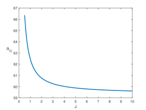
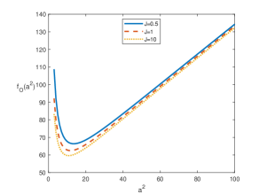
Figure 4: (a): Oscillatory instability threshold as function of the Vadasz term $J$ for $k=10,h=0.1,\mathcal{T}^{2}=10,K_{r}=1.5,\eta=0.2,\gamma=0.8$. (b): Oscillatory thresholds at quoted values of the Vadasz term $J$ and for $k=10,h=0.1,\mathcal{T}^{2}=10,K_{r}=1.5,\eta=0.2,\gamma=0.8$.

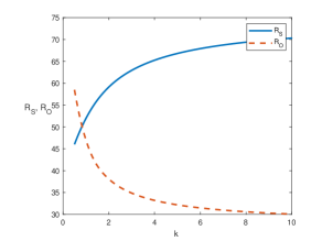
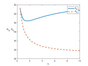
Figure 5: Asymptotic behaviour of the steady and oscillatory instability thresholds as functions of the anisotropic permeability parameters $k$ and $h$. (a): $h=1,\mathcal{T}^{2}=10,J=0.5,K_{r}=1.5,\eta=0.2,\gamma=0.8$. (b): $k=1,\mathcal{T}^{2}=10,J=0.5,K_{r}=1.5,\eta=0.2,\gamma=0.8$.

In figures 1 and 2 the instability thresholds at quoted values of the permeability parameters $h$ and $k$ are shown, for small and large Vadasz term $J$, respectively. From figure 3 we may visualize the stabilizing effect of the Taylor number $\mathcal{T}^{2}$ on the onset of convection, in particular from figure $\ref{FIGURA3}(a)$ two very different growth rates of the steady and of the oscillatory instability thresholds arise. Figure 4 shows the destabilizing effect on the onset of oscillatory convection of the Vadasz coefficient $J$. The numerical results of table 2 are graphically shown in figure 5, where steady and oscillatory instability thresholds are represented as functions of the anisotropic permeability parameters $k$ and $h$.

$R_{S}$	$R_{O}$	$a^{2}_{S}$	$a^{2}_{O}$	$k$
55.5802	$\not\exists$	15.0097	$\not\exists$	0.1
46.4633	$\not\exists$	15.4106	$\not\exists$	0.5
46.7672	$\not\exists$	15.4530	$\not\exists$	0.53
46.8724	48.0833	15.4670	10.8010	0.54
46.9790	47.7998	15.4809	10.7872	0.55
47.0871	47.5233	15.4947	10.7733	0.56
47.1964	47.2537	15.5084	10.7596	0.57
47.3067	46.9906	15.5220	10.7459	0.58
47.5300	46.4833	15.5487	10.7186	0.6
51.9256	39.7591	15.9190	10.2433	1
66.8036	28.7339	15.6424	8.7834	5
70.3183	27.0015	15.3278	8.4389	10

$R_{S}$	$R_{O}$	$a^{2}_{S}$	$a^{2}_{O}$	$h$
146.5652	133.6558	22.0926	10.6720	0.01
88.7111	86.2352	26.9067	14.1899	0.1
56.9286	48.5663	18.8637	11.9393	0.5
51.9256	39.7591	15.9190	10.2433	1
54.1833	31.1656	13.6497	8.3863	5
57.0855	30.0809	13.6502	8.2253	10
61.7553	29.1760	13.8544	8.1706	100

Table 1: Critical steady and oscillatory Rayleigh numbers and wavenumbers for quoted values of $k$ (a) and for quoted values of $h$ (b). Table a: $h=1,\mathcal{T}^{2}=10,J=10,K_{r}=1.5,\eta=0.2,\gamma=0.8$. Table b: $k=1,\mathcal{T}^{2}=10,J=10,K_{r}=1.5,\eta=0.2,\gamma=0.8$.

$R_{S}$	$R_{O}$	$a^{2}_{S}$	$a^{2}_{O}$	$k$
55.5802	$\not\exists$	15.0097	$\not\exists$	0.1
46.4633	$\not\exists$	15.4106	$\not\exists$	0.5
49.8064	$\not\exists$	15.7735	$\not\exists$	0.8
50.0286	$\not\exists$	15.7914	$\not\exists$	0.82
50.1389	50.2184	15.8001	13.4683	0.83
50.2488	49.9896	15.8085	13.4404	0.84
50.3581	49.7655	15.8168	13.4130	0.85
50.8960	48.7116	15.8553	13.2826	0.9
51.9256	46.8876	15.9190	13.0503	1
66.8036	32.1661	15.6424	10.6842	5
70.3183	30.0517	15.3278	10.2302	10

$R_{S}$	$R_{O}$	$a^{2}_{S}$	$a^{2}_{O}$	$h$
88.7111	$\not\exists$	26.9067	$\not\exists$	0.1
59.6059	$\not\exists$	20.0551	$\not\exists$	0.4
58.1248	$\not\exists$	19.4148	$\not\exists$	0.45
57.8653	58.3814	19.2980	15.3814	0.46
57.6164	57.9856	19.1847	15.3599	0.47
57.3777	57.6028	19.0746	15.2905	0.48
57.1486	57.2324	18.9676	15.2227	0.49
56.9286	56.8737	18.8637	15.1563	0.5
51.9256	46.8876	15.9190	13.0503	1
54.1833	36.1050	13.6497	10.4542	5
57.0855	34.4490	13.6502	10.1144	10

Table 2: Critical steady and oscillatory Rayleigh numbers and wavenumbers for quoted values of $k$ (a) and for quoted values of $h$ (b). Table a: $h=1,\mathcal{T}^{2}=10,J=0.5,K_{r}=1.5,\eta=0.2,\gamma=0.8$. Table b: $k=1,\mathcal{T}^{2}=10,J=0.5,K_{r}=1.5,\eta=0.2,\gamma=0.8$.

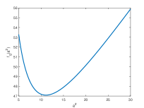
(a) $h>>k$

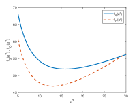
(b) $h=k$

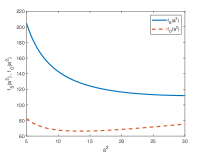
(c) $h<<k$

Figure 1: Instability thresholds for quoted values of $k$ and $h$ and for $\mathcal{T}^{2}=10,{\bf J=0.5},K_{r}=1.5,\eta=0.2,\gamma=0.8$. (a): $h=10,k=0.1$, (b): $h=k=1$, (c): $h=0.1,k=10$.

(a) $h>>k$

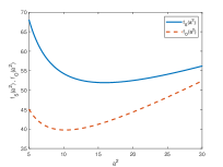
(b) $h=k$

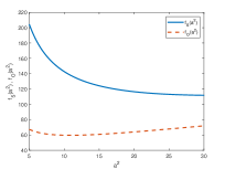
(c) $h<<k$

Figure 2: Instability thresholds for quoted values of $k$ and $h$ and for $\mathcal{T}^{2}=10,{\bf J=10},K_{r}=1.5,\eta=0.2,\gamma=0.8$. (a): $h=10,k=0.1$, (b): $h=k=1$, (c): $h=0.1,k=10$.

$R_{O}$	$a^{2}_{O}$	$J$
$\not\exists$	$\not\exists$	0
$\not\exists$	$\not\exists$	0.1
94.6887	27.8062	0.11
85.6326	23.1078	0.15
66.3568	13.5068	0.5
62.4493	11.8203	1
59.8788	10.9098	5
59.6123	10.8360	10
59.4095	10.7843	50
59.3849	10.7784	100

(a) $h<<k$

$R_{O}$	$a^{2}_{O}$	$J$
$\not\exists$	$\not\exists$	0
$\not\exists$	$\not\exists$	0.5
$\not\exists$	$\not\exists$	1
$\not\exists$	$\not\exists$	5
$\not\exists$	$\not\exists$	10
$\not\exists$	$\not\exists$	50
$\not\exists$	$\not\exists$	100

(b) $h>>k$

Table 3: Critical oscillatory Rayleigh numbers and wavenumbers for quoted values of $J$ for $h<<k$ (a) and for $h>>k$ (b). Table a: for $h=0.1,k=10,\mathcal{T}^{2}=10,K_{r}=1.5,\eta=0.2,\gamma=0.8$ (for these values, critical steady Rayleigh number and wavenumber are $R_{S}=111.7045,a^{2}_{S}=32.4936$). Table b: for $h=10,k=0.1,\mathcal{T}^{2}=10,K_{r}=1.5,\eta=0.2,\gamma=0.8$ (for these values, critical steady Rayleigh number and wavenumber are $R_{S}=47.0944,a^{2}_{S}=11.0770$).

$R_{S}$	$R_{O}$	$a^{2}_{S}$	$a^{2}_{O}$	$\mathcal{T}^{2}$
37.9913	$\not\exists$	8.8113	$\not\exists$	0
61.7538	$\not\exists$	17.9673	$\not\exists$	2
62.5794	$\not\exists$	18.2713	$\not\exists$	2.09
62.6704	64.6393	18.3047	12.2819	2.1
63.5719	64.6626	18.6347	12.2984	2.2
64.4590	64.6858	18.9577	12.3149	2.3
65.3325	64.7090	19.2739	12.3313	2.4
66.1929	64.7321	19.5835	12.3477	2.5
84.6085	65.2968	25.6964	12.7489	5
111.7045	66.3568	32.4936	13.5068	10

(a) $h<<k$

$R_{S}$	$R_{O}$	$a^{2}_{S}$	$a^{2}_{O}$	$\mathcal{T}^{2}$
39.6844	$\not\exists$	8.8024	$\not\exists$	0
43.4949	$\not\exists$	10.0015	$\not\exists$	5
47.0944	$\not\exists$	11.0770	$\not\exists$	10
100.1927	$\not\exists$	22.9601	$\not\exists$	100

(b) $h>>k$

Table 4: Critical steady and oscillatory Rayleigh numbers and wavenumbers for quoted values of $\mathcal{T}^{2}$ for $h<<k$ (a) and for $h>>k$ (b). Table a: for $h=0.1,k=10,J=0.5,K_{r}=1.5,\eta=0.2,\gamma=0.8$. Table b: for $h=10,k=0.1,J=0.5,K_{r}=1.5,\eta=0.2,\gamma=0.8$.

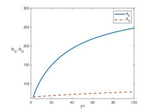
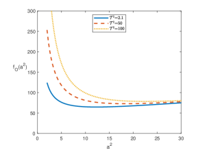
Figure 3: (a): Stationary and Oscillatory instability thresholds as functions of the Taylor number $\mathcal{T}^{2}$ for $k=10,h=0.1,J=0.5,K_{r}=1.5,\eta=0.2,\gamma=0.8$. (b): Oscillatory thresholds at quoted values of the Taylor number $\mathcal{T}^{2}$ and for $k=10,h=0.1,J=0.5,K_{r}=1.5,\eta=0.2,\gamma=0.8$.

5 Conclusions

The onset of convection in a rotating and anisotropic BDPM, taking into account the Vadasz term, has been studied via linear instability analysis. Let us remark that the Vadasz term allows the onset of oscillatory convection, which is not present when the inertia is neglected (see [4]). Moreover, if $h=k=1$, i.e. confining ourselves to the isotropic case, from $(\ref{staz})$ and $(\ref{osc})$ we recover the stationary and oscillatory thresholds found in [5], respectively. Lastly, it has been numerically investigated the relationship between the critical steady and oscillatory Rayleigh numbers and the fundamental parameters $h,k,\mathcal{T}^{2},J$ and we have found out that:

• $R_{S}$ and $R_{O}$ are increasing functions of $\mathcal{T}^{2}$;

• $R_{O}$, if it exists, is a decreasing function of $J$;

• comparing our results with those ones found in [5], anisotropic macropermeability and anisotropic micropermeability lead to higher steady and oscillatory thresholds.

Acknowledgements. This paper has been performed under the auspices of the GNFM of INdAM.

References

- [1] Capone, F., De Luca, R.: Porous MHD Convection: Effect of Vadasz inertia term, Transp. in Porous Media 118(3), pp. 519-536 (2017)
- [2] Capone, F., De Luca, R., Vitiello, M.: Double-diffusive Soret convection phenomenon in porous media: effect of Vadasz inertia term, Ricerche di Matematica 68(2), pp. 581-595 (2019)
- [3] Capone, F., De Luca, R., Gentile, M.: Coriolis effect on thermal convection in a rotating bidisperive porous layer, Proc. R. Soc. A. 47620190875, (2020). https://doi.org/10.1098/rspa.2019.0875
- [4] Capone, F., De Luca, R., Gentile, M.: Thermal convection in rotating anisotropic bidispersive porous layers, Mechanics Research Communications (2020). https://doi.org/10.1016/j.mechrescom.2020.103601
- [5] Capone, F., De Luca, R.: The effect of the Vadasz number on the onset of thermal convection in rotating bidispersive porous media, Fluids 5(4), 173, (2020). https://doi.org/10.3390/fluids5040173
- [6] Capone, F., Gentile, M.: Sharp stability results in LTNE rotating anisotropic porous layer, Int. J. Thermal Sci. 134, pp. 661-664 (2018)
- [7] Capone, F., Gentile, M., Hill, A.A.: Double-diffusive penetrative convection simulated via internal heating in an anisotropic porous layer with throughflow, Int. J. Heat and Mass Transf. 54(7-8), pp. 1622-1626 (2011)
- [8] Chandrasekhar, S.: Hydrodynamic and hydromagnetic stability, Dover Publicationas (1981)
- [9] Gentile, M., Straughan, B.: Bidispersive thermal convection, Int. J. Heat and Mass Transf. 114, pp. 837-840 (2017)
- [10] Gentile, M., Straughan, B.: Bidispersive vertical convection, Proc. R. Soc. A.47320170481 (2017). http://doi.org/10.1098/rspa.2017.0481 J. Fluid Mech., 898 (2020). A14 doi:10.1017/jfm.2020.411
- [11] Kvernvold, O., Tyvand, P.A.: Nonlinear thermal convection in anisotropic porous media, Mechanics and Applied Mathematics 90(4), pp. 609-624 (1977)
- [12] Nield, D.A., Bejan, A.: Convection in Porous Media, 5th edn. New York, NY: Springer (2017)
- [13] Nield, D.A., Kuznetsov, A.V.: A two-velocity temperature model for a bi-dispersed porous medium: forced convection in a channel. Trans. Porous Med. 59, pp. 325–339. (2005)
- [14] Nield, D.A., Kuznetsov, A.V.: Heat transfer in bidisperse porous media, Transport Phenomena in Porous Media III, pp. 34-59 (2005). https://doi.org/10.1016/B978-008044490-1/50006-5
- [15] Nield, D.A., Kuznetsov, A.V.: The onset of convection in a bidisperse porous medium, Int. J. Heat and Mass Transfer, 49(17-18), pp. 3068-3074 (2006)
- [16] Straughan, B.: Convection with Local Thermal Non-equilibrium and Microfluidic Effects, volume 32 of Adv Mechanics and Matematics, Springer, Cham, Switzerland, (2015)
- [17] Straughan, B.: Anisotropic bidispersive convection, Proc. R. Soc. A. 475: 20190206 (2019)
- [18] Straughan, B.: Horizontally isotropic bidispersive thermal convection, Proc. R. Soc. A 474 : 20180018 (2018). http://dx.doi.org/10.1098/rspa.2018.0018
- [19] Straughan, B.: Effect of inertia on double diffusive bidispersive convection, Int. J. Heat and Mass Transfer 129, pp. 389–396 (2019)
- [20] Straughan, B.: Horizontally isotropic double porosity convection, Proc. R. Soc. A. 475: 20180672 (2019)
- [21] Vadasz, P.: Rotating Porous Media, Handbook of porous media (2000)
- [22] Vadasz, P.: Coriolis effect on gravity-driven convection in a rotating porous layer heated from below, J. Fluid Mech., vol. 376, pp. 351-375 (1998)