Stability analysis of reaction-diffusion PDEs coupled at the boundaries with an ODE

Abstract

This paper addresses the derivation of generic and tractable sufficient conditions ensuring the stability of a coupled system composed of a reaction-diffusion partial differential equation (PDE) and a finite-dimensional linear time invariant ordinary differential equation (ODE). The coupling of the PDE with the ODE is located either at the boundaries or in the domain of the reaction-diffusion equation and takes the form of the input and output of the ODE. We investigate boundary Dirichlet/Neumann/Robin couplings, as well as in-domain Dirichlet/Neumann couplings. The adopted approach relies on the spectral reduction of the problem by projecting the trajectory of the PDE into a Hilbert basis composed of the eigenvectors of the underlying Sturm-Liouville operator and yields a set of sufficient stability conditions taking the form of LMIs. We propose numerical examples, consisting of an unstable reaction-diffusion equation and an unstable ODE, such that the application of the derived stability conditions ensure the stability of the resulting coupled PDE-ODE system.

, ,

1 Introduction

The stability analysis and control of coupled PDE-ODE systems has emerged relatively recently in the literature (and more generaly PDEs with dynamical boundary conditions, see e.g. [23]). Such a trend was driven by a certain number of practical applications involving a finite-dimensional dynamics coupled with a phenomenon described by a PDE. This includes, to cite a few, solid–gas interaction of heat diffusion and chemical reaction [31], flexible cranes [15], flexible aircraft [20], drilling mechanisms [5], and power converters connected to transmission lines [12]. PDE-ODE coupling can also arise due to feedback control. Indeed, the PDE can represent the open-loop plant to be controlled while the ODE part gathers controller and actuator dynamics, see e.g. [17, 30]. Conversely, the PDE can represent the dynamics of an actuator (e.g., heat or flux sensors) that is embedded into the closed-loop control of a finite-dimensional plant modeled by an ODE.

The stabilization of PDE-ODE couplings has attracted much attention in the recent years. One of the very first contributions in this field was reported in [17] dealing with the state-feedback stabilization and the observer design of a diffusion PDE cascaded with an ODE via Dirichlet connection (see also [30] for the case of Neumann interconnections). Such a problem can be interpreted as a compensation problem of an infinite-dimensional input dynamics [18] and was solved by employing a backstepping control design procedure. This approach was also reported in the case of string equation in [16, 30] and was later on applied to other types of PDEs such as beam [34] and linearized Korteweg–de Vries [2] equations. This backstepping-based procedure for PDE-ODE cascades was then extended to other boundary stabilization problems such as wave PDEs cascaded with MIMO LTI systems [8], a diffusion PDE coupled with an ODE [31], and a diffusion PDE sandwiched between two ODEs [32]. The robustness of certain of these control strategies for the stabilization of PDE-ODE cascades were studied in [17, 30, 28], particularly for heat equations w.r.t. the diffusion coefficient and the length of the diffusion domain. Other extensions embracing the augmentation of the backstepping transformation with either adaptive or sliding mode control have been investigated in [21, 33]. Recently, a different control design strategy using Sylvester equation was proposed in [22] for ODE-PDE and PDE-ODE cascades.

In this context, the focus of this paper is put on the derivation of generic and tractable sufficient stability conditions ensuring the stability of coupled systems composed of a general reaction-diffusion PDE and an ODE, with various coupling configurations, rather than on the design of a particular controller for a specific setting. The derivation of such analysis tools for stability assessment of PDE-ODE loops is of primary importance. Indeed, such generic stability conditions can be used to assess a posteriori the stability of open-loop unstable reaction-diffusion PDEs when placed in closed-loop with a controller designed empirically using a finite-dimensional truncated model of the PDE. Conversely, considering the infinite-dimensional control strategies reported in the previous paragraph, their practical implementation require their finite-dimensional approximation. In that case, stability analysis tools are required to assess that the finite-dimensional approximation of the controller dynamics still achieves the stabilization of the PDE.

The traditional approach for studying the stability of coupled PDE-ODE systems consists of the adequate selection of a Lyapunov functional. At a very high level, the general trend is to build the Lyapunov functional by considering terms related to 1) the energy of the PDE (measured via a relevant norm); 2) the energy of the ODE; 3) the coupling of the PDE-ODE system. Such Lyapunov functionals can be built manually [10, 11, 19] but can also be obtained numerically by considering very general Lyapunov functional candidates while resorting to numerical methods, such as a sum of square procedure, to obtain an admissible suitable set of parameters [1, 14].

In the abovementioned context, a number of contributions have been reported in the recent years to study the stability of coupled PDE-ODE systems with couplings occurring at the boundaries of the PDE. A first fruitful approach relies on the introduction of a partial integral representation of the PDE [26] in order to study the stability of PDE-ODE loops using linear matrix inequalities (LMIs). Such an approach can be used to study PDE-ODE loops using convex optimization tools [13, 27, 29]. A second fruitful approach relies on the use of Legendre polynomials as a basis of projection for the PDE trajectories. In essence, this consists of the construction of a classical Lyapunov functional accounting for the PDE and ODE parts considered separately while adding a cross quadratic term mixing the state of the ODE with a finite number of coefficients of projection of the PDE trajectory into the basis of Legendre polynomials. Such an approach was reported in [7] for the study of a coupled system composed of a reaction PDE and an ODE. This method was also reported in [6] in the case of a string equation coupled with an ODE, as well as in [3] for the study of input-output stability. Input-output stability properties for coupled PDE-ODE systems using Legendre polynomials-based projections was further investigated in [4]. Finally, the stability of abstract boundary control systems with dynamic boundary conditions and positive underlying $C_{0}$-semigroups was studied in [9].

In this paper, we study the stability of a generic 1-D reaction diffusion equation coupled with a finite-dimensional ODE. The approach adopted in this work differs from the methods described in the previous paragraph because it relies on spectral reduction methods. These spectral reduction methods are used to build a suitable Lyapunov functional candidate and derive a set of tractable LMI conditions ensuring the exponential stability of the coupled PDE-ODE system. Compared to [7], which was concerned with an open-loop stable constant coefficient diffusion PDE with left and right Dirichlet couplings, our approach allows the consideration of generic reaction-diffusion PDEs that are possibly open-loop unstable and with variety of couplings that include Dirichlet, Neumann, and Robin traces. Compared to [13, 27, 29] the approach adopted in this paper allows the coupling of the ODE with the PDE through a Dirichlet/Neumann trace that can be located either at the boundary or inside the spatial domain. Moreover, the exponential stability results derived in this paper are established for system trajectories evaluated in $H^{1}$-norm. This feature has two important implications: 1) the exponential decrease of the PDE trajectories in $L^{\infty}$-norm; and 2) the exponential decay of the coupling channels between ODE and PDE components. This last point is of paramount importance for practical applications because it ensures that the signals in the actuation/sensing channels are also convergent. The relevance of these LMI conditions are assessed based on numerical examples associated with PDEs and ODEs that are all unstable.

The rest of the paper is organized as follows. Section 2 describes the notations and reports a number of basic properties for Sturm-Liouville operators. Then the study is split into two parts. Firstly, the case of a Dirichlet trace used as an input for the ODE is investigated in Section 3. Secondly, the case of a Neumann trace used as an input for the ODE is reported in Section 4. Finally, concluding remarks are formulated in Section 5.

2 Notation and properties

Spaces $\mathbb{R}^{n}$ are endowed with the Euclidean norm denoted by $\|\cdot\|$. The associated induced norms of matrices are also denoted by $\|\cdot\|$. $L^{2}(0,1)$ stands for the space of square integrable functions on $(0,1)$ and is endowed with the inner product $\langle f,g\rangle=\int_{0}^{1}f(x)g(x)\,\mathrm{d}x$ and the norm is denoted by $\|\cdot\|_{L^{2}}$. For an integer $m\geq 1$, the $m$-order Sobolev space is denoted by $H^{m}(0,1)$ and is endowed with its usual norm $\|\cdot\|_{H^{m}}$. For a symmetric matrix $P\in\mathbb{R}^{n\times n}$, $P\succeq 0$ (resp. $P\succ 0$) means that $P$ is positive semi-definite (resp. positive definite) while $\lambda_{M}(P)$ (resp. $\lambda_{m}(P)$) denotes its maximal (resp. minimal) eigenvalue.

Let $\theta_{1},\theta_{2}\in[0,\pi/2]$, $p\in\mathcal{C}^{1}([0,1])$ with $p>0$, and $q\in\mathcal{C}^{0}([0,1])$ with $q\geq 0$. Let the Sturm-Liouville operator $\mathcal{A}:D(\mathcal{A})\subset L^{2}(0,1)\rightarrow L^{2}(0,1)$ be defined by $\mathcal{A}f=-(pf^{\prime})^{\prime}+qf$ on the domain $D(\mathcal{A})=\{f\in H^{2}(0,1)\,:\,\cos(\theta_{1})f(0)-\sin(\theta_{1})f^{\prime}(0)=0,\,\allowbreak\cos(\theta_{2})f(1)+\sin(\theta_{2})f^{\prime}(1)=0\}$. The operator $\mathcal{A}$ is self-adjoint and its eigenvalues $\lambda_{n}$, $n\geq 1$, are simple, non negative, and form an increasing sequence with $\lambda_{n}\rightarrow+\infty$ as $n\rightarrow+\infty$. Moreover, the associated unit eigenvectors $\phi_{n}\in L^{2}(0,1)$ form a Hilbert basis and we also have $D(\mathcal{A})=\{f\in L^{2}(0,1)\,:\,\sum_{n\geq 1}|\lambda_{n}|^{2}|\left<f,\phi_{n}\right>|^{2}<+\infty\}$ with $\mathcal{A}f=\sum_{n\geq 1}\lambda_{n}\left<f,\phi_{n}\right>\phi_{n}$.

Let $p_{*},p^{*},q^{*}\in\mathbb{R}$ be such that $0<p_{*}\leq p(\xi)\leq p^{*}$ and $0\leq q(\xi)\leq q^{*}$ for all $\xi\in[0,1]$, then it holds [24]:

$$0\leq\pi^{2}(n-1)^{2}p_{*}\leq\lambda_{n}\leq\pi^{2}n^{2}p^{*}+q^{*}$$ (1)

for all $n\geq 1$. Assuming further than $p\in\mathcal{C}^{2}([0,1])$, we have for any given $\xi\in[0,1]$ that $\phi_{n}(\xi)=O(1)$ and $\phi_{n}^{\prime}(\xi)=O(\sqrt{\lambda_{n}})$ as $n\rightarrow+\infty$ (see [24]), where $O$ denotes the Bachmann–Landau asymptotic notation. Moreover, we also have, for all $f\in D(\mathcal{A})$, $\left<\mathcal{A}f,f\right>=\sum_{n\geq 1}\lambda_{n}\left<f,\phi_{n}\right>^{2}=\int_{0}^{1}p(f^{\prime})^{2}+qf^{2}\,\mathrm{d}\xi+p(0)f(0)f^{\prime}(0)-p(1)f(1)f^{\prime}(1)$. Hence, provided $q>0$ and because $\theta_{1},\theta_{2}\in[0,\pi/2]$ and $p>0$, we obtain the existence of constants $C_{1},C_{2}>0$ so that

$$C_{1}\|f\|_{H^{1}}^{2}\leq\sum_{n\geq 1}\lambda_{n}\left<f,\phi_{n}\right>^{2}=\left<\mathcal{A}f,f\right>\leq C_{2}\|f\|_{H^{1}}^{2}$$ (2)

for any $f\in D(\mathcal{A})$. This in particular implies that, for any $f\in D(\mathcal{A})$ and any $\xi\in[0,1]$, $f(\xi)=\sum_{n\geq 1}\left<f,\phi_{n}\right>\phi_{n}(\xi)$ and $f^{\prime}(\xi)=\sum_{n\geq 1}\left<f,\phi_{n}\right>\phi_{n}^{\prime}(\xi)$. For any $\alpha\in(0,1)$, we introduce the fractional powers of $\mathcal{A}$ by defining $D(\mathcal{A}^{\alpha})=\{f\in L^{2}(0,1)\,:\,\sum_{n\geq 1}|\lambda_{n}|^{2\alpha}|\left<f,\phi_{n}\right>|^{2}<+\infty\}$ and $\mathcal{A}^{\alpha}f=\sum_{n\geq 1}\lambda_{n}^{\alpha}\left<f,\phi_{n}\right>\phi_{n}$.

For any $f\in L^{2}(0,1)$ we define $\mathcal{P}_{N}f=f-\sum_{n=1}^{N}\left<f,\phi_{n}\right>\phi_{n}=\sum_{n\geq N+1}\left<f,\phi_{n}\right>\phi_{n}$

3 Dirichlet trace as an input of the ODE

3.1 Coupled PDE-ODE systems

We consider in this section the following PDE-ODE system:

$$z_{t}(t,\xi)=(pz_{\xi})_{\xi}(t,\xi)-\tilde{q}(\xi)z(t,\xi)$$ (3a)

$$\cos(\theta_{1})z(t,0)-\sin(\theta_{1})z_{\xi}(t,0)=0$$ (3b)

$$\cos(\theta_{2})z(t,1)+\sin(\theta_{2})z_{\xi}(t,1)=y(t)=Cx(t)$$ (3c)

$$\dot{x}(t)=Ax(t)+Bz(t,\zeta_{m})$$ (3d)

$$z(0,\xi)=z_{0}(\xi),\quad x(0)=x_{0}$$ (3e)

for $t>0$ and $\xi\in(0,1)$ where $\theta_{1},\theta_{2}\in[0,\pi/2]$, $p\in\mathcal{C}^{2}([0,1])$ with $p>0$, $\tilde{q}\in\mathcal{C}^{0}([0,1])$, and $\zeta_{m}\in[0,1]$. Here $A\in\mathbb{R}^{n\times n}$, $B\in\mathbb{R}^{n}$, and $C\in\mathbb{R}^{1\times n}$ are matrices, $z_{0}\in L^{2}(0,1)$ and $x_{0}\in\mathbb{R}^{n}$ are initial conditions, and $z(t,\cdot)\in L^{2}(0,1)$ and $x(t)\in\mathbb{R}^{n}$ are the state of the reaction-diffusion PDE and of the ODE at time $t$, respectively.

The PDE-ODE system (3) consists of a reaction-diffusion PDE coupled with an ODE. The output $y(t)=Cx(t)$ of the ODE is seen as a boundary input for the PDE and is applied at the right Robin boundary condition. Conversely, the pointwise Dirichlet trace $z(t,\zeta_{m})$ is seen as an input of the ODE (3d). The objective of this section is to derive numerically tractable sufficient conditions ensuring the exponential stability of the PDE-ODE system (3) when evaluating the PDE trajectory in $H^{1}$-norm.

We introduce without loss of generality $q\in\mathcal{C}^{0}([0,1])$ and $q_{c}\in\mathbb{R}$ such that

$$\tilde{q}=q-q_{c},\quad q>0.$$ (4)

Remark 1.

Even if the presentation focuses on the case $\theta_{1},\theta_{2}\in[0,\pi/2]$, the derived results can be extended to $\theta_{1},\theta_{2}\in[0,2\pi]$. Indeed, considering first the case $\theta_{1},\theta_{2}\in[0,\pi]$, the proposed strategy also applies provided 1) $q>0$ from (4) is selected large enough so that the estimates (2) still hold for some constants $C_{1},C_{2}>0$; 2) the change of variable (5) is replaced by $w(t,\xi)=z(t,\xi)-\frac{\xi^{\alpha}}{\cos\theta_{2}+\alpha\sin\theta_{2}}y(t)$ for any fixed $\alpha>1$ selected so that $\cos(\theta_{2})+\alpha\cos(\theta_{2})\neq 0$. Finally, in view of (3b-3c), the general case $\theta_{1},\theta_{2}\in[0,2\pi]$ reduces to the case $\theta_{1},\theta_{2}\in[0,\pi]$ by proceeding with the following substitutions: 1) if $\theta_{1}\in(\pi,2\pi]$ then $\theta_{1}\leftarrow\theta_{1}-\pi$; 2) if $\theta_{2}\in(\pi,2\pi]$ then $\theta_{2}\leftarrow\theta_{2}-\pi$ and $C\leftarrow-C$.

Remark 2.

System (3), as well as system (15) that will be described in the next section, can be used to represent a variety of practical situations. For instance the PDE part can stand for a reaction-diffusion process coupled with a finite-dimensional LTI controller materialized by the ODE. Conversely, the ODE part can merge both finite-dimensional LTI plant along with its associated finite-dimensional LTI controller while the PDE part describes the sensor dynamics. This latter situation is similar to the one described in [17] where a controller was designed for a cascaded PDE-ODE system using a backstepping transformation. One of the main motivations for deriving generic stability conditions for coupled PDE-ODE systems such as (3) is ultimately when the to-be-implemented finite-dimensional controller is computed either on a finite-dimensional approximation of the PDE or via the approximation of an infinite-dimensional output feedback controller (obtained, e.g., using backstepping control design procedures).

Remark 3.

The PDE-ODE system (3) with $\theta_{1}=\pi/2$, $\theta_{2}=0$, and $\zeta_{m}=0$ was studied in [7] in the case of a stable diffusion PDE (i.e., without reaction term) and with a constant diffusion coefficient using the projection of the PDE trajectories into a finite subset of Legendre polynomials.

3.2 Preliminary spectral reduction

We rewrite (3) under an equivalent PDE-ODE system with homogeneous boundary conditions. Specifically, introducing the change of variable

$$w(t,\xi)=z(t,\xi)-\frac{\xi^{2}}{\cos\theta_{2}+2\sin\theta_{2}}y(t)$$ (5)

we infer that (3) is equivalent to

$$w_{t}(t,\xi)=(pw_{\xi})_{\xi}(t,\xi)+(q_{c}-q(\xi))w(t,\xi)$$ (6a)

$$\phantom{w_{t}(t,\xi)=}\;+a(\xi)y(t)+b(\xi)\dot{y}(t)$$

$$\cos(\theta_{1})w(t,0)-\sin(\theta_{1})w_{\xi}(t,0)=0$$ (6b)

$$\cos(\theta_{2})w(t,1)+\sin(\theta_{2})w_{\xi}(t,1)=0$$ (6c)

$$y(t)=Cx(t)$$ (6d)

$$\dot{x}(t)=Ax(t)+B\left(w(t,\zeta_{m}\right)+\mu_{m}y(t))$$ (6e)

$$w(0,\xi)=w_{0}(\xi),\quad x(0)=x_{0}$$ (6f)

with $a(\xi)=\frac{1}{\cos\theta_{2}+2\sin\theta_{2}}\{2p(\xi)+2\xi p^{\prime}(\xi)+(q_{c}-q(\xi))\xi^{2}\}$, $b(\xi)=-\frac{\xi^{2}}{\cos\theta_{2}+2\sin\theta_{2}}$, $\mu_{m}=-b(\zeta_{m})$, and $w_{0}(\xi)=z_{0}(\xi)-\frac{\xi^{2}}{\cos\theta_{2}+2\sin\theta_{2}}y(0)$.

After this change of variable, the well-posedness in terms of classical solutions of the above PDE-ODE system for initial conditions $w_{0}\in D(\mathcal{A}^{1/2})$ and $x_{0}\in\mathbb{R}^{n}$ is a consequence of [25, Thm. 6.3.1 and 6.3.3]. More precisely, we have for any $w_{0}\in D(\mathcal{A}^{1/2})$ and any $x_{0}\in\mathbb{R}^{n}$ the existence and uniqueness of a classical solution $(w,x)\in\mathcal{C}^{0}([0,\infty);L^{2}(0,1)\times\mathbb{R}^{n})\cap\mathcal{C}^{1}((0,\infty);L^{2}(0,1)\times\mathbb{R}^{n})$ with $w(t,\cdot)\in D(\mathcal{A})$ for all $t>0$. Moreover, from the proof of  [25, Thm. 6.3.1], we have $\mathcal{A}w\in\mathcal{C}^{0}((0,\infty);L^{2}(0,1))$ and $\mathcal{A}^{1/2}w\in\mathcal{C}^{0}([0,\infty);L^{2}(0,1))$.

We now introduce the Hilbert basis $\{\phi_{i}\,:\,i\geq 1\}$ of $L^{2}(0,1)$ formed by the eigenvectors of the Sturm-Liouville operator $\mathcal{A}$. We introduce the coefficients of projection:

$$w_{i}(t)=\left<w(t,\cdot),\phi_{i}\right>,\quad a_{i}=\left<a,\phi_{i}\right>,\quad b_{i}=\left<b,\phi_{i}\right>$$ (7)

and define $c_{i}=\phi_{i}(\zeta_{m})$ for $i\geq 1$. Considering classical solutions, we obtain that

$$\dot{w}_{i}(t)=(-\lambda_{i}+q_{c})w_{i}(t)+a_{i}Cx(t)$$ (8a)

$$\phantom{\dot{w}_{i}(t)=}\;+b_{i}C\left\{(A+\mu_{m}BC)x(t)+B\sum_{j\geq 1}c_{j}w_{j}(t)\right\}$$

$$\dot{x}(t)=(A+\mu_{m}BC)x(t)+B\sum_{j\geq 1}c_{j}w_{j}(t)$$ (8b)

for $i\geq 1$. The adopted stability analysis procedure relies now on the introduction of a finite dimensional model that captures the dynamics of the ODE (8b) along with the $N\geq 1$ first modes $w_{i}$ of the PDE plant, described by (8a), while bounding the effect of the residue of measurement $\mathcal{R}(t)=\sum_{i\geq N+1}c_{i}w_{i}(t)$ by using Lyapunov’s direct method. To do so, we define

$$W(t) =\begin{bmatrix}w_{1}(t)&\ldots&w_{N}(t)\end{bmatrix}^{\top}\in\mathbb{R}^{N},$$

$$A_{N} =\mathrm{diag}(-\lambda_{1}+q_{c},\ldots,-\lambda_{N}+q_{c})\in\mathbb{R}^{N\times N},$$

$$B_{a,N} =\begin{bmatrix}a_{1}&\ldots&a_{N}\end{bmatrix}^{\top}\in\mathbb{R}^{N},$$

$$B_{b,N} =\begin{bmatrix}b_{1}&\ldots&b_{N}\end{bmatrix}^{\top}\in\mathbb{R}^{N},$$

$$C_{N} =\begin{bmatrix}c_{1}&\ldots&c_{N}\end{bmatrix}\in\mathbb{R}^{1\times N}.$$

We infer from (8a) that

$$\dot{W}(t) =(A_{N}+B_{b,N}CBC_{N})W(t)+B_{b,N}CB\mathcal{R}(t)$$

$$\phantom{=}\;+(B_{a,N}C+B_{b,N}C(A+\mu_{m}BC))x(t).$$

Combining this latter identity with (8b) while defining

$$X(t)=\begin{bmatrix}W(t)\\ x(t)\end{bmatrix}\in\mathbb{R}^{N+n},$$

we infer that

$$\dot{X}(t)=FX(t)+G\mathcal{R}(t)$$ (9)

where

$$F=\begin{bmatrix}A_{N}+B_{b,N}CBC_{N}&B_{a,N}C+B_{b,N}C(A+\mu_{m}BC)\\ BC_{N}&A+\mu_{m}BC\end{bmatrix}$$

and

$$G=\begin{bmatrix}B_{b,N}CB\\ B\end{bmatrix}.$$

Hence, the ODE (9) describes the dynamics of the ODE and of the $N$ first modes $w_{i}$ of the PDE plant while taking as an input the residue of measurement $\mathcal{R}(t)=\sum_{i\geq N+1}c_{i}w_{i}(t)$. The residual dynamics, which corresponds to the modes $i\geq N+1$, is characterized by

$$\dot{w}_{i}(t) =(-\lambda_{i}+q_{c})w_{i}(t)+a_{i}Cx(t)+b_{i}C(A+\mu_{m}BC)x(t)$$

$$\phantom{=}\;+b_{i}CBC_{N}W(t)+b_{i}CB\mathcal{R}(t).$$ (10)

In preparation of the stability analysis, we introduce the matrix

$$H=\begin{bmatrix}H_{1,1}&0\\ 0&H_{2,2}\end{bmatrix}$$

with $H_{1,1}=\|\mathcal{P}_{N}b\|_{L^{2}}^{2}C_{N}^{\top}B^{\top}C^{\top}CBC_{N}$ and $H_{2,2}=\|\mathcal{P}_{N}a\|_{L^{2}}^{2}C^{\top}C+\|\mathcal{P}_{N}b\|_{L^{2}}^{2}(A+\mu_{m}BC)^{\top}C^{\top}C(A+\mu_{m}BC)$. We finally define the constant defined by $M_{1,\phi}=\sum_{i\geq N+1}\frac{\phi_{i}(\zeta_{m})^{2}}{\lambda_{i}}$ which is finite because (1) along with $\phi_{n}(\zeta_{m})=O(1)$ as $n\rightarrow+\infty$.

3.3 Main result

We can now introduce the main result of this section.

Theorem 4.

Let $\theta_{1},\theta_{2}\in[0,\pi/2]$, $p\in\mathcal{C}^{2}([0,1])$ with $p>0$, $\tilde{q}\in\mathcal{C}^{0}([0,1])$, $\zeta_{m}\in[0,1]$, $A\in\mathbb{R}^{n\times n}$, $B\in\mathbb{R}^{n}$, and $C\in\mathbb{R}^{1\times n}$ be given. Let $q\in\mathcal{C}^{0}([0,1])$ and $q_{c}\in\mathbb{R}$ be such that (4) holds. Assume that there exist $N\geq 1$, $P\succ 0$, $\alpha>2$, and $\beta>0$ such that $\Theta_{1}\prec 0$ and $\Theta_{2}\prec 0$ where

$$\Theta_{1} =\begin{bmatrix}F^{\top}P+PF+\alpha H&PG\\ G^{\top}P&\alpha\|\mathcal{P}_{N}b\|_{L^{2}}^{2}(CB)^{2}-\beta\end{bmatrix},$$

$$\Theta_{2} =\begin{bmatrix}-\lambda_{N+1}+q_{c}+\frac{\beta M_{1,\phi}}{2}&\sqrt{2\lambda_{N+1}}\\ \sqrt{2\lambda_{N+1}}&-\alpha\end{bmatrix}.$$

Then there exist constants $\eta,M>0$ such that, for any initial conditions $z_{0}\in H^{2}(0,1)$ and $x_{0}\in\mathbb{R}^{n}$ such that $\cos(\theta_{1})z_{0}(0)-\sin(\theta_{1})z_{0}^{\prime}(0)=0$ and $\cos(\theta_{2})z_{0}(1)+\sin(\theta_{2})z_{0}^{\prime}(1)=Cx_{0}$, the classical solution of (3) satisfies

$$\|z(t,\cdot)\|_{H^{1}}^{2}+\|x(t)\|^{2}\leq Me^{-2\eta t}(\|z_{0}\|_{H^{1}}^{2}+\|x_{0}\|^{2})$$ (11a)

with coupling channels such that

$$z(t,\zeta_{m})^{2}+y(t)^{2}\leq Me^{-2\eta t}(\|z_{0}\|_{H^{1}}^{2}+\|x_{0}\|^{2})$$ (11b)

for all $t>0$.

Remark 5.

The conclusions of Theorem 4 actually hold for any initial conditions such that $w_{0}\in D(\mathcal{A}^{1/2})$. For example the case $\theta_{1}=\pi/2$ and $\theta_{2}=0$ leads to $D(\mathcal{A}^{1/2})=\left\{f\in H^{1}(0,1)\,:\,f(1)=0\right\}$. In this setting the conclusions of Theorem 4 hold for any $z_{0}\in H^{1}(0,1)$ and $x_{0}\in\mathbb{R}^{n}$ such that $z_{0}(1)=Cx_{0}$. Similarly, the case $\theta_{1}=\theta_{2}=\pi/2$ gives $D(\mathcal{A}^{1/2})=H^{1}(0,1)$, implying that the conclusions of Theorem 4 hold for any $z_{0}\in H^{1}(0,1)$ and $x_{0}\in\mathbb{R}^{n}$.

Proof. Let $N\geq 1$, $P\succ 0$, $\alpha>2$, and $\beta>0$ such that $\Theta_{1}\prec 0$ and $\Theta_{2}\prec 0$. Hence, there exist $\eta>0$ such that $\Theta_{1,\eta}\preceq 0$ and $\Theta_{2,\eta}\preceq 0$ where

$$\Theta_{1,\eta} =\begin{bmatrix}F^{\top}P+PF+2\eta P+\alpha H&PG\\ G^{\top}P&\alpha\|\mathcal{P}_{N}b\|_{L^{2}}^{2}(CB)^{2}-\beta\end{bmatrix},$$

$$\Theta_{2,\eta} =\begin{bmatrix}-\lambda_{N+1}+q_{c}+\eta+\frac{\beta M_{1,\phi}}{2}&\sqrt{2\lambda_{N+1}}\\ \sqrt{2\lambda_{N+1}}&-\alpha\end{bmatrix}.$$

Define the Lyapunov functionnal candidate

$$V(X,w)=X^{\top}PX+\sum_{i\geq N+1}\lambda_{i}\left<w,\phi_{i}\right>^{2}$$ (12)

with $X\in\mathbb{R}^{N+n}$ and $w\in D(\mathcal{A})$. The first term of the above functional accounts for the finite-dimensional truncated model (9) while the series is used to study the stability of the residual dynamics described by (10) and to bound the effect of the residue of measurement $\mathcal{R}(t)=\sum_{i\geq N+1}c_{i}w_{i}(t)$ which is acting as an input of (9). With the slight abuse of notation $V(t)=V(X(t),w(t))$, the computation of the time derivative of $V$ along the system trajectories (9) and (10) gives for $t>0$

$$\dot{V}(t)=2X(t)^{\top}P\dot{X}(t)+2\sum_{i\geq N+1}\lambda_{i}w_{i}(t)\dot{w}_{i}(t)$$

$$=X(t)^{\top}(F^{\top}P+PF)X(t)+2X(t)^{\top}PG\mathcal{R}(t)$$

$$\phantom{=}\;+2\sum_{i\geq N+1}\lambda_{i}(-\lambda_{i}+q_{c})w_{i}(t)^{2}$$

$$\phantom{=}\;+2\sum_{i\geq N+1}\lambda_{i}w_{i}(t)a_{i}Cx(t)$$

$$\phantom{=}\;+2\sum_{i\geq N+1}\lambda_{i}w_{i}(t)b_{i}C(A+\mu_{m}BC)x(t)$$

$$\phantom{=}\;+2\sum_{i\geq N+1}\lambda_{i}w_{i}(t)b_{i}CBC_{N}W(t)$$

$$\phantom{=}\;+2\sum_{i\geq N+1}\lambda_{i}w_{i}(t)b_{i}CB\mathcal{R}(t).$$

We estimate the four latter series by using Young’s inequality. For instance, the first term is estimated as

$$2\sum_{i\geq N+1}\lambda_{i}w_{i}(t)a_{i}Cx(t)$$

$$\leq\sum_{i\geq N+1}\left\{\frac{1}{\alpha}\lambda_{i}^{2}w_{i}(t)^{2}+\alpha a_{i}^{2}(Cx(t))^{2}\right\}$$

$$\leq\frac{1}{\alpha}\sum_{i\geq N+1}\lambda_{i}^{2}w_{i}(t)^{2}+\alpha\|\mathcal{P}_{N}a\|_{L^{2}}^{2}x(t)^{\top}C^{\top}Cx(t).$$

Similarly, we obtain that

$$2\sum_{i\geq N+1}\lambda_{i}w_{i}(t)b_{i}C(A+\mu_{m}BC)x(t)\leq\frac{1}{\alpha}\sum_{i\geq N+1}\lambda_{i}^{2}w_{i}(t)^{2}$$

$$+\alpha\|\mathcal{P}_{N}b\|_{L^{2}}^{2}x(t)^{\top}(A+\mu_{m}BC)^{\top}C^{\top}C(A+\mu_{m}BC)x(t),$$

$$2\sum_{i\geq N+1}\lambda_{i}w_{i}(t)b_{i}CBC_{N}W(t)\leq\frac{1}{\alpha}\sum_{i\geq N+1}\lambda_{i}^{2}w_{i}(t)^{2}$$

$$+\alpha\|\mathcal{P}_{N}b\|_{L^{2}}^{2}W(t)^{\top}C_{N}^{\top}B^{\top}C^{\top}CBC_{N}W(t),$$

and

$$2\sum_{i\geq N+1}\lambda_{i}w_{i}(t)b_{i}CB\mathcal{R}(t)$$

$$\leq\frac{1}{\alpha}\sum_{i\geq N+1}\lambda_{i}^{2}w_{i}(t)^{2}+\alpha\|\mathcal{P}_{N}b\|_{L^{2}}^{2}(CB)^{2}\mathcal{R}(t)^{2}.$$

The use of the four latter estimates implies that

$$\dot{V}(t)\leq$$

$$\begin{bmatrix}X(t)\\ \mathcal{R}(t)\end{bmatrix}^{\top}\begin{bmatrix}F^{\top}P+PF+\alpha H&PG\\ G^{\top}P&\alpha\|\mathcal{P}_{N}b\|_{L^{2}}^{2}(CB)^{2}\end{bmatrix}\begin{bmatrix}X(t)\\ \mathcal{R}(t)\end{bmatrix}$$

$$+2\sum_{i\geq N+1}\lambda_{i}\left(-\lambda_{i}+q_{c}+\frac{2\lambda_{i}}{\alpha}\right)w_{i}(t)^{2}$$ (13)

for $t>0$. Since $\mathcal{R}(t)=\sum_{i\geq N+1}c_{i}w_{i}(t)$ with $c_{i}=\phi_{i}({\zeta_{m}})$, we infer that $\mathcal{R}(t)^{2}\leq M_{1,\phi}\sum_{i\geq N+1}\lambda_{i}w_{i}(t)^{2}$. This implies for $t>0$ that

$$\dot{V}(t)+2\eta V(t)$$ (14)

$$\leq\begin{bmatrix}X(t)\\ \mathcal{R}(t)\end{bmatrix}^{\top}\Theta_{1,\eta}\begin{bmatrix}X(t)\\ \mathcal{R}(t)\end{bmatrix}+2\sum_{i\geq N+1}\lambda_{i}\Gamma_{i}w_{i}(t)^{2}$$

where $\Gamma_{i}=-\left(1-\frac{2}{\alpha}\right)\lambda_{i}+q_{c}+\eta+\frac{\beta M_{1,\phi}}{2}$. Now, since $\alpha>2$, we have $\Gamma_{i}\leq\Gamma_{N+1}$ for all $i\geq N+1$. Moreover, combining $\Theta_{2,\eta}\preceq 0$ and the Schur complement, we infer that $\Gamma_{N+1}\leq 0$. Using also $\Theta_{1,\eta}\preceq 0$, we obtain that $\dot{V}(t)+2\eta V(t)\leq 0$ for all $t>0$. Since $\mathcal{A}^{1/2}w\in\mathcal{C}^{0}([0,\infty);L^{2}(0,1))$, the mapping $t\mapsto V(t)$ is continuous for $t\geq 0$, implying that $V(t)\leq e^{-2\eta t}V(0)$ for all $t\geq 0$. We now note from (12) that $V(0)\leq\lambda_{M}(P)\|X(0)\|^{2}+\sum_{i\geq N+1}\lambda_{i}\left<w_{0},\phi_{i}\right>^{2}$. Noting that $\|X(0)\|^{2}\leq\|x_{0}\|^{2}+\|w_{0}\|_{L^{2}}^{2}$ and using (2), we infer the existence of a constant $M_{1}>0$ such that $V(0)\leq M_{1}\left(\|x_{0}\|^{2}+\|w_{0}\|_{H^{1}}^{2}\right)$. Using now (2) and (12), we have the existence of a constant $M_{2}>0$ such that $\|w(t,\cdot)\|_{H^{1}}^{2}\leq M_{2}V(t)$. Hence, we infer the existence of a constant $M_{3}>0$ such that $\|w(t,\cdot)\|_{H^{1}}^{2}+\|x(t)\|^{2}\leq M_{3}e^{-2\eta t}\left(\|w_{0}\|_{H^{1}}^{2}+\|x_{0}\|^{2}\right)$. The claimed conclusion follows from the change of variable (5) and the continuous embedding $H^{1}(0,1)\subset L^{\infty}([0,1])$. ∎

From the above proof we deduce the following corollary.

Corollary 6.

In the context of Theorem 4, the decay rate $\eta>0$ of the stability estimate (11) is guaranteed provided the LMI conditions $\Theta_{1,\eta}\preceq 0$ and $\Theta_{2,\eta}\preceq 0$ are feasible.

Remark 7.

For a given order $N$, the implementation of the conditions $\Theta_{1}\prec 0$ and $\Theta_{2}\prec 0$ from Theorem 4 require the computation of the eigenstructures $\lambda_{n}$ and $\phi_{n}$ for $1\leq n\leq N$ as well as (an upper estimate of) $M_{1,\phi}=\sum_{i\geq N+1}\frac{\phi_{i}(\zeta_{m})^{2}}{\lambda_{i}}$. In the case that the eigenstructures cannot be computed analytically, numerical methods can be used to estimate the $N$ first eigenstructures. Moreover, an upper bound of $M_{1,\phi}=\sum_{i\geq N+1}\frac{\phi_{i}(\zeta_{m})^{2}}{\lambda_{i}}$ can be obtained using (1) and by computing an upper bound of $\sup_{n\geq N+1}\max_{x\in[0,1]}\phi_{n}(x)$ by proceeding as in [24].

3.4 Numerical illustration

We illustrate the results of Theorem 4 and Corollary 6 for the coupled PDE-ODE system described by (3) with $\theta_{1}=\pi/2$, $\theta_{2}=0$, $p=1$, $\tilde{q}=-3$, $\zeta_{m}=1/4$,

$$A =\begin{bmatrix}0&-1/4&-1/5&1/5&1/6\\ 1/2&1&-4&9/2&7/2\\ -9/4&-1/2&-14&23&16\\ -1/5&-1/2&-11/4&1/10&5/4\\ -4/3&-4/3&-9&9&5/2\end{bmatrix},$$

$$B =\begin{bmatrix}-7/2&-3/2&-1/10&1/2&1\end{bmatrix}^{\top},$$

$$C =\begin{bmatrix}-1/10&-1/3&-4&7/8&7/8\end{bmatrix}.$$

In this case, both PDE and ODE systems are open-loop unstable. Indeed, the dominant eigenvalue of the PDE is located approximately at $+0.533$ while the matrix $A$ has two unstable eigenvalues located approximately at $+1.046$ and $+0.247$.

We select $q=1$ and $q_{c}=4$ which satisfy (4). Hence, we obtain that $\lambda_{n}=p(n-1/2)^{2}\pi^{2}+q$ and $\phi_{n}(\xi)=\sqrt{2}\cos((n-1/2)\pi\xi)$. Using the integral test for convergence, we infer that $M_{1,\phi}\leq\frac{2}{p\pi^{2}(N-1/2)}$. The application of Theorem 4 with $N=3$ shows the exponential stability of the coupled PDE-ODE system (3). Moreover, the application of Corollary 6 with $N=9$ shows the exponential stability of the coupled PDE-ODE system with decay rate $\eta=0.5$. We illustrate this result with a numerical simulation. The numerical scheme consists in the modal approximation of the PDE plant by its 100 dominant modes. The initial condition is set as $w_{0}(\xi)=-1+\xi^{2}$ and $x_{0}=\begin{bmatrix}-2&1&2&1&3\end{bmatrix}^{\top}$. The obtained results are depicted on Fig. 1, confirming the theoretical predictions of Theorem 4 and Corollary 6.

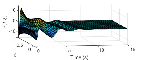
(a) State of the reaction-diffusion system $z(t,\xi)$

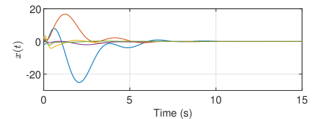
(b) State of the ODE $x(t)$

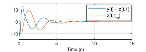
(c) Coupling channels

Figure 1: Time evolution of the coupled PDE-ODE system (3)

4 Neumann trace as an input of the ODE

4.1 Coupled PDE-ODE systems

We consider in this section the case of a reaction-diffusion PDE entering into the ODE by means of a Neumann trace instead of a Dirichlet trace.

$$z_{t}(t,\xi)=(pz_{\xi})_{\xi}(t,\xi)-\tilde{q}(\xi)z(t,\xi)$$ (15a)

$$\cos(\theta_{1})z(t,0)-\sin(\theta_{1})z_{\xi}(t,0)=0$$ (15b)

$$\cos(\theta_{2})z(t,1)+\sin(\theta_{2})z_{\xi}(t,1)=y(t)=Cx(t)$$ (15c)

$$\dot{x}(t)=Ax(t)+Bz_{\xi}(t,\zeta_{m})$$ (15d)

$$z(0,\xi)=z_{0}(\xi),\quad x(0)=x_{0}$$ (15e)

for $t>0$ and $\xi\in(0,1)$ where $\theta_{1},\theta_{2}\in[0,\pi/2]$, $p\in\mathcal{C}^{2}([0,1])$ with $p>0$, $\tilde{q}\in\mathcal{C}^{0}([0,1])$, and $\zeta_{m}\in[0,1]$. Here $A\in\mathbb{R}^{n\times n}$, $B\in\mathbb{R}^{n}$, and $C\in\mathbb{R}^{1\times n}$ are matrices, $z_{0}\in L^{2}(0,1)$ and $x_{0}\in\mathbb{R}^{n}$ are initial conditions, and $z(t,\cdot)\in L^{2}(0,1)$ and $x(t)\in\mathbb{R}^{n}$ are the state of the reaction-diffusion PDE and of the ODE at time $t$, respectively.

Comparing to the PDE-ODE system (3) studied in the previous section, the PDE-ODE system (15) differs by the fact that the input of the ODE (15d) is now the pointwise Neumann trace $z_{\xi}(t,\zeta_{m})$. In this context, the objective of this section is also to derive sufficient conditions ensuring the exponential stability of the PDE-ODE system (15) when evaluating the PDE trajectory in $H^{1}$-norm.

As in the previous section, we introduce without loss of generality a function $q\in\mathcal{C}^{0}([0,1])$ and a constant $q_{c}\in\mathbb{R}$ such that (4) holds.

4.2 Preliminary spectral reduction

Considering the change of variable (5), we infer that (15) is equivalent to

$$w_{t}(t,\xi)=(pw_{\xi})_{\xi}(t,\xi)+(q_{c}-q(\xi))w(t,\xi)$$ (16a)

$$\phantom{w_{t}(t,\xi)=}\;+a(\xi)y(t)+b(\xi)\dot{y}(t)$$

$$\cos(\theta_{1})w(t,0)-\sin(\theta_{1})w_{\xi}(t,0)=0$$ (16b)

$$\cos(\theta_{2})w(t,1)+\sin(\theta_{2})w_{\xi}(t,1)=0$$ (16c)

$$y(t)=Cx(t)$$ (16d)

$$\dot{x}(t)=Ax(t)+B\left(w_{\xi}(t,\zeta_{m})+\mu_{m}y(t)\right)$$ (16e)

$$w(0,\xi)=w_{0}(\xi),\quad x(0)=x_{0}$$ (16f)

where $a$, $b$, and $w_{0}$ are defined as in the previous section while $\mu_{m}=-b^{\prime}(\zeta_{m})$. Note that, after this change of variable, the well-posedness in terms of classical solutions of the above PDE-ODE systems for initial conditions $w_{0}\in\cup_{\alpha_{0}\in(3/4,1)}D(\mathcal{A}^{\alpha_{0}})$ and $x_{0}\in\mathbb{R}^{n}$ is a consequence of [25, Thm. 6.3.1 and 6.3.3]. More precisely, for a given $\alpha_{0}\in(3/4,1)$, we have for any $w_{0}\in D(\mathcal{A}^{\alpha_{0}})$ and any $x_{0}\in\mathbb{R}^{n}$ the existence and uniqueness of a classical solution $(w,x)\in\mathcal{C}^{0}([0,\infty);L^{2}(0,1)\times\mathbb{R}^{n})\cap\mathcal{C}^{1}((0,\infty);L^{2}(0,1)\times\mathbb{R}^{n})$ with $w(t,\cdot)\in D(\mathcal{A})$ for all $t>0$. Moreover, from the proof of  [25, Thm. 6.3.1], we have $\mathcal{A}w\in\mathcal{C}^{0}((0,\infty);L^{2}(0,1))$ and $\mathcal{A}^{\alpha_{0}}w\in\mathcal{C}^{0}([0,\infty);L^{2}(0,1))$ hence $\mathcal{A}^{1/2}w\in\mathcal{C}^{0}([0,\infty);L^{2}(0,1))$.

Proceeding now as in the previous section while replacing the definition of $c_{i}$ by $c_{i}=\phi^{\prime}_{i}(\zeta_{m})$ for all $i\geq 1$, we infer that the truncated model (9) holds while the residual dynamics is described by (10).

We finally define for any $\epsilon\in(0,1/2]$ the constant $M_{2,\phi}(\epsilon)=\sum_{i\geq N+1}\frac{\phi_{i}^{\prime}(\zeta_{m})^{2}}{\lambda_{i}^{3/2+\epsilon}}$ which is finite because (1) along with $\phi^{\prime}_{n}(\zeta_{m})=O(\sqrt{\lambda_{n}})$ as $n\rightarrow+\infty$.

4.3 Main result

We can now introduce the main result of this section.

Theorem 8.

Let $\theta_{1},\theta_{2}\in[0,\pi/2]$, $p\in\mathcal{C}^{2}([0,1])$ with $p>0$, $\tilde{q}\in\mathcal{C}^{0}([0,1])$, $\zeta_{m}\in[0,1]$, $A\in\mathbb{R}^{n\times n}$, $B\in\mathbb{R}^{n}$, and $C\in\mathbb{R}^{1\times n}$ be given. Let $q\in\mathcal{C}^{0}([0,1])$ and $q_{c}\in\mathbb{R}$ be such that (4) holds. Assume that there exist $N\geq 1$, $\epsilon\in(0,1/2]$, $P\succ 0$, $\alpha>2$, and $\beta>0$ such that $\Theta_{1}\prec 0$, $\Theta_{2}\prec 0$, and $\Theta_{3}\succ 0$ where

$$\Theta_{1} =\begin{bmatrix}F^{\top}P+PF+\alpha H&PG\\ G^{\top}P&\alpha\|\mathcal{P}_{N}b\|_{L^{2}}^{2}(CB)^{2}-\beta\end{bmatrix},$$

$$\Theta_{2} =\begin{bmatrix}-\lambda_{N+1}+q_{c}+\frac{\beta M_{2,\phi}(\epsilon)}{2}\lambda_{N+1}^{1/2+\epsilon}&\sqrt{2\lambda_{N+1}}\\ \sqrt{2\lambda_{N+1}}&-\alpha\end{bmatrix},$$

$$\Theta_{3} =\begin{bmatrix}1-\frac{\beta M_{2,\phi}(\epsilon)}{2\lambda_{N+1}^{1/2-\epsilon}}&\sqrt{2}\\ \sqrt{2}&\alpha\end{bmatrix}.$$

Then there exist constants $\eta,M>0$ such that, for any initial conditions $z_{0}\in H^{2}(0,1)$ and $x_{0}\in\mathbb{R}^{n}$ such that $\cos(\theta_{1})z_{0}(0)-\sin(\theta_{1})z_{0}^{\prime}(0)=0$ and $\cos(\theta_{2})z_{0}(1)+\sin(\theta_{2})z_{0}^{\prime}(1)=Cx_{0}$, the classical solution of (15) satisfies

$$\|z(t,\cdot)\|_{H^{1}}^{2}+\|x(t)\|^{2}\leq Me^{-2\eta t}(\|z_{0}\|_{H^{1}}^{2}+\|x_{0}\|^{2})$$ (17a)

with coupling channels such that

$$z_{\xi}(t,\zeta_{m})^{2}+y(t)^{2}\leq Me^{-2\eta t}(\|z_{0}\|_{H^{1}}^{2}+\|\mathcal{A}w_{0}\|_{L^{2}}^{2}+\|x_{0}\|^{2})$$ (17b)

for all $t>0$.

Remark 9.

For any fixed $\alpha_{0}\in(3/4,1)$, the estimate (17a) of Theorem 8 actually hold for any initial conditions such that $w_{0}\in D(\mathcal{A}^{\alpha_{0}})$. In this case, the estimate regarding the coupling channels also holds when replacing $\|\mathcal{A}w_{0}\|_{L^{2}}^{2}$ by $\|\mathcal{A}^{\alpha_{0}}w_{0}\|_{L^{2}}^{2}$.

Proof. Let $N\geq 1$, $\epsilon\in(0,1/2]$, $P\succ 0$, $\alpha>2$, and $\beta>0$ such that $\Theta_{1}\prec 0$, $\Theta_{2}\prec 0$, and $\Theta_{3}\succ 0$. Hence, there exist $\eta>0$ such that $\Theta_{1,\eta}\preceq 0$ and $\Theta_{2,\eta}\preceq 0$ where

$$\Theta_{1,\eta} =\begin{bmatrix}F^{\top}P+PF+2\eta P+\alpha H&PG\\ G^{\top}P&\alpha\|\mathcal{P}_{N}b\|_{L^{2}}^{2}(CB)^{2}-\beta\end{bmatrix},$$

$$\Theta_{2,\eta} =\begin{bmatrix}-\lambda_{N+1}+q_{c}+\eta+\frac{\beta M_{2,\phi}(\epsilon)}{2}\lambda_{N+1}^{1/2+\epsilon}&\sqrt{2\lambda_{N+1}}\\ \sqrt{2\lambda_{N+1}}&-\alpha\end{bmatrix}.$$

Considering the Lyapunov functionnal candidate (12) with $X\in\mathbb{R}^{N+n}$ and $w\in D(\mathcal{A})$ and adopting the same approach as the one reported in the previous section, the computation of the time derivative along the system trajectories (9) and (10) gives (13) for all $t>0$. Since $\mathcal{R}(t)=\sum_{i\geq N+1}c_{i}w_{i}(t)$ with $c_{i}=\phi_{i}^{\prime}(\zeta_{m})$, we infer that $\mathcal{R}(t)^{2}\leq M_{2,\phi}(\epsilon)\sum_{i\geq N+1}\lambda_{i}^{3/2+\epsilon}w_{i}(t)^{2}$. This implies that (14) holds for $t>0$ with $\Gamma_{i}=-\left(1-\frac{2}{\alpha}\right)\lambda_{i}+q_{c}+\eta+\frac{\beta M_{2,\phi}(\epsilon)}{2}\lambda_{i}^{1/2+\epsilon}$. Since $\epsilon\in(0,1/2]$, we observe for $i\geq N+1$ that $\lambda_{i}^{1/2+\epsilon}=\lambda_{i}/\lambda_{i}^{1/2-\epsilon}\leq\lambda_{i}/\lambda_{N+1}^{1/2-\epsilon}$ hence $\Gamma_{i}\leq-\left(1-\frac{2}{\alpha}-\frac{\beta M_{2,\phi}(\epsilon)}{2\lambda_{N+1}^{1/2-\epsilon}}\right)\lambda_{i}+q_{c}+\eta$. Using $\Theta_{3}\succ 0$ and Schur’s complement, we infer that $\Gamma_{i}\leq-\lambda_{N+1}+q_{c}+\eta+\frac{\beta M_{2,\phi}(\epsilon)}{2}\lambda_{N+1}^{1/2+\epsilon}+\frac{2\lambda_{N+1}}{\alpha}$ for all $i\geq N+1$. Using now $\Theta_{2,\eta}\preceq 0$ and Schur’s complement, we obtain that $\Gamma_{i}\leq 0$ for all $i\geq N+1$. Combining this result with $\Theta_{1,\eta}\preceq 0$, we deduce from (14) that $\dot{V}(t)+2\eta V(t)\leq 0$ for all $t>0$. From now on, the proof of (17a) follows from the same arguments than the ones reported in the previous section. To complete the proof, we only need to establish the exponential decrease of the term $z_{\xi}(t,\zeta_{m})$ to obtain (17b). This is done in Apprendix by invoking a small gain argument. ∎

Corollary 10.

In the context of Theorem 8, the decay rate $\eta>0$ of the stability estimate (17) is guaranteed provided the LMI conditions $\Theta_{1,\eta}\preceq 0$, $\Theta_{2,\eta}\preceq 0$, and $\Theta_{3}\succ 0$ are feasible.

4.4 Numerical illustration

We illustrate the results of Theorem 8 and Corollary 10 for the coupled PDE-ODE system described by (15) with $\theta_{1}=0$, $\theta_{2}=\pi/2$, $p=1$, $\tilde{q}=-3$, $\zeta_{m}=1/4$,

$$A =\begin{bmatrix}-1/4&-1/6&2&1&1/12\\ -3/2&-3/2&5&5&1/6\\ 3/2&-4&-15/2&-5&-1/3\\ -13/2&22&22&-14&-1/2\\ 1/7&-1/2&-1/2&1/5&-5/2\end{bmatrix},$$

$$B =\begin{bmatrix}-5/4&2/3&1/6&-1/6&0\end{bmatrix}^{\top},$$

$$C =\begin{bmatrix}-2/5&-5/4&3/2&1/3&1/40\end{bmatrix}.$$

Both PDE and ODE systems are open-loop unstable. Indeed, the dominant eigenvalue of the PDE is located approximately at $+0.533$ while the matrix $A$ has one unstable eigenvalue located approximately at $+0.393$.

We select $q=1$ and $q_{c}=4$ which satisfy (4). Hence, we obtain that $\lambda_{n}=p(n-1/2)^{2}\pi^{2}+q$ and $\phi_{n}(\xi)=\sqrt{2}\sin((n-1/2)\pi\xi)$. Using the integral test for convergence, we infer that $M_{2,\phi}(\epsilon)\leq\frac{1}{\epsilon p^{3/2+\epsilon}\pi^{1+2\epsilon}(N-1/2)^{2\epsilon}}$. The application of Theorem 8 with $\epsilon=1/6$ and $N=2$ shows the exponential stability of the coupled PDE-ODE system (3). Moreover, the application of Corollary 10 with $N=10$ shows the exponential stability of the coupled PDE-ODE system with decay rate $\eta=0.4$. We illustrate this result with a numerical simulation. The numerical scheme consists in the modal approximation of the PDE plant by its 100 dominant modes. The initial condition is set as $w_{0}(\xi)=5\xi(1-\xi)^{2}\cos(3\pi\xi)$ and $x_{0}=\begin{bmatrix}-1&1&-2&2&-1\end{bmatrix}^{\top}$. The obtained results are depicted on Fig. 2, confirming the theoretical predictions of Theorem 8 and Corollary 10.

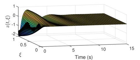
(a) State of the reaction-diffusion system $z(t,\xi)$

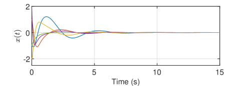
(b) State of the ODE $x(t)$

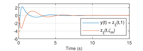
(c) Coupling channels

Figure 2: Time evolution of the coupled PDE-ODE system (15)

5 Conclusion

This paper has addressed the topic of assessing the stability of coupled systems composed of a reaction-diffusion equation and a finite-dimensional linear time-invariant ODE. The considered coupling channels are located either at the boundaries or in the domain of the PDE and consist of the input and output signals of the ODE. The reported sufficient stability conditions take the form of tractable LMIs and have been derived by adopting a spectral reduction-based method. Moreover, we have also assessed the exponential decrease to zero of the aforementioned coupling channels, particularly in the case of Neumann boundary couplings. The drawback of the present Lyapunov function based approach is that the derived stability condition are only sufficient, hence may be not satisfied by some stable reaction-diffusion systems. Nevertheless, as illustrated via the reported numerical examples, this method can be successfully applied to assess the exponential stability of coupled PDE-ODE systems for which both the open-loop PDE and ODE plants are exponentially unstable.

Appendix A End of the proof of Theorem 8

We investigate the exponential decrease of $z_{\xi}(t,\zeta_{m})$ to zero. Using the change of variable (5) and the identity $y(t)=Cx(t)$, we have $z_{\xi}(t,\zeta_{m})=w_{\xi}(t,\zeta_{m})+\mu_{m}Cx(t)$ for $t>0$. Hence, based on (17a), we only need to study the term $w_{\xi}(t,\zeta_{m})=\sum_{j\geq 1}\phi_{j}^{\prime}(\zeta_{m})w_{j}(t)$. Let $\alpha_{0}\in(3/4,1)$ and $w_{0}\in D(\mathcal{A}^{\alpha_{0}})$. Let $N_{0}\geq 1$ and $\kappa>0$ be such that $-\lambda_{n}+q_{c}\leq-\eta-\kappa$ for all $n\geq N_{0}+1$. Consider an arbitrary fixed integer $M\geq N_{0}$. Then we have

$$|w_{\xi}(t,\zeta_{m})| \leq\sum_{j\geq 1}|\phi_{j}^{\prime}(\zeta_{m})||w_{j}(t)|$$

$$\leq C_{M}\sqrt{\sum_{j=1}^{M}w_{j}(t)^{2}}+C_{\phi}\sqrt{\sum_{j\geq M+1}\lambda_{j}^{2\alpha_{0}}w_{j}(t)^{2}}$$

$$\leq C_{M}\|w(t,\cdot)\|_{L^{2}}+C_{\phi}\sqrt{\sum_{j\geq M+1}\lambda_{j}^{2\alpha_{0}}w_{j}(t)^{2}}$$

where $C_{M}=\sqrt{\sum_{j=1}^{M}\phi_{j}^{\prime}(\zeta_{m})^{2}}$ and $C_{\phi}=\sqrt{\sum_{j\geq 1}\frac{\phi_{j}^{\prime}(\zeta_{m})^{2}}{\lambda_{j}^{2\alpha_{0}}}}<\infty$. Based again on (5) and (17a) we only need to study the term $S_{M}(t)=\sum_{j\geq M+1}\lambda_{j}^{2\alpha_{0}}w_{j}(t)^{2}$. To do so, we integrate (8a) for $i\geq N_{0}+1$ and direct estimations give

$$|\lambda_{i}^{\alpha_{0}}w_{i}(t)|\leq e^{(-\lambda_{i}+q_{c})t}|\lambda_{i}^{\alpha_{0}}w_{i}(0)|$$

$$+\left(|a_{i}|\|C\|+|b_{i}|\|CA_{e}\|\right)\int_{0}^{t}\lambda_{i}^{\alpha_{0}}e^{(-\lambda_{i}+q_{c})(t-s)}\|x(s)\|\mathop{}\!\mathrm{d}s$$

$$+|b_{i}||CB|\int_{0}^{t}\lambda_{i}^{\alpha_{0}}e^{(-\lambda_{i}+q_{c})(t-s)}|w_{\xi}(s,\zeta_{m})|\mathop{}\!\mathrm{d}s$$

with $A_{e}=A+\mu_{m}BC$. For any $f\in L^{\infty}_{\mathrm{loc}}(\mathbb{R})$, we have

$$\int_{0}^{t}\lambda_{i}^{\alpha_{0}}e^{(-\lambda_{i}+q_{c})(t-s)}|f(s)|\mathop{}\!\mathrm{d}s$$

$$=e^{-\eta t}\int_{0}^{t}\lambda_{i}^{\alpha_{0}}e^{(-\lambda_{i}+q_{c}+\eta)(t-s)}\times e^{\eta s}|f(s)|\mathop{}\!\mathrm{d}s$$

$$\leq\frac{\lambda_{i}^{\alpha_{0}}}{\lambda_{i}-q_{c}-\eta}e^{-\eta t}\mathrm{ess\,sup}_{s\in[0,t]}e^{\eta s}|f(s)|$$

because $\lambda_{i}-q_{c}-\eta\geq\kappa>0$ for all $i\geq N_{0}+1$. Since $\alpha_{0}\in(3/4,1)$ we also have that $\lambda_{i}^{\alpha_{0}}/(\lambda_{i}-q_{c}-\eta)\rightarrow 0$ as $i\rightarrow+\infty$. Hence there exists a constant $\sigma=\sigma(\alpha_{0})>0$, independent of $M$, so that $\lambda_{i}^{\alpha_{0}}/(\lambda_{i}-q_{c}-\eta)\leq\sigma$ for all $i\geq N_{0}+1$. Combining the latter estimates, we infer that

$$|\lambda_{i}^{\alpha_{0}}w_{i}(t)|\leq e^{-\eta t}|\lambda_{i}^{\alpha_{0}}w_{i}(0)|$$

$$+\sigma\left(|a_{i}|\|C\|+|b_{i}|\|CA_{e}\|\right)e^{-\eta t}\sup_{s\in[0,t]}e^{\eta s}\|x(s)\|$$

$$+\sigma C_{M}|b_{i}||CB|e^{-\eta t}\sup_{s\in[0,t]}e^{\eta s}\|w(s,\cdot)\|_{L^{2}}$$

$$+\sigma C_{\phi}|b_{i}||CB|e^{-\eta t}\sup_{s\in[0,t]}e^{\eta s}\sqrt{S_{M}(s)}$$

for all $i\geq N_{0}+1$ and all $t\geq 0$. The use of Young’s inequality and summing for $i\geq M+1\geq N_{0}+1$ we obtain that

$$S_{M}(t)\leq 5e^{-2\eta t}S_{M}(0)$$

$$+5\sigma^{2}\left(\|\mathcal{P}_{M}a\|_{L^{2}}^{2}\|C\|^{2}+\|\mathcal{P}_{M}b\|_{L^{2}}^{2}\|CA_{e}\|^{2}\right)$$

$$\phantom{+}\;\times e^{-2\eta t}\sup_{s\in[0,t]}e^{2\eta s}\|x(s)\|^{2}$$

$$+5\sigma^{2}C_{M}^{2}\|\mathcal{P}_{M}b\|_{L^{2}}^{2}|CB|^{2}e^{-2\eta t}\sup_{s\in[0,t]}e^{2\eta s}\|w(s,\cdot)\|_{L^{2}}^{2}$$

$$+5\sigma^{2}C_{\phi}^{2}\|\mathcal{P}_{M}b\|_{L^{2}}^{2}|CB|^{2}e^{-2\eta t}\sup_{s\in[0,t]}e^{2\eta s}S_{M}(s)$$

for all $t\geq 0$, hence

$$\sup_{s\in[0,t]}e^{2\eta s}S_{M}(s)\leq 5S_{M}(0)$$

$$+5\sigma^{2}\left(\|\mathcal{P}_{M}a\|_{L^{2}}^{2}\|C\|^{2}+\|\mathcal{P}_{M}b\|_{L^{2}}^{2}\|CA_{e}\|^{2}\right)$$

$$\phantom{+}\;\times\sup_{s\in[0,t]}e^{2\eta s}\|x(s)\|^{2}$$

$$+5\sigma^{2}C_{M}^{2}\|\mathcal{P}_{M}b\|_{L^{2}}^{2}|CB|^{2}\sup_{s\in[0,t]}e^{2\eta s}\|w(s,\cdot)\|_{L^{2}}^{2}$$

$$+5\sigma^{2}C_{\phi}^{2}\|\mathcal{P}_{M}b\|_{L^{2}}^{2}|CB|^{2}\sup_{s\in[0,t]}e^{2\eta s}S_{M}(s).$$

Since $\|\mathcal{P}_{M}b\|_{L^{2}}\rightarrow 0$ when $M\rightarrow+\infty$, we infer the existence of a large enough integer $M\geq N_{0}+1$, independent of the initial condition $w_{0}\in D(\mathcal{A}^{\alpha_{0}})$, such that $5\sigma^{2}C_{\phi}^{2}\|\mathcal{P}_{M}b\|_{L^{2}}^{2}|CB|^{2}<1$. Fixing such a $M\geq N_{0}+1$ and because all the supremums appearing in the latter estimate are finite (recall that $\mathcal{A}^{\alpha_{0}}w\in\mathcal{C}^{0}([0,\infty);L^{2}(0,1))$), we obtain the existence of a constant $M_{4}>0$ such that

$$\sup_{s\in[0,t]}e^{2\eta s}S_{M}(s) \leq M_{4}S_{M}(0)+M_{4}\sup_{s\in[0,t]}e^{2\eta s}\|x(s)\|^{2}$$

$$\phantom{\leq}\;+M_{4}\sup_{s\in[0,t]}e^{2\eta s}\|w(s,\cdot)\|_{L^{2}}^{2}$$

for all $t\geq 0$. Noting that $S_{M}(0)\leq\|\mathcal{A}^{\alpha_{0}}w_{0}\|_{L^{2}}^{2}$, the claimed conclusion follows from (5) and (17a). In the case $w_{0}\in D(\mathcal{A})$, it can easily be seen that $D(\mathcal{A})\subset D(\mathcal{A}^{\alpha_{0}})$ and $\|\mathcal{A}^{\alpha_{0}}w_{0}\|_{L^{2}}^{2}\leq\|w_{0}\|_{L^{2}}^{2}+\|\mathcal{A}w_{0}\|_{L^{2}}^{2}$, which gives (17b) and concludes the proof.

References

• [1] Mohamadreza Ahmadi, Giorgio Valmorbida, and Antonis Papachristodoulou. Dissipation inequalities for the analysis of a class of PDEs. Automatica, 66:163–171, 2016.
• [2] Habib Ayadi. Exponential stabilization of cascade ODE-linearized KdV system by boundary dirichlet actuation. European Journal of Control, 43:33–38, 2018.
• [3] Matthieu Barreau, Frédéric Gouaisbaut, Alexandre Seuret, and Rifat Sipahi. Input/output stability of a damped string equation coupled with ordinary differential system. International Journal of Robust and Nonlinear Control, 28(18):6053–6069, 2018.
• [4] Matthieu Barreau, Carsten Scherer, Frédéric Gouaisbaut, and Alexandre Seuret. Integral quadratic constraints on linear infinite-dimensional systems for robust stability analysis. In IFAC World Congress, 2020.
• [5] Matthieu Barreau, Alexandre Seuret, and Frédéric Gouaisbaut. Exponential Lyapunov stability analysis of a drilling mechanism. In 2018 IEEE Conference on Decision and Control (CDC), pages 6579–6584. IEEE, 2018.
• [6] Matthieu Barreau, Alexandre Seuret, Frédéric Gouaisbaut, and Lucie Baudouin. Lyapunov stability analysis of a string equation coupled with an ordinary differential system. IEEE Transactions on Automatic Control, 63(11):3850–3857, 2018.
• [7] Lucie Baudouin, Alexandre Seuret, and Frédéric Gouaisbaut. Stability analysis of a system coupled to a heat equation. Automatica, 99:195–202, 2019.
• [8] Nikolaos Bekiaris-Liberis and Miroslav Krstic. Compensating the distributed effect of a wave pde in the actuation or sensing path of MIMO LTI systems. Systems & Control Letters, 59(11):713–719, 2010.
• [9] Abed Boulouz, Hamid Bounit, and Said Hadd. Well-posedness and exponential stability of boundary control systems with dynamic boundary conditions. Systems & Control Letters, 147:104825, 2021.
• [10] Jean-Michel Coron and Emmanuel Trélat. Global steady-state controllability of one-dimensional semilinear heat equations. SIAM Journal on Control and Optimization, 43(2):549–569, 2004.
• [11] Jean-Michel Coron and Emmanuel Trélat. Global steady-state stabilization and controllability of 1D semilinear wave equations. Commun. Contemp. Math., 8(04):535–567, 2006.
• [12] Jamal Daafouz, Marius Tucsnak, and Julie Valein. Nonlinear control of a coupled PDE/ODE system modeling a switched power converter with a transmission line. Systems & Control Letters, 70:92–99, 2014.
• [13] Amritam Das, Sachin Shivakumar, Matthew Peet, and Siep Weiland. Robust analysis of uncertain ODE-PDE systems using PI multipliers, PIEs and LPIs. In 2020 59th IEEE Conference on Decision and Control (CDC), pages 634–639. IEEE, 2020.
• [14] Aditya Gahlawat and Matthew M Peet. A convex sum-of-squares approach to analysis, state feedback and output feedback control of parabolic PDEs. IEEE Transactions on Automatic Control, 62(4):1636–1651, 2016.
• [15] Wei He and Shuzhi Sam Ge. Cooperative control of a nonuniform gantry crane with constrained tension. Automatica, 66:146–154, 2016.
• [16] Miroslav Krstic. Compensating a string PDE in the actuation or sensing path of an unstable ODE. IEEE Transactions on Automatic Control, 54(6):1362–1368, 2009.
• [17] Miroslav Krstic. Compensating actuator and sensor dynamics governed by diffusion PDEs. Systems & Control Letters, 58(5):372–377, 2009.
• [18] Miroslav Krstic and Nikolaos Bekiaris-Liberis. Compensation of infinite-dimensional input dynamics. Annual Reviews in Control, 34(2):233–244, 2010.
• [19] Hugo Lhachemi and Christophe Prieur. Feedback stabilization of a class of diagonal infinite-dimensional systems with delay boundary control. IEEE Transactions on Automatic Control, 66(1):105–120, 2020.
• [20] Hugo Lhachemi, David Saussié, and Guchuan Zhu. Boundary feedback stabilization of a flexible wing model under unsteady aerodynamic loads. Automatica, 97:73–81, 2018.
• [21] Jian Li and Yungang Liu. Adaptive stabilization of coupled PDE–ODE systems with multiple uncertainties. ESAIM: Control, Optimisation and Calculus of Variations, 20(2):488–516, 2014.
• [22] Vivek Natarajan. Compensating PDE actuator and sensor dynamics using Sylvester equation. Automatica, 123:109362, 2021.
• [23] Serge Nicaise, Julie Valein, and Emilia Fridman. Stability of the heat and of the wave equations with boundary time-varying delays. Discrete and Continuous Dynamical Systems¿ Series S, 2(3):559, 2009.
• [24] Yury Orlov. On general properties of eigenvalues and eigenfunctions of a Sturm–Liouville operator: comments on ”ISS with respect to boundary disturbances for 1-D parabolic PDEs”. IEEE Transactions on Automatic Control, 62(11):5970–5973, 2017.
• [25] Amnon Pazy. Semigroups of linear operators and applications to partial differential equations, volume 44. Springer Science & Business Media, 2012.
• [26] Matthew M Peet. A Partial Integral Equation (PIE) representation of coupled linear PDEs and scalable stability analysis using LMIs. Automatica, 125:109473, 2021.
• [27] Matthew M Peet. Representation of networks and systems with delay: DDEs, DDFs, ODE–PDEs and PIEs. Automatica, 127:109508, 2021.
• [28] Ricardo Sanz, Pedro García, and Miroslav Krstic. Robust compensation of delay and diffusive actuator dynamics without distributed feedback. IEEE Transactions on Automatic Control, 64(9):3663–3675, 2018.
• [29] Sachin Shivakumar, Amritam Das, Siep Weiland, and Matthew M Peet. A generalized LMI formulation for input-output analysis of linear systems of ODEs coupled with PDEs. In 2019 IEEE 58th Conference on Decision and Control (CDC), pages 280–285. IEEE, 2019.
• [30] Gian Antonio Susto and Miroslav Krstic. Control of PDE–ODE cascades with neumann interconnections. Journal of the Franklin Institute, 347(1):284–314, 2010.
• [31] Shuxia Tang and Chengkang Xie. State and output feedback boundary control for a coupled PDE–ODE system. Systems & Control Letters, 60(8):540–545, 2011.
• [32] Ji Wang and Miroslav Krstic. Output feedback boundary control of a heat PDE sandwiched between two ODEs. IEEE Transactions on Automatic Control, 64(11):4653–4660, 2019.
• [33] Jun-Min Wang, Jun-Jun Liu, Beibei Ren, and Jinhao Chen. Sliding mode control to stabilization of cascaded heat PDE–ODE systems subject to boundary control matched disturbance. Automatica, 52:23–34, 2015.
• [34] Huai-Ning Wu and Jun-Wei Wang. Static output feedback control via PDE boundary and ODE measurements in linear cascaded ODE–beam systems. Automatica, 50(11):2787–2798, 2014.