Quasi-structured quadrilateral meshing in Gmsh –
a robust pipeline for complex CAD models

Abstract

We propose an end-to-end pipeline to robustly generate high-quality quadrilateral meshes for complex CAD models. An initial quad-dominant mesh is generated with frontal point insertion guided by a locally integrable cross field and a scalar size map adapted to the small CAD features. After triangle combination and midpoint-subdivision into an all-quadrilateral mesh, the topology of the mesh is modified to reduce the number of irregular vertices. The idea is to preserve the irregular vertices matching cross-field singularities and to eliminate the others. The topological modifications are either local and based on disk quadrangulations, or more global with the remeshing of patches of quads according to predefined patterns. Validity of the quad mesh is guaranteed by monitoring element quality during all operations and reverting the changes when necessary. Advantages of our approach include robustness, strict respect of the CAD features and support for user-prescribed size constraints. The quad mesher, which is available in Gmsh, is validated and illustrated on two datasets of CAD models.

1 Introduction

There are essentially two main scientific communities that have been historically interested in generating quadrilateral meshes: the engineering analysis community, as these meshes are good geometrical support for the finite element and finite volume methods, and the computer graphics community which, besides application in numerical simulations, has good use for them in surface modeling (e.g. subdivision surface) and texturing.

The engineering analysis community has been working on algorithms for generating quadrilateral meshes for several decades, leading to two main categories of industrial-grade techniques. The first one is to manually decompose the CAD model in quadrilateral patches, with potentially some semi-automatic assistance. The patches are then filled with quads while considering user element sizing specifications,e.g. anisotropic quads with geometric progression from the boundary layers. This approach is very time-consuming and is mainly used for demanding numerical simulations such as CFD. On the other end, various fully automatic approaches have been developed for generating unstructured quadrilateral meshes, such as paving [5] or Blossom-Quad [37] with frontal Delaunay point insertion [38]. Their disadvantages are the potentially high number of irregular vertices, the non-regular alignment of edges in the mesh (affecting smoothness of gradients in simulations) and the lack of user control. Both approaches are now available in most mesh generation packages, including Gmsh [18].

In the last decade, the computer graphics research community has thoroughly developed and explored cross-field based techniques for quadrilateral meshing, with a focus on the automatic generation of high-quality block-structured quadrilateral meshes, or equivalently coarse quadrilateral layouts which partition the object surfaces into conforming quadrilateral patches. Finite element practitioners quickly became interested in these ideas because of their potential to replace semi-automatic block-structured mesh generators by fully automatic ones. A fruitful line of research revolves around the construction of a global parametrization from which we can extract an all-quadrilateral mesh. The global parametrization is a discontinuous mapping that maps a 2D grid from the parameter domain to the model surface, with discontinuities to allow for the existence of irregular vertices (Sec. 1.2 for more details). The work presented in the current paper started from an attempt to apply such a global parametrization technique in the context of CAD meshing in Gmsh, as explained later (Sec. 2).

The quasi-structured quadrilateral meshing pipeline that we propose exploits the strength of both worlds. We rely on the robustness of automatic unstructured quad meshing techniques, and we use the topological and geometrical information from cross fields to transform unstructured meshes into high-quality ones, with few but well located irregular vertices. Our approach has many advantages which are important for CAD meshing: it always produces valid quadrilateral meshes, it strictly respects all CAD features and it supports non-uniform element size maps. The new quad mesher is integrated in Gmsh (version 5 and higher) [18] and its implementation is open-source.

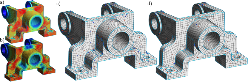
Figure 1: The quasi-structured quad meshing pipeline applied on the model M3 [24] (111 CAD corners, 169 curves, 60 faces). The cross field and its associated conformal scaling is computed on an initial triangulation (a). The size map (b) combines the cross field scaling and is adapted to the small CAD features. The initial unstructured all-quadrilateral mesh (c) is computed with a frontal approach, and contains $3429/54982$ irregular vertices. After cavity remeshing, the final quasi-structured mesh (d) contains $606/56743$ irregular vertices. $78$ of them match the cross field singularities (a) and the others allow the mesh size transitions (b).

1.1 Overview

This paper proposes a robust end-to-end pipeline to build quasi-structured quadrilateral meshes for arbitrary CAD models. Our only requirement of the input CAD model is that it is valid in the sense that it is possible to generate a triangulated mesh with standard techniques. This includes non-manifold surfaces, which typically appear when the CAD models contains multiple volumes. By quasi-structured quadrilateral mesh, we mean that the number of irregular vertices is small compared to the usual unstructured techniques, and close or equal to the number of irregular vertices obtained with cross-field based parametrization approaches when the target mesh size is smaller than the CAD features (e.g. Fig. 2). Our meshing pipeline, illustrated on Fig. 1, is:

1. Compute a scaled cross field on each CAD face, using an initial triangulation. The cross directions are computed with a fast multilevel heat diffusion approach and a conformal scaling is obtained by solving a linear system, see Sec. 3.

2. Compute a global metric field (combined direction field and scalar size map) from the prescribed sizing constraints, the small CAD features and the conformal scaling associated to the cross field, see Sec. 4.

3. Generate the meshes of the CAD curves considering the size map and global topological constraints, see Sec. 4.3.

4. Generate the quasi-structured quadrilateral meshes of the simple CAD faces which match predefined patterns, see Sec. 6.1.2.

5. Generate unstructured quadrilateral meshes on the remaining CAD faces, using a frontal approach guided by the cross field scaled by the size map, see Sec. 5.

6. Modify the quadrilateral mesh topology to make it quasi-structured, by removing defects with local disk-quadrangulation operations (Sec. 6.3) and by remeshing convex cavities to match the cross field singularities (Sec. 6.2).

With this pipeline the ultimate focus is on robustness, which has precedence over all other considerations. The unstructured quad mesh is geometrically and topologically valid by construction (quad-dominant mesh subdivided into full-quad). For all the remeshing operations, we always verify that the topology and the geometry remain valid, and we reject the ones which invalidate or degrade the element qualities.

The scaled cross field guides the unstructured point insertion and its singularities are used to constrain the cavity remeshing. All the steps produce valid outputs even if the cross field is not accurate or is topologically invalid. The key idea to robustly deal with complex CAD models is to use the cross field as an auxiliary tool without entirely relying upon it, since it may and usually contains many defects (does not take small CAD features or quantization into account, may have wrong singularities, may have insufficient accuracy).

Figure 2.2. illustrates our pipeline for a single surface. In practice, this surface should be seen as a particular CAD face of a larger model, so its 1D boundary mesh cannot be modified without affecting its neighbors. This compatibility constraint between the meshes of adjacent CAD faces is one of the major sources of difficulty when dealing with complex CAD models. We can look at a more realistic CAD model on Fig. 1, where the CAD faces are meshed independently. After topological improvement (Fig. 1.d.), there are still irregular vertices that do not match singularities from the cross field. These are due to the curve quantization which follows the size map (Fig. 1.b.), and which is necessary to take small CAD features into account. For more detailed discussions and applications to complex models, see Sec. 7.

Because we present an end-to-end mesher, a lot of ground is covered and it is not practical to describe everything in details. We try to provide extensive references to the literature so the reader can refer to them for further details on specific parts of the pipeline.

1.2 Related work

Unstructured quadrilateral meshing

A classic approach to generate unstructured quadrilateral meshes is to start from the boundary and to progressively insert points in the surface. The paving algorithm [5] directly generates quadrilateral in an advancing-front fashion. Indirect methods first generate a triangulation with well-placed vertices then merge pairs of triangles into quads [25, 9]. There are many ways on how to choose the merged triangles. In Q-Morph [30], triangles are transformed in quadrilaterals with an advancing-front algorithm. BlossomQuad [37] computes a global perfect matching to optimally pair triangles, which works especially well with right-angled triangles generated by [38].

These methods generally suffer from degraded mesh quality and high vertex irregularity, especially at front collisions. But on the other hand, they are highly robust. Even when a pure quad mesh cannot be obtained directly, it’s always possible to perform a midpoint subdivision, also called Catmull-Clark subdivision, to obtain an all-quadrilateral mesh by splitting the triangles into three quads and the initial quads into four sub-quads.

Cross fields

In the last decade, cross fields [19, 34, 31] have become very popular for quadrilateral meshing. Crosses can be seen as infinitesimal quads and they have topological structures which match quad mesh topology, such as cross singularities which have one-to-one correspondence with quad mesh irregular vertices [12, 35].

Cross field can be computed by minimizing a smoothness energy, either by directly optimizing the angles [6] or by smoothing a vector representation with a way to ensure that the variables stay crosses, such as Ginzburg-Landau penalization [3] or with iterative projection [46]. In this paper, we use the MBO method [46] where we alternate diffusion and projection, with varying time stepping [32] and additional optimizations (Sec. 3.1).

It is important to note that cross fields are not integrable by default. On a cut domain, a cross field can be seen as two orthogonal unit vector fields. To have integrable vector fields, it is necessary to break the orthogonality [39] or to scale the amplitudes. Ray N. et al. [34] introduce a correction step to make the two vector fields curl-free. Another approach it to solve a linear problem to compute a global conformal scaling from the cross field singularities [12, 4], which can be applied to both vector fields. We compute a similar conformal scaling (Sec. 3.3) by canceling a Lie bracket, without using the cross field singularities.

There are various ways to exploit the cross field information for quad meshing. It can be used as a directional guide for frontal point insertion, as in [38] and in our unstructured initialization (Sec. 5). A popular alternative is to directly build the quadrilateral layout by tracing separatices in the vector fields, e.g. [13, 29, 33]. Another common approach is to integrate the cross-field by computing a parametrization.

Cross field based parametrization

A parametrization associated to a cross field is usually made of two scalar fields $u,v$ such that their gradients are aligned with the cross field directions. Such parametrization is a mapping from the 2D parameter space to the 3D surface. The mapping discontinuities, which are cuts on the model surface, allow for the existence of irregular vertices on the quadrilateral mesh. QuadCover [21] introduced globally coherent parametrization to integrate a cross field, with integer grid-preserving constraints on a cut-graph to ensure global coherency. This idea have been highly refined and improved in the form of integer grid mapping [6, 8, 14, 17]. With these approaches, the irregular vertices in the final quad mesh strictly match the cross field singularities. Alternatively, the parametrization formulation can be relaxed, either by computing local parametrizations [20] or a loosely constrained global parametrization which relies on periodic functions [34]. In both cases, there are additional irregular vertices in the final quad mesh introduced by the relaxation. Our experience with a global parametrization attempt is detailed in Sec. 2.

Topological meshing and modifications

Unstructured quadrilateral meshing methods do not naturally offer the regularity and structure obtained with global parametrization methods. Is it possible however to reduce the number of irregular nodes and improve quality by performing topological modifications on an unstructured quad mesh. Due to topological constraints in quadrilateral meshes (Sec. 1.3), there is no simple local operation such as the edge-split or edge-collapse, but there are still many possibilities, some global such as chord collapsing [15] and other more local [16] but which are restricted to specific vertex-valence configurations.

In this work, we are particularly interested in operations that modify the content of a patch of quads inside the mesh, called cavity, without changing its boundary. For triangular and pentagonal cavities, Bunin G. [11] has shown that we can find a topological quad mesh replacement with a single irregular vertex by solving a linear system. This local clean-up is a fundamental piece of the Jaal quad mesher [45], with a later extension to more generic replacement patterns [44].

This problem of remeshing a cavity is equivalent to the problem of topologically finding a quadrilateral mesh for a given polyline boundary. It has been studied in the computer graphics context [49], with a generic integer linear formulation for generic $N$-sided patches [41]. The local remeshing operator has been used in interactive software to help users improve their quad meshes [26].

1.3 Topology of quadrilateral meshes

In a polygonal mesh, the Euler-Poincaré formula $\chi=n-n_{e}+n_{f}$ provides a relationship between the $n$ vertices, the $n_{e}$ edges, the $n_{f}$ facets and the Euler-Poincaré characteristic $\chi$ of the associated surface, which is given by the relation $\chi=2-2g-b$ with $b$ the number of holes and $g$ the number of handles.

In a quadrilateral mesh, we can follow [3] to derive the relationship

$$4n_{f}=\sum_{k}4(n-n_{b}-n_{k})+2(n_{b}-m_{k})+(4-k)n_{k}+(2-k)m_{k}$$

between the number of vertices of various indices. $m_{k}$ is the number of boundary vertices with valence $2-k$ and $n_{k}$ the number of interior vertices with valence $4-k$. When $k\neq 0$, the vertices are said to be irregular of index $k$. By combining this relation with the Euler formula, we obtain [3] the relation (1) between the number of irregular vertices on the boundary and on the interior in a quadrilateral mesh:

$$\chi=\sum_{k}{k\over 4}(n_{k}+m_{k})$$ (1)

This formula has some interesting topological implications: regular vertices do not count, pairs of irregular vertices of opposite indices cancel themselves (e.g. valence three ($k=1$) and valence five ($k=-1$)), surfaces with $\chi=0$ (topological ring) are the only ones that admit fully regular quadrilateral meshes (only valence four inside and valence two on the boundary).

We will see later in this paper that it is possible to generate quadrilateral meshes with interior irregular vertices of indices $+1$ and $-1$ only, corresponding respectively to quadrilateral valences of $3$ and $5$. This restriction to irregular vertices of low index is usually better to generate high-quality quads, as irregular vertices are associated with geometric distortions. In this paper, we thus restrict ourselves to irregular boundary vertices of valence $1,3$ and $4$, i.e. of indices $1,-1$ and $-2$, and to interior irregular vertices of valences $3$ and $5$, i.e. of indices $+1,-1$. The relation (1) between the surface Euler-Poincaré characteristic and the quadrilateral mesh irregular vertices becomes:

$$n_{1}-n_{-1}=4\chi+m_{-1}-m_{1}+2m_{-2}$$ (2)

We say that a quadrangulation of a surface with Poincaré characteristic $\chi$ is minimally irregular if its contains exactly $4|\chi|$ isolated irregular vertices of index $\mbox{sign}(\chi)$ (counting the boundary irregular vertices). For example, in the surface of Fig. 2, we have $\chi=-6$ and $m_{1}=4$ convex corners, so we should have $n_{-1}=28$ irregular vertices of valence five to be minimally-irregular.

A dipole is a pair of irregular vertices with opposite indices $+1$ and $-1$. Adding dipoles to a minimally irregular quad mesh may be necessary, for example to allow mesh size variations. A mesh is called quasi-structured if it contains $4|\chi|$ isolated irregular vertices of index $\mbox{sign}(\chi)$ plus a small amount of dipoles. We use the loosely defined adjective small because it is a priori impossible to determine the minimum amount of dipoles that are necessary for a given application.

2 Context and motivation

The more general context around this article is our effort to build a robust high-quality quadrilateral mesher in Gmsh that actually works. What we mean is that a user should be able to produce a high quality quad mesh on any valid CAD model by only loosely specifying the target element sizes, as it is the case for triangular meshing.

Global parametrization

Our initial attempt, inspired by state-of-the-art global parametrization techniques [6, 14], was to build a seamless uv-parametrization from a cross field and then extract a quad-layout. Figure 2.1. illustrates the different steps for the construction of a quadrilateral mesh with this approach. Parametrization based techniques cut and flatten the surface of the domain. The cuts (in green on Figure Fig. 2.1.b.) allow to find a continuous branch of the cross field and to build a seamless $uv$ parametrization (see Fig. 2.1.b.) by solving a linear system with an alignment energy (gradients of $u$ and $v$ must be parallel to the cross field) and specific grid-compatibility linear constraints on the cut graph. To avoid the technical difficulties associated with the integer variables in the standard mixed-integer formulation [21, 6], we directly extracted the (conformal) quadrilateral layout from the iso-value separatrices in the $uv$ parametrization (Fig. 2.1.c.). We replaced the integer variables and associated global quantization [14] by explicit topological simplification (chord collapse) of the quad layout, since we initially had lot of very thin quad patches as we were doing no snapping or geometric thresholding. The resulting quadrilateral mesh (Fig. 2.1.d.) was of very high quality, when it worked.

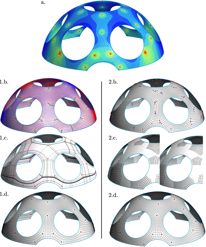
Figure 2: Two approaches to build a quasi-structured mesh of a surface. In the global parametrization approach, we build a seamless parametrization (1.b.) by integrating a scaled cross field (a.), then we extract a conformal quadrilateral layout (1.c.) and build the final quad mesh (1.d.) by simplyfing the subdivided layout. In the second approach (this paper), we first build a unstructured quadrilateral mesh (2.b.) with a frontal approach guided by the scaled cross field (a.), then we apply cavity remeshing (2.c.) to eliminate unnecessary irregular vertices while preserving the cross field singularities. The final quad mesh (2.d) is very similar to the one obtained with the global parametrization approach and has the same number of irregular vertices.

Even though we were quite excited with our initial results, we failed to generalize the approach into a robust mesher able to handle large and complex CAD models. It took us considerable amount of time and energy to obtain an implementation that is still in a very beta version state. The amount of non-reusable code that is required for generating the quad mesh of Fig. 2.1.d. is quite large and only works when the cross field topology is in perfect accordance with the topology of the surface to mesh, which is often not the case when smoothing continuous representations of crosses. On a given CAD face, the difficultly mainly comes from the linear system that computes the $uv$-parametrization: it must be strictly right. If there is a small incoherence in the grid-compatibility constraints, e.g. due to wrong flagging of singularities, there will be no solution, or a useless one. Even more difficult is the generalization to large CAD models with hundreds of CAD faces, potentially non-manifold at CAD curves if there are multiple volumes. To avoid separatrices winding up around the models for thousands of turns before coming back to their origin, we build independently the quad layouts on each CAD face and then try to reunite them. The union of the quad layouts has many T-junctions on the CAD curves. One potential idea is to use a global integer quantization [14] to assign compatible non-zero integers to each edge of the global quad layout (with T-junctions). However, we soon discovered that often there is no non-degenerate solution: the constraints can be circular, e.g. $a+b=c,c=d,d=e,e=a$ leading to $b=0$.

While some issues could be fixed, we do not foresee a robust implementation of that algorithm that would work for industrial grade models within a reasonable timescale. Moreover, such long codes are prone to bugs and are difficult to maintain. Of course, the mesh shown on Fig. 2.1.d. is exactly the what most finite element practitioners are willing to use. The main question became:

Can we obtain such high quality mesh using an approach that is both simple and robust?

Unstructured quad meshing

Our experience in indirect quad meshing [37, 38] has been positive in term of industrial use. Indirect quad meshers are essentially based on existing surface meshers (very small amount of extra coding). The transformation of a triangular mesh into a quad mesh by combination of pairs of triangles is an extra step that is simple, robust and efficient [37, 9]. Indirect quad meshers are thus able to treat models of arbitrary complexities with a run time that is not larger than standard triangular meshing. The main drawback of quad meshes generated in an indirect fashion is that they cannot be considered as block-structured or quasi-structured because they contain an arbitrary large number of irregular vertices.

All those reasons have convinced us to move to a new approach that would take the best of both worlds. We have decided to use our existing indirect meshing technology and build an initial unstructured quad mesh (Fig. 2.2.b.) that is mostly aligned with a cross field. Then, information provided by the cross field is used to modify this unstructured mesh and make it quasi-structured, i.e. with only a few irregular vertices.

Besides working even if the cross field is inaccurate, there is another big advantage: we can use a external non-uniform size maps to locally control the mesh size, independently of the cross field. In practice, we compute a size map adapted the small CAD features, which has proven to be invaluable when dealing with complex models.

Gmsh surface-to-volume philosophy

Gmsh’s usual meshing pipeline is essentially ”surface to volume”, also called ”bottom-up”. Model curves are discretized (meshed) at first. Then, model surfaces are triangulated/quadrangulated based on a boundary discretization that is imposed by the model curves. Finally, model volumes are tessellated. This approach has many advantages: strict respect of CAD features, flexibility (different meshers can be used for different CAD entities), robustness (we can replace with a different approach on a entity if one failed), easy parallelism, and the automatic support for non-manifold surfaces in models with multiple volumes. Sometimes there is no solution for the meshing of an entity given its boundary mesh (e.g. too coarse). In these cases, the boundary mesh is modified (usually a split of some elements) and the meshing of the entities that share this boundary is restarted, until a solution is found or the maximal number of tries is exhausted.

We also follow this philosophy with our quad mesher to benefit from the same advantages, but it should be noted that it has a significant drawback when meshing a CAD face: the boundary mesh (from the boundary CAD curves) is locked and cannot be changed. Thus, the curve quantization (Sec. 4.3) is very important. The size map, which controls the curve sampling, must be global and smooth on the CAD curves to have coherent meshes on the adjacent CAD faces. With our current approach, there are some irregular vertices in the final mesh that are due to non-optimal curve quantization, and which could be eliminated with further work (Sec. 8).

3 Scaled cross field computation

In our pipeline, cross fields fulfill two roles: (a) they guide the frontal point insertion in the unstructured quadrilateral mesher (Sec. 5) and (b) they have singularities (Sec. 3.2) which correspond to irregular vertices that we want to keep during the topological modifications that lead to the final quasi-structured mesh (Sec. 6.2). The cross field is computed with a fast multilevel diffusion algorithm (Sec. 3.1) which alternates diffusion steps and projection on the cross space. Then, to improve the accuracy of the following point insertion, we scale the cross field to make it integrable by computing its conformal scaling (Sec. 3.3), which can be seen as a size map (up to a constant) useful to accommodate rotations in the cross field.

3.1 Fast cross field computation with multilevel diffusion

A cross field is a field defined on a surface with values in the quotient space $S^{1}/Q$, where $S^{1}$ is the circle group and $Q$ is the group of quadrilateral symmetry. It associates to each point of the surface to be meshed a cross made of four unit vectors orthogonal with each other in the tangent plane of the surface. In our case, we compute one cross field per CAD face, with crosses aligned with the CAD curves bounding the face.

Cross representation

To represent the crosses, we use the standard unit vector representation $\mathbf{u}=(\cos(4\theta),\sin(4\theta))=(u_{1},u_{2})$ [19] where $\theta$ is the angle of one of the four branches with a local reference frame. Contrary to the naive angle representation $\theta$, the vector representation $\mathbf{u}$ is invariant to the quadrilateral symmetries and suitable for linear finite element interpolation. As the linear combination of unit vectors is usually not a unit vector, the interpolated values inside triangles are not a strictly representations of crosses, but the crosses can be recovered easily by projecting on the unit circle, i.e. normalizing the vector representation.

Finite element discretization

To discretize the vector field representation of the cross field, we define one cross at each edge of the triangulation and use the Crouzeix-Raviart interpolation, as in [3]. The unknowns of the cross field problem are the representation vector field components $u_{1},u_{2}$ at each edge $e_{ij}$. As we want the cross field to be aligned the surface boundaries, the Dirichlet boundary conditions are $\mathbf{u}=(\cos(0),\sin(0))=(1,0)$ at each boundary edge.

Smoothing with the heat equation

To have a smooth cross field inside the domain, the natural approach is to minimize the Dirichlet energy:

$$\min_{|\mathbf{u}(\mathbf{x})|=1}\int_{\Omega}\|\nabla\mathbf{u}\|^{2}$$

This objective function is non-linear as the crosses live in the quotient space $S^{1}/Q$, which is equivalent to the cross representation being on the unit circle, i.e. $\forall\mathbf{x}\in\Omega,|\mathbf{u}(\mathbf{x})|=1$. A standard relaxation is to allow the cross representation to leave the unit circle, but they should stay close to it. Minimizing the Dirichlet energy by directly solving the Laplacian of the vector representation, i.e. $\nabla^{2}\mathbf{u}={\bf 0}$, is not appropriate as the values may collapse to ${\bf 0}$ far from the boundary. One elegant solution to this problem is to solve a Ginzburg-Landau non-linear equation to penalize the values leaving the cross manifold [3], but this approach is too expensive for large problems. A more efficient alternative is the MBO approach [46], where one alternates heat diffusion (Eq. 3) and projection (Eq. 4) steps. A further refinement [32] developed for 3D cross fields is to start with large diffusion time-steps and progressively decrease them. In this work, we also use decreasing diffusion time-steps but we select them according to the mesh size considerations, and we regroup them in levels to allow for re-use of the matrix factorization computed by a direct linear solver.

Diffusion: $${\partial\mathbf{u}\over\partial t}=\alpha\nabla^{2}\mathbf{u}$$ (3)

Projection: $$\mathbf{u}\leftarrow\frac{\mathbf{u}}{\|\mathbf{u}\|}$$ (4)

Multilevel strategy

When dealing with large CAD models, there are usually geometric features at many scales. Using a uniform mesh that is sufficiently fine to capture the smallest features is expensive and wasteful, as the cross field is mainly smooth far from the boundaries. In practice, we use triangulated meshes adapted to the geometric features, which can lead to edge lengths varying by many order of magnitudes in the mesh.

Our strategy is to iteratively resolve the cross field at various scales, which we call levels. Each level is characterized by a different diffusion coefficient, the $\alpha$ in (Eq. 3). Intuitively, we start with large diffusion lengths and progressively decrease to eventually capture the smallest cross field features. Beside being suited for non-uniform meshes, it is also a great way to accelerate computations on uniform triangulations. This approach is very fast: the cost of computing an accurate cross field is similar to the cost of solving a few linear systems, as we are re-using matrix factorizations inside levels.

After generating a triangulated mesh of the whole CAD model, with mesh sizes adapted to the CAD features, we compute the cross-field on each surface independently. As the boundary condition (cross tangency) is the same on both sides of a curve separating two CAD surfaces, the solutions will be compatible and we can regroup them at the end.

For a given triangulation $T$ of a surface $\mathcal{S}$, we pre-compute $N$ diffusion coefficients that will be used for the $N$ successive heat diffusion levels. At each level, we successively solve the heat equation and project the solution, until the cross field no longer changes. In a way, we are solving the cross field problem (minimizing the Dirichlet energy) for a given resolution. Typically, the appropriate number of levels is between $5$ and $10$ for a large model but a lower value around $3$ or $4$ is sufficient for a CAD face. We chose the initial (largest) and final (smallest) coefficients as

$$\alpha_{\text{initial}}=(0.1*d)^{2}\text{ and }\alpha_{\text{final}}=(3*h_{\text{min}})^{2}$$

with $d$ the length of the surface bounding box diagonal and $h_{\text{min}}$ the smallest edge length. The large initial time-step allows a first coarse diffusion of the boundary conditions and the final small time-step allows a local smoothing of the crosses at the finer mesh sizes. Between these extremities, we use linearly interpolated time-steps. While these choices are quite arbitrary, they are the results of many experimentations and we have found that they work pretty well on a large variety of CAD models with features at many scales.

The speed of our approach comes from the re-use of linear factorizations inside each level. From the heat diffusion equation (Eq. 3), we derive the discrete version, using finite element for spatial and backward Euler for time discretization:

$$M(U_{i+1}-U_{i})=-\alpha KU_{i}$$

with $M$ the mass and $K$ the stiffness Crouzeix-Raviart matrices. For more details about the stiffness matrix assembly, one can refer to [3] as our coefficients are the same. With Crouzeix-Raviart, the mass matrix is diagonal and the coefficients are $M_{jj}=\frac{|t1|+|t2|}{3}$ with $|t1|,|t2|$ the areas of the triangles adjacent to the edge $j$ [47].

The heat diffusion system can be re-written as:

$$(\frac{1}{\alpha}I+M^{-1}K)U_{i+1}=\frac{1}{\alpha}U_{i}$$

At a given level (fixed $\alpha$), the solution $U$ will evolve, so is the right-hand side, but the matrix part of the system $(\frac{1}{\alpha}I+M^{-1}K)$ will not change, and so can be factorized one time per level. We can also note that the sparsity pattern of the system will be the same for all levels, and thus the preprocessing of the system (reordering, memory allocation) can be done one time at the beginning. While the factorization we use is an operation only available with direct linear system solvers, it can be replaced by an efficient preconditioning when using iterative solvers. Putting all things together, we describe the complete process to compute the cross field in Algorithm 1. Thanks to the system factorizations, the total computational cost of our cross field solver is approximately the cost of a few linear system solves (one per level, typically three or four).

Algorithm 1 Fast heat-based computation of cross field

Input: A triangulation of the surface and global parameters: $N$ the number of diffusion levels (typically $N=5$) and a norm convergence threshold $c$ (typically $c=1.e^{-3}$)

Output: A boundary-aligned smooth cross field $f$ sampled at the edges (Crouzeix-Raviart)

Procedure:

compute the sparse Crouzeix-Raviart stiffness matrix $K$

compute the sparse Crouzeix-Raviart mass matrix $M$, which is diagonal

process the sparsity pattern of $A=M^{-1}K$ $\triangleright$ Direct solver call

$\alpha_{\text{init}}=(0.1*d)^{2}$, with $d$ the bounding box diagonal length  

$\alpha_{\text{final}}=(3*h_{\text{min}})^{2}$, with $h_{\text{min}}$ the minimum edge size  

for each level $l\in[1,N]$ do

     $\alpha_{l}=\alpha_{\text{init}}+(\alpha_{\text{final}}-\alpha_{\text{init}})*l/(N-1)$

     update the linear system matrix diagonal so $A=(\frac{1}{\alpha_{l}}I+M^{-1}K)$

     factorize the matrix $A$ $\triangleright$ Direct solver call

     while $\|U_{i+1}-U_{i}\|_{\infty}>c$ do

         update the right-hand side $B=\frac{1}{\alpha_{l}}U_{i}$

         solve the linear system $AU_{i+1}=B$ using the factorization $\triangleright$ Direct solver call

         project the cross coefficients on the unit disk, $U_{i+1}\leftarrow\text{proj}(U_{i+1})$

     end while

end for

Concerning the accuracy and the convergence of the scheme, it should be noted that we are not interested in reaching the solution of the true Ginzburg-Landau continuous formulation. Obtaining such solution is difficult and expensive, as it requires a fine mesh and a uniform triangulation, because the Dirichlet energy tends to infinity at singularities, so it should be uniformly sampled. We are more interested in cross fields that are useful for our quadrilateral meshing approach, and for this a smooth cross field with singularities reasonably placed is sufficient. In this context, we can apply the same algorithm parameters ($N,c,\alpha_{\text{init}},\alpha_{\text{final}}$) to all models as it is not important if a cross field solution is not totally converged.

Boundary condition extension

With uniform meshes, minimizing the Dirichlet energy, while staying close to the cross manifold with MBO or Ginzburg-Landau, has a tendency to position singularities close to the boundary. For instance, on a unit circle, singularities are at the radius 0.85. While this is not an issue when computing or studying cross fields, it is not practical for quadrilateral meshing: the associated irregular vertices may be closer to the boundary than the target edge size, complicating vertex insertion in indirect approaches, or there is not enough triangles between the singularity and the boundary to have an accurate parametrization with global parametrization approaches.

To push away the singularities from the feature curves, we use a simple trick: extend the boundary conditions inside the surfaces. On each triangle touching a feature curve, we fix the crosses on its three edges. The cross values are averaged by solving the Laplace equation $\nabla^{2}\mathbf{u}={\bf 0}$ on this one-triangle boundary layer.

3.2 Cross field singularities

To constrain the cavity remeshing (Sec. 6.2), we use a list of singularities extracted from the cross field previously computed with the heat-based approach.

Detection of singularities.

Cross field singularities are detected by computing, for each point $\mathbf{x}$ on the surface, the angle difference along a small closed circle $\gamma$ centered on $\mathbf{x}$. This defines a singularity index [35]:

$$\text{index}(\mathbf{x})=\frac{2}{\pi}\oint_{\gamma}d\theta(t)$$ (5)

In contrast to most related work, we use the factor $\frac{2}{\pi}$ instead of $\frac{1}{2\pi}$ to match the previously defined (Sec. 1.3) indices of the irregular vertices in the quadrilateral mesh. When a cross field singularity has index an of $-1$ with our definition (instead of the usual $-1/4$), its corresponds to an irregular vertex of index $k=-1$ in the quad mesh, i.e. valence five.

In the discrete setting, we extract the oriented edge one-ring $(e_{i1},...,e_{in})$ around the vertex $i$ and we compute the sum of the angle differences. In practice there are three cases: the sum is zero and the vertex is regular or the sum is one or minus one and the vertex is a singularity of the cross field.

Because of our Crouzeix-Raviart discretization of the cross field (one angle per edge), cross field singularities may lie on vertices, on edges or on triangles of the mesh. When a singularyty lies on a edge, both its two adjacent vertices have an index different from zero, and when it lies on a triangle, we observe three adjacent vertices with an index different from zero. For our application it is not necessary to locate the singularities on mesh vertices, so we explicitly store the 3D position of the singularities, which can be the middle of a singular edge or the barycenter of a singular triangle.

Compatibility with quad mesh topology.

In our experience, cross fields computed with a smoothing scheme and a continuous vector representation ($\cos(4\theta),\sin(4\theta)$) fail to be compatible with quadrilateral mesh topology (Eq. 2) when there are acute corners ($\text{angle}<45^{\circ}$) in the CAD face or if the triangulated mesh is not refined enough along curved CAD curves.

To correct the first issue, we artificially add one singularity of index $1$ to our list of floating singularities at each acute corner of the CAD face. With this simple addition, there is no need to modify the triangulation or to recompute a new cross field. For the second issue, we increase the sampling of the CAD curves based on the curvature during the initial triangulation process.

While both techniques usually work, and largely improve our results, there is no guarantee that the inconsistency between the singularity list and the CAD face topology will always be fixed. Consequently, for sake of robustness, we do not assume that the cross field singularity list is topologically correct in the following steps of the meshing pipeline. This constitutes a major advantage of our unstructured approach: the ability to work with cross fields that are topologically wrong.

3.3 Scaling the cross field for integrability

The cross field that has been described in Sec. 3.1 is made of unit vectors. It is not integrable in the sense that if we extract (locally) two orthogonal vector fields from its branches, they will not commute. In this section, we show how to scale the branches in order to ensure local integrability of the cross field.

Theoretical considerations

Assume two vector fields $({\mathbf{T}},{\mathbf{S}})$ defined in the tangent plane of $\mathcal{S}$. We look for a condition on $({\mathbf{T}},{\mathbf{S}})$ such that they are the tangent vectors, or directional derivatives, of a map $\mathbf{X}~{}:~{}(u,v)\in\mathbb{R}^{2}\mapsto\mathcal{S}$. Formally, we want $\partial_{u}\mathbf{X}={\mathbf{T}}$ and $\partial_{v}\mathbf{X}={\mathbf{S}}$. The map $\mathbf{X}$ could be constructed “naively” in the following way. Let us pick a point $\mathbf{x}=(x,y)\in S$ and choose $\mathbf{X}(0,0)=\mathbf{x}$. We first advance “in time” of a time increment $u$ along the flow $\Psi_{{\mathbf{T}}}(\mathbf{x},u)$ of ${\mathbf{T}}$. The flow can be seen as follows: if ${\mathbf{T}}(\mathbf{x})$ is seen as the velocity of a fluid at point $\mathbf{x}$, a massless particle at point $\mathbf{x}$ will be advected by ${\mathbf{T}}$ along integral lines of ${\mathbf{T}}$. After a time increment of $t$, the particle starting at $\mathbf{x}$ will be located at $\Psi_{{\mathbf{T}}}(\mathbf{x},u)\in M$. Note that the corresponding location in the parameter plane is $(u,0)$. Then we advance in time of a time increment $v$ along the flow of ${\mathbf{S}}$ which lead us to point $(u,v)$ in the parameter plane and at point $\Psi_{{\mathbf{S}}}(\Psi_{{\mathbf{T}}}(\mathbf{x},u),v)$. A map is only possible if the two flows commute:

$$\Psi_{{\mathbf{S}}}(\Psi_{{\mathbf{T}}}(\mathbf{x},v),u)=\Psi_{{\mathbf{T}}}(\Psi_{{\mathbf{S}}}(\mathbf{x},u),v)$$ (6)

From differential geometry, we know that both flows commute if and only if the Lie bracket is zero:

$$[{\mathbf{T}},{\mathbf{S}}]=J_{\mathbf{S}}{\mathbf{T}}-J_{\mathbf{T}}{\mathbf{S}}=\mathbf{0}$$

where $J_{\mathbf{T}}$ and $J_{\mathbf{S}}$ are the Jacobian matrices of the vector fields. In our case, we assume that ${\mathbf{T}}$ and ${\mathbf{S}}$ have locally the same length:

$$\|{\mathbf{T}}(\mathbf{x})\|=\|{\mathbf{S}}(\mathbf{x})\|=h(\mathbf{x})=e^{H(\mathbf{x})}$$

Choosing $h=e^{H}$ is adequate because vector lengths should be strictly positive so the map ${\bf X}$ is injective. In 2D, ${\mathbf{T}}$ and ${\mathbf{S}}$ are two branches of the cross field that are mutually orthogonal and scaled by $h$. Those vector fields can thus be parametrized using an angle $\theta(\mathbf{x})$:

$${\mathbf{T}}(\mathbf{x})=e^{H(\mathbf{x})}\begin{pmatrix}\cos(\theta(\mathbf{x}))\\ \sin(\theta(\mathbf{x}))\end{pmatrix}~{}~{}~{}\text{and}~{}~{}~{}{\mathbf{S}}(\mathbf{x})=e^{H(\mathbf{x})}\begin{pmatrix}-\sin(\theta(\mathbf{x}))\\ \cos(\theta(\mathbf{x}))\end{pmatrix}.$$ (7)

Assuming ${\mathbf{T}}$ and ${\mathbf{S}}$ of the form (7), the Jacobian is

$$J_{\mathbf{T}}{\mathbf{S}} = e^{2H}\begin{pmatrix}-H_{x}\sin{\theta}\cos{\theta}+\theta_{x}\sin^{2}\theta+H_{y}\cos^{2}{\theta}-\theta_{y}\sin{\theta}\cos{\theta}\\ -H_{x}\sin^{2}{\theta}-\theta_{x}\cos{\theta}\sin{\theta}+H_{y}\sin{\theta}\cos{\theta}+\theta_{y}\cos^{2}{\theta}\end{pmatrix}.$$

By enforcing $H_{x}=-\theta_{y}$ and $H_{y}=\theta_{x}$, the jacobian reduces to $J_{\mathbf{T}}{\mathbf{S}}=e^{2H}\nabla\theta$ and similarly $J_{\mathbf{S}}{\mathbf{T}}=e^{2H}\nabla\theta$, fulfilling the commutativity condition $[{\mathbf{T}},{\mathbf{S}}]=J_{\mathbf{S}}{\mathbf{T}}-J_{\mathbf{T}}{\mathbf{S}}=\mathbf{0}$. Thus, the condition on the cross field scaling $h=e^{H}$ for local integrability is

$$\nabla^{\perp}\theta=\begin{pmatrix}-\theta_{y}\\ \theta_{x}\end{pmatrix}=\begin{pmatrix}H_{x}\\ H_{y}\end{pmatrix}=\nabla H$$ (8)

Discretization

From the cross field computation, we know at each edge $(i,j)$ the angle $\theta_{ij}$ between one of the cross branches and the edge tangential direction. We now describe how to compute the scaling factor $h(\mathbf{x})$ at each vertex of the triangulated mesh.

Consider the triangle $(i,j,k)$, we first compute the angle differences

$$\Delta\theta_{jk}=\text{diff}(\theta_{jk},\theta_{ij})~{}~{}~{}\text{and}~{}~{}~{}\Delta\theta_{ki}=\text{diff}(\theta_{ki},\theta_{ij}).$$

Operator $\text{diff}(\theta_{jk},\theta_{ij})$ is not equivalent to a simple difference of angles because (i) angle $\theta_{jk}$ is measured on a different system of coordinates as $\theta_{ij}$ and because (ii) the cross branches have a $4$-symmetry which implies that $\theta_{jk}\equiv\theta_{jk}+k_{2}\frac{\pi}{2}$ is the same cross for any $k_{2}\in Z$. We choose $k_{1}$ and $k_{2}\in Z$ in such a way that

$$\theta^{\prime}_{ij}=\theta_{ij}+k_{1}{\pi\over 2}\in\left[0,\frac{\pi}{2}\right]~{}~{}~{},~{}~{}~{}\theta^{\prime}_{jk}=\theta_{jk}-\alpha_{j}+k_{2}{\pi\over 2}\in\left[0,\frac{\pi}{2}\right]$$

with $\alpha_{j}$ the angle between the tangential vectors of the edges $(i,j)$ and $(j,k)$, and then define

$$\text{diff}(\theta_{jk},\theta_{ij})=\left\{\begin{array}[]{lcr}\theta^{\prime}_{jk}-\theta^{\prime}_{ij}&\text{if}&|\theta^{\prime}_{jk}-\theta^{\prime}_{ij}|\leq\frac{\pi}{4}\\ \theta^{\prime}_{jk}+\frac{\pi}{2}-\theta^{\prime}_{ij}&\text{if}&\theta^{\prime}_{jk}-\theta^{\prime}_{ij}<-\frac{\pi}{4}\\ \theta^{\prime}_{jk}-\frac{\pi}{2}-\theta^{\prime}_{ij}&\text{if}&\theta^{\prime}_{jk}-\theta^{\prime}_{ij}>\frac{\pi}{4}\end{array}\right.$$

It is thus possible to compute $\nabla\theta$ as a constant vector of the tangent plane in every triangle. Computing $H$ can be done by solving

$$\min_{H}\int_{S}|\nabla H-\nabla^{\perp}\theta|^{2}d\mathbf{x}$$ (9)

using $P^{1}$ finite elements. The scaling factor is simply obtained as $h(\mathbf{x})=e^{H(\mathbf{x})}$. An example of conformal scaling is illustrated on Fig. 2.a.

Equation (9) only involves $\nabla H$ so $H$ is defined up to a constant $C$. It is indeed possible choose $C$ in such a way that the final mesh contains about $N$ quads. We actually know that

$$N\simeq\int_{S}{1\over h^{2}(\mathbf{x})}d\mathbf{x}=\int_{S}e^{-2(H(\mathbf{x})+C)}d\mathbf{x}=e^{-2C}\int_{S}e^{-2H(\mathbf{x})}d\mathbf{x}.$$

Thus,

$$e^{-2C}={N\over\int_{S}e^{-2H(\mathbf{x})}d\mathbf{x}}~{}~{}~{}\rightarrow~{}~{}~{}C=-{1\over 2}\ln\left({N\over\int_{S}e^{-2H(\mathbf{x})}d\mathbf{x}}\right).$$

Comparison with related work

The scaling that we are a computing is a conformal scaling associated to the cross field. It has been computed in the past directly from the cross field singularities by solving a linear system [12, 4]. The difference is that we do not robustly know the singularities. By solving the least square problem (Eq. 9) which only involves cross gradients, we always have a scaling which is usable even if our cross field is not globally consistent (e.g. wrong singularities).

4 Size map and curve quantization

To generate a mesh, it is necessary to have some kind of size map specifying the target size of the elements on the domain. When an explicit scalar size field is not used, it can be defined implicitly by simply using a uniform target size, or prescribed sizes on some CAD entities (corners, curves) with a maximal uniform size far from them. If there are small CAD curves in the model, or small prescribed sizes, the size transition to the coarser regions is usually constrained by a maximal mesh gradient which is a parameter (often hidden) of most meshers.

Most complex CAD models have features of many scales and using the smallest feature size as a uniform target size is not practical as it would lead to meshes with an excessive amount of elements. In our experience, letting the meshing algorithms, which usually have not been designed with mesh size transitions in mind, to just do their things and hope for the best is not optimal as it often leads to poor quality quad meshes. To robustly produce high-quality meshes on generic models, we have to use a smooth size map to control the transition from small features to much larger ones.

The conformal scaling associated to the cross field (Sec. 3.3) induces a size map (up to a constant) which takes into account the cross gradients (Eq. 9). This size map is critical to be able to generate square-shaped quads in the smooth regions of the model. Yet, it ignores small CAD features. Thus, trying to build a quad mesh with such discrepancy between the forced mesh edges (from the CAD) and the (implicit or explicit) size map used by the quad surface mesher leads to poor quality elements, even if the process is robust. The ideal solution would be to have a cross field which respects the CAD features and mesh size prescriptions, such that its conformal scaling would be naturally compatible with the CAD geometry. Unfortunately, this problem is still open.

Here, a smooth size map is computed from the CAD feature sizes and is blended with the size map from the conformal scaling by taking the minimum of both size maps. The final size map allows for smooth transitions from the smallest CAD features to the coarse regions where it is dominated by the conformal scaling.

4.1 Size map from small CAD features

Small CAD feature is a generic term used for the regions where a small mesh size is required to capture the geometry with well-shaped elements. A small CAD curve is a small feature, as well as two CAD objects that are close to each other.

In this work, a minimal size field $s^{\min}(\mathbf{x})$ is built for taking into these small CAD features. $s^{\min}$ is a nodal field whose support is the triangular mesh that has been used for computing the cross field. Its values are initially computed on CAD curves. Mesh size $s^{\min}(\mathbf{x})$ at a vertex $\mathbf{x}$ that belongs to a CAD curve $\mathcal{C}_{j}$ (i) is never larger than the actual length of $\mathcal{C}_{j}$ and (ii) is never larger that the distance between $\mathbf{x}$ and the closest CAD curve $\mathcal{C}_{k}$ that is not topologically adjacent to $\mathcal{C}_{j}$. The field values in $s^{\min}$ are subsequently propagated to the internal nodes of the CAD surfaces, ensuring a smooth gradation.

Technically, the propagation consist in a Dijkstra-like algorithm: the size $s^{\min}$ is updated on every edge $(\mathbf{x}_{1},\mathbf{x}_{2})$ of the triangulation (including edges classified on CAD curves) in order to limit the size gradient to a prescribed value $g_{\max}$:

$$s^{\min}(\mathbf{x}_{2})=\min(s^{\min}(\mathbf{x}_{2}),s^{\min}(\mathbf{x}_{1})+g_{\max}\;d(\mathbf{x}_{1},\mathbf{x}_{2}))$$ (10)

This simple approach works actually well in practice. For more information on mesh size vs. CAD features, the reader can refer to [2].

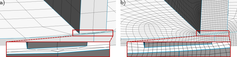
Figure 3: Focus on a small CAD feature of the Block model. Without adaptation of the size map (a), there are low quality elements around the small feature. With size map adaptation (b), there are small high-quality elements around the feature and irregular vertices to make the transition to coarser regions.

4.2 Global size map

To build a global continuous and smooth size map $s(\mathbf{x})$, we combine the minimal size field $s^{min}(\mathbf{x})$ with the size maps $s_{i}^{cf}(\mathbf{x})$ associated to the cross field conformal scaling (Sec. 3.3) computed on each CAD face $\mathcal{S}_{i}$.

The conformal scaling fields (Sec. 3.3) are defined up to a constant $C_{i}$ that can be tuned in order to have $N_{i}$ quads on the surface $\mathcal{S}_{i}$. Starting from a global target number of quads $N$, we distribute the quads on each CAD face based on their areas, i.e. $N_{i}=\frac{\text{area}_{i}}{\text{total area}}N$. Another advantage of this simple approach is that we can easily take user preferences into account. If a user want a specific number of quads on a CAD face, we can use this value instead of the one proportional to the area.

The conformal scaling size maps are not continuous at the CAD interfaces. Consider a point $\mathbf{x}$ on a CAD curve common to the faces $\mathcal{S}_{i}$ and $\mathcal{S}_{j}$, we have $s_{i}^{cf}(\mathbf{x})\neq s_{j}^{cf}(\mathbf{x})$ because the cross field gradients, and thus the conformal scaling, are not equal on both sides of the curve. To make a continuous and smooth union of the $s_{i}^{cf}$ fields in a global one $s^{cf}$, we apply a similar smoothing process as before (Sec. 4.1). Initialize the union of the size map, taking the minimum on the shared vertices (CAD corners and curves): $s^{cf}(\mathbf{x})=\min_{i}(s_{i}^{cf}(\mathbf{x}))$. Then apply a one-way smoothing (Eq. 10) with the maximal gradient $g_{max}$.

To blend the small feature size map and the conformal scaling, we simply take the minimum everywhere:

$$s(\mathbf{x})=\min(s^{cf}(\mathbf{x}),s^{min}(\mathbf{x}))$$

A local example of our size map taking the small CAD features into account is shown on Fig. 3, where small quads are used in the region where two feature curves are close to each other. This figure is a zoom on a small part of the larger Block model (Fig. 9), which have lot of small features and where significant size map transitions are necessary in many regions.

4.3 Curve quantization

We call quantization the process of going from continuous fields (cross field, size map) to a quadrilateral mesh which is characterized by discrete quantities, such as the number of points on a model curve or the number of quads in a model face. As we are following the robust Gmsh’s “surface to volume” philosophy, the curve quantization is important in our pipeline.

The process of first meshing the model curves then the model surfaces, constrained to the curve discretization, works well for the generation of triangulations (or tetrahedrizations) but it is not optimal for quadrilateral meshing (or hexahedral meshing) as the quad topological constraints (chords) are global and go through the model curves. For instance, imagine a simple rectangular face for which the ideal edge numbers, according to the continuous cross field induced size map, are $[9.4,4.1,10.6,3.9]$ on the four sides. A simple quantization by integer rounding would choose respectively $[9,4,11,4]$ edges. While a quadrilateral mesh with this quantization exists, it is not structured as it must include one pair of +1/–1 irregular vertices to make the transition from $9$ edges on one side to $11$ edges on the opposite side.

Finding a good curve quantization for quad meshing, for a generic CAD model with CAD faces of arbitrary topology, is a complicated and totally open problem, which has been mostly ignored in the literature. If we restrict ourselves to quadrilateral CAD faces (with T-junctions), there is the global quantization in [14], but in our case we do not have such quadrilateral layout.

For the current paper, our quantization of CAD curves remains quite simple. We use the integer-rounded value of the ideal number of edges computed by integrating the global size map (Sec. 4.2), except for curves which are on quadrilateral CAD faces, where we impose equality on the opposite sides. This non-optimal quantization leads to many necessary dipoles (pair of +1/–1 irregular vertices) in the final quad meshes of the different CAD faces. Eliminating them requires to change the CAD curve 1D meshes, which is out of the scope of the current paper.

Size map integration on curves

Consider a CAD curve $\mathcal{C}$ parametrized by $t$ varying from $a$ to $b$. The floating-point number of edges on the curve according the size map is: $\bar{n}_{e}=\int_{a}^{b}dl/s(\mathbf{x})$ with $dl=\left\lVert x^{\prime}(t)\right\rVert dt$. To get a integer number of edges $n_{e}$, we use a simple rounding: $n_{e}=\text{round}(\bar{n}_{e})$. The parameter $t_{i},i\in[1,n_{e}-1]$ associated to the $i$-th interior point of the curve is such that:

$$\int_{a}^{t_{i}}\frac{dx}{s(\mathbf{x})}=\frac{i}{n_{e}}\int_{a}^{b}\frac{dl}{s(\mathbf{x})}$$ (11)

This integral equation can be solved via numerical integration, by adding values along the curves until the sum is equal to $i\bar{n}_{e}/n_{e}$, with linear interpolation between the samples.

To mesh the curve $\mathcal{C}$, we compute the vertex positions $\mathbf{x}_{i},i\in[1,n_{e}-1]$ by computing the parameters $t_{i}$ with (Eq. 11) and evaluating the CAD curve parametrization: $\mathbf{x}_{i}=f(t_{i})$. With this approach, the points are well placed on the curves according to the size map, making smooth transitions from the small CAD feature regions to the coarser ones, where smaller but useful variations come from the cross field conformal scaling.

Topological constraints on quadrilateral patches

Integrating the size map does not take into account the particularities of quad mesh topology, such that the quads are organized in topological chords (dual loops of adjacent elements). In this work, we adjust the number of edges $n_{e}$ on the opposite sides of quadrilateral CAD faces.

Consider a CAD face whose boundary is made of four CAD curves $(\mathcal{C}_{1},\mathcal{C}_{2},\mathcal{C}_{3},\mathcal{C}_{4})$, we force the number of points to be equal on the opposite edges, i.e. $n_{e1}=n_{e3}$ and $n_{e2}=n_{e4}$, except if the integrated values are very different. When two adjacent quadrilateral CAD faces share a curve $\mathcal{C}_{c}$, the value $n_{ec}$ must be the same on both faces. This means the equality constraints propagate in the CAD model. To resolve the propagation, we build the topological chords associated to the quadrilateral CAD faces. A chord is made of topologically parallel CAD curves, which all receive the same fixed number of points, that we compute by averaging the ideal values previously computed on each curve.

With this simple propagation, the chords propagate only if two adjacent quadrilateral faces share a single curve which is one of their four sides. We do not propagate across T-junctions. Our quantization applies only on the connected subsets of conformal quadrilateral patches of the CAD model. Dealing with T-junctions is more complicated and corresponds to the quantization phase of [14], for which there is not always a solution (Sec. 2).

5 Unstructured frontal quadrilateral mesh generation

Now that the 1D meshes of the CAD curves have been generated, it’s time to move to the initial quad-meshing of the CAD surfaces. The all-quad mesh is generated by following a robust three step approach: (1) generate a triangulation with right-angle triangles using the methodology in [38], (2) combine some triangles into quads to form a quad-dominant mesh and (3) apply midpoint subdivision to produce an all-quad mesh. We also describe the geometry smoothing and untangling techniques (Sec. 5.3) which are used extensively in our pipeline.

5.1 Frontal point insertion

A scaled cross field ${\bf f}(\mathbf{x})$ has been generated where the size of the crosses is the global size map $s(\mathbf{x})$ (Sec. 4.2). Mesh vertices are created on every face $\mathcal{S}$ in a frontal fashion, starting from its boundary $\partial\mathcal{S}$. Vertices of $\partial\mathcal{S}$ are added in a priority queue. Vertex $\mathbf{x}$ at the top of the queue tries to add four new vertices in the domain in the 4 directions of the local cross field $f(\mathbf{x})$ and at a distance $s(\mathbf{x})$. New vertices are only added (i) if they lie inside $\mathcal{S}$ and (ii) if they are not to close to any existing vertex. When a vertex is successfully added, it is inserted at the end of the queue and the procedure continues until no new vertices can be generated. The points are iteratively inserted in the triangulation with a Delaunay kernel, as described in [38]. This mesher is close to classic frontral Delaunay triangular meshing [36], except that the goal is to build right-angled triangles in agreement with the cross field.

5.2 Quad combination and midpoint subdivision

The triangulation is transformed into a quad-dominant by combining pairs of triangles into quads. As triangles are allowed, there is no need for advanced matching technique such as Blossom-Quad [37] and we simply use a greedy selection. All the merge candidates (two triangles $\to$ one quad) are computed and sorted by the geometric quality (Sec. 5.3) of the resulting quads, weighted by the alignment with the cross-field. Then the quads are iteratively selected, as long as their quality is superior to a minimal threshold (SICN $>0.1$ in our case).

The all-quad mesh is obtained by subdividing all quads into four sub-quads and all triangles into three sub-quads. This subdivision is called midpoint subdivision and is topologically equivalent to the Catmull–Clark subdivision surface technique. New vertices are added at the centers of each edge and each element.

To accurately represent the CAD model geometry, it is best to project the new midpoint vertices on the CAD curves and faces. However, this projection is not robust in the sense that it may create invalid quads (negative quality). This difficulty is similar to the one faced when doing CAD snapping for high-order meshing, and is not easy to solve. In our pipeline, we iteratively try to snap all midpoint vertices while monitoring the quality of the adjacent elements, and we revert the projections which lead to negative elements. Even if rejected projections are rare and definitively not ideal, this check is necessary to ensure the geometric validity of the final mesh when dealing with complex CAD models. For better geometric fidelity, one could decrease the size map locally to better capture the geometry and restart the meshing process of the CAD curves and surfaces in the neighborhood.

An example of quad mesh produced by this procedure is shown in Fig. 2.2.b. It is actually a fairly good unstructured all-quad mesh, yet containing an excessive number of irregular vertices.

5.3 Geometry optimization

Geometrical smoothing of a mesh is the process of finding good vertex positions given a fixed mesh topology. Ideally, we would like the positions to maximize some quality functional, but such formulation are usually too expensive to be solved globally and we have to resort to more efficient techniques. Smoothing of unstructured quadrilateral meshes is still a challenging problem in our opinion. Simple and fast techniques, such as Laplacian smoothing and its variants, often produce tangled elements (negative quality) while more advanced non-linear optimization techniques are computationally too expensive to be used on large sets of elements. For CAD surfaces, an additional expensive operation is the projection of a 3D point on the surface, which is typically performed many times during optimization. As an approximation, it is possible to project on a triangulated representation of the geometry, but even this approximation is expensive when applied millions of times.

In this work, we apply a great deal of topological remeshing (Sec. 6) and each time we use smoothing techniques to determine the geometry before validating or rejecting the remeshing. Concretely, this means that we are applying smoothing all the time, on many more elements that there are in the initial or final mesh. For instance, if there are $100k$ vertices in the quadrilateral mesh, we will probably smooth millions of vertex positions. While smoothing is always expensive in any mesher, the computational cost is particularly critical in our approach and we have to employ fast techniques and fall-back to expensive ones only locally and in last resort. Before and after any smoothing operation, we compute the element qualities and we revert the vertex positions if the quality decreased.

Quality metric

For consistency with other Gmsh algorithms, we use the Signed Inverse Condition Number (SICN) metric to evaluate the geometric quality of the quads. It is the inverse of the condition number in Frobenius norm of the mapping from the quad to the regular square. This metric, which is also called shape quality [40], has a behavior similar to the scaled Jacobian: the range is $[-1,1]$ with negative values for invalid elements and a maximum value of $1$ for squares (and rectangles for the scaled Jacobian). As with the Jacobian, the SICN value is not constant inside a quad, so we use the minimum. In practice, most mesher sample the quad quality at the four corners and take the minimum. Assuming the quad corners are $\mathbf{x}_{i},i\in[1,4]$ and $N_{i}$ are the CAD surface unit normals, the scaled Jacobian and SICN values at the i-th corner are respectively [40]:

$$SJ_{i}=\frac{\mathbf{L}_{i-1}\times\mathbf{L}_{i}}{\left\lVert\mathbf{L}_{i-1}\right\rVert\left\lVert\mathbf{L}_{i}\right\rVert}\cdot\mathbf{N}_{i},\quad SICN_{i}=2\frac{\mathbf{L}_{i-1}\times\mathbf{L}_{i}}{\left\lVert\mathbf{L}_{i-1}\right\rVert^{2}+\left\lVert\mathbf{L}_{i}\right\rVert^{2}}\cdot\mathbf{N}_{i},\;\text{ with }\mathbf{L}_{i}=\mathbf{x}_{i+1}-\mathbf{x}_{i}$$ (12)

When one edge length $\left\lVert\mathbf{L}_{i}\right\rVert$ tends to zero (geometrical edge collapse), the scaled Jacobian will not tend to zero but to the sine of the angle at the corner (as $\mathbf{L}_{i-1}\times\mathbf{L}_{i}=\left\lVert\mathbf{L}_{i-1}\right\rVert\left\lVert\mathbf{L}_{i}\right\rVert\sin(\theta)\ \mathbf{n}$). This observation have very practical implications: when sampling the quality at the four corners, a quad mesh may have many almost-collapsed edges (e.g. $1e^{-12}$) but still a high minimum scaled jacobian (e.g. $0.7$). On the other hand, the SICN quality metric, also sampled at the four corners, will tend to zero with edge collapse. In our experience, the discretized SICN should be preferred to the scaled Jacobian when evaluating the quality of isotropic quadrilateral meshes.

Laplacian smoothing in CAD parameter domain

When we are dealing with a parametrized CAD model, we have a valid $uv$ trimmed parametrization of each CAD face. To smooth the vertices inside a cavity $C$, which can be a whole CAD face, we extract continuous $\mathbf{uv}\in\mathbb{R}^{2}$ values for each boundary $\mathbf{x}\in\partial C$. One must be careful with the parametrization jumps (e.g. periodic seam on a cylinder). Sometimes it is not possible to have a continuous boundary in the parameter domain (e.g. around the pole of a sphere parametrization), and we move to the next smoothing options. Once we have a continuous $\mathbf{uv}$ on the boundary, we simply solve the unweighted Laplacian equations $\Delta u=0$ and $\Delta v=0$, where each internal value is the arithmetic average of its edge-connected neighbors. It is important to use the arithmetic average and a direct linear solver to respect the maximum principle and avoid inverted elements in the parameter domain. Depending on the distortions in the CAD parametrization, this technique may both produce high-quality or poor elements. To retrieve the 3D positions, we then apply the CAD face mapping $\mathbf{x}=f(\mathbf{uv})$. Depending on the resulting element qualities, we keep or we reject this smoothing. The huge advantage of this approach is that there is no surface projection and simply two linear solves, making it a very fast smoother. Even if the quality may be poor due to distortion in the CAD mapping, it is still a good initial guess since all elements are usually untangled.

FDM Winslow kernel on regular vertices

Winslow smoothing [48] is the industry-standard technique used for structured grid mesh generation [42]. Given a fixed boundary, the idea is to solve the Winslow non-linear elliptic PDE $\Delta_{x}\mathbf{u}=\mathbf{0}$, where $\mathbf{u}(\mathbf{x})$ are the coordinates in a certain computational space and $\mathbf{x}$ are the coordinates in the physical space. The advantage of this approach is that the two coordinate components are coupled and the resulting quads are nicely shaped, with some orthogonality enforced even under large distortions. By applying a finite difference (FDM) discretization to the Winslow equation [22], we can derive a local smoothing kernel for regular vertices in the quadrilateral mesh. Assuming that $(\mathbf{x}_{1},...,\mathbf{x}_{8})$ are the ordered vertices of the stencil around the regular vertex $\mathbf{x}$, its new position is given by:

$$\begin{split}\alpha_{0}(\mathbf{x}_{1}+\mathbf{x}_{5}-2\mathbf{x})+\alpha_{1}(\mathbf{x}_{3}&+\mathbf{x}_{7}2\mathbf{x})-\frac{1}{2}\beta(\mathbf{x}_{2}+\mathbf{x}_{6}-\mathbf{x}_{4}-\mathbf{x}_{8})=0\\ \text{with }\alpha_{0}=(\mathbf{x}_{3}-\mathbf{x}_{7})\cdot&(\mathbf{x}_{3}-\mathbf{x}_{7}),\quad\alpha_{1}=(\mathbf{x}_{1}-\mathbf{x}_{5})\cdot(\mathbf{x}_{1}-\mathbf{x}_{5}),\quad\beta=(\mathbf{x}_{1}-\mathbf{x}_{5})\cdot(\mathbf{x}_{3}-\mathbf{x}_{7})\end{split}$$ (13)

This smoothing is moving the vertex outside of the CAD surface. We project back on it by finding the closest point on a triangulated representation of the CAD surface (with a kd-tree for faster spatial queries). If we want a more accurate projection, such as in the last steps of the smoothing, we ask the projection to the CAD geometric kernel, which in our case is OpenCASCADE.

Angle-based kernel on irregular vertices

On irregular vertices, we use the angle-based smoothing kernel of [1], where the idea is to move the vertices on the bisector of the one-ring. As the above Winslow kernel, it works well in regions where the mesh is not too constrained but it may create inverted elements in complex configurations. An alternative for irregular vertices is the unstructured Winslow FDM kernel [22], but it is more complicated and would suffer from the same issues.

Smoothing loop

The smoothing kernels, followed by projection on the CAD, are applied iteratively to all vertices of the current cavity, until the displacement is smaller than a criteria or the maximal number of iterations is reached. This iterative process is slower than the uv-Laplacian smoothing, because of the non-linearity of the kernel and of the surface projections, so we generally use it without waiting for convergence. It should be notated that these kernels may produce tangled elements, especially close to concave CAD features or in very irregular regions. For this reason, we compare the element qualities before and after, and roll back if necessary.

Non-linear optimization

Some local configurations are difficult to untangle and smooth, or even impossible. This is generally due to a mix of constraining CAD features and mesh irregularity, such as for the disk quadrangulation remeshing (Sec. 6.3). In these tricky situations, we use the non-linear untangler of Mesquite [10] on very small patches of quads. This optimization can fail or may convergence too slowly, so in practice we use a time limit of $1$s. Failure to untangle is not a big issue in our pipeline because we start from a geometrically valid unstructured mesh by construction, so untangling is only encountered during remeshing and we can simply rollback if the result is tangled.

6 Topological quadrilateral meshing

Unstructured quadrilateral meshes generated frontally (Sec. 5) typically have a large excess of irregular vertices (e.g. Fig. 1.c.). To transform the mesh into a quasi-structured quad mesh (e.g. Fig. 1.d.), we need to remove most of the irregular vertices while preserving the ones that important to accommodate the model topology and geometry. We achieve this topological improvement by extracting cavities of quads in the unstructured mesh and by replacing them by more regular quad meshes. We act at three different scales: the cavity may be an entire CAD face when it is topologically simple (Sec. 6.1), the cavity may be a convex patch of quads in a CAD face (Sec. 6.2), or the cavity may contain only the quads adjacent to a vertex (Sec. 6.3). For large cavities (Sec. 6.1 and Sec. 6.2), we look for replacement meshes in a list of high-quality predefined patterns (Fig. 4). For local cavities, we look for replacements in the list of all possible disk quadrangulations (Sec. 6.3).

Each time we apply a topological operation (meshing or local remeshing), it is very important to verify that the geometric quality of the mesh is satisfactory. We always apply the geometric smoothing techniques defined in Sec. 5.3. If the geometry is invalid, or if the quality decreased too much compared to the initial configuration after remeshing, we cancel the mesh replacement.

Common definitions

A cavity $C$ is a set of quads forming a simply-connected part of the mesh. The boundary of a cavity $\partial C$ is a closed polyline. Consider a vertex $\mathbf{x}\in\partial C$. Let us call $n_{\mathbf{x}}$ the number of quads adjacent to $\mathbf{x}$, which are also the quadrilateral valences. We distinguish $n^{in}_{\mathbf{x}}$ the number of quads adjacent to $\mathbf{x}$ that belong to $C$ and $n^{out}_{\mathbf{x}}$ the number of quads adjacent to $\mathbf{x}$ that do not belong to $C$. We have $n_{\mathbf{x}}=n^{in}_{\mathbf{x}}+n^{out}_{\mathbf{x}}$. It should be noted that we usually only consider the quads in the current CAD face $\mathcal{S}$, not the global quadrilateral mesh of the model.

The vertex $\mathbf{x}\in\partial C$ is a convex corner of the cavity if and only if $n^{in}_{\mathbf{x}}=1$. It is a concave corner of the cavity if the vertex is strictly inside the CAD face, $\mathbf{x}\notin\partial\mathcal{S}$, and if $n^{out}=1$.

By splitting the cavity boundary $\partial C$ at the convex and concave corners, we form $m$ regular sides, which respectively contain $N_{1},...,N_{m}$ edges.

6.1 Pattern-based quadrilateral meshing

Given a cavity with $m$ sides (containing $N_{1},..,N_{m}$ edges), it is often (not always) possible to topologically find a quadrilateral mesh to fill the interior from a list of predefined patterns (Sec. 6.1.1). Such quadrilateral meshes (Fig. 4 bottom) are the anisotropic subdivision of coarse quadrilateral meshes (Fig. 4 top). By anisotropic subdivision, we mean that each topological chord (dashed lines in Fig. 4) can be subdivided independently of the others. We use this constrained topological approach to mesh whole CAD faces when their topology is simple (Sec. 6.1.2), skipping the frontal unstructured mesher, or to iteratively improve patches of quads in the initially unstructured mesh of a CAD face.

6.1.1 Matching patterns

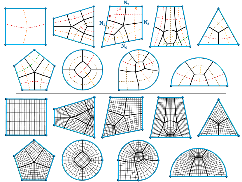
Figure 4: Pattern-based topological quad meshing. The patterns are defined by coarse quadrilateral meshes (top). The topological chords (dashed lines) can be subdivided independently to build refined quadrilateral meshes (bottom).

Consider the cavity with side edges $(N_{1},...,N_{m})$, we check if there is a matching with a quad pattern with $m$ sides in our pre-computed pattern list (e.g. Fig. 4). For each pattern $\mathcal{P}$, we denote $(s_{1},...,s_{c})$ the number of edge subdivision of the $c$ topological chords of the patterns (dashed lines Fig. 4). There is a quadrilateral mesh if it possible to find strictly positive chord subdivisions $s_{j}>0,j\in[1,c]$ such that on each side, the sum of the subdivisions of the chords included in the side is equal to the side number of edges:

$$\forall i\in[1,m],\quad\sum_{j\in[1,c]}w_{ij}\;s_{j}=N_{i}$$ (14)

where $w_{ij}$ is the number of times the chord $j$ in inside the side $i$. In practice, $w_{ij}$ is equal to $0$ (the chord is not on the side), $1$ (the chord go through the pattern) or $2$ (the chord starts and finish on the side, turning inside). This linear system may be undetermined if there are more chords (columns) than sides (rows). We are not only interested in a solution to the linear system, we want one that is integer and strictly positive because it corresponds to the chord subdivisions of the pattern. We also want the values to be well balanced so the output quadrilateral mesh is not highly distorted. This behavior can be obtained by finding the solution that is the closest to an ideal subdivision of the chords, defined by equi-balancing the values on each side. This corresponds to a non-linear objective function where we minimize a distance, e.g. $E=\sum_{j}{(s_{j}-x_{j})^{2}}$ with $x_{j}$ the ideal subdivisions.

To solve such system, with linear constraints and a quadratic objective function, the ideal approach is to use a suited Mixed-Integer solver. From a practical point of view, such solvers are large software dependencies and would be overkill for our problem. As our system is usually very small, we have adopted a much simpler solution: compute the integer row echelon form of the system matrix, start from an ideal guess (by balancing the values) and use a depth-first search to find a solution satisfying all the constraints by rolling up in the echelon form matrix. However, even if the system is small, the exhaustive search that happens when there is no solution is too slow for practical use. So we abandon the search after a few hundred attempts. While this approach may sound naive, we observe that it works well in practice as the solution, if there is one, is close to the ideal subdivisions (initial guess). It should be noted that when looking for match with a pattern, one must check all the rotations of the sides $[N_{1},...,N_{n}]$, clockwise and counter-clockwise.

The advantage of this integer formulation is that it is generic and works on any quadrilateral pattern. The user can add a new pattern by simply specifying the coarse quadrilateral mesh. The construction of the sides, chords and linear systems are all handled automatically. While it is possible to construct thousands of patterns by enumerating the quadrangulations of the disk (Sec. 6.3), it should be noted that most of them do not lead to high-quality quadrilateral meshes. For this reason, we restrict ourselves to the patterns of Fig. 4 that we selected manually.

For a practical example, consider a rectangular CAD face with respectively $[N_{1},N_{2},N_{3},N_{4}]$ edges on its sides. It can potentially match with the first four patterns of Fig. 4. For the first pattern, the condition is obviously equality of the subdivisions on the opposite sides ($N_{1}=N_{3}$ and $N_{2}=N_{4}$). Let consider a more interesting case: the third pattern. The sum of the chord subdivisions on each side gives the system:

$$a+b+c =N_{1}$$

$$d+e =N_{2}$$

$$a+c =N_{3}$$

$$b+d+e =N_{4}$$

We can see that $b$ must respect $b=N_{3}-N_{1}$ and $b=N_{4}-N_{2}$, which is a quite natural condition if we look at the dual chords (Fig. 4). On the other hand, there is no solution for this pattern if $N_{3}-N_{1}\neq N_{4}-N_{2}$. Assuming the above condition is respected, the balance between the respective subdivisions $a,c$ and $d,e$ are left to the minimization of the objective function, or to the depth-first search with our technique.

Related work

The above integer formulation is not new and has been introduced for patterns with a single interior vertex in [11]. A general ILP formulation for more complicated patterns has been developed in [41] and is equivalent to ours (Eq. 14).

Geometry

The integer formulation is purely topological and does not take geometry into account. A very interesting extension would be to find a way to incorporate geometric information from the cavity boundary into the objective function, in order to find optimal chord subdivisions. In our pipeline, the mesh geometry is obtained by smoothing (Sec. 5.3) with a fixed boundary, and the new quadrilateral mesh is only kept if its quality is better than the initial one.

6.1.2 Application to simple CAD face meshing

In a complicated CAD model (e.g. Fig. 9), there are usually lot of CAD faces but many of them have the topology of simple polygons (e.g. triangles, rectangles, pentagons). Given such polygon and the number of edges on each of its sides, it is often possible to directly find a quadrilateral mesh with our topological matching technique (Sec. 6.1.1).

In practice, we loop over all CAD faces and check if they have the same topology ($\chi$ and convex corners) as some of our patterns. When the topology is identical, we search for a subdivision of the pattern which matches the number of edges on each side of the CAD face, previously determined by the curve quantization step (Sec. 4.3). This matching exists if there is a strictly positive solution to the integer linear problem (Eq. 14). Once the quadrilateral mesh topology is determined, we can find the vertex positions by employing our quad mesh geometry smoother (Sec. 5.3). We only keep the quad mesh only if the geometric quality is satisfactory, and if it is not we fall back to the unstructured approach.

Examples

To see the usefulness of this pattern-based pre-meshing in real-life situations, we can look at the results on two CAD models. The A319 model is made of 83 CAD faces, 275 CAD curves and 287 CAD corners and the Block model is made of 533 CAD faces, 1584 CAD curves and 1044 CAD corners. After the curve meshing (Sec. 4.3), we apply our pattern-matching on all CAD faces and we are able to directly build the quadrilateral meshes of respectively $75/83$ and $419/533$ CAD faces, as shown in Fig. 5. These results are very interesting because it means that we are able to build high quality meshes on most of the simple CAD faces in a short amount time, for which there is no need to use more computationally expensive techniques.

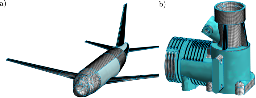
Figure 5: Pattern-based quadrilateral meshes of $75/83$ CAD faces on the A319 model (a) and $419/533$ CAD faces on the Block model (b).

6.2 Quasi-structured topology with cavity remeshing

On the remaining CAD faces, we start from the unstructured quadrilateral mesh (Sec. 5) and we improve its topology by locally remeshing cavities with the pattern-matching technique (Sec. 6.1). Our objective is to iteratively reduce the number of irregular vertices in order to reach a quasi-structured topology. Consider a CAD face, there are four sources of irregular vertices: (i) the face topology (see Eq. 2), (ii) the face geometry, (iii) the non-ideal quantization of the curves (Sec. 4.3) and (iv) the non-ideal behavior of the frontal mesher (frontal collisions, size map not adapted to CAD features or cross field gradients, etc). The irregular vertices from (i) and (ii) are captured as cross field singularities (including the ones we artificially added at acute corners). In the current paper, we work on removing the irregular vertices (iv) caused by the unstructured quadrilateral mesher, while preserving the irregular vertices (i) and (ii) which are necessary to have a good quadrilateral mesh in the end. It should be noted that the irregular vertices (iii) caused by the non-ideal quantization cannot be removed by considering only one CAD face, but the whole model quadrilateral mesh should be taken into account. We leave this last improvement for future work as it is definitively not trivial: the global quadrilateral mesh is potentially non-manifold (e.g. multiple volumes) and the CAD features must be strictly preserved while applying global operations across multiple CAD faces.

To remove the unnecessary irregular vertices, we build convex topological cavities in the quadrilateral mesh, which contains three or more irregular vertices, and we replace them by more regular quad meshes (the patterns defined in Sec. 6.1). This process is illustrated on Fig. 6, where a pentagonal cavity with five valence $3$ ($k=1$) and six valence $5$ ($k=-1$) irregular vertices ($\sum k=-1$) is replaced by a pentagonal patch with only one valence 5 irregular vertex ($k=-1$). The key to our approach is to not apply this process blindly but in a specific way to preserve the irregular vertices matching cross field singularities.

The idea of remeshing cavities with more regular patterns is not new [11, 41] and has been exploited in quad meshing [45, 26, 44]. The difficulty is in choosing which cavities to remesh, because uncontrolled greedy remeshing will remove irregular vertices that were important for mesh quality, leading to highly distorted meshes. For instance, a rectangular cavity may eliminate a valence three singularity close to a convex CAD curve and a valence five singularity close to a concave CAD curve, which were both useful irregular vertices used to accommodate the model geometry.

We call singularities the irregular vertices that we preserve, which mainly come from the cross field singularities, and we call unnecessary irregular vertices the ones we want to eliminate. The singularities are used to control and constrain the growth of the remeshable cavities that absorb the unnecessary irregular vertices.

6.2.1 Growing remeshable cavities

To iteratively improve the mesh of a CAD face $\mathcal{S}$, we grow convex cavities (patch of quads) and replace them. To grow a convex cavity $C$, we start from an initial simply connected set of quads $C_{0}$ (e.g. quads adjacent to a vertex) and we iteratively add quads adjacent to the cavity. To ensure the convexity of the cavity, if one of the vertex $\mathbf{x}$ on the boundary $\partial C$ is concave, e.g. $\mathbf{x}\notin\partial\mathcal{S}$ and $n_{\mathbf{x}}^{\text{out}}=1$, we add the adjacent exterior quad in priority. During the growth, we also ensure that (i) a singularity (flagged irregular vertex to preserve) is never added to the interior of the cavity and (ii) a CAD concave corner is never fully surrounded by the cavity ($\mathbf{x}$ concave CAD corner, $n_{\mathbf{x}}^{\text{out}}=0$). This process is illustrated in Fig. 6, where a pentagonal cavity is growing starting from a valence-5 singularity. Each time the growing cavity is convex and has absorbed new irregular vertices, we check if it is remeshable by solving the matching problem (Sec. 6.1.1) with the target replacement patterns. If it is remeshable, we store it as the last remeshable cavity. We either stop if we want a minimal cavity, or we continue the growth if we want a maximal cavity.

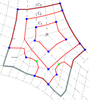
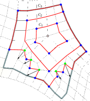
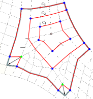
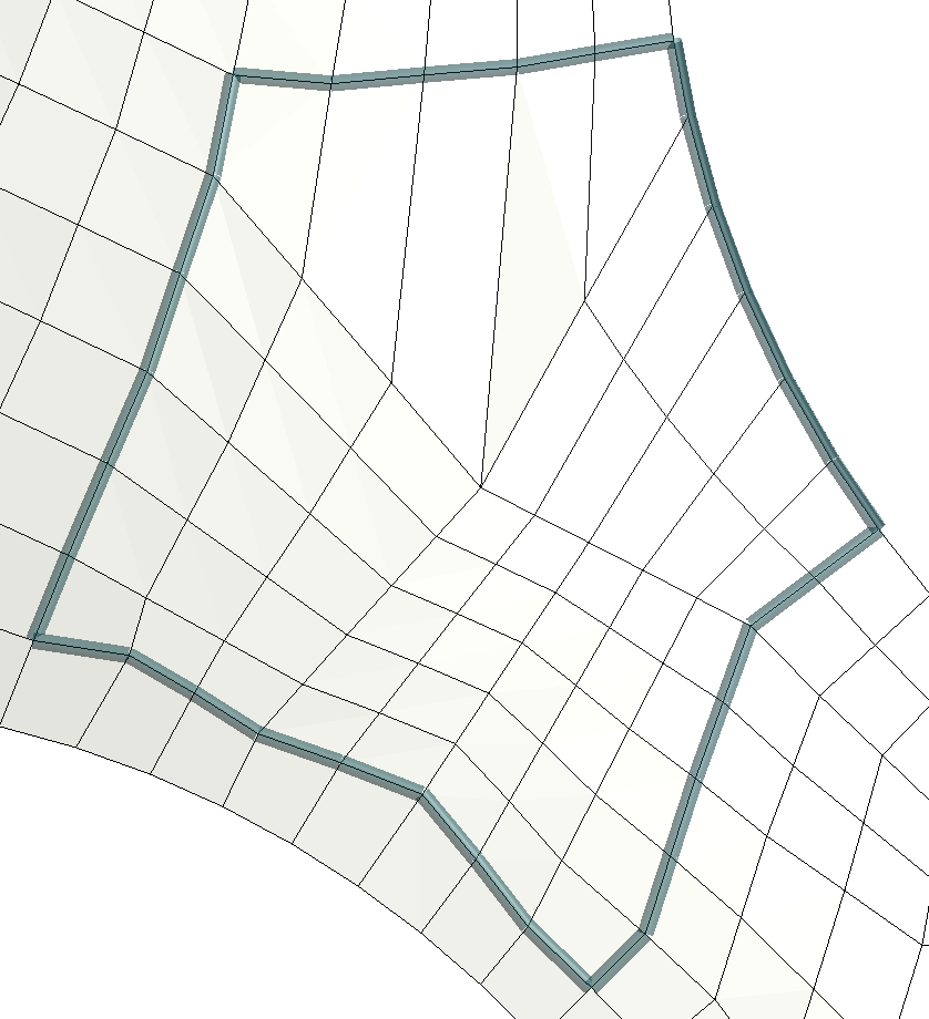
(a)	(b)	(c)	(d)

Figure 6: Growing a cavity around one vertex of index $-1$ (in pink). Convex corners are in blue and concave corners are in green. The remeshed cavity (d) has one irregular vertex instead of eleven.

6.2.2 Cavity remeshing strategy

The choice of cavity seeds and the order in which cavities are grown and remeshed matters. When a triangular or a pentagonal cavity built around a singularity is remeshed, removing pairs of $+1/-1$ irregular vertices, it produces quads with only one irregular vertex (associated to the initial singularity), but the new singularity topological position is translated compared to the initial one. On Fig. 6.d., we can observe that the new irregular vertex is moved closer to the top side (distance of one edge instead of three initially). Another way to interpret this is that when a pair of $+1/-1$ irregular vertices is eliminated via a singularity, it will attract it or push it away, depending of the pair orientation and the singularity index. This behavior has important consequences: if a mesh singularity is used a lot to absorb all other irregular vertices, it may end up far away from the initial cross field singularity, leading to important distortions in the mesh geometry. So in order to produce a high-quality quasi-structured mesh, we must adopt a cavity remeshing strategy that will minimize the movements of the singular vertices and keep them close to their initial position in the cross field.

On a given CAD face $\mathcal{S}$, we apply the following steps as long as there is improvement (i.e. in a while loop):

1. Starting from unnecessary irregular vertices, grow and remesh maximal rectangular cavities that do not contain singularities and that match the regular grid pattern (first one on Fig. 4). The goal is to eliminate the opposed irregular $+1/-1$ pairs without distorting the mesh.

2. Starting from the singularities (index $k=+1$ or $k=-1$), grow and remesh minimal triangular or pentagonal cavities that contain the starting singularity and the non-zero minimum number of unnecessary irregular vertices while keeping the target index (i.e. $\sum k=-1\text{ or }+1$). The goal is to eliminate the irregular vertices while distributing the mesh distortion on all the singularities.

3. Re-apply Step 1, in case some new regular cavities have been unlocked by the previous step.

4. Starting from unnecessary irregular vertices, grow and remesh minimal rectangular cavities that do not contain singularities and that match one of the four rectangular patterns of Fig. 4. The goal is to enable size transitions in the mesh while reducing the number of irregular vertex pairs. To avoid large geometric distortions, we use minimal remeshable cavities and we verify that the mesh quality is not degraded too much after smoothing.

This process is the core of our quasi-structured topological improvement. Fig. 2.2. illustrates the absorption of irregular vertices by the cross singularities. For a more complicated example, we can look at the Block model illustrated in Fig. 9, where the zooms show the kind of mesh size transitions which are produced by the rectangular pattern cavity remeshing.

6.3 Local remeshing with disk quadrangulations

Unstructured quad meshes constructed in an indirect fashion may contain a few very irregular vertices, that we call defects. The goal of this local remeshing is to eliminate them before applying the larger cavity remeshing (Sec. 6.2). In the interior of a CAD face, we say that a vertex is very irregular if its quadrilateral valence is more than 6, i.e. its index is $k\leq-2$. On the CAD curves, we say that a vertex is a defect if its valence is different from two on the adjacent CAD faces. On CAD corners, we want to enforce the ideal valence which is deduced from the associated angle in the CAD faces, e.g. valence three for a concave $270^{\circ}$ corner. We can also enforce user-prescribed corner valences with this technique, which can be useful when hand-crafting boundary layers for specific applications. The goal of the local remeshing step is to eliminate the defects (valence different from the allowed range) by changing the topology locally.

When forming a cavity with the quads adjacent to a vertex, we are building a topological disk. We can replace the interior of the cavity with any quadrilateral mesh as long as we do not change the cavity boundary, which is a closed polyline. Our idea is simple: browse all the possible disk quadrangulations (Sec. 6.3.1) and use the best one, according to a quality criterion (Sec. 6.3.2). An example of elimination of a valence six vertices is shown on Fig. 8.

6.3.1 Quadrangulations of the disk

Figure 7: All quadrangulations of the disk bounded by $4$, $6$, $8$, $10$ and $12$ vertices with $0$, $1$, $2$, $3$ and $4$ internal vertices.

The exhaustive list of disk quadrangulations can be built by recursively applying the three edge flips that add a quad to a current quadrangulation, starting initially from a single quad. This is a simple 2D version of the algorithm used to build shellable hexahedral meshes of the sphere in [43]. Our implementation is open-source . The only technical difficulty is in detecting equivalent quadrilateral meshes that have different vertex ordering. For this we use the open-source library Nauty [28] to compute the canonical labeling of the edge graphs. In our meshing software, we only store the list of the disk quadrangulations up to a certain size in a large table.

For practical meshing, the only disk quadrangulations that are interesting are the ones with valence three, four, five inside (indices $1,0,-1$) and valences one, two, three on the boundary (indices $1,0,-1$). On Fig. 7, we show the disk quadrangulations with up to $12$ vertices on the boundary and up to $4$ vertices in the interior. These configurations are more general that the patterns previously used (Sec. 6.2) because they include concave vertices on the cavity boundary.

6.3.2 Local remeshing

Consider a cavity $C$ that we want to remesh, with its boundary $\partial C$ defined by the polyline $[\mathbf{x}_{1},...,\mathbf{x}_{b}]$. We want to select the best replacement in the list of disk quadrangulations with $b$ vertices on the boundary, including all rotations clockwise and counter-clockwise of the patterns. As the cavity is immersed in a larger quadrilateral mesh, the quadrilateral valence outside the cavity associated to each vertex of $\partial C$ is fixed: $[n_{\mathbf{x}_{1}}^{\text{out}},...,n_{\mathbf{x}_{b}}^{\text{out}}]$. The future quad valences inside the cavity $[n_{\mathbf{x}_{1}}^{\text{in}},...,n_{\mathbf{x}_{b}}^{\text{in}}]$ are parameters of each disk quadrangulation. We also know the ideal valences $[\bar{n}_{\mathbf{x}_{1}},...,\bar{n}_{\mathbf{x}_{b}}]$ in the global quadrilateral mesh according to their position in the CAD face, e.g. $\bar{n}_{\mathbf{x}_{j}}=4$ inside if regular, $\bar{n}_{\mathbf{x}_{j}}=2$ on a curve, $\bar{n}_{\mathbf{x}_{j}}=3$ on a concave corner.

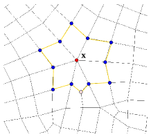
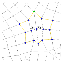
Figure 8: Removing a very irregular vertex $\mathbf{x}$ (in red) of index $k=-2$. Blue dots are regular vertices of index $k=0$. The greed dot has an index $-1$ while rose dot has index $+1$.

The best disk quadrangulation replacement is the one which minimizes the irregularity of the cavity after inclusion in the complete quadrilateral mesh:

$$I_{r}=\sum_{j=1..b}(\bar{n}_{\mathbf{x}_{j}}-n_{\mathbf{x}_{j}}^{\text{out}}-n_{\mathbf{x}_{j}}^{\text{in}})^{2}+\sum_{k\in\{\text{inside}\}}(4-n_{\mathbf{x}_{k}}^{\text{in}})^{2}$$ (15)

If there are multiple ideal quadrangulations ($I_{r}=0$), we choose the one with the minimal number of vertices. But in practice, it is not always possible to find ideal replacements, and it is important to not introduce new defects in the mesh. So we restrict the allowed integer ranges of the $n_{\mathbf{x}_{j}}^{\text{in}}$. For a CAD face interior vertex ($\bar{n}_{\mathbf{x}_{j}}=4$), the allowed range is such that $3\leq n_{\mathbf{x}_{j}}^{\text{in}}+n_{\mathbf{x}_{j}}^{\text{out}}\leq 5$. For a CAD curve vertex, we typically force the regularity: $n_{\mathbf{x}_{j}}^{\text{in}}+n_{\mathbf{x}_{j}}^{\text{out}}=2$. For a CAD corner, we also force the ideal valence: $n_{\mathbf{x}_{j}}^{\text{in}}+n_{\mathbf{x}_{j}}^{\text{out}}=\bar{n}_{\mathbf{x}_{j}}$. Because the problem is very constrained when the CAD topology and geometry is locally complex, it is not always possible to satisfy all constraints (even if we are considering thousands of replacement candidates, thus the difficulty of quad meshing). To still improve the quadrilateral mesh, we introduce priorities: it is better to improve the corners, then the curves, then the interior. We allow the creation of curves and interiors defects in order to fix the corners, and then we allow the creation of interior defects when fixing the curves. Such relaxation is necessary to not get stuck early in the improvement process.

Geometry

As the disk quadrangulation are purely topological, the actual mesh geometry is computed with our smoothing and untangling technique (Sec. 5.3). If we fix the boundary of the cavity, there is usually no geometrically valid solution. This is due to the fact that the quad topology typically changes significantly while the boundary stays a small polygon: there is not enough room to untangle and optimize the elements. To relax the geometric problem, we extend the smoothing cavity to the quads adjacent to the topological cavity, and we apply the optimization on this enlarged cavity, with its boundary fixed. If there is still no satisfactory geometric solution (e.g. tangled quad), we cancel the current disk quadrangulation remeshing.

Limitations

In practice, most of the defects are eliminated, but sometimes it is not possible to remove some of them when the region is too constrained (e.g. almost all vertices of a cavity on CAD curves). With luck, they will be eliminated later by larger convex cavity remeshing (Sec. 6.2) but there is no guarantee. That being said, what we call defect are local configurations which are totally acceptable in the broader context of unstructured quad meshing techniques.

7 Results and discussions

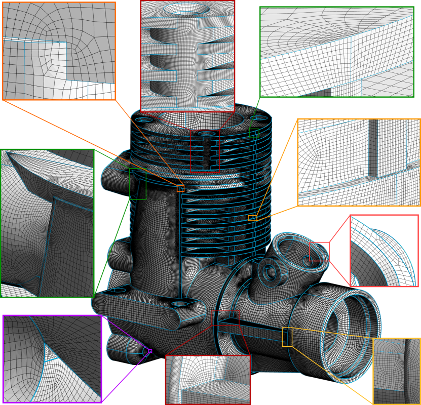
Figure 9: Quasi-structured quad mesh (261.5k vertices, 261.6k quads) of the Block model (533 faces and 1584 curves). The average SICN quality is 0.87 and the minimum is 0.11. The initial unstructured quad mesh was generated in 58 seconds and the quasi-structured improvement took 33 seconds, both with 4 CPU cores on a laptop. The number of irregular vertices was reduced from 14.4k to 3.6k.

To validate our approach and confirm its robustness, we applied it on many CAD models from existing databases (Sec. 7.1). In the next section (Sec. 7.2), we discuss the strengths and weaknesses of the approach and its positioning relative to existing techniques in the literature.

7.1 CAD databases

Test cases

We applied the end-to-end meshing pipeline to the $114$ models of the MAMBO dataset [24] and to $1000$ models the ABC dataset [23]. As the ABC dataset is huge (one million models), we randomly selected one thousand not-too-simple models for which it was possible to generate triangulations and extract a single CAD volume. This pre-selection is necessary because many models are very simple (e.g. a few CAD primitives), or are not valid, or contain lot of independent components. For all models, we applied a global sizing parameter of $0.1$ on mesh edges, i.e. edges ten times smaller than the initial very coarse CAD sampling in the triangular Delaunay mesher. In our pipeline, a size map is then produced to adapt to CAD feature locally, but the mesh resolution in the final mesh is largely controlled by this single parameter. It should be noted that using the same resolution parameter for all CAD models is very far from ideal, as the resulting meshes are either too coarse or too fine relatively to the CAD geometry, compared to what a user would choose. We still followed this procedure because it allows large scale automation and it is a good way to observe the mesher behavior in non-optimal conditions.

Results

We were able to automatically build geometrically valid quad meshes on the $114/114$ models of the MAMBO dataset and on $988/1000$ models of the ABC dataset. In the $12$ failure cases in the ABC dataset, two are topologically valid quad meshes but with tangled elements, the minimum SICN quality being respectively $-0.008$ and $-0.11$. The invalid quads are due to inverted triangles in the quad-dominant mesh, which is too coarse in some regions. The ten other failures are due to either (a) issues in the Delaunay point insertion used for the initial triangulation and frontal quad-dominant mesher or (b) performance issues (exceed the 8GB RAM or timeout after 5 hours) in the quasi-structured topological improvement when the size map is too fine. The cases (b) typically correspond to elongated models with large thin regions. Our automatic size map leads to very small elements and many millions vertices, many of them irregular, in the CAD faces. Our topological improvement strategy is not adapted in these situations because too many cavities (literally millions) are built, smoothed and remeshed, which is computationally too expensive. The above failure cases can be fixed by using a more appropriate global sizing parameter or by manually building a size map better adapted to the thin regions.

Dataset (#)	#C	#F	Q min	Q avg	#vert	% irreg. init.	% irreg.	time init. / improv.
MAMBO (114)	46	18	0.53	0.98	20.2k	1.24%	0.27 %	9.6 sec / 4.6 sec
ABC (990)	98	38	0.44	0.96	49k	2.2%	0.74 %	15.3 sec / 140.8 sec *

Table 1: Average values over all dataset models. #C and #F are the number of CAD curves and faces. Mesh statistics are computed on the final quasi-structured mesh, except for the initial percentage of irregular vertices, which is computed on the initial unstructured quad mesh. The quality metric Q is the signed inverse condition number (SICN). Time init. is the elapsed time to build the unstructured quad mesh starting from the CAD and time improv. is the elapsed time to make it quasi-structured, both computed with a single core. (*) The average run-time of 140.8 sec is high due to slow outliers (seven models took more than one hour), the median value is 5.9 seconds.

Statistics

Topological and geometrical statistics, along with figures, are available for each model in the supplementary material. Average values for some quantities are listed in Table 1. Statistically, the quads are of very high quality and the topological improvement reduces the number of irregular vertices by a factor of three (ABC) or five (MAMBO). An important proportion of the remaining irregular vertices are due to large gradients in the size map. This is caused by the global sizing parameter which is often too coarse compared to the smallest features. Global sizing parameter chosen model by model would allow a greater reduction of the number of irregular vertices, typically a factor from 5 to 10. The median and average running times for the whole pipeline are respectively 18 and 155 seconds, using a single-thread on a laptop 2.8 GHz CPU. If we normalize by the number of vertices, our complete pipeline takes around one second per thousand vertices in the output, in average.

7.2 Discussion

Statistical results (Sec. 7.1) are interesting to confirm the robustness of our approach but they are not very relevant to evaluate the mesher’s behavior. They are strongly affected by the target meshing size, i.e. smaller size would improve both regularity and quality. In the same spirit, midpoint subdivision steps would artificially improve the statistics whereas the topological structure is not changed. To better understand the mesher strengths and weaknesses, it is necessary to visually inspect the quadrilateral meshes. A detailed quad mesh of a complex model is illustrated on Fig. 9 and some of the database results are shown in the mosaic in Fig. 10.

Overview

Our end-to-end meshing pipeline is able to robustly generate quadrilateral meshes with high-quality elements on almost all CAD models, using a single global sizing parameter. There are a few failure cases, but they are due to either a very wrong target size choice or a CAD-adapted size map leading to too many vertices ($>5$M), for which we have performance issues. When using an appropriate target size, we are able to eliminate many irregular vertices (e.g. factor five to ten) in the initial unstructured mesh, while preserving a relevant global structure thanks to the cross-field singularities. In its current state, this new mesher is a viable alternative to triangular meshing in Gmsh for generic CAD models and we expect further improvements in the future. The flexibility offered by the unstructured approach makes it easy to integrate user-prescribed constraints, such as specific element sizes at given points or a custom size map given as a scalar field.

Comparison with unstructured techniques

There are two large steps in our approach: the robust generation of the initial unstructured quad mesh and its improvement via cavity remeshing. On the unstructured part, our technique is essentially an incremental improvement of standard indirect meshing [37, 38]. Thanks to the accurate cross field computation and its inherent size map (conformal scaling), we generate better vertex positions which follow integral lines of the locally integrable scaled cross field (e.g. Fig. 2.2.b). Concerning the topological improvement, we employ two topological techniques. For local and constrained configurations, we pick the best rearrangement by checking in an exhaustive list of disk quadrangulations (Sec. 6.3), which is a new technique to our knowledge. For large cavities and simple CAD faces, we use pattern-based remeshing similar to [44] but with better cavities as we are using the cross-field singularities to control their spawning and growth.

Comparison with global parametrization techniques

When the size map is dominated by the cross field scaling and not by the adaptation to small features, our approach produces meshes tending to the ones produced by global parametrization techniques (e.g. Fig. 2), except that there may be a few additional irregular vertices due to the non optimal quantization of the curves. Most global parametrization literature is from the computer graphics community and focus on smooth models without or with few feature curves, without much consideration for CAD entities. Thus, it is difficult to know if they could be adapted to strictly respect them. As they are using a global sizing parameter without adaptation to small features, the basic way to match them is to introduce strong distortions in the parametrization and it is not clear if it is possible to extract geometrically valid quads afterwards. Our approach has the advantage of working with custom size maps containing strong gradients whereas global parametrization techniques would first require to generate a cross field matching the size map, which is an open problem.

Performance

The initial unstructured quad mesh generation, starting from the CAD, is fast and is a few times the cost of triangular meshing. The computational cost of the topological improvement is less predictable as it depends on the number and size of the cavities that are candidate for remeshing. In general, the cost is similar to the initial step but it may be much higher, especially for large CAD faces with lot of vertices (¿100k). The vast majority of the time is spent doing smoothing, which is essential to guarantee geometric validity of the elements. To ensure limited running times, it is possible for the user to limit the time spent on each CAD face. In the future, we plan to develop better cavity growing strategies to deal more efficiently with large meshes by reducing the number of cavity candidates.

Thanks to the bottom-up approach, meshing and remeshing operations can be applied in parallel on each CAD face, as the boundary meshes are fixed. The scaling with the number of cores is excellent, and we are only limited by the RAM as we are using shared memory in Gmsh parallelism (OpenMP).

Figure 10: Quadrilateral meshes of models in the MAMBO [24] and ABC [24] datasets.

8 Perspectives and future work

In this work, we have presented a quadrilateral meshing pipeline which is viable for industrial use. The robustness is ensured by starting from a basic unstructured quad mesh (quad-dominant split into quads) and iteratively improving it while always checking the validity of each operation. Additional improvements stemming from recent research on cross fields are incorporated in the pipeline as guiding information, but never at the cost of robustness. Starting from this solid basis, we envision various lines of research to further enhance the topological structure of the final quad meshes.

Remaining non-essential irregular vertices

When the target size is fine and the size map is dominated by the cross field and not the CAD features, we would ideally expect to match the cross field singularities. With our approach, it requires an optimal quantization of curves, which is hardly achieved. We see two solutions to this problem, either a better initial quantization or a posteriori remeshing across CAD curves.

For the initial quantization, we should consider more the topological constraints in quadrilateral mesh. In particular, the curves of the polygonal CAD faces whose topology matches the patterns in Fig. 4 should have a number of edges such that the quantization is meshable according to the ILP problem. For the CAD faces without cross field singularities, we can assign a direction $+x,-x,+y,-y$ to each boundary curve and ensure that the sum of the edges over both axis is zero. By combining these linear constraints in a global mixed-integer problem, we should be able to produce a better initial quantization of the whole model.

A more pragmatic alternative is to eliminate the remaining irregular vertices by modifying the mesh topology globally. The remeshing cavities could grow across the CAD curves to surround opposite pairs of $+1/-1$ irregular vertices on distinct faces. The difficulty is in ensuring the CAD curves are still preserved after remeshing and in dealing with non-manifold face junctions. Another possibility is to move the pairs of $+1/-1$ in the global mesh by successively applying local mesh modifications.

Performance and large models

The main limitation of our mesher is that it is slow when dealing with large CAD face meshes ($>100k$ vertices) because there are too many remeshing cavities which are tried, and each one involves smoothing the geometry. We believe there is a lot of room for improvement in the remeshing strategy (Sec. 6.2.2), which is quite simple for the moment. A possibility could be to replace the current isotropic growth of cavities by more surgical ones which would target the non-essential irregular vertices and avoid the regions of the mesh which are already regular.

From quasi-structured to block-structured

For many applications, the best quadrilateral mesh is block-structured, meaning that its base-complex is coarse and composed of a minimum of large quadrilateral patches. This kind of meshes is interesting because it can be easily converted into a good high-order quad mesh which is ideal for accurate high-order methods. Even at low orders, the block structure allows for fast computational optimizations (e.g. implicit indexing, multigrid). Our quasi-structured meshes are not ready for such applications because their base-complexes are composed of too many patches. Even when the number of irregular vertices is low (e.g. matching the cross field singularities), the issue is that the irregular vertices are not aligned and consequently the topological chords tend to wind up over the whole model. In the future, we wish to explore ways to align the irregular vertices, such as [7], and build coarse layouts on complex CAD models. This is definitively a challenging problem as the CAD features must be fully preserved during the process.

Extension to hexahedral meshes

Hexahedral meshing is a very difficult problem, especially when trying to respect the features of CAD models. The current robust techniques are either the subdivision of a tetrahedral mesh into hexahedra or the octree-based approach [27]. Both produce meshes whose topological structure is not very good: there is a large number of irregular edges and vertices, and the hexahedra are not aligned with the model boundary. We think that exploring ways to extend the cavity remeshing technique to the 3D case could be a fruitful line of research as it would allow iterative and robust topological improvements to reduce the number of irregular edges and vertices in such meshes.

References

- Akram et al. [2021] Muhammad Naeem Akram, Lei Si, and Guoning Chen. An embedded polygon strategy for quality improvement of 2D quadrilateral meshes with boundaries. 2021.
- Bawin et al. [2020] Arthur Bawin, François Henrotte, and Jean-François Remacle. Automatic feature-preserving size field for 3D mesh generation. arXiv e-prints, pages arXiv–2009, 2020.
- Beaufort et al. [2017] Pierre-Alexandre Beaufort, Jonathan Lambrechts, François Henrotte, Christophe Geuzaine, and Jean-François Remacle. Computing cross fields a PDE approach based on the ginzburg-landau theory. Procedia Engineer., 203:219–231, 2017. ISSN 1877-7058. 10.1016/j.proeng.2017.09.799. URL https://doi.org/10.1016/j.proeng.2017.09.799.
- Ben-Chen et al. [2008] Mirela Ben-Chen, Craig Gotsman, and Guy Bunin. Conformal flattening by curvature prescription and metric scaling. In Computer Graphics Forum, volume 27, pages 449–458. Wiley Online Library, 2008.
- Blacker and Stephenson [1991] Ted D. Blacker and Michael B. Stephenson. Paving: A new approach to automated quadrilateral mesh generation. Int. J. Numer. Meth. Engng., 32(4):811–847, September 1991. ISSN 0029-5981, 1097-0207. 10.1002/nme.1620320410. URL https://doi.org/10.1002/nme.1620320410.
- Bommes et al. [2009] David Bommes, Henrik Zimmer, and Leif Kobbelt. Mixed-integer quadrangulation. ACM Trans. Graph., 28(3):1–10, July 2009. ISSN 0730-0301, 1557-7368. 10.1145/1531326.1531383. URL https://doi.org/10.1145/1531326.1531383.
- Bommes et al. [2011] David Bommes, Timm Lempfer, and Leif Kobbelt. Global structure optimization of quadrilateral meshes. In Computer Graphics Forum, volume 30, pages 375–384. Wiley Online Library, 2011.
- Bommes et al. [2013] David Bommes, Marcel Campen, Hans-Christian Ebke, Pierre Alliez, and Leif Kobbelt. Integer-grid maps for reliable quad meshing. ACM Trans. Graph., 32(4):1–12, July 2013. ISSN 0730-0301, 1557-7368. 10.1145/2461912.2462014. URL https://doi.org/10.1145/2461912.2462014.
- Borouchaki and Frey [1998] Houman Borouchaki and Pascal J. Frey. Adaptive triangular-quadrilateral mesh generation. Int. J. Numer. Meth. Engng., 41(5):915–934, March 1998. ISSN 0029-5981, 1097-0207. 10.1002/(sici)1097-0207(19980315)41:5¡915::aid-nme318¿3.0.co;2-y. URL https://doi.org/10.1002/(sici)1097-0207(19980315)41:5<915::aid-nme318>3.0.co;2-y.
- Brewer et al. [2003] Michael L Brewer, Lori Freitag Diachin, Patrick M Knupp, Thomas Leurent, and Darryl J Melander. The mesquite mesh quality improvement toolkit. In Proceedings of the international meshing roundtable. Springer, 2003.
- Bunin [2006] Guy Bunin. Non-local topological clean-up. In Proceedings of the 15th International Meshing Roundtable, pages 3–20. Springer, 2006.
- Bunin [2008] Guy Bunin. A continuum theory for unstructured mesh generation in two dimensions. Comput. Aided Geom. D., 25(1):14–40, January 2008. ISSN 0167-8396. 10.1016/j.cagd.2007.05.002. URL https://doi.org/10.1016/j.cagd.2007.05.002.
- Campen et al. [2012] Marcel Campen, David Bommes, and Leif Kobbelt. Dual loops meshing. ACM Trans. Graph., 31(4):1–11, August 2012. ISSN 0730-0301, 1557-7368. 10.1145/2185520.2185606. URL https://doi.org/10.1145/2185520.2185606.
- Campen et al. [2015] Marcel Campen, David Bommes, and Leif Kobbelt. Quantized global parametrization. ACM Trans. Graph., 34(6):1–12, November 2015. ISSN 0730-0301, 1557-7368. 10.1145/2816795.2818140. URL https://doi.org/10.1145/2816795.2818140.
- Daniels et al. [2008] Joel Daniels, Cláudio T. Silva, Jason Shepherd, and Elaine Cohen. Quadrilateral mesh simplification. In ACM SIGGRAPH Asia 2008 papers on - SIGGRAPH Asia ’08. Association for Computing Machinery, ACM Press, 2008. ISBN 9781450318310. 10.1145/1457515.1409101. URL https://doi.org/10.1145/1457515.1409101.
- Docampo-Sánchez and Haimes [2019] Julia Docampo-Sánchez and Robert Haimes. A regularization approach for automatic quad mesh generation. 28th International Meshing Roundtable, 2019.
- Ebke et al. [2013] Hans-Christian Ebke, David Bommes, Marcel Campen, and Leif Kobbelt. QEx. ACM Trans. Graph., 32(6):1–10, November 2013. ISSN 0730-0301, 1557-7368. 10.1145/2508363.2508372. URL https://doi.org/10.1145/2508363.2508372.
- Geuzaine and Remacle [2009] Christophe Geuzaine and Jean-François Remacle. Gmsh: A 3-d finite element mesh generator with built-in pre- and post-processing facilities. Int. J. Numer. Meth. Engng., 79(11):1309–1331, May 2009. ISSN 0029-5981. 10.1002/nme.2579. URL https://doi.org/10.1002/nme.2579.
- Hertzmann and Zorin [2000] Aaron Hertzmann and Denis Zorin. Illustrating smooth surfaces. In Proceedings of the 27th annual conference on Computer graphics and interactive techniques - SIGGRAPH ’00, pages 517–526. Association for Computing Machinery, ACM Press, 2000. ISBN 1581132085. 10.1145/344779.345074. URL https://doi.org/10.1145/344779.345074.
- Jakob et al. [2015] Wenzel Jakob, Marco Tarini, Daniele Panozzo, and Olga Sorkine-Hornung. Instant field-aligned meshes. ACM Trans. Graph., 34(6):1–15, November 2015. ISSN 0730-0301, 1557-7368. 10.1145/2816795.2818078. URL https://doi.org/10.1145/2816795.2818078.
- Kälberer et al. [2007] Felix Kälberer, Matthias Nieser, and Konrad Polthier. Quadcover-surface parameterization using branched coverings. In Computer graphics forum, volume 26, pages 375–384. Wiley Online Library, 2007.
- Knupp [1999] P.M. Knupp. Winslow smoothing on two-dimensional unstructured meshes. Eng. Comput-germany., 15(3):263–268, September 1999. ISSN 0177-0667, 1435-5663. 10.1007/s003660050021. URL https://doi.org/10.1007/s003660050021.
- Koch et al. [2019] Sebastian Koch, Albert Matveev, Zhongshi Jiang, Francis Williams, Alexey Artemov, Evgeny Burnaev, Marc Alexa, Denis Zorin, and Daniele Panozzo. ABC: A big CAD model dataset for geometric deep learning. In 2019 IEEE/CVF Conference on Computer Vision and Pattern Recognition (CVPR), pages 9601–9611. IEEE, IEEE, June 2019. ISBN 9781728132938. 10.1109/cvpr.2019.00983. URL https://doi.org/10.1109/cvpr.2019.00983.
- [24] Franck Ledoux. Mambo dataset. https://gitlab.com/franck.ledoux/mambo.
- Lee and Lo [1994] C.K. Lee and S.H. Lo. A new scheme for the generation of a graded quadrilateral mesh. Comput. Struct., 52(5):847–857, September 1994. ISSN 0045-7949. 10.1016/0045-7949(94)90070-1. URL https://doi.org/10.1016/0045-7949(94)90070-1.
- Marcias et al. [2015] Giorgio Marcias, Kenshi Takayama, Nico Pietroni, Daniele Panozzo, Olga Sorkine-Hornung, Enrico Puppo, and Paolo Cignoni. Data-driven interactive quadrangulation. ACM Trans. Graph., 34(4):1–10, July 2015. ISSN 0730-0301, 1557-7368. 10.1145/2766964. URL https://doi.org/10.1145/2766964.
- Maréchal [2009] Loïc Maréchal. Advances in octree-based all-hexahedral mesh generation: Handling sharp features. In Proceedings of the 18th International Meshing Roundtable, pages 65–84. Springer Berlin Heidelberg, 2009. ISBN 9783642043185, 9783642043192. 10.1007/978-3-642-04319-2_5. URL https://doi.org/10.1007/978-3-642-04319-2_5.
- McKay and Piperno [2014] Brendan D. McKay and Adolfo Piperno. Practical graph isomorphism, II. J. Symb. Comput., 60(0):94–112, January 2014. ISSN 0747-7171. 10.1016/j.jsc.2013.09.003. URL https://doi.org/10.1016/j.jsc.2013.09.003.
- Myles et al. [2014] Ashish Myles, Nico Pietroni, and Denis Zorin. Robust field-aligned global parametrization. ACM Trans. Graph., 33(4):1–14, July 2014. ISSN 0730-0301, 1557-7368. 10.1145/2601097.2601154. URL https://doi.org/10.1145/2601097.2601154.
- Owen et al. [1999] S.J. Owen, M.L. Staten, S.A. Canann, and S. Saigal. Q-morph: An indirect approach to advancing front quad meshing. Int. J. Numer. Meth. Engng., 44(9):1317–1340, March 1999. ISSN 0029-5981, 1097-0207. 10.1002/(sici)1097-0207(19990330)44:9¡1317::aid-nme532¿3.0.co;2-n. URL https://doi.org/10.1002/(sici)1097-0207(19990330)44:9<1317::aid-nme532>3.0.co;2-n.
- Palacios and Zhang [2007] Jonathan Palacios and Eugene Zhang. Rotational symmetry field design on surfaces. ACM Trans. Graph., 26(3):55, July 2007. ISSN 0730-0301, 1557-7368. 10.1145/1276377.1276446. URL https://doi.org/10.1145/1276377.1276446.
- Palmer et al. [2020] David Palmer, David Bommes, and Justin Solomon. Algebraic representations for volumetric frame fields. ACM Trans. Graph., 39(2):1–17, April 2020. ISSN 0730-0301, 1557-7368. 10.1145/3366786. URL https://doi.org/10.1145/3366786.
- Pietroni et al. [2016] Nico Pietroni, Enrico Puppo, Giorgio Marcias, Roberto Scopigno, and Paolo Cignoni. Tracing field-coherent quad layouts. In Computer Graphics Forum, volume 35, pages 485–496. Wiley Online Library, 2016.
- Ray et al. [2006] Nicolas Ray, Wan Chiu Li, Bruno Lévy, Alla Sheffer, and Pierre Alliez. Periodic global parameterization. ACM Trans. Graph., 25(4):1460–1485, October 2006. ISSN 0730-0301, 1557-7368. 10.1145/1183287.1183297. URL https://doi.org/10.1145/1183287.1183297.
- Ray et al. [2008] Nicolas Ray, Bruno Vallet, Wan Chiu Li, and Bruno Lévy. N-symmetry direction field design. ACM Trans. Graph., 27(2):1–13, April 2008. ISSN 0730-0301, 1557-7368. 10.1145/1356682.1356683. URL https://doi.org/10.1145/1356682.1356683.
- Rebay [1993] S. Rebay. Efficient unstructured mesh generation by means of Delaunay triangulation and bowyer-Watson algorithm. J. Comput. Phys., 106(1):125–138, May 1993. ISSN 0021-9991. 10.1006/jcph.1993.1097. URL https://doi.org/10.1006/jcph.1993.1097.
- Remacle et al. [2012] J.-F. Remacle, J. Lambrechts, B. Seny, E. Marchandise, A. Johnen, and C. Geuzainet. Blossom-quad: A non-uniform quadrilateral mesh generator using a minimum-cost perfect-matching algorithm. Int. J. Numer. Meth. Engng, 89(9):1102–1119, February 2012. ISSN 0029-5981. 10.1002/nme.3279. URL https://doi.org/10.1002/nme.3279.
- Remacle et al. [2013] J.-F. Remacle, F. Henrotte, T. Carrier-Baudouin, E. Béchet, E. Marchandise, C. Geuzaine, and T. Mouton. A frontal Delaunay quad mesh generator using theL norm. Int. J. Numer. Meth. Engng, 94(5):494–512, February 2013. ISSN 0029-5981. 10.1002/nme.4458. URL https://doi.org/10.1002/nme.4458.
- Sageman-Furnas et al. [2019] Andrew O. Sageman-Furnas, Albert Chern, Mirela Ben-Chen, and Amir Vaxman. Chebyshev nets from commuting PolyVector fields. ACM Trans. Graph., 38(6):1–16, November 2019. ISSN 0730-0301, 1557-7368. 10.1145/3355089.3356564. URL https://doi.org/10.1145/3355089.3356564.
- Stimpson et al. [2007] CJ Stimpson, CD Ernst, P Knupp, P Pebay, and D Thompson. The verdict geometric quality library. Sandia Lab. Report SAND2007-175, 2007.
- Takayama et al. [2014] Kenshi Takayama, Daniele Panozzo, and Olga Sorkine-Hornung. Pattern-based quadrangulation for n-sided patches. In Computer Graphics Forum, volume 33, pages 177–184. Wiley Online Library, 2014.
- Thompson et al. [1998] Joe F Thompson, Bharat K Soni, and Nigel P Weatherill. Handbook of Grid Generation. CRC Press, December 1998. ISBN 9780367802462. 10.1201/9781420050349. URL https://doi.org/10.1201/9781420050349.
- Verhetsel et al. [2019] Kilian Verhetsel, Jeanne Pellerin, and Jean-François Remacle. Finding hexahedrizations for small quadrangulations of the sphere. ACM Trans. Graph., 38(4):1–13, July 2019. ISSN 0730-0301, 1557-7368. 10.1145/3306346.3323017. URL https://doi.org/10.1145/3306346.3323017.
- Verma and Suresh [2015] Chaman Singh Verma and Krishnan Suresh. A robust combinatorial approach to reduce singularities in quadrilateral meshes. Procedia Engineer., 124:252–264, 2015. ISSN 1877-7058. 10.1016/j.proeng.2015.10.137. URL https://doi.org/10.1016/j.proeng.2015.10.137.
- Verma and Tautges [2011] Chaman Singh Verma and Tim Tautges. Jaal: Engineering a high quality all-quadrilateral mesh generator. In Proceedings of the 20th International Meshing Roundtable, pages 511–530. Springer Berlin Heidelberg, 2011. ISBN 9783642247330, 9783642247347. 10.1007/978-3-642-24734-7_28. URL https://doi.org/10.1007/978-3-642-24734-7_28.
- Viertel and Osting [2019] Ryan Viertel and Braxton Osting. An approach to quad meshing based on harmonic cross-valued maps and the ginzburg–landau theory. SIAM J. Sci. Comput., 41(1):A452–A479, January 2019. ISSN 1064-8275, 1095-7197. 10.1137/17m1142703. URL https://doi.org/10.1137/17m1142703.
- Wardetzky et al. [2007] Max Wardetzky, Miklós Bergou, David Harmon, Denis Zorin, and Eitan Grinspun. Discrete quadratic curvature energies. Comput. Aided Geom. D., 24(8-9):499–518, November 2007. ISSN 0167-8396. 10.1016/j.cagd.2007.07.006. URL https://doi.org/10.1016/j.cagd.2007.07.006.
- Winslow [1966] Alan M Winslow. Numerical solution of the quasilinear poisson equation in a nonuniform triangle mesh. J. Comput. Phys., 1(2):149–172, November 1966. ISSN 0021-9991. 10.1016/0021-9991(66)90001-5. URL https://doi.org/10.1016/0021-9991(66)90001-5.
- Yasseen et al. [2013] Z. Yasseen, A. Nasri, W. Boukaram, P. Volino, and N. Magnenat-Thalmann. Sketch-based garment design with quad meshes. Comput.-Aided Des., 45(2):562–567, February 2013. ISSN 0010-4485. 10.1016/j.cad.2012.10.041. URL https://doi.org/10.1016/j.cad.2012.10.041.