Condensation transition in the late-time position of a Run-and-Tumble particle

Abstract

We study the position distribution $P(\vec{R},N)$ of a run-and-tumble particle (RTP) in arbitrary dimension $d$, after $N$ runs. We assume that the constant speed $v>0$ of the particle during each running phase is independently drawn from a probability distribution $W(v)$ and that the direction of the particle is chosen isotropically after each tumbling. The position distribution is clearly isotropic, $P(\vec{R},N)\to P(R,N)$ where $R=|\vec{R}|$. We show that, under certain conditions on $d$ and $W(v)$ and for large $N$, a condensation transition occurs at some critical value of $R=R_{c}\sim O(N)$ located in the large deviation regime of $P(R,N)$. For $R<R_{c}$ (subcritical fluid phase), all runs are roughly of the same size in a typical trajectory. In contrast, an RTP trajectory with $R>R_{c}$ is typically dominated by a ‘condensate’, i.e., a large single run that subsumes a finite fraction of the total displacement (supercritical condensed phase). Focusing on the family of speed distributions $W(v)=\alpha(1-v/v_{0})^{\alpha-1}/v_{0}$, parametrized by $\alpha>0$, we show that, for large $N$, $P(R,N)\sim\exp\left[-N\psi_{d,\alpha}(R/N)\right]$ and we compute exactly the rate function $\psi_{d,\alpha}(z)$ for any $d$ and $\alpha$. We show that the transition manifests itself as a singularity of this rate function at $R=R_{c}$ and that its order depends continuously on $d$ and $\alpha$. We also compute the distribution of the condensate size for $R>R_{c}$. Finally, we study the model when the total duration $T$ of the RTP, instead of the total number of runs, is fixed. Our analytical predictions are confirmed by numerical simulations, performed using a constrained Markov chain Monte Carlo technique, with precision $\sim 10^{-100}$.

I Introduction

In recent years there has been a surge of interest in the study of simple stochastic models of self-propelled particles in the context of active matter, both theoretically and experimentally, for reviews see cates12 ; soft ; BDL16 ; Ramaswamy2017 ; Marchetti2018 . This class of stochastic models can describe a wide range of artificial and natural systems, e.g., vibrated granular matter WWS17 , active gels R10 ; NVG19 , bacterial motion berg_book ; cates12 ; TC08 , animal movements R10 ; VCB95 ; HBS04 ; VZ12 etc. At variance with its passive counterpart (for instance the standard Brownian motion, whose movement is driven by the random collisions with the surrounding fluid), active particles can absorb energy directly from the environment and convert it into persistent self-propelled motion. As a result, active motion violates time-reversal symmetry and these models belong to the category of out-of-equilibrium stochastic processes. In order to describe theoretically the persistence of the particle motion, one needs to introduce in the model a stochastic noise with non-vanishing time correlations. This can be done in several ways. For instance, in the active Ornstein-Uhlenbeck (AOU) model, the noise is chosen to be a Ornstein-Uhlenbeck process whose temporal correlation decays exponentially with time FNC16 ; Bonilla19 ; SRG2019 ; WKL20 . Another possibility is to include the noise in the rotational degree of freedom of the particle, as done for the active Brownian particle (ABP) model BDL16 ; seifert16 ; Franosch18 ; BMR18 ; BMR19 ; Limmer18 ; SDC20 ; MM20 ; SBS21 , where the orientation angle of the particle itself performs a Brownian motion. Finally, yet another variant is the so called run-and-tumble particle (RTP) model kac74 ; W02 ; TC08 ; cates12 , where the active particle is driven by a telegraphic noise with exponential time correlations. In this paper, we will focus on this latter version, i.e., the RTP model.

Originally known as the persistent random walk kac74 ; S87 ; Orshinger90 ; W02 ; HJ95 ; ML17 , the RTP model has been employed in recent years to describe the motion of a class of bacteria, e.g. E. coli berg_book ; cates12 ; TC08 ; CT15 ; Solon15 , which typically move alternating between phases of straight motion with constant velocity (runs) and almost instantaneous changes of direction (tumblings), as shown in Fig. 1. This model is known to exhibit complex and interesting features not just in the many-particle setting with interactions cates12 ; TC08 ; BDL16 ; CT15 ; Solon15 ; SEB16 , but even at the single-particle level MAD12 ; Angelani15 ; MJK18 ; DM18 ; EM18 ; DKM19 ; GM2019 ; SAP19 ; LMS19 ; SK19 ; MLDM20a ; MLDM20 ; DDK20 ; HMS20 ; BMRS20 ; Bressloff20 ; SBS20 ; LM20 ; PTV2020 ; DMS21 ; BMS2021 .

In the single-particle case, the RTP model can be described as follows. The particle starts initially from the origin in a $d$-dimensional continuous space. It chooses a direction isotropically and a speed $v_{1}>0$, drawn from the probability density function (PDF) $W(v)$, and starts moving in that direction ballistically with speed $v_{1}$. After a random time $\tau_{1}$, which is exponentially distributed with rate $\gamma$, the particle tumbles, i.e., it chooses a new random direction, and starts moving in the new direction with the new speed $v_{2}$, independently drawn from $W(v)$. Then, after running during an exponentially distributed time $\tau_{2}$, it tumbles again, and so on (see Fig. 1). One can either observe the trajectory for a fixed duration $T$ (fixed-$T$ ensemble) or wait until the particle undergoes exactly $N$ complete running phases (fixed-$N$ ensemble). Even if at short times these two ensembles are quite different, it is reasonable to expect that they display similar behaviors when both $T$ and $N$ are large. The RTP dynamics is thus parametrized by three quantities: (i) the tumbling rate $\gamma$ that characterizes the time scale (the motion persists in a given direction during a typical time $\gamma^{-1}$), (ii) the spatial dimension $d$ in which the RTP lives and (iii) the speed distribution $W(v)$ which is normalized to unity, i.e., $\int_{0}^{\infty}W(v)\,dv=1$. Note that in the canonical and perhaps the most well studied RTP model, the speed of the particle is a constant $v_{0}>0$ and does not vary from one run to another, corresponding to the choice $W(v)=\delta(v-v_{0})$. Nevertheless, RTP models with generic $W(v)$ have also been studied GM2019 ; MLDM20 ; MLDM20a ; BMS2021 .

One of the simplest natural questions that one can ask about a self-propelled active particle is: how does the position distribution $P(\vec{R},T)$ evolve with time $T$? Here $T$ stands either for the real time $T$ or the number of steps $N$, e.g., in the fixed-$N$ RTP model. While for the AOU model, the position distribution is trivially Gaussian at all times since the driving noise is Gaussian, for the other two models ABP and RTP, the PDF $P(\vec{R},T)$ is nontrivial. For times $T\ll T^{*}$, where $T^{*}$ is the persistence time of the driving noise (e.g., $T^{*}=\gamma^{-1}$ in RTP), the noise correlation plays a stronger role. A typical manifestation of this, for instance, in the ABP model starting from an anistropic initial condition, is that the position distribution at short times remains strongly anisotropic–a signature of activity of the process at short times BMR18 ; MM20 . However, for times $T\gg T^{*}$, the diffusion takes over and the particle behaves more like a Brownian motion at late times. As a result, the process becomes more and more isotropic as time progresses beyond $T^{*}$, i.e., $P(\vec{R},T)\to P(R,T)$, where $R=|\vec{R}|$. Moreover, due to its convergence to a Brownian motion via the central limit theorem (CLT), this position distribution $P(R,T)$ has a Gaussian shape near its peak at late times cates12 . Since the anisotropy in the position distribution is lost at late times, one can ask: is there any other remnant signature of ‘activity’ in the position distribution $P(R,T)$ at lates times $T\gg T^{*}$? It turns out that indeed one can still find signatures of activity in $P(R,T)$ at late times, but one needs to investigate the atypical large deviation tails of $P(R,T)$, thus going beyond the Gaussian shape near the peak. The non-Gaussian large deviation tails of $P(R,T)$ at late times has been computed both in the ABP model seifert16 ; BMR19 and in a class of RTP models GM2019 ; PTV2020 ; DMS21 . In both cases, the rate functions characterizing the large deviation behavior were found to carry clear signatures of activity at late times. Thus, to detect the signature of activity of the particle at late times, one needs to investigate the rare events where the particle is far away from its starting point. A relevant motivation to study such rare events is that many biological phenomena, e.g., insemination, occur when a single active particle reaches for the first time a faraway target. Let us remark in passing that another method to detect the signature of activity of a particle at late times is to confine it in an external potential– the resulting stationary state position distribution is highly non-Boltzmann and carries the signatures of activity MJK18 ; DKM19 ; TDV16 ; DD19 ; LDMS20 .

The position distribution of an RTP in the canonical model $W(v)=\delta(v-v_{0})$ was first computed in Ref. S87 in two dimensions. Later, in Ref. MAD12 , this result was extended to arbitrary dimension $d$. However, these authors did not investigate the large-deviation regime, which was first studied in detail in Ref. PTV2020 . Remarkably, it was observed that in dimensions $d>5$ and with speed distribution $W(v)=\delta(v-v_{0})$, the system undergoes a dynamical phase transition as one increases the total displacement $R$ of the particle. This turns out to be a condensation transition, in the sense that above a certain distance $R$ from the origin, the total displacement of the particle is dominated by a single very long run (see the right panel in Fig. 1). Moreover, in GM2019 , a similar condensation transition was observed for a one-dimensional RTP with a half-Gaussian speed distribution $W(v)=\sqrt{2/\pi}\,e^{-v^{2}/2}\,\theta(v)$ (where $\theta(v)$ is the Heaviside step function), when the particle is driven by a constant force. In both cases, the transition occurs in $P(R,T)$ by varying the total displacement $R$ beyond a critical value $R_{c}$ (typically of $O(T)$)–thus the total distance $R$ plays the role of a control parameter. These two examples suggest that condensation could be a general feature of the RTP model. Unfortunately, in the canonical RTP model with fixed speed $v_{0}$, this condensation occurs only in $d>5$, which is clearly not accessible physically. The motivation behind our present work is to investigate if it is possible to observe this interesting condensation transition in $P(R,T)$ in a physically accessible dimension, e.g., in $d=1,2$ or $3$. One of our main results in this paper is to show that indeed this can be achieved by appropriately choosing the speed distribution $W(v)$.

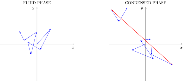
Figure 1: Left panel: Typical trajectory of a run-and-tumble particle (RTP) in two dimensions in the fluid phase. The particle starts at the origin, it chooses a direction uniformly at random and starts moving in that direction with constant speed $v_{1}$, drawn from the probability density function $W(v)$. After some random time, the particle tumbles, i.e., it changes its orientation at random and it chooses a new velocity $v_{2}$, drawn independently from $W(v)$. Then, it continues to move ballistically in this new direction, until it tumbles again, and so on. The different runs contribute to the displacement by roughly the same amount. Right panel: Typical trajectory of an RTP in the condensed phase. One single run (colored in red) dominates the trajectory.

Traditionally condensation transition is well known to occur in the momentum/energy space, e.g., the Bose-Einstein condensation in an ideal Bose gas in $d>2$ where a macroscopic number of particles condense in the single particle ground state below a critical temperature. However, condensation transition has also been observed to occur even in real space in a variety of situations–for reviews see EH05 ; M2008 . These include traffic models Krug91 ; Evans96 ; OEC98 , models of diffusion, aggregation and fragmentation MKB98 ; MKB2000 , mass transport models such as Zero Range type processes MEZ2005 ; EMZ06 ; EHM06 ; EM08 ; EMPT10 ; SEM2014 ; SEM2014b ; SEM2016 ; GB2017 , macroeconomic models BJJ2002 , network models DMS03 , discrete nonlinear Shrödinger equation RCK2000 ; GIL19 , financial models FZV13 , amongst other examples. If the parameters in these models are chosen appropriately, a condensation transition may occur upon increasing a control parameter such as the density of particles. Beyond a critical density, typically a single condensate forms in real space that contains a finite fraction of the total number of particles. For example, in the context of traffic models the analogue of the condensate is a traffic jam, while in the context of random network models, the condensate is a single node that captures macroscopic number of connections. In the RTP model studied here, the condensate is a single large run whose duration is a finite fraction of the total run time. Thus the RTP condensation provides yet another example of this phenomenon of real-space condensation.

The condensation transition that we demonstrate in the RTP model here also has implication in a broader context, namely in the classical problem in the probability theory concerning the distribution of the sum of a large number of independent and identically distributed (i.i.d.) random variables Feller_book . To establish this connection, consider the fixed-$N$ ensemble RTP model in $d$-dimensions defined above with a given tumbling rate $\gamma$ and a speed distribution $W(v)$. Since the direction after each tumbling is chosen isotropically, the position distribution $P(\vec{R},N)\equiv P(R,N)$ is clearly isotropic, i.e., it depends only on the total distance $R$ of the particle after $N$ steps, but not on its direction. Note that, for simplicity, we use the same notation for $P(R,N)$, in the fixed-$N$ ensemble, and $P(R,T)$, in the fixed-$T$ ensemble. It is then convenient to study the probability distribution $Z(X,N)$ of the total displacement $X$ in any one of the directions (say for instance the $x$-direction). Since $X$ is the $x$-component of $\vec{R}$, it is easy to show that $Z(X,N)$ and $P(R,N)$ are simply related (see Appendix A). Let $f_{d}(z)$ denote the probability distribution of the $x$-component of a random unit vector in $d$-dimensions. This can be very simply computed (see Eq. (6)). Consequently, given a random vector of fixed magnitude $R=|\vec{R}|$, its $X$ component has the distribution $(1/R)\,f_{d}(X/R)$. Finally, if $R$ itself is distributed isotropically according to $P(\vec{R},N)\equiv P(R,N)$, it follows that

$$Z(X,N)=\int_{\mathbb{R}^{d}}d\vec{R}~{}\frac{1}{R}f_{d}\left(\frac{X}{R}\right)P(R,N)\,,$$ (1)

where $d\vec{R}=S_{d}\,R^{d-1}\,dR$ with $S_{d}=2\pi^{d/2}/\Gamma(d/2)$ denoting the surface area of a $d$-dimensional unit sphere. Note that $Z(X,N)$ is a probability distribution and is normalized to unity,

$$\int_{-\infty}^{\infty}dX~{}Z(X,N)=1\,.$$ (2)

The notation $Z(X,N)$ for a probability distribution may seem a bit strange at first sight. The reason for this choice comes from the analogy to the mass-transport models (see the discussion later), where $Z(X,N)$ also plays the role of a partition function. Hence, we stick to this somewhat unfamilar notation $Z(X,N)$.

In the limit of large $N$, we expect that the position distribution will exhibit the large deviation behavior, $P(R,N)\sim\exp\left[-N\psi(R/N)\right]$ where $\psi(z)$ is the associated rate function. Then, using Eq. (1), it is easy to show that $Z(X,N)\sim\exp\left[-N\psi(X/N)\right]$, i.e., both $P(R,N)$ and $Z(X,N)$ share the same rate function $\psi(z)$ (see Appendix A). To compute the rate function $\psi(z)$ it is more convenient to consider the large deviation behavior of $Z(X,N)$ and in this paper we will follow this route. Now, denoting by $x_{i}$ the $x$-component displacement of the particle during the $i$-th run, one sees that

$$Z(X,N)=\int_{-\infty}^{\infty}dx_{1}\,\ldots\int_{-\infty}^{\infty}dx_{N}~{}\left[\prod_{i=1}^{N}p(x_{i})\right]\delta\left(X-\sum_{i=1}^{N}x_{i}\right)\,,$$ (3)

where $p(x)$ denotes the PDF of the $x$-component of a single run-vector and we have used the fact that the run-vectors are statistically independent. The delta function in Eq. (3) just enforces the total $x$-displacement after $N$ steps to be $X$. Clearly $p(x)$ is symmetric around $x=0$. The dependence on the parameters $d$, $\gamma$ and $W(v)$ is encoded in $p(x)$ (see Eq. (5)). Since $p(x)$ is normalized to unity, $Z(X,N)$ in Eq. (3) manifestly satisfies the normalization condition in Eq. (2). Thus, $Z(X,N)$ in Eq. (3) can be interpreted as the distribution of the sum of $N$ i.i.d. random variables each drawn from a symmetric $p(x)$. This classical problem is well studied in the probability literature Feller_book . In particular, it is well known that, when the second moment of $p(x)$ is finite, $Z(X,N)$ has a Gaussian shape for $|X|\sim O(\sqrt{N})$ (typical fluctuation), as a consequence of the CLT. On the other hand, when $|X|\gg N$ (atypically large fluctuation), one obtains $Z(X,N)\sim Np(X)$, corresponding to a randomly chosen variable that dominates the sum Feller_book . However, it is not completely understood how the crossover between these ‘typical’ and ‘atypical’ regimes occurs in $Z(X,N)$, as the ‘control parameter’ $X$ varies. Given a $p(x)$, is there a ‘sharp’ phase transition at some critical value $X_{c}$, or is this just a smooth crossover? While for a few specific examples of $p(x)$ this crossover between the typical and the atypical regimes have been studied nagaev , a general criterion on $p(x)$ to determine whether a sharp phase transition occurs is still missing. Our analysis of the large deviation properties of the RTP model with a general speed distribution $W(v)$ (and hence that of $p(x)$) thus sheds light on this general question as well.

In this context, let us remark that such a criterion is well established when the i.i.d. random variables are all positive, i.e., $p(x)$ has only positive support. This situation arises in a class of mass transport models defined on a lattice of $N$ sites with some prescribed rates of mass transfer between neighbouring sites EH05 ; M2008 ; MEZ2005 ; EMZ06 ; EHM06 . Here $x_{i}\geq 0$ denotes the mass at site $i$ and the dynamics conserves the total mass $X=\sum_{i=1}^{N}x_{i}$. For a large class of mass transfer rates, the system reaches at long times a stationary state where the joint distribution of masses $\{x_{i}\}$ factorise, with $p(x)$ denoting each factor that depends on the mass transfer rates EMZ2004 . Then, $Z(X,N)$ in Eq. (3) just denotes the partition function in the stationary state. In this case where $p(x)$ has only positive support ($x$ being a mass), it has been shown that the criterion for condensation depends on the tail of $p(x)$ for large $x$ EH05 ; M2008 ; MEZ2005 ; EMZ06 ; EM08 ; FZV13 . As one varies the sum $X$, the condensation occurs at some critical value $X_{c}\sim O(N)$, if and only if $e^{-c\,x}<p(x)<1/x^{2}$ as $x\to\infty$, where $c$ is any positive constant. For example, if $p(x)$ has a fat tail, $p(x)\sim x^{-\gamma}$ for large $x$ with $\gamma>2$, a condensation will occur. Similarly, if $p(x)\sim\exp[-a\,x^{\alpha}]$ for large $x$ with $a>0$ and $0<\alpha<1$ (stretched-exponential), again condensation will occur EMZ06 . However, if $p(x)\sim\exp[-a\,x^{\alpha}]$ for large $x$ with $a>0$ and $\alpha>1$, there is no condensation transition but only a smooth crossover as $X$ varies. In our problem, the variable $x_{i}$’s can be both positive and negative with $p(x)$ symmetric, and unfortunately we can not simply apply the same criterion that is valid only for positive random variables. However, by generalising the method used in Ref. EMZ06 , we show that it is possible to find a similar criterion for symmetric random variables as well.

Our main results in this paper are threefold:

1. We identify a general criterion for condensation, valid for the sum of random variables with symmetric distribution $p(x)$. In the context of the RTP model, we show that, by properly tuning the speed distribution $W(v)$, one can observe a condensation transition also in a physically accessible dimension $d\leq 3$.

2. We focus on a family of speed distributions $W(v)=(\alpha/v_{0})(1-v/v_{0})^{\alpha}\,\theta(v_{0}-v)$ supported over $v\in[0,v_{0}]$ and parametrized by $\alpha$, that allows a condensation transition according to the general criterion mentioned above. For this family of $W(v)$, we compute exactly the position distribution $Z(X,N)$ for large $N$ (see Fig. 2). In the regime where $X\sim O(N)$, we show that $Z(X,N)$ exhibits a large-deviation form $Z(X,N)\sim\exp[-N\,\psi(X/N)]$ and we compute the associated rate function $\psi(z)$. As the control parameter $X$ exceeds a critical value $X_{c}=z_{c}\,N$, we show that a condensation transition occurs. The signature of this transition is manifest in the rate function $\psi(z)$: it develops a singularity at $z=z_{c}$.

3. For any $\alpha$ and $d$, we also compute the marginal distribution $p(x|X)$ of a single-run displacement, conditioned on the total displacement $X$ (see Fig. 3). This marginal distribution $p(x|X)$ can be taken as a diagnostic of the condensation transition, as it behaves very differently in the ‘subcritical’ ($X<X_{c}$) and the ‘supercritical’ ($X>X_{c}$) phases. We show that in the supercritical phase where $X>X_{c}$, a distinct bump appears in the tail of $p(x|X)$, similar to what has been observed in mass transport models MEZ2005 ; EMZ06 .

The rest of the paper is organized as follows. In Section II we present the details of the RTP model and provide a summary of our main results. In Section III, using a grand canonical description of the system, we present a general criterion for condensation, valid for a large class of RTP models. In Section IV, we study the late-time position distribution, both in the typical and large-deviation regimes for the fixed-$N$ ensemble. We show that the phase transition manifests itself as a singularity of the rate function and we compute its order. To clarify the nature of the transition, in Section V we study the marginal probability of a single-run displacement. In Section VI, we investigate the position distribution for the fixed-$T$ ensemble. In Section VII, we present the details of the numerical simulations. Finally, in Section VIII we conclude with a summary and some open questions. Some details of the computations are presented in the appendices.

II The model and the summary of the main results

Since the paper is long, it is useful to provide a description of the model and a summary of the salient features of the main results, so that the reader is not lost in the details given in later sections. This is precisely the purpose of this section, where we also direct the reader to specific equations in later sections.

We consider a single RTP, starting from the origin and moving in $d$ dimensions. At each tumbling the speed of the particle is independently drawn from the distribution $W(v)$. As anticipated in the introduction, there are two possible set-ups: the fixed-$N$ and the fixed-$T$ ensemble. Note that if the number $N$ of running phases is fixed, then the total time $T$ can fluctuate. Alternatively, in the fixed-$T$ ensemble one fixes the total time $T$, letting $N$ fluctuate. One important difference between the two models is that in the fixed-$T$ ensemble the last running phase is yet to be completed. Therefore, the displacement of the particle during the last running phases has a different distribution with respect to the previous displacements MLDM20 ; MLDM20a . On the other hand, in the fixed-$N$ case, all displacements have the same distribution. For this reason, the analytic study of the fixed-$N$ ensemble is usually simpler. Since, as we shall see, the late-time properties of the two ensembles are very similar, we will focus on the fixed-$N$ ensemble for most of this paper. We will consider the fixed-$T$ ensemble in Section VI, where we show that the behavior of the system is qualitatively similar for the two models.

Denoting by $x_{1}\,,\ldots\,,x_{N}$ the displacements in the $x$-direction of the RTP during the $N$ running phases, we have

$$X=\sum_{i=1}^{N}x_{i}\,.$$ (4)

These increments $x_{i}$, that can be positive or negative, are i.i.d. random variables, drawn from the symmetric probability distribution MLDM20 ; MLDM20a (reproduced, for convenience, in Appendix B in this paper)

$$p(x)=\int_{0}^{\infty}dv~{}\frac{1}{v}W(v)\int_{0}^{\infty}d\ell~{}\frac{1}{\ell}f_{d}\left(\frac{x_{i}}{\ell}\right)~{}\gamma e^{-\gamma\ell/v}\,,$$ (5)

where

$$f_{d}(z)=\frac{\Gamma\left(d/2\right)}{\sqrt{\pi}\Gamma\left((d-1)/2\right)}(1-z^{2})^{(d-3)/2}\theta(1-|z|)\,,$$ (6)

$\Gamma(y)$ is the Gamma function. It is easy to check that $p(x)$ is symmetric around $x=0$. The behavior of $Z(X,N)$ depends on the dimension $d$ and the speed distribution $W(v)$ through $p(x)$ in Eq. (5). Since $p(x)$ is symmetric, $Z(X,N)$ is also symmetric, and hence it is sufficient to focus on the positive side, i.e., for $X>0$. This PDF $Z(X,N)$ can be expressed explicitly as an $N$-fold integral in terms of $p(x)$’s, as shown in Eq. (3). In this paper, we show that under specific conditions on $W(v)$ and $d$ the system undergoes a condensation phase transition at a critical value $X_{c}$ of the position $X$. For $X<X_{c}$ (subcritical phase), all the different runs $x_{1}\,,\ldots\,,x_{N}$ contribute to the total displacement by roughly the same amount. On the other hand, for $X>X_{c}$ (supercritical phase), a single run, which is referred to as the condensate, contributes to a macroscopic fraction of the displacement (see the right panel of Fig. 1). Our goal is (I) to determine the criterion on $p(x)$ for the condensation transition in $Z(X,N)$ as $X$ varies (II) when this criterion is satisfied, to determine the specific value $X_{c}$ at which the system forms a condensate, and, (III) to study, for $X>X_{c}$, the nature of this condensate, e.g., what is the distribution of run lengths carried by the condensate. The salient features of our results are highlighted below.

(I) Criterion for condensation: As in mass transport models where $p(x)$ only has positive support, we formulate a criterion for condensation in the case of symmetric $p(x)$. We show that this criterion only depends on the large-$|x|$ behavior of $p(x)$ (see Section III). By choosing the speed distribution $W(v)$ appropriately, one can find $p(x)$’s that allow for condensation. In particular, we focus on the family of speed distributions

$$W(v)=\frac{\alpha}{v_{0}}\left(1-\frac{v}{v_{0}}\right)^{\alpha-1}\,\quad{\rm where}\quad 0\leq v\leq v_{0}\,,$$ (7)

parametrized by $\alpha>0$. The constant $v_{0}>0$ represents the maximal speed that the particle can reach. Note that this family includes, as a special case, the canonical RTP model where the speed is constant from run to run. Indeed, by taking the limit $\alpha\to 0$ in Eq. (7), one finds

$$W(v)=\delta(v-v_{0}).$$ (8)

Moreover, many other relevant speed distributions belong to this class. For instance, choosing $\alpha=1$, one obtains the uniform speed distribution. Since one can always rescale space and time, without any loss of generality we set

$$v_{0}=\gamma=1$$ (9)

in the rest of the paper. Thus, our system is parametrized by the two scalars $d$ and $\alpha$. It turns out that several (but not all) properties of the condensation transition depend only on the single parameter

$$\nu=\frac{(d+2\alpha-1)}{2}\,.$$ (10)

Indeed, applying the criterion for condensation to the speed distribution in Eq. (7), we find that condensation occurs only for $\nu>2$.

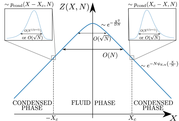
Figure 2: Schematic representation of the PDF $Z(X,N)$, for $\nu=(d+2\alpha-1)/2>2$. For $X\sim O(\sqrt{N})$ the PDF $Z(X,N)$ is Gaussian, while for $X\sim O(N)$ it assumes the large-deviation form $Z(X,N)\sim e^{-N\psi_{d,\alpha}(X/N)}$, where the rate function $\psi_{d,\alpha}(z)$ is given in Eq. (59). A dynamical phase transition occurs at $X_{c}\sim O(N)$, where $\psi_{d,\alpha}(z=X/N)$ is singular. In a small region around the critical point $X_{c}$, $Z(X,N)$ is described by the function $p_{\rm cond}(y,N)$ (see insets). For $2<\nu<3$, $p_{\rm cond}(y,N)$ has an anomalous shape, given in Eq. (16), and it varies on a scale $O(N^{1/(\nu-1)})$. For $\nu>3$, $p_{\rm cond}(y,N)$ is Gaussian with fluctuations $\sim O(\sqrt{N})$. As a consequence of the symmetry $Z(X,N)=Z(-X,N)$, an analogous transition occurs also at $-X_{c}$. For $|X|<X_{c}$ the system is in the fluid phase, while for $|X|>X_{c}$ the system is in the condensed phase.

(II) Position distribution $Z(X,N)$: Thanks to the symmetry $Z(X,N)=Z(-X,N)$, it is sufficient to focus on the case $X>0$. In the late-time limit $N\gg 1$, we consider two distinct regimes. In the typical regime $X\sim O(\sqrt{N})$, we find the central limit behavior as expected

$$Z(X,N)\simeq\frac{1}{\sqrt{4\pi DN}}e^{-X^{2}/(4DN)}\,,$$ (11)

with

$$D=\frac{2}{d(\alpha+1)(\alpha+2)}\,.$$ (12)

At this scale, no sign of activity is present. However, the signatures of the active nature of the particle can be observed in the tails of $Z(X,N)$, outside the typical Gaussian region. Indeed, in the atypical regime $X\sim O(N)$, we show that the PDF of $X$ admits the large-deviation form

$$Z(X,N)\sim\exp\left[-N~{}\psi_{d,\alpha}\left(\frac{X}{N}\right)\right]\,.$$ (13)

The rate function $\psi_{d,\alpha}(z)$ depends on both parameters $d$ and $\alpha$, and its exact expression for any $d$ and $\alpha>0$ is given in Eq. (55) for $\nu<2$, and in Eq. (59) for $\nu>2$. We will consider the scaled displacement $z=X/N$ as our control parameter. In particular, for $\nu<2$, $\psi_{d,\alpha}(z)$ is analytic for any $z>0$, while for $\nu>2$ it becomes singular at the critical point $z=z_{c}$. The critical value $z_{c}$ also depends on both parameters $d$ and $\alpha$ and is given explicitly in Eq. (60). For $z>z_{c}$, the rate function becomes exactly linear. The non-analyticity of the rate function signals the presence of a dynamical phase transition at the critical position $X_{c}=z_{c}N$. This is equivalent to the non-analyticity of the free energy in the case of equilibrium phase transitions, with the rate function playing the role of free energy. The free energy in equilibrium systems at the critical point is characterized by the order of its non-analyticity. The transition is of order $n$ if the $n$-th derivative of $\psi_{d,\alpha}(z)$ is discontinuous, while all the lower-order derivatives are continuous. In our model, we find that the order of the non-analyticity $n$ at the condensation transition is given by

$$n=\begin{cases}\left\lceil\frac{\nu-1}{\nu-2}\right\rceil\,\,\,&\text{for }2<\nu<3,\\ \\ 2\,\,\,&\text{for }\nu>3\,,\\ \end{cases}$$ (14)

where $\left\lceil y\right\rceil$ denotes the smallest integer larger than or equal to $y$. As a consequence of the $X\to-X$ symmetry of the process, an analogous transition occurs also at $-X_{c}$.

For $\nu>2$, we next zoom in the region around the critical point $z=z_{c}$ and investigate $Z(X,N)$ on a finer scale around $X=X_{c}$ (see Fig. 2). By computing $Z(X,N)$ in the vicinity of $X_{c}=z_{c}\,N$, we find that

$$Z(X,N)\simeq C_{N}~{}p_{\rm cond}\left(X_{c}-X,N\right)\,,$$ (15)

where $C_{N}$ is a positive constant and the function $p_{\rm cond}(y,N)$ depends on $N$, $\alpha$, and $d$. For $2<\nu<3$, we find that

$$p_{\rm cond}(y,N)\simeq\frac{1}{N^{1/(\nu-1)}}V_{\nu}\left(\frac{y}{N^{1/(\nu-1)}}\right)\,,$$ (16)

where the function $V_{\nu}(y)$ is given in Eq. (95) (see also Fig. (10) for a plot of this function). On the other hand, for $\nu>3$, we obtain that, for $|y|\ll\sqrt{N\log(N)}$,

$$p_{\rm cond}(y,N)\simeq\frac{1}{\sqrt{4\pi a_{d,\alpha}N}}~{}e^{-y^{2}/(4a_{d,\alpha}N)}\,,$$ (17)

where $a_{d,\alpha}$ is a positive constant given in Eq. (64). For $\nu>3$, the Gaussian shape in Eq. (17) is only valid for $|y|\ll\sqrt{N\log{N}}$. Outside this region, $p_{\rm cond}(y,N)$ has a power-law tail (see Eq. (118)). Adapting the same terminology as in mass transport models MEZ2005 ; EMZ06 , we will call the condensate ‘anomalous’ for $2<\nu<3$ and ‘normal’ for $\nu>3$. Interestingly, as we will see later, the behavior of $Z(X,N)$ close to the critical point in Eq. (15) also determines the size and the nature of the condensate that forms when $X>X_{c}$. More precisely, we show that the same function $p_{\rm cond}(y,N)$ that characterizes $Z(X,N)$ near the critical point in Eq. (15) and which is positive and normalized to one, indeed also describes the size distribution of the condensate, i.e., the probability distribution of the run length carried by the condensate (hence the subscript in $p_{\rm cond}(y)$) when the condensate forms. A schematic representation of the different regimes of $Z(X,N)$ as a function of $X$ is shown in Fig. 2.

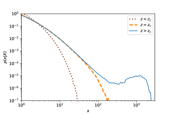
Figure 3: Numerical curves of the marginal probability $p(x|X)$ of a single-run displacement, for $\alpha=0$ and $d=8$. For $z<z_{c}$ (dotted brown line), the system is in the fluid phase and $p(x|X)$ decays exponentially fast for large $x$. At the critical point $z=z_{c}$ (orange dashed line), $p(x|X)$ develops a power-law tail. For $z>z_{c}$ (blue continuous line), the system is in the condensed phase and $p(x|X)$ still has a power-law tail and a condensate bump appears at $x=X_{\rm ex}$.

(III) Single-run marginal distribution $p(x|X)$: To understand better the nature of the dynamical phase transition described above, it is useful to study the PDF of the single-run marginal distribution $p(x|X)$, conditioned on the total displacement $X$. This is obtained by integrating the joint distribution of $\{x_{i}\}$’s over $(N-1)$ variables, while keeping fixed the sum $X=\sum_{i=1}^{N}x_{i}$ and the value of one of them, say the first one, at $x_{1}=x$. We consider only the case $\nu>2$, where the transition surely occurs. This conditional distribution $p(x|X)$ can be taken as a clear diagnostic for the condensation transition, since it behaves very differently in the subcritical ($0<z<z_{c}$) and supercritical ($z>z_{c}$) phases (see Fig. 3).

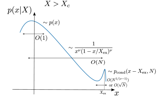
Figure 4: Qualitative behavior of the marginal probability $p(x|X)$ versus $x$ in the condensate phase. When $x\sim O(1)$, we find that $p(x|X)\sim p(x)$, where $p(x)$ is the distribution of a single displacement, given in Eq. (5). For $1\ll x\ll N$, we find that $p(x|X)\sim(x(1-x/X_{\rm ex}))^{-\nu}$, where $X_{\rm ex}=X-X_{c}$ and $\nu=(d+2\alpha-1)/2$. At $x\simeq X_{\rm ex}\sim O(N)$, a condensate bump appears in the tail of $p(x|X)$. The shape $p_{\rm cond}(y,N)$ of the bump depends continuously on $\nu$. For $2<\nu<3$, the condensate bump has an anomalous shape, with fluctuations of order $N^{1/(\nu-1)}$ (see Eq. (16)). For $\nu>3$, the bump has a Gaussian shape with fluctuations of order $\sqrt{N}$.

Subcritical phase ($0<z<z_{c}$): In this case, we show that $p(x|X)$ decreases monotonically with increasing $x$ and for $x\gg 1$

$$p(x|X)\sim\frac{1}{x^{\nu}}e^{-x/\xi}\,,$$ (18)

where $\xi>0$ depends on $z=X/N$. Thus, below the transition $z<z_{c}$, the marginal distribution $p(x|X)$ decays exponentially fast over a scale $\xi$. For this reason, all the displacements $x_{1}\,,\ldots x_{N}$ contribute “democratically” to the total displacement $X$ and thus this subcritical regime behaves like a fluid. Notably, when $z\to z_{c}$ from below the typical length $\xi$ diverges.

Critical phase ($z=z_{c}$): Exactly at the critical point $z=z_{c}$, the conditional distribution still decays monotonically with increasing $x$, but develops a power-law tail for large $x$

$$p(x|X)\sim\frac{1}{x^{\nu}}\,,$$ (19)

where we recall $\nu=(d+2\alpha-1)/2$.

Supercritical phase ($z>z_{c}$): For $z>z_{c}$, the distribution $p(x|X)$ becomes a non-monotonic function of $x$ (see Fig. 3). When $x\sim O(1)$, we show that $p(x|X)\sim p(x)$, i.e, the conditioned distribution is insensitive to the constraint, and behaves like a constraint-free system. For $x\gg 1$, the function decays with increasing $x$ as a power law, as at the critical point in Eq. (19). However, this power law behavior ceases to hold when $x$ approaches $X_{\rm ex}=X-z_{c}N>0$ (analogously to the excess mass $M_{\rm ex}$ in the mass transport models MEZ2005 ; EMZ06 ). For $1\ll x\ll X_{\rm ex}$ we get

$$p(x|X)\simeq\frac{A_{d,\alpha}}{x^{\nu}}\frac{1}{(1-x/X_{\rm ex})^{\nu}}\,,$$ (20)

where $A_{d,\alpha}>0$ is given in Eq. (33). This describes the shoulder region before the bump in Fig. 3 in the supercritical phase. The approximate expression in Eq. (20) breaks down when $x\to X_{\rm ex}$. Indeed, at $x\sim X_{\rm ex}$, a bump appears in the tail of $p(x|X)$, where

$$p(x|X)=\frac{1}{N}p_{\rm cond}(x-X_{\rm ex},N)\,.$$ (21)

Thus, the function $p_{\rm cond}(x-X_{\rm ex},N)$ describes the shape of the condensate. The bump is centered at $X_{\rm ex}$ and its width vanishes relative to its location for large $N$ (see Fig. (4)). The area under this bump is the probability that a condensate appears in a particular single-run displacement. We find that

$$\int_{-\infty}^{\infty}dy~{}\frac{1}{N}\,p_{\rm cond}(y,N)=\frac{1}{N}\,,$$ (22)

meaning that only one condensate appears in the system. We recall that, for $2<\nu<3$, $p_{\rm cond}(y,N)$ is given in Eq. (16) and the condensate has anomalous fluctuations of order $N^{1/(\nu-1)}$, where $1/2<1/(\nu-1)<1$. For this reason, we denote the phase $2<\nu<3$ as the anomalous condensate phase. On the other hand, for $\nu>3$, $p_{\rm cond}(y,N)$ is given in Eq. (17) and the bump has a normal shape around its peak, with fluctuations of order $\sqrt{N}$. Hence, we call this region the normal condensate phase. Note however that the Gaussian shape is valid only for $|y|\ll\sqrt{N\log{N}}$ and that outside this region, the bump has a power-law tail.

Finally, for $x\gg X_{\rm ex}$ and for any $\nu>2$, we observe that $p(x|X)$ gets cut-off around $X\sim O(N)$ (finite-size effect) and this cut-off behavior can be described by a large deviation form

$$p(x|X)\sim\exp\left[-N\chi\left(\frac{x}{N},\frac{X}{N}\right)\right]\,,$$ (23)

where the rate function $\chi(y,z)>0$ is given in Eq. (131). Thus, configurations where a single-run displacement is larger than $X_{\rm ex}$ become exponentially rare for large $N$.

The qualitative behavior of $p(x|X)$ in the three phases (subcritical, critical and supercritical) is shown in Fig. 3. In Fig. 4, we focus on the condensed phase $X>X_{c}$ and we present a schematic representation of the different regimes of $p(x|X)$ as a function of $x$.

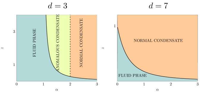
Figure 5: Left panel. Phase diagram in the $(\alpha,z)$ plane, for $d=3$. For $\alpha<1$ the system is always in the fluid phase, where all runs contribute by roughly the same amount to the total displacement of the particle. For $\alpha>1$, the system undergoes a dynamical condensation transition at a critical value $z_{c}$ of the control parameter $z$ (continuous black line). The exact expression of $z_{c}$ is given in Eq. (60). For $z<z_{c}$, the system is in the fluid phase, while above the transition the system is in the condensate phase. In particular, for $1<\alpha<2$, the system is in the anomalous condensate phase, while for $\alpha>2$ the system is in the normal condensate phase. Right panel. Phase diagram in the $(\alpha,z)$ plane, for $d=7$. For $z<z_{c}$, the system is in the fluid phase, while for $z>z_{c}$ it is in the normal condensate phase. For $d\geq 7$, the system is never in the anomalous condensed phase.

To sum up, we find that

• for $\nu<2$, the system is always in the fluid phase;

• for $2<\nu<3$, the system is in the anomalous condensate phase for $X>X_{c}$ and the order of the transition depends continuously on $\nu$;

• for $\nu>3$, the system is in the normal condensate phase for $X>X_{c}$ and the transition is of second order.

For the RTP model, we thus also find the two different types of condensed phases ‘anomalous’ and ‘normal’, as in the case of mass transport models MEZ2005 ; EMZ06 . The behavior of the system is determined by three parameters: the two system parameters $(\alpha,d)$ and the control parameter $z=X/N$. This would correspond to a three-dimensional phase diagram, which is of course complicated to display. For this reason, we present two different slices of the phase diagram. In the left panel of Fig. 5, we focus on the physical dimension $d=3$ and we show the $(\alpha,z)$ phase space. In three dimensions and for $\alpha<1$, condensation can not occur. Conversely, for $\alpha>1$, above some critical value $z_{c}$ of the parameter $z$ (given in Eq. (60)), the system undergoes a condensation transition. In particular, for $1<\alpha<2$ and $z>z_{c}$, the condensate is anomalous. In contrast, for $\alpha>2$ and $z>z_{c}$, the condensate is normal. Increasing the dimension $d$, the region of the phase space corresponding to the anomalous condensate phase shrinks, until, at $d=7$, it disappears. Indeed, for $d\geq 7$, the system can either be in the fluid ($z<z_{c}$) or in the normal condensate phase ($z>z_{c}$). In the right panel of Fig. 5, we present the $(z,\alpha)$ phase diagram for $d=7$ which shows that only two phases ‘fluid’ and ‘normal condensate’ can occur.

III Grand canonical criterion for condensation

In this section, we provide a general argument that allows us to determine the conditions that are necessary for condensation. This approach is based on a grand canonical description of the system and will also allow us to determine the critical value $X_{c}$ of the total displacement $X$ at which the phase transition occurs. Note however that the method presented below does not give any information about the nature of the condensed phase, which will be analyzed in detail in the next sections.

In order to investigate the condensation transition, we will focus on the large-deviation regime where $X$ scales linearly with the number $N$ of runs, in the limit $N\to\infty$. We define the scaled distance $z=X/N$, which will be the control parameter of our system. To establish when condensation occurs, we adopt a grand canonical description, as was done for positive-only i.i.d. random variables in the context of mass models MEZ2005 ; EMZ06 . There will be important differences however from the mass models. In the grand canonical approach we assume that the variables $x_{i}$ in Eq. (3) become decoupled from each other. To do this, we remove the hard delta-function constraint in Eq. (3) and replace it by a factor $e^{-\mu\,\sum_{i=1}^{N}x_{i}}$ where $\mu$ plays the role of the negative chemical potential or equivalently a Lagrange multiplier. We fix the value of $\mu$ by fixing the average $\langle X\rangle$. In other words, we let the total displacement $X$ free to fluctuate in the grand canonical description, but with its average $\langle X\rangle$ kept fixed. Provided this approach works, the canonical partition function given by the $N$-fold integral in Eq. (3) is replaced by the grand-canonical partition function defined as

$$Z_{\rm GC}(\mu,N)=\int_{-\infty}^{\infty}\prod_{i=1}^{N}p(x_{i})\,e^{-\mu\,x_{i}}\,dx_{i}=\left[\int_{-\infty}^{\infty}p(x)\,e^{-\mu x}\,dx\right]^{N}\,,$$ (24)

with $p(x)$ given in Eq. (5). Thus, in the grand canonical ensemble, the $N$ runs are completely independent, each drawn from the normalized PDF

$$p_{\mu}(x)=\frac{e^{-\mu x}\,p(x)}{\int_{-\infty}^{\infty}dx\,e^{-\mu x}\,p(x)}\,.$$ (25)

We recall that the PDF $p(x)$ is symmetric around $x=0$. The parameter $\mu$ can be determined from the following condition on the average displacement

$$\langle X\rangle=\sum_{i=1}^{N}\langle x_{i}\rangle=z\,N\,,$$ (26)

where the average is with respect to the distribution $p_{\mu}(x)$ in Eq. (25). This gives

$$z=f(\mu)\equiv\frac{\int_{-\infty}^{\infty}dx\,x~{}e^{-\mu x}p(x)}{\int_{-\infty}^{\infty}dx~{}e^{-\mu x}p(x)}\,.$$ (27)

The main idea behind the condensation criterion that we are going to present is that, when Eq. (27) admits a solution, the canonical and grand canonical descriptions are equivalent and we will call the system to be in the ‘fluid’ phase. On the other hand, if for some value of $z$, Eq. (27) ceases to have a solution for $\mu$, then the two ensembles are not no longer equivalent, signalling a possible phase transition. To proceed, it is useful to define the limiting value

$$c=-\lim_{x\to\infty}\frac{\log(p(x))}{x}\,.$$ (28)

We distinguish different cases, depending on $c$.

The case $c=\infty$: First, we consider the case $c=\infty$, corresponding to a PDF $p(x)$ that decays faster than any exponential for large $|x|$. Let us first examine the two integrals, respetively in the numerator and the denominator of Eq. (27). When $p(x)$ decays faster than any exponential, clearly both integrals in Eq. (27) exist for any $\mu$, i.e., for all $-\infty<\mu<\infty$. Then the function $f(\mu)$ in Eq. (27) is a monotonically decreasing function of $\mu$ in the range $\mu\in[-\infty,\infty]$, going from $\infty$ (as $\mu\to-\infty$) to $-\infty$ (as $\mu\to\infty$). Then, for any value of $z$, there is a unique solution of the equation (27) for $\mu$. This means that the canonical and grand canonical descriptions are equivalent, the system remains a fluid for all $z$, and never develops a condensate.

The case $0<c<\infty$: This corresponds to a distribution $p(x)$ that decays exponentially fast as $p(x)\sim e^{-c|x|}$ for large $|x|$. Then, the parameter $\mu$ can only take values only in the interval $(-c,c)$ in order that both integrals in Eq. (27) converge. It is useful to define the auxiliary function

$$\tilde{p}(x)=p(x)e^{c|x|}\,.$$ (29)

The function $f(\mu)$ in Eq. (27) is again a decreasing odd function of $\mu$, but now only in the bounded range $\mu\in[-c,c]$. It is then easy to see from Eq. (27) that if $\tilde{p}(x)$ decays slower than $1/|x|^{2}$ for large $|x|$, then $f(\mu)$ diverges at the two edges: $f(\mu)\to+\infty$ as $\mu\to-c$ and $f(\mu)\to-\infty$ as $\mu\to c$ (see Fig. 6). Hence, for a given $z$, one can always find a solution to the equation $f(\mu)=z$ in Eq. (27). Consequently, there is no transition.

On the other hand, if $\tilde{p}(x)$ decays faster than $1/|x|^{2}$ then the integrals in Eq. (27) are convergent for all $\mu\in[-c,c]$. In particular, at the left edge, the function $f(\mu)$ approaches

$$z_{c}=f(-c)=\frac{\int_{-\infty}^{\infty}dx\,x~{}e^{cx}p(x)}{\int_{-\infty}^{\infty}dx~{}e^{cx}p(x)}<\infty\,.$$ (30)

Thus, for $z<f(-c)$, a solution of Eq. (27) always exists. On the other hand, for $z>f(-c)$, there is no solution to Eq. (27), signalling a condensation transition. Thus, the phase transition occurs at the critical value $z_{c}=f(-c)$. Using the symmetry, a similar condensation will also occur for $z<-z_{c}=f(c)$. Note however that this grand canonical description does not shed light on the precise nature of the condensed phase. Indeed, to understand the behavior of the system above the transition, a detailed analysis of the canonical PDF in Eq. (3) is required as in the case of mass transport models EMZ06 .

The case $c=0$: In this case, $p(x)$ decays slower than an exponential as $|x|\to\infty$. Thus, the integrals in the denominator and numerator of Eq. (27) exist for $\mu=0$. For any nonzero $\mu$, the integrals diverge, either as $x\to-\infty$ (if $\mu>0$), or as $x\to\infty$ (if $\mu<0$). Thus, the grand canonical description fails completely here. However, we believe that the system still undergoes a condensation transition if $p(x)$ decays, for large $|x|$ faster than $1/|x|^{3}$. The reason behind this conjecture is the following. If $p(x)$ decays faster than $1/|x|^{3}$, then its second moment is finite and the CLT applies. Therefore, for $X\sim\sqrt{N}$, $Z(X,N)$ assumes a Gaussian shape. On the other hand, for $X\sim N$, we expect

$$Z(X,N)\sim Np(X)\,,$$ (31)

where the right-hand side corresponds to a configuration where one of the runs absorbs the whole displacement $X$. Thus, $Z(X,N)$ is described by two regimes: the typical Gaussian regime for $X\sim\sqrt{N}$ and the fat-tailed regime for $X\sim N$. In this case, for $X\sim O(N)$, the distribution $Z(X,N)$ does not have a large deviation behavior of the type, $Z(X,N)\sim\exp[-N\,\psi(X/N)]$, and thus condensation can not happen on a scale $X\sim O(N)$. However, if the central CLT region has to match the tail behvaior in Eq. (31), we believe that a condensation should occur at a shorter scale $X\sim N^{\gamma}$, where $1/2<\gamma<1$. This has already been hinted in Ref. GM2019 which studied a particular example, though there $p(x)$ was asymmetric.

In the complementary case when $p(x)$ decays slower than $1/|x|^{3}$, the CLT does not hold and, already in the typical regime, $X$ is dominated by the maximum of $x_{1}\,,\ldots x_{N}$ BG90 . Thus, in this case, condensation spontaneously occurs at any scale and no dynamical phase transition takes place.

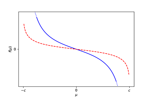
Figure 6: The function $f(\mu)$ versus $\mu$. If $f(\mu)$ diverges when $\mu\to-c$ (continuous blue curve), Eq. (27) will admit a solution for $\mu$ and no transition occurs. If $f(\mu)$ goes to a finite value $f(-c)$ when $\mu\to-c$ (dashed red curve), Eq. (27) will always admit a solution only for $z<f(-c)$ and at $z=f(-c)$ a condensation transition occurs.

In the rest of this section, we will show that one can obtain several RTP models that satisfy the condensation criterion. This can be achieved by properly tuning the speed distribution $W(v)$. Below, we provide few examples of $W(v)$ that lead to condensation.

• $W(v)=\alpha(1-v)^{\alpha-1}$ with $0<v<1$, as mentioned in Eq. (7) with $v_{0}=1$. In this case, for arbitrary $d$, one can show that for large $|x|$ (see Appendix C)

  $$p(x)\simeq A_{d,\alpha}e^{-|x|}\frac{1}{|x|^{\nu}}~{}\,,$$ (32)

  where

  $$A_{d,\alpha}=\frac{\Gamma\left(d/2\right)\alpha\Gamma\left(\alpha\right)}{\sqrt{\pi}}2^{(d-3)/2}\,\quad{\rm and}\quad\nu=\frac{(d+2\alpha-1)}{2}\,.$$ (33)

  In this case $c=1$ from Eq. (28) and, applying the criterion described above, we find that the transition is possible only for $\nu>2$, i.e., for $d+2\alpha>5$. Recalling that the limit $\alpha\to 0$ corresponds to the canonical RTP model with fixed velocity (i.e., $W(v)=\delta(v-1)$), we recovered that for the fixed-velocity RTP model condensation is possible only for $d>5$. This was first observed in PTV2020 . Plugging the expression for $p(x)$, given in Eq. (5), into Eq. (30), we obtain the critical value $z_{c}$ explicitly, valid for arbitrary $d$ and $\alpha$,

  $$z_{c}=\frac{4}{d(1+\alpha)(2+\alpha)}\frac{{}_{4}F_{3}\left[3/2,~{}3/2,~{}2,~{}2;(2+d)/2,~{}(3+\alpha)/2,~{}(4+\alpha)/2;1\right]}{{}_{4}F_{3}\left[1/2,~{}1/2,~{}1,~{}1;d/2,~{}(1+\alpha)/2,~{}(2+\alpha)/2;1\right]}\,,$$ (34)

  where ${}_{4}F_{3}$ is the standard hypergeometric function defined more precisely in Eq. (41). In the next sections, we will focus on this family of speed distributions, parametrized by $\alpha$.

• $W(v)=\sqrt{\frac{2}{\pi}}\,e^{-v^{2}/2}$ with $v>0$. Considering $d=1$ and using Eq. (5), one can show that, for $|x|\gg 1$,

  $$p(x)\sim{|x|}^{-1/3}e^{-3|x|^{2/3}/2}\,.$$ (35)

  In this case $p(x)$ decays slower than any exponential, thus $c=0$. Moreover, $p(x)$ decays faster than $1/|x|^{3}$ and thus according to our conjecture, a condensation transition should occur. The condensation transition in the RTP model with this particular half-Gaussian speed distribution was studied in Ref. GM2019 , but in the presence of an additional constant force.

• $W(v)\sim 1/v^{\beta}$ for large $v$ with $\beta>1$. In this example, for $d=1$, it is easy to show from Eq. (5) that $p(x)\sim 1/|x|^{\beta}$ for large $|x|$. Thus, we find $c=0$ and one has condensation only if $\beta>3$, according to our conjecure.

Let us recall that in the case of the sum of positive-only i.i.d. random variables, a similar condensation criterion was established EMZ06 . In that case, one can still define the limiting value $c$ in Eq. (28). Then, if $c=\infty$, no condensation happens. For $0\leq c<\infty$, condensation happens only if $\tilde{p}(x)=e^{cx}p(x)$ decays faster than $1/x^{2}$.

IV Position distribution

In this section, we want to investigate the PDF $Z(X,N)$ of the total $x$-component displacement $X$, where $X=\sum_{i=1}^{N}x_{i}$, by analysing fully the $N$-fold integral in Eq. (3), thus going beyond the grand canonical description discussed in the previous section. We will first derive an exact expression for $Z(X,N)$, valid for any $X$ and $N$. Then, focusing on large $N$, we study both the typical regime $X\sim O(\sqrt{N})$, where $Z(X,N)$ is Gaussian, and the large-deviation regime $X\sim O(N)$, where $Z(X,N)$ assumes a large deviation form, $Z(X,N)\sim\exp\left[-N\psi_{d,\alpha}(X/N)\right]$, with a rate function $\psi_{d,\alpha}(z)$ that we compute exactly. Under specific conditions on $d$ and $\alpha$, we show that $\psi_{d,\alpha}(z)$ becomes singular at a critical value $z_{c}$ of the scaled displacement $z=X/N$. This singularity corresponds to a condensation phase transition.

We recall that the PDF $Z(X,N)$ can be written as (see Eq. (3))

$$Z(X,N)=\int_{-\infty}^{\infty}dx_{1}\,\ldots\int_{-\infty}^{\infty}dx_{N}\,\prod_{i=1}^{N}p(x_{i})~{}\delta\left(X-\sum_{i=1}^{N}x_{i}\right)\,,$$ (36)

where the delta function constraints the final position to be $X$ and $p(x)$ is given in Eq. (5), with $W(v)=\alpha(1-v)^{\alpha-1}$ for $0\leq v\leq 1$ and $W(v)=0$ otherwise. To proceed, we recall the integral representation of the delta function

$$\delta(X)=\frac{1}{2\pi i}\int_{\Gamma}dq~{}e^{-qX}\,,$$ (37)

where the integral is performed over the imaginary-axis Bromwich contour $\Gamma$ in the complex $q$ plane. Plugging this integral expression into Eq. (36), we find

$$Z(X,N)=\frac{1}{2\pi i}\int_{\Gamma}dq~{}e^{qX}\left[\hat{p}(q)\right]^{N}\,,$$ (38)

where

$$\hat{p}(q)=\int_{-\infty}^{\infty}dx~{}e^{-qx}p(x)\,.$$ (39)

Substituting $W(v)=\alpha\,(1-v)^{\alpha-1}$ over $v\in[0,1]$ in Eq. (5), we first evaluate $p(x)$ and then compute $\hat{p}(q)$ using Eq. (39). Using Mathematica, we get

$$\hat{p}(q)={}_{4}F_{3}\left(\frac{1}{2},\frac{1}{2},1,1;\frac{d}{2},\frac{1+\alpha}{2},\frac{2+\alpha}{2};q^{2}\right)\,,$$ (40)

where ${}_{p}F_{q}(\alpha_{1}\,,\ldots\alpha_{p};\beta_{1}\ldots\beta_{q};q)$ denotes the generalized hypergeometric function, defined as

$${}_{p}F_{q}(\alpha_{1}\,,\ldots\alpha_{p};\beta_{1}\ldots\beta_{q};z)=\sum_{n=0}^{\infty}\frac{(\alpha_{1})_{n}\ldots(\alpha_{p})_{n}}{(\beta_{1})_{n}\ldots(\beta_{q})_{n}}\frac{z^{n}}{n!}\,,$$ (41)

where $(a)_{n}$ is the rising factorial (or Pochhammer symbol), defined as

$$(a)_{n}=\begin{cases}1~{}~{}~{}&\text{ if }\,\,n=0\\ \\ a(a+1)(a+2)\ldots(a+n-1)~{}~{}~{}&\text{ if }\,\,n\geq 1~{}.\\ \end{cases}$$ (42)

Thus, we find

$$Z(X,N)=\frac{1}{2\pi i}\int_{\Gamma}dq~{}\exp\left[qX+NS_{d,\alpha}(q)\right]\,,$$ (43)

where

$$S_{d,\alpha}(q)=\log\left[{}_{4}F_{3}\left(\frac{1}{2},\frac{1}{2},1,1;\frac{d}{2},\frac{1+\alpha}{2},\frac{2+\alpha}{2};q^{2}\right)\right]\,.$$ (44)

Note that this result is exact for any $X$ and $N$. We are now interested in extracting the behavior of $Z(X,N)$ in the limit of large $N$.

IV.1 Typical regime

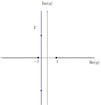
Figure 7: Analytic structure of the function $S_{d,\alpha}(q)$, given in Eq. (44). For any $d$ and $\alpha$, $S_{d,\alpha}(q)$ has two branch cuts (the grey wiggly lines in figure) in the real-$q$ axis, for $q<-1$ and for $q>1$. The continuous blue line represents the Bromwich contour $\Gamma$, defined in the text.

First, we investigate the typical regime where $X\sim\sqrt{N}$. Substituting $X=\sqrt{N}\,y$ in Eq. (43), where the variable $y$ is assumed to be of order one, we obtain

$$Z(X=\sqrt{N}\,y,N)=\frac{1}{2\pi i}\int_{\Gamma}dq~{}\exp\left[q\sqrt{N}\,y+N\,S_{d,\alpha}(q)\right]\,.$$ (45)

We now perform the change of variable $q\to q\sqrt{N}$ and we obtain

$$Z(X=\sqrt{N}y,N)=\frac{1}{2\pi i\sqrt{N}}\int_{\Gamma}dq~{}\exp\left[q~{}y+NS_{d,\alpha}\left(\frac{q}{\sqrt{N}}\right)\right]\,.$$ (46)

We expand the right-hand side of Eq. (46) for large $N$, using Eq. (44) and the small-argument expansion of the generalized hypergeometric function Gradshteyn_book , and we find

$$Z(X=\sqrt{N}y,N)\simeq\frac{1}{2\pi i\sqrt{N}}\int_{\Gamma}dq~{}\exp\left(q~{}y+\frac{2q^{2}}{d(\alpha+1)(\alpha+2)}\right)\,.$$ (47)

Finally, performing the Gaussian integral over $q$ we obtain the results announced in Eqs. (11) and (12). Thus, in this regime, the distribution of the final position of the particle is Gaussian. This is a consequence of the CLT, since $X$ is the sum of $N$ i.i.d. random variables with finite variance. This is consistent with the fact that, for any $N$, the variance of $X$ is simply given by

$$\langle X^{2}\rangle=N\int_{-\infty}^{\infty}dx~{}x^{2}~{}p(x)=\frac{4N}{d(\alpha+1)(\alpha+2)}\,.$$ (48)

The result in Eq. (11) tells us that, for late times, the RTP has typically a diffusive behavior, similar to the one of a passive Brownian motion. In other words, at the scale $X\sim\sqrt{N}$ the position distribution of the RTP does not show any signs of activity. In order to observe the signatures of the active nature of the particle, it is necessary to investigate the large-deviation regime, where $X\sim N$. It is possible to show that the result in Eq. (11) is valid on a larger region than the one predicted by the CLT, for any $|X|\ll N^{3/4}$ (see Appendix D).

IV.2 Large-deviation regime

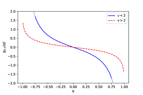
Figure 8: The function $g_{d,\alpha}(q)$ versus $q$ for different values of $\nu=(d+2\alpha-1)/2$. For any $\nu$, $g_{d,\alpha}(q)$ is a decreasing odd function of $q$. For $\nu<2$, $g_{d,\alpha}(q)$ diverges when $q\to-1$, while for $\nu>2$ it goes to the finite value $g_{d,\alpha}(-1)$.

To proceed, we define the rescaled variable $z=X/N$. From Eq. (43), we obtain

$$Z(X=Nz,N)=\frac{1}{2\pi i}\int_{\Gamma}dq~{}e^{N\left[qz+S_{d,\alpha}(q)\right]}\,.$$ (49)

where $S_{d,\alpha}(q)$ is given in Eq. (44). We recall that the integral in Eq. (49) is performed over the imaginary-axis Bromwich contour $\Gamma$ in the complex-$q$ plane. For any $d$ and $\alpha$, the complex function $S_{d,\alpha}(q)$ has two branch cuts running in the real-$q$ axis for $q<-1$ and $q>1$ (see Fig. 7).

We first try to compute the integral in Eq. (49) by saddle-point approximation. Assuming a saddle-point exists, it must satisfy $\frac{d}{dq}[qz+S_{d,\alpha}(q)]=0$. This gives the saddle-point equation

$$z=g_{d,\alpha}(q)\equiv-S^{\prime}_{d,\alpha}(q)\,.$$ (50)

Using the expression of $S_{d,\alpha}(q)$ in Eq. (44), we find

$$g_{d,\alpha}(q)=-\frac{4q}{d(\alpha+1)(\alpha+2)}\frac{{}_{4}F_{3}\left(\frac{3}{2},\frac{3}{2},2,2;\frac{2+d}{2},\frac{3+\alpha}{2},\frac{4+\alpha}{2};q^{2}\right)}{{}_{4}F_{3}\left(\frac{1}{2},\frac{1}{2},1,1;\frac{d}{2},\frac{1+\alpha}{2},\frac{2+\alpha}{2};q^{2}\right)}\,.$$ (51)

Note that, identifying $\mu=q$, the saddle point equation (50) is the same condition as the one that fixes the chemical potential $\mu$ in Eq. (27) in the grand canonical argument for condensation. One can check that, since $z$ is real, the solution $q^{*}(z)$ of the saddle-point equation in (50) has to be real. Moreover, due to the branch cuts of the function $S_{d,\alpha}(q)$ (see Fig. 7), $q^{*}(z)$ has to belong to the real interval $(-1,1)$. Therefore, it is instructive to analyze the behavior of $g_{d,\alpha}(q)$ for $q\in(-1,1)$. First of all, for any $d$ and $\alpha$, it is easy to show that $g_{d,\alpha}(q)$ is a decreasing odd function of $q$ along the real interval $q\in[-1,1]$, such that $g_{d,\alpha}(q)>0$ for $q<0$ and $g_{d,\alpha}(q)<0$ for $q>0$ (see Fig. 8). To proceed, we need the following asymptotic expansion for the generalized hypergeometric function, valid for $q\to 1$ from below buhring

$${}_{4}F_{3}\left(\alpha_{1},~{}\alpha_{2},~{}\alpha_{3},~{}\alpha_{4};\beta_{1},~{}\beta_{2},~{}\beta_{3};q\right)=\sum_{n=0}^{\infty}a_{n}(1-q)^{n}+(1-q)^{\varphi}\,\sum_{n=0}^{\infty}b_{n}(1-q)^{n}\,,$$ (52)

where $a_{n}$ and $b_{n}$ are constants that depend on the parameters of the function (for the precise expressions of $a_{n}$ and $b_{n}$ see buhring ) and

$$\varphi=\sum_{j=1}^{3}\beta_{j}-\sum_{j=1}^{4}\alpha_{j}\,.$$ (53)

Note that the formula in Eq. (52) is only valid if $\varphi$ is not an integer. In the case of integer $\varphi$, logarithmic corrections are present in the asymptotic expansion in Eq. (52) buhring . Using Eq. (52), it is easy to show that, for $\nu<2$ (where we recall that $\nu=(d+2\alpha-1)/2$), $g_{d,\alpha}(q)$ diverges when $q\to-1$. Thus, for $\nu<2$ the saddle-point equation (50) admits a unique solution for any $z$ and we obtain

$$Z(X,N)\simeq\frac{1}{\sqrt{2\pi|S^{\prime\prime}_{d,\alpha}\left[q^{*}(X/N)\right]|N}}\exp\left[-N\psi_{d,\alpha}\left(\frac{X}{N}\right)\right]\,,$$ (54)

where

$$\psi_{d,\alpha}(z)=-z~{}q^{*}(z)-S_{d,\alpha}(q^{*}(z))\,,$$ (55)

$q^{*}(z)$ is the unique solution of Eq. (50) and $S^{\prime\prime}_{d,\alpha}(q)$ is the second derivative of $S_{d,\alpha}(q)$ with respect to $q$. For special values of $d$ and $\alpha$, it is possible to find an explicit expression for $\psi_{d,\alpha}(z)$. For instance, in the special case $d=2$ and $\alpha=0$, we find

$$\psi_{2,0}(z)=\frac{1}{2}\left[\sqrt{1+4z^{2}}-1+\log\left(\frac{\sqrt{1+4z^{2}}-1}{2z^{2}}\right)\right]\,.$$ (56)

The rate function $\psi_{2,0}(z)$ is shown in Fig. 9 and it is in good agreement with numerical simulations performed for $N=10^{4}$.

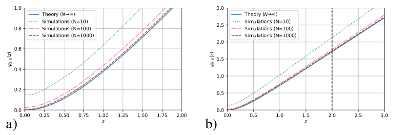
Figure 9: a) Rate function $\psi_{d,\alpha}(z)$ versus $z$, for $d=2$ and $\alpha=0$. The continuous blue line corresponds to the exact result in Eq. (56), valid in the limit $N\to\infty$. For this choice of the parameters $d$ and $\alpha$, no transition occurs. b) Rate function $\psi_{d,\alpha}(z)$ versus $z$, for $d=6$ and $\alpha=0$. The continuous blue line corresponds to the exact result in Eq. (59). The vertical dashed line signals the critical point $z_{c}$ at which the phase transition occurs, for $z>z_{c}$ the rate function becomes exactly linear. In both panels, the colored dashed lines are the results of numerical simulations obtained at finite $N$, as described in Section VII.

On the other hand, for $\nu>2$ one has

$$0<g_{d,\alpha}(-1)<+\infty\,.$$ (57)

Thus, for small positive $z$ the saddle-point equation (50) admits a unique solution $-1<q^{*}(z)<0$ and the position distribution $Z(X,N)$ is still given by the expression in Eq. (54). However, increasing $z$, the solution $q^{*}(z)$ decreases until, at the critical value $z_{c}=g_{d,\alpha}(-1)$, it encounters the branch cut at $q=-1$ (see Fig. 7). For $z>z_{c}$, $q^{*}(z)$ freezes at the value $-1$. Indeed, increasing $z$ above $z_{c}$, Eq. (50) has no solution and the integral in Eq. (49) cannot be computed via the saddle-point approximation. Nevertheless, this integral is dominated by values of $q$ close to $q=-1$ and therefore one can approximate

$$Z(X=N\,z,N)\sim\exp\left[-N\left(z-S_{d,\alpha}(-1)\right)\right]\,.$$ (58)

Hence, the rate function can be written for $\nu>2$, as

$$\psi_{d,\alpha}(z)=\begin{cases}-z~{}q^{*}(z)-S_{d,\alpha}(q^{*}(z))~{}~{}~{}~{}&\text{ for }z<z_{c}\\ \\ z-S_{d,\alpha}(-1)~{}~{}~{}~{}&\text{ for }z>z_{c}\\ \end{cases}$$ (59)

where $q^{*}(z)$ is the unique solution of Eq. (50) and

$$z_{c}=\frac{4}{d(\alpha+1)(\alpha+2)}\frac{{}_{4}F_{3}\left(\frac{3}{2},\frac{3}{2},2,2;\frac{2+d}{2},\frac{3+\alpha}{2},\frac{4+\alpha}{2};1\right)}{{}_{4}F_{3}\left(\frac{1}{2},\frac{1}{2},1,1;\frac{d}{2},\frac{1+\alpha}{2},\frac{2+\alpha}{2};1\right)}\,.$$ (60)

Note that, as expected, the critical value $z_{c}$ is the same as the one predicted by the grand canonical argument in Section III (see Eq. (34)).

For $z>z_{c}$, to find the prefactor of the expression in Eq. (58), one has to compute the contour integral in Eq. (49). We perform this calculation in the case where $\nu=(d+2\alpha-1)/2$ is not an integer for simplicity. However, this calculation can be extended easily to arbitrary $\nu$. Since we expect the integral to be dominated by values of $q$ close to $-1$, it is useful to perform the change of variable $q\to s=(q+1)N$ in Eq. (49), which yields

$$Z(X=N\,z,\,N)=\frac{1}{2\pi i}N\int_{\Gamma}ds~{}e^{N\left[(s/N-1)z+S_{d,\alpha}(-1+s/N)\right]}\,.$$ (61)

Using the asymptotic expression of the hypergeometric function close to unit argument in Eq. (52), we expand the exponent for large $N$ and we find

$$Z(X=N\,z\,N)=B_{N}e^{-Nz}\frac{1}{2\pi i}N\int_{\Gamma}ds~{}\exp\left[(z-z_{c})~{}s+a_{d,\alpha}~{}\frac{s^{2}}{N}\ldots+b_{d,\alpha}~{}\frac{s^{\nu-1}}{N^{\nu-2}}+\ldots\right]\,,$$ (62)

where $s^{\nu-1}$ is the leading singular term and

$$B_{N}=e^{NS_{d,\alpha}(-1)}\,.$$ (63)

The constants $a_{d,\alpha}$ and $b_{d,\alpha}$ can be exactly computed buhring . In particular, we find that $a_{d,\alpha}=0$ for $\nu<3$ and

$$a_{d,\alpha} = \frac{\Gamma\left(\frac{d}{2}\right)\Gamma\left(\frac{1+\alpha}{2}\right)\Gamma\left(\frac{2+\alpha}{2}\right)}{8{}_{4}F_{3}\left(\frac{1}{2},\frac{1}{2},1,1;\frac{d}{2},\frac{1+\alpha}{2},\frac{2+\alpha}{2};1\right)^{2}}\left[\frac{2~{}{}_{4}F_{3}\left(\frac{1}{2},\frac{1}{2},1,1;\frac{d}{2},\frac{1+\alpha}{2},\frac{2+\alpha}{2};1\right)}{\Gamma\left(\frac{d}{2}\right)\Gamma\left(\frac{1+\alpha}{2}\right)\Gamma\left(\frac{2+\alpha}{2}\right)}\right.\left(\frac{{}_{4}F_{3}\left(\frac{3}{2},\frac{3}{2},2,2;\frac{2+d}{2},\frac{3+\alpha}{2},\frac{4+\alpha}{2};1\right)}{\Gamma\left(\frac{2+d}{2}\right)\Gamma\left(\frac{3+\alpha}{2}\right)\Gamma\left(\frac{4+\alpha}{2}\right)}\right.$$ (64)

$$+ \left.18\frac{{}_{4}F_{3}\left[\frac{5}{2},\frac{5}{2},3,3;\frac{4+d}{2},\frac{5+\alpha}{2},\frac{6+\alpha}{2};1\right]}{\Gamma\left(\frac{4+d}{2}\right)\Gamma\left(\frac{5+\alpha}{2}\right)\Gamma\left(\frac{6+\alpha}{2}\right)}\right)-\left.\left(\frac{{}_{4}F_{3}\left(\frac{3}{2},\frac{3}{2},2,2;\frac{2+d}{2},\frac{3+\alpha}{2},\frac{4+\alpha}{2};1\right)}{\Gamma\left(\frac{2+d}{2}\right)\Gamma\left(\frac{3+\alpha}{2}\right)\Gamma\left(\frac{4+\alpha}{2}\right)}\right)^{2}\right]$$

for $\nu>3$, while

$$b_{d,\alpha}=\Gamma(1-\nu)A_{d,\alpha}\,,$$ (65)

for any $\nu$, where $A_{d,\alpha}$ is given in Eq. (33). For $\nu>3$, one can check that $a_{d,\alpha}$ is positive. Expanding Eq. (62) for large $N$ we find

$$Z(X=Nz,N)=B_{N}e^{-Nz}\frac{1}{2\pi i}N\int_{\Gamma}ds~{}e^{z_{\rm ex}s}~{}\left[1+a_{d,\alpha}~{}\frac{s^{2}}{N}\ldots+b_{d,\alpha}\frac{s^{\nu-1}}{N^{\nu-2}}+\ldots\right]\,,$$ (66)

where $z_{\rm ex}=z-z_{c}$ is assumed to be $O(1)$. It is possible to show that, for any $a\geq 0$, (see Appendix A.3 of Ref. EMZ06 )

$$\frac{1}{2\pi i}\int_{\Gamma}ds~{}e^{z_{\rm ex}s}s^{a-1}=\frac{\sin(\pi a)}{\pi}\Gamma(a)\,.$$ (67)

Thus, when $a$ is integer, the integral above vanishes. Therefore, since we are assuming that $\nu$ is not an integer, the leading term in Eq. (66) is, using the expression for $b_{d,\alpha}$ given in Eq. (65),

$$Z(X=Nz,N)\simeq B_{N}e^{-Nz}\frac{1}{z_{\rm ex}^{\nu}}\frac{b_{d,\alpha}}{N^{\nu-1}}\frac{\sin(\pi\nu)}{\nu}\Gamma(\nu)\Gamma(1-\nu)A_{d,\alpha}\,.$$ (68)

Finally, using the relation $\Gamma(\nu)\Gamma(1-\nu)=\pi/\sin(\nu\pi)$, we find

$$Z(X,N)\simeq B_{N}A_{d,\alpha}\frac{N}{(X-X_{c})^{\nu}}e^{-X}\,.$$ (69)

When $\nu$ is an integer, a similar argument can be applied. Note that the expression in Eq. (69) can be rewritten, using the large-$x$ expansion of $p(x)$ in Eq. (32), as

$$Z(X,N)\simeq C_{N}Np(X-X_{c})\,,$$ (70)

where $p(x)$ is the PDF of a single-run displacement and $C_{N}=B_{N}e^{-X_{c}}$. This expression can be interpreted as follows. Above the critical value $X=X_{c}$, all the extra displacement $X_{\rm ex}=X-X_{c}$ is absorbed by a single run, the condensate. The probability weight associated to the condensate is therefore $p(X-X_{c})$ and the factor $N$ in Eq. (70) arises since the condensate can be any one of the $N$ runs. The factor $C_{N}$ in Eq. (49) is the probability weight of the other $N-1$ sites, which becomes independent of $X$ above the transition.

IV.3 Order of the transition

It is also interesting to compute the order of the phase transition described above. We recall that the system undergoes a transition of order $n$ if the $n$-th derivative of $\psi_{d,\alpha}(z)$ is discontinuous, while all lower-order derivatives are continuous. Thus, we need to investigate the asymptotic behavior of $\psi_{d,\alpha}(z)$ close to the transition. In the limit $z\to z_{c}$ from below, we know that a solution $q^{*}(z)$ of the saddle point equation always exists. Moreover, since we know that exactly at the critical point $z=z_{c}$ the saddle point $q^{*}(z)$ encounters the branch cut at $q=-1$, we expect that $q^{*}(z)$ is close to $-1$ near the transition. Plugging $q=-1+s$ into the exponent of the integrand in Eq. (49) and using Eq. (52) to expand for small $s$, we obtain

$$z~{}q+S_{d,\alpha}(q)\simeq S_{d,\alpha}(-1)-z+z_{\rm ex}s+c_{\nu}\,s^{\eta}\,,$$ (71)

where $c_{\nu}=b_{d,\alpha}$ for $2<\nu<3$ and $c_{\nu}=a_{d,\alpha}$ for $\nu>3$ (where $a_{d,\alpha}$ and $b_{d,\alpha}$ are given in Eqs. (64) and (65)), and

$$\eta=\begin{cases}\nu-1&\text{for }2<\nu<3,\\ \\ 2&\text{for }\nu>3.\\ \end{cases}$$ (72)

We recall that $S_{d,\alpha}(q)$ is defined in Eq. (44). Setting to zero the first derivative with respect to $s$ of the expression in Eq. (71), we obtain

$$s=\left(\frac{z_{c}-z}{c_{\nu}~{}\eta}\right)^{1/(\eta-1)}\,.$$ (73)

Thus, the saddle point is located at, for $z\to z_{c}$,

$$q^{*}(z)\simeq-1+\left(\frac{z_{c}-z}{c_{\nu}~{}\eta}\right)^{1/(\eta-1)}\,.$$ (74)

Plugging this value into Eq. (59), we find that when $z\to z_{c}$ from below

$$\psi_{d,\alpha}(z)\simeq z-S_{d,\alpha}(-1)+\left((c_{\nu}~{}\eta)^{-1/(\eta-1)}-\frac{c_{\nu}}{(c_{\nu}~{}\eta)^{\eta/(\eta-1)}}\right)~{}(z_{c}-z)^{\eta/(\eta-1)}\,.$$ (75)

Recalling that for $z>z_{c}$

$$\psi_{d,\alpha}(z)=z-S_{d,\alpha}(-1)\,,$$ (76)

we find that the order $n$ of the transition is $\left\lceil\eta/(\eta-1)\right\rceil$, where $\left\lceil y\right\rceil$ denotes the smallest integer larger than or equal to $y$. Using the expression for $\eta$ given in Eq. (72), we find

$$n=\begin{cases}\left\lceil\frac{\nu-1}{\nu-2}\right\rceil&\text{for }2<\nu<3,\\ \\ 2&\text{for }\nu>3.\\ \end{cases}$$ (77)

In other words, we observe a second-order phase transition for $\nu>3$, while, for $2<\nu<3$, the order of the transition depends continuously on $\nu$. For instance, when $\nu=5/2$ we find $n=3$. Notably, the order $n$ diverges when $\nu\to 2$, in agreement with the fact that for $\nu=2$ all derivatives of $\psi_{d,\alpha}(z)$ are continuous.

IV.4 Asymptotics of $\psi_{d,\alpha}(z)$

Next, we are interested in the asymptotic behavior of $\psi_{d,\alpha}(z)$ for small and large $z$. For small enough $z$, a solution of the saddle point equation (50) always exists, with $q^{*}(z)$ small. Expanding Eq. (50) for small $q^{*}(z)$, we find

$$q^{*}(z)\simeq-\frac{d(\alpha+1)(\alpha+2)}{4}z.$$ (78)

Plugging this solution into Eq. (55) and expanding for small $z$, we obtain

$$\psi_{d,\alpha}(z)\simeq\frac{d(1+\alpha)(2+\alpha)}{8}z^{2}\,.$$ (79)

Comparing this result with Eq. (11), we notice that the small-argument behavior of the rate function smoothly connects with the typical Gaussian behavior in Eq. (11). We next consider the large-$z$ behavior of $\psi_{d,\alpha}(z)$. It is useful to distinguish different cases, depending on $\nu$.

The case $\nu>2$: For $\nu>2$, we already know that for $z>z_{c}$ the rate function is exactly given by just a linear function

$$\psi_{d,\alpha}(z)=z-S_{d,\alpha}(-1)\,,$$ (80)

where $S_{d,\alpha}(q)$ is given in Eq. (44).

The case $1<\nu<2$: When $\nu<2$, for large $z$, we know that a unique solution $q^{*}(z)$ of the saddle point Eq. (50) exists for any $z$. Moreover, in the limit of large $z$, we expect $q^{*}(z)$ to be close to $-1$. Therefore, we plug $q=-1+s$ into the exponent of the integrand in Eq. (49) and we use Eq. (52) to expand for small $s$. For $1<\nu<2$, we obtain

$$z~{}(-1+s)+S_{d,\alpha}(-1+s)\simeq z(-1+s)+S_{d,\alpha}(-1)+\tilde{a}s^{\nu-1}\,,$$ (81)

where $\tilde{a}<0$ is a constant that depends on $d$ and $\alpha$. Setting to zero the first derivative of this expression with respect to $s$, we obtain

$$z+\tilde{a}(\nu-1)s^{\nu-2}=0\,.$$ (82)

Thus, we find that, for large $z$, the solution of the saddle point equation can be written as

$$q^{*}(z)\simeq-1+(\tilde{a}(1-\nu)/z)^{1/(2-\nu)}\,.$$ (83)

Plugging this expression for $q^{*}(z)$ into Eq. (55) and expanding for large $z$, we finally obtain

$$\psi_{d,\alpha}(z)=z-S_{d,\alpha}(-1)+O(z^{(1-\nu)/(2-\nu)})\,.$$ (84)

The case $0<\nu<1$: When $0<\nu<1$ the procedure above yields, to leading order in $s$,

$$z~{}(-1+s)+S_{d,\alpha}(-1+s)\simeq z(-1+s)+(\nu-1)\log\left(s\right)\,.$$ (85)

Setting to zero the first derivative of this expression with respect to $s$, we find that the saddle point equation becomes, for $z\gg 1$,

$$z+\frac{\nu-1}{s}=0\,.$$ (86)

Thus, we find that, to leading order, $q^{*}(z)\simeq-1+(1-\nu)/z$. Plugging this expression in Eq. (55) and expanding for large $z$, we find that, for $0<\nu<1$,

$$\psi_{d,\alpha}(z)=z-(1-\nu)\log(z)+O(1)\,.$$ (87)

To summarize, we have shown that, for $z\gg 1$,

$$\psi_{d,\alpha}(z)=\begin{cases}z-(1-\nu)\log(z)+O(1)&\text{for }0<\nu<1\\ \\ z-S_{d,\alpha}(-1)+O(z^{(1-\nu)/(2-\nu)})&\text{for }1<\nu<2\\ \\ \\ z-S_{d,\alpha}(-1)&\text{for }\nu>2\,,\\ \\ \end{cases}$$ (88)

where we recall that $S_{d,\alpha}(q)$ is given in Eq. (44).

IV.5 Vicinity of the critical point: intermediate matching regime

We now focus on the case $\nu>2$ where a condensation is guaranteed to occur as $X$ exceeds a critical value $X_{c}$. We want to investigate the behavior of $Z(X,N)$ in a small neighborhood of the critical point $X=X_{c}$ for large $N$ (see Fig. 2). In the following, we will assume that $\nu$ is not an integer number. The discussion below can be easily generalized to the case where $\nu$ is integer. We recall that $X_{c}=z_{c}N$, where the critical value $z_{c}$, given in Eq. (60), is of order one. Close to the transition, we write $X$ as

$$X=X_{c}+yN^{\lambda}\,,$$ (89)

where $y$ is an order-one variable and $0<\lambda<1$ can be adjusted depending on $\nu$. Close to the transition, i.e. for $|X_{\rm ex}|=|X-X_{c}|\ll N$, we know that the contour integral in Eq. (49) is dominated by values of $q$ close to $-1$. Thus, performing the change of variable $q\to s=-1+q$, we find

$$Z(X,N)=\frac{1}{2\pi i}\int_{\Gamma}ds~{}e^{(-1+s)X+N~{}S_{d,\alpha}(-1+s)}\,,$$ (90)

where $S_{d,\alpha}(q)$ is given in Eq. (44). Using Eq. (52), we expand for small $s$ and we obtain

$$Z(X,N)\simeq B_{N}~{}e^{-X}\frac{1}{2\pi i}\int_{\Gamma}ds~{}\exp\left[(X-X_{c})s+N\left(a_{d,\alpha}~{}s^{2}+\ldots+b_{d,\alpha}~{}s^{\nu-1}+\ldots\right)\right]\,,$$ (91)

where $s^{\nu-1}$ is the first non-analytic term of the expansion and $B_{N}$ is given in Eq. (63). The constants $a_{d,\alpha}$ and $b_{d,\alpha}$ are given in Eqs. (64) and (65). Using Eq. (89), we obtain

$$Z(X,N)\simeq B_{N}e^{-X}\frac{1}{2\pi i}\int_{\Gamma}ds~{}\exp\left[ysN^{\lambda}+N\left(a_{d,\alpha}~{}s^{2}+\ldots+b_{d,\alpha}~{}s^{\nu-1}+\ldots\right)\right]\,.$$ (92)

After the change of variable $s\to\tilde{s}=sN^{\lambda}$, we get

$$Z(X,N)\simeq B_{N}e^{-X}\frac{N^{-\lambda}}{2\pi i}\int_{\Gamma}d\tilde{s}~{}\exp\left[y\tilde{s}+a_{d,\alpha}~{}\tilde{s}^{2}N^{1-2\lambda}+\ldots+b_{d,\alpha}~{}\tilde{s}^{\nu-1}N^{1-(\nu-1)\lambda}+\ldots\right]\,.$$ (93)

Let us now consider the two cases $2<\nu<3$ and $\nu>3$ separately.

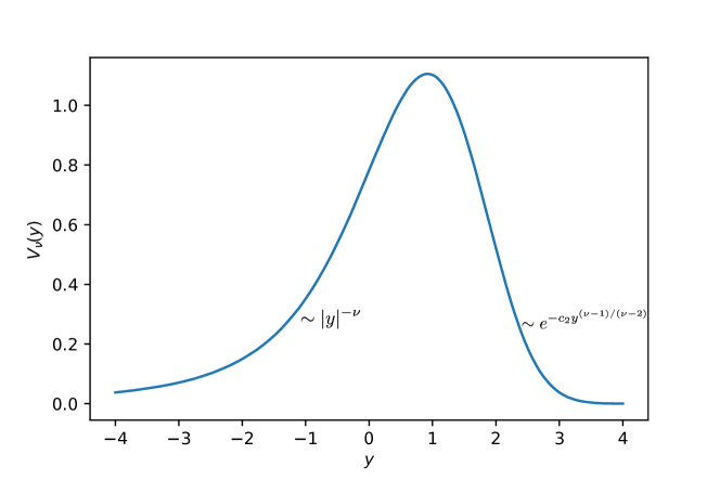
Figure 10: The function $V_{\nu}(y)$ versus $y$, for $\nu=5/2$. For $y\to\infty$, $V_{\nu}(y)$ decays exponentially fast as $e^{-c_{2}y^{(\nu-1)/(\nu-2)}}$. For $y\to-\infty$, it has a power-law tail $V_{\nu}(y)\sim|y|^{-\nu}$.

For $2<\nu<3$, we set $\lambda=1/(\nu-1)$ and, using the definition of $y$ in Eq. (89), we obtain, to leading order,

$$Z(X,N)\simeq C_{N}\frac{1}{N^{1/(\nu-1)}}V_{\nu}\left(\frac{X_{c}-X}{N^{1/(\nu-1)}}\right)\,,$$ (94)

where $C_{N}=B_{N}e^{-X}$ and

$$V_{\nu}(y)=\frac{1}{2\pi i}\int_{\Gamma}ds~{}\exp\left[-y~{}s+b_{d,\alpha}~{}s^{\nu-1}\right]\,.$$ (95)

This same function $V_{\nu}(y)$ also appeared in the analysis of the partition function in mass transport models EMZ06 ; EM08 and is shown in Fig. 10. It has the following asymptotic behaviors EMZ06

$$V_{\nu}(y)\simeq\begin{cases}A_{d,\alpha}|y|^{-\nu}&\text{ for }y\to-\infty\\ \\ c_{1}~{}y^{(3-\nu)/(2(\nu-2))}e^{-c_{2}~{}y^{(\nu-1)/(\nu-2)}}&\text{ for }y\to\infty\,,\end{cases}$$ (96)

where $A_{d,\alpha}$ is given in Eq. (33),

$$c_{1}=\frac{1}{\left(2\pi(\nu-2)(b_{d,\alpha}(\nu-1))^{1/(\nu-2)}\right)^{1/2}}$$ (97)

and

$$c_{2}=\frac{\nu-2}{(\nu-1)(b_{d,\alpha}(\nu-1))^{1/(\nu-2)}}\,.$$ (98)

Performing the change of variable $s=re^{\pm i\pi/2}$ for the upper and lower part of the imaginary-axis contour $\Gamma$, it is possible to rewrite the expression for $V_{\nu}(y)$ in Eq. (95) as

$$V_{\nu}(y)=\frac{1}{\pi}\int_{0}^{\infty}dr~{}e^{b_{d,\alpha}\sin(\pi\nu/2)r^{\nu-1}}\cos\left[b_{d,\alpha}\cos(\pi\nu/2)r^{\nu-1}+yr\right]\,,$$ (99)

which can be easily evaluated numerically. Moreover, it is easy to check that $V_{\nu}(y)$ is positive and normalized to one. Using the asymptotic result for $y\to\infty$, one can check that the expression for $Z(X,N)$ in Eq. (94) matches smoothly to the expression obtained by saddle-point approximation for $z<z_{c}$ (see Eq. (75)). Similarly, using the expansion for $y\to-\infty$, we observe that for $X_{\rm ex}=X-X_{c}\gg N^{1/(\nu-1)}$

$$Z(X,N)\simeq B_{N}e^{-X}\frac{N~{}A_{d,\alpha}}{(X-X_{c})^{\nu}}\,,$$ (100)

in agreement with the result in Eq. (69).

When $\nu>3$, we set $\lambda=1/2$ in Eq. (93) and we obtain

$$Z(X,N)\simeq B_{N}e^{-X}\frac{N^{-1/2}}{2\pi i}\int_{\Gamma}d\tilde{s}~{}\exp\left[y\tilde{s}+a_{d,\alpha}~{}\tilde{s}^{2}\right]\,.$$ (101)

Computing the integral over $\tilde{s}$ and using the definition of $y$, we get

$$Z(X,N)\simeq C_{N}\frac{1}{\sqrt{4\pi a_{d,\alpha}N}}\exp\left[-\frac{\left(X-X_{c}\right)^{2}}{4a_{d,\alpha}N}\right]\,,$$ (102)

where $C_{N}=B_{N}e^{-X_{c}}$. Thus, for $\nu>3$ the PDF of $X$ has, in the critical region where $|X-X_{c}|\sim\sqrt{N}$, a Gaussian shape. Actually, it is possible to check that this Gaussian form remains valid, on the left tail, on a larger region, depending on $\nu$. For instance, for $\nu>4$, it is valid up to $X_{c}-X\sim N^{3/4}$. Conversely, on the right tail, the expression in Eq. (102) remains valid up to $X-X_{c}\sim\sqrt{N\log(N)}$. Beyond this scale, i.e., for $X-X_{c}\gg\sqrt{N\log(N)}$, it is possible to show that

$$Z(X,N)\simeq B_{N}e^{-X}\frac{N~{}A_{d,\alpha}}{(X-X_{c})^{\nu}}\,,$$ (103)

in agreement with the expression in Eq. (69), obtained for $X-X_{c}\sim O(N)$.

In order to describe the crossover between the Gaussian shape in Eq. (102) and the power-law tail in Eq. (103), one needs to keep the first singular term in the expansion in Eq. (101). From Eq. (93), we obtain

$$Z(X,N)\simeq B_{N}e^{-X}\frac{N^{-1/2}}{2\pi i}\int_{\Gamma}d\tilde{s}~{}\exp\left[y\tilde{s}+a_{d,\alpha}~{}\tilde{s}^{2}+b_{d,\alpha}\tilde{s}^{\nu-1}N^{-(\nu-3)/2}\right]\,.$$ (104)

For large $N$, the integrand can be written as

$$Z(X,N)\simeq B_{N}e^{-X}\frac{1}{\sqrt{N}}~{}g_{N}\left(\frac{X-X_{c}}{\sqrt{N}}\right)\,,$$ (105)

where

$$g_{N}(y)=\frac{1}{2\pi i}\int_{\Gamma}ds~{}e^{ys+a_{d,\alpha}s^{2}}\left(1+b_{d,\alpha}s^{\nu-1}N^{-(\nu-3)/2}\right)\,.$$ (106)

This function $g_{N}(y)$ can be rewritten as the sum of a Gaussian part and of power-law part

$$g_{N}(y)=\frac{1}{\sqrt{4\pi a_{d,\alpha}}}e^{-y^{2}/(4a_{d,\alpha})}+\frac{b_{d,\alpha}}{N^{(\nu-3)/2}}\frac{1}{2\pi i}\int_{\Gamma}ds~{}e^{ys+a_{d,\alpha}s^{2}}s^{\nu-1}\,.$$ (107)

When $y\sim O(1)$, the Gaussian term is always leading and one obtains the result in Eq. (102). On the other hand, when $y\sim O(\sqrt{N})$, the power-law part dominates, coherently with the result in Eq. (103). We now want to describe the crossover between these two regimes. When $y\gg 1$ the integral over $s$ can be approximated as

$$g_{N}(y)\simeq\frac{1}{\sqrt{4\pi a_{d,\alpha}}}e^{-y^{2}/(4a_{d,\alpha})}+\frac{A_{d,\alpha}}{N^{(\nu-3)/2}}\frac{1}{y^{\nu}}\,,$$ (108)

where we have used the expression for $b_{d,\alpha}$, given in Eq. (33). We want to find $c_{N}$ and $d_{N}$, such that $w=(y-c_{N})/d_{N}$ is fixed for large $N$. Plugging

$$y=c_{N}+d_{N}w$$ (109)

in Eq. (108), we obtain

$$g_{N}(y=c_{N}+d_{N}w)=\frac{A_{d,\alpha}}{N^{(\nu-3)/2}}\frac{1}{c_{N}^{\nu}(1+d_{N}w/c_{N})^{\nu}}\left[1+\frac{N^{(\nu-3)/2}c_{N}^{\nu}(1+d_{N}w/c_{N})^{\nu}}{\sqrt{4\pi a_{d,\alpha}}~{}A_{d,\alpha}}e^{-(c_{N}^{2}+2c_{N}d_{N}w+d_{N}^{2}w^{2})/(4a_{d,\alpha})}\right]\,.$$ (110)

We now choose $c_{N}$ such that

$$N^{(\nu-3)/2}c_{N}^{\nu}e^{-c_{N}^{2}/(4a_{d,\alpha})}=1\,.$$ (111)

Thus, to leading order

$$c_{N}\simeq\sqrt{2a_{d,\alpha}(\nu-3)\log(N)}\,.$$ (112)

Moreover, we choose $d_{N}=1/c_{N}$. Then, to leading order, we obtain

$$g_{N}(y=c_{N}+d_{N}w)=\frac{A_{d,\alpha}}{N^{(\nu-3)/2}}\frac{1}{(2a_{d,\alpha}(\nu-3)\log(N))^{\nu/2}}\left[1+\frac{1}{\sqrt{4\pi a_{d,\alpha}}~{}A_{d,\alpha}}e^{-w/(2a_{d,\alpha})}\right]\,.$$ (113)

Finally, using Eq. (105), we find that

$$Z(X,N)\simeq B_{N}\frac{A_{d,\alpha}}{c_{N}^{\nu}N^{(\nu-3)/2}}e^{-X}~{}h\left[c_{N}\left(\frac{X-X_{c}}{\sqrt{N}}-c_{N}\right)\right]\,,$$ (114)

where $c_{N}$ is given in Eq. (112) and

$$h(w)=1+\frac{1}{\sqrt{4\pi a_{d,\alpha}}~{}A_{d,\alpha}}e^{-w/(2a_{d,\alpha})}\,.$$ (115)

Overall, we have shown that the crossover occurs for $X-X_{c}\sim\sqrt{N\log(N)}$ and that it is described by the function $h(w)$.

To summarize, we have shown that, for any $\nu>2$ and for $X\sim X_{c}$, the PDF $Z(X,N)$ can be always written as

$$Z(X,N)\simeq C_{N}p_{\rm cond}(X_{c}-X,N)\,,$$ (116)

where the function $p_{\rm cond}(y,N)$ assumes different expressions depending on $\nu$. The reason behind the choice of the subscript cond will become clear in the next section. Using Eq. (94), we find that for $2<\nu<3$

$$p_{\rm cond}(y,N)\simeq\frac{1}{N^{1/(\nu-1)}}V_{\nu}\left(\frac{y}{N^{1/(\nu-1)}}\right)\,,$$ (117)

where the function $V_{\nu}(y)$ in Eq. (95). On the other hand, for $\nu>3$, we find

$$p_{\rm cond}(y,N)\simeq\begin{cases}\frac{NA_{d,\alpha}}{|y|^{\nu}}~{}~{}~{}&\text{ for }y\ll-\sqrt{N\log(N)}~{},\\ \\ \frac{A_{d,\alpha}}{c_{N}^{\nu}N^{(\nu-3)/2}}h\left[\frac{c_{N}}{\sqrt{N}}\left(|y|-\sqrt{N}c_{N}\right)\right]~{}~{}~{}&\text{ for }y\simeq-\sqrt{N\log(N)}~{},\\ \\ \frac{1}{\sqrt{4\pi a_{d,\alpha}N}}e^{-y^{2}/(4a_{d,\alpha}N)}~{}~{}~{}&\text{ for }y\gg-\sqrt{N\log(N)}\,,\end{cases}$$ (118)

where $A_{d,\alpha}$ and $a_{d,\alpha}$ are given in Eqs. (33) and (64). The function $h(w)$ is given in Eq. (115) and $c_{N}\sim\sqrt{\log(N)}$ is given in Eq. (112). In both cases, it is possible to check that the function $p_{\rm cond}(y,N)$ is positive and normalized over $y$, for large $N$. Using Eqs. (117) and (118), we find that for $y\to\infty$

$$p_{\rm cond}(y,N)\sim\begin{cases}\exp\left[-c_{2}\frac{y^{(\nu-1)/(\nu-2)}}{N^{1/(\nu-2)}}\right]~{}~{}~{}&\text{ for }2<\nu<3~{},\\ \\ \exp\left[-\frac{y^{2}}{4a_{d,\alpha}N}\right]~{}~{}~{}&\text{ for }\nu>3\,,\end{cases}$$ (119)

where $c_{2}$ is given in Eq. (98). On the other hand, for $y\to-\infty$, we obtain

$$p_{\rm cond}(y,N)\simeq\frac{NA_{d,\alpha}}{|y|^{\nu}}\,,$$ (120)

for any $\nu>2$.

V Marginal distribution of a single jump

In this section we investigate the marginal PDF $p(x|X)$ of a single-run displacement $x$, conditioned on the final $x$-component displacement $X$. This means that if we pick at random one of the $N$ runs with the total displacement $X$ fixed, what is the distribution of the size of this run? Note that the displacements $x_{1}\,,\ldots\,,x_{N}$ are i.i.d. random variables, since we are considering the fixed-$N$ ensemble. Thus, $x$ can be identified with any of these variables, say for simplicity $x=x_{1}$. Then, the conditional PDF of $x$ is given by

$$p(x|X)=\frac{p(x)\int_{-\infty}^{\infty}dx_{2}~{}\ldots\int_{-\infty}^{\infty}dx_{N}\left[\prod_{i=2}^{N}p(x_{i})\right]\delta\left(X-x-\sum_{i=2}^{\infty}x_{i}\right)}{\int_{-\infty}^{\infty}dx_{1}~{}\ldots\int_{-\infty}^{\infty}dx_{N}\left[\prod_{i=1}^{N}p(x_{i})\right]\delta\left(X-\sum_{i=1}^{\infty}x_{i}\right)}\,,$$ (121)

which can be rewritten as

$$p(x|X)=p(x)~{}\frac{Z(X-x,N-1)}{Z(X,N)}\,,$$ (122)

where we have used the definition of $Z(X,N)$ in Eq. (3). We are interested in the large-deviation regime where $X=zN$ and $z$ is of order one. As explained in the previous section, for $\nu>2$, the system undergoes a phase transition at a critical value $z_{c}$ of the parameter $z$. In this section we show that this transition shows up very clearly in the marginal distribution $p(x|X)$ which has very different behavior in the subcritical ($X<z_{c}N$) and the supercritical ($X>z_{c}N$) phases. In the subcritical ‘fluid’ phase, $p(x|X)$ is a monotonically decreasing function of $x$ with an exponential tail. For $X=z_{c}N$ we have a critical fluid where $p(x|X)$ still decays monotonically with increasing $x$, but now as a power law $\sim x^{-\nu}$ for large $x$. Finally, in the supercritical phase ($X>z_{c}N$), $p(x|X)$ becomes non-monotonic as a function of $x$, developing in particular a bump centered at $x=X_{\rm ex}=X-z_{c}N$ (see Fig. 3). Let us discuss these three cases separately.

Subcritical phase ($X<X_{c}$): Plugging the expression for $Z(X,N)$ given in Eq. (49), into Eq. (122), we obtain

$$p(x|X)\simeq p(x)~{}\frac{\int_{\Gamma}dq~{}e^{-qx}e^{N\left[qz+S_{d,0}(q)\right]}}{\int_{\Gamma}dq~{}e^{N\left[qz+S_{d,0}(q)\right]}}\,,$$ (123)

where the integrals are performed over the imaginary-axis Bromwich contour $\Gamma$ (see Fig. 7). In Section IV, we have shown that the integrals above are dominated by the solution $q^{*}(z)$ of the saddle point equation (50). In the subcritical phase $z<z_{c}$ such solution $q^{*}(z)>-1$ always exists. Thus, from Eq. (123), we obtain

$$p(x|X)\simeq p(x)e^{-q^{*}(z)\,x}\,.$$ (124)

Using the large-$x$ behavior of $p(x)$, given in Eq. (32), we find that, for $x\gg 1$

$$p(x|X)\simeq A_{d,\alpha}x^{-\nu}~{}e^{-x/\xi}\,,$$ (125)

where

$$\xi=\frac{1}{1+q^{*}(z)}\,.$$ (126)

Thus for $X<X_{c}$, the PDF $p(x|X)$ decays as a function of $x$ on a typical length $\xi>0$. Recalling that $q^{*}(z)\to-1$ for $z\to z_{c}$, we find that $\xi$ diverges when the system approaches the phase transition. In particular, it is possible to show that $\xi$ diverges, for $z\to z_{c}$ from below, as

$$\xi\sim\begin{cases}(z_{c}-z)^{-1/(\nu-2)}&\text{ for }2<\nu<3\\ \\ (z_{c}-z)^{-1/2}&\text{ for }\nu>3\,.\\ \end{cases}$$ (127)

Critical phase ($X=X_{c}$): Exactly at the transition point, the typical length $\xi$ diverges and therefore the single-jump distribution develops a power-law tail for large $x$

$$p(x|X)\simeq A_{d,\alpha}x^{-\nu}\,.$$ (128)

Note that the result in Eq. (128) is only valid for $x\ll O(N)$. This is because when computing the integral in Eq. (123) we have assumed that the factor $e^{-qx}$ does not contribute to the saddle point equation, which is only true if $x\ll O(N)$. As we will show below, configurations with $x\sim O(N)$ are exponentially rare when $X=X_{c}$.

We note that the behavior of our system in the subcritical phase and at the critical point is somewhat reminiscent of a standard phase transition such as in the Ising model in $d\geq 2$. The subcritical phase “corresponds” to the paramagnetic phase of the Ising model. The marginal distribution $p(x|X)$ plays an “analogous” role as the spin-spin correlation function in the Ising model. In the case of the Ising model, the correlation function decays exponentially with distance with a characteristic correlation length that diverges as one approaches the critical point. Similarly, here there is a characteristic run length $\xi$ characterizing the exponential decay of $p(x|X)$ with $x$ on the subcritical side, with $\xi$ diverging as one approaches the critical point.

Supercritical phase ($X=X_{c}$): Above the transition, $q^{*}(z)$ freezes to the value $-1$ and therefore the typical length $\xi$ remains infinite. Indeed, for $X>X_{c}$, we expect that the condensate develops as a bump in the tail of the PDF $p(x|X)$. The location of this bump is related to the fraction of $X$ that is contained in the condensate. Moreover, the area under the bump is the probability that a particular single-run displacement becomes the condensate. In the presence of a single condensate, this area should therefore be $1/N$. Finally, as we will show, the shape of the bump is related to the order of the phase transition. Since we expect the condensate to contain a finite fraction of $X$, we need to investigate configurations where $x\sim O(N)$. Thus, it is useful to define the scaled variable $y=x/N$, which is of order one when $x\sim O(N)$, and to rewrite $p(x|X)$ as

$$p(x=yN|X=zN)=p(yN)~{}\frac{Z(N(z-y),N-1)}{Z(Nz,N)}\,.$$ (129)

Let us first investigate the exponential part of $p(x|X)$.

Plugging the large-deviation form of $Z(X,N)$, given in Eq. (54) and the large-$x$ behavior of $p(x)$, given in Eq. (32), into Eq. (129), we find

$$p(x|X)\sim\exp\left[-N\chi\left(\frac{x}{N},\frac{X}{N}\right)\right]\,,$$ (130)

where

$$\chi(y,z)=\psi_{d,\alpha}(z-y)+y-\psi_{d,\alpha}(z)\,,$$ (131)

and $\psi_{d,\alpha}(z)$ is given in Eq. (59). Thus, in the regime where $x\sim O(N)$, the PDF $p(x|X)$ assumes a large deviation form with rate function $\chi(y,z)$. The rate function $\chi(y,z)$ is shown in Fig. 11 as a function of $y$, for different values of $z$.

Using the expression of $\psi_{d,\alpha}(z)$ in Eq. (59), it is easy to show that, for $y>z_{\rm ex}$, one has $\chi(y,z)>0$, where we recall that $z_{\rm ex}=z-z_{c}$ (see Fig. 11). Thus, configurations where $x>X_{\rm ex}$ become exponentially rare for large $x$. On the other hand, for $y<z_{\rm ex}$, we find that $\chi(y,z)=0$. This means that configurations with $y<z_{\rm ex}$ are not forbidden and that a bump can arise in the tail of $p(x|X)$. Note however that where $\chi(y,z)=0$ the large-deviation description fails and that we need to carefully consider the full distribution, and not just the exponential part.

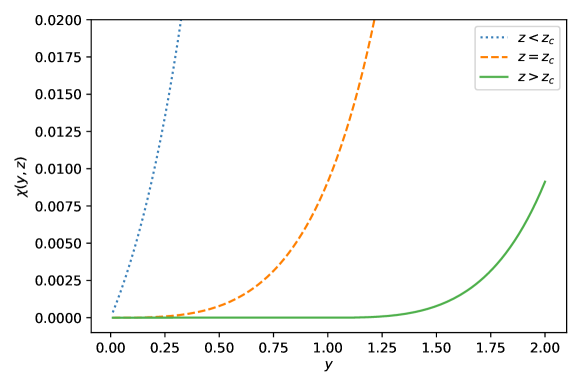
Figure 11: Rate function $\chi(y,z)$ versus $y$, for different values of $z$. The curves are obtained from the exact result in Eq. (131), for $d=6$ and $\alpha=0$. For $z<z_{c}$, we observe that $\chi(y,z)>0$ for any $y>0$. Conversely, for $z>z_{c}$, the rate function $\chi(y,z)$ vanishes for $y<z_{\rm ex}=z-z_{c}$ (in this case $z_{\rm ex}=1$).

Therefore, we focus on the region $0<y<z_{\rm ex}$, where we have just shown that the exponential part of the distribution of $p(x|X)$ vanishes. We use the expression in Eq. (69) to approximate both the numerator and the denominator of Eq. (129). Using also the asymptotic expression of $p(x)$ for large $x$, given in Eq. (32), we obtain

$$p(x|X)\simeq\frac{A_{d,\alpha}}{N^{\nu}y^{\nu}}\frac{1}{(1-y/z_{\rm ex})^{\nu}}\,,$$ (132)

where $A_{d,\alpha}$ is given in Eq. (33) and we recall that $z_{\rm ex}=z-z_{c}$. Going back to the original variables $x=y/N$ and $X=z/N$, we find that in the regime where both $x$ and $X$ scale linearly with $N$, with $0<x<X_{\rm ex}$,

$$p(x|X)\simeq\frac{A_{d,\alpha}}{x^{\nu}}\frac{1}{(1-x/X_{\rm ex})^{\nu}}\,.$$ (133)

Note that this approximate expression breaks down when $x\to X_{\rm ex}$. As we will see, at $x\sim X_{\rm ex}$ the condensate bump appears in the tail of the distribution of $p(x|X)$.

Let us now focus on the region where $x\sim X_{\rm ex}$, where we expect the bump to appear. In this region, the numerator of Eq. (129) can be approximated using the expression in Eq. (116). On the other hand, the denominator can be approximated with the expression in Eq. (69). Using also the large-$x$ expansion of $p(x)$, given in Eq. (32), we obtain, to leading order

$$p(x|X)\simeq\frac{1}{N}p_{\rm cond}(x-X_{\rm ex},N)\,,$$ (134)

where $p_{\rm cond}(y,N)$ is given in Eq. (16) for $2<\nu<3$ and in Eq. (17) for $\nu>3$. Thus, for $z>z_{c}$, a condensate bump appears at $x\sim X_{\rm ex}$. For $2<\nu<3$, the condensate bump has an anomalous shape described by the function $V_{\nu}(y)$ in Eq. (95), with fluctuations of order $O(N^{1/(\nu-1)})$. For $\nu>3$, the condensate has a Gaussian shape in the vicinity of its peak, with fluctuations of order $O(\sqrt{N})$. In both cases, we observe that the bump width vanishes relative to its location, since $X_{\rm ex}\sim O(N)$. Moreover, the area under the bump corresponds to the probability that the condensate appears in a particular running-phase. Since $p_{\rm cond}(y,N)$ is normalized to one, we find that this area is $1/N$, signaling the presence of a single condensate. The results above are summarized in Fig. 4 and are in agreement with the numerical simulations, presented in Fig. 3. The asymptotic behaviors of $p_{\rm cond}(y,N)$ are given in Eqs. (119) and (120).

Finally, it is also instructive to investigate the condensate fraction $m_{c}$, defined as the fraction of the total displacement that is carried by the condensate. In this section we have shown that, for $\nu>2$, the condensate is located at $x=X_{\rm ex}$, with sublinear fluctuations around this value. Thus, for $N\to\infty$, the condensate fraction converges to

$$m_{c}=\frac{X-X_{c}}{X}\,,$$ (135)

or, in terms of the scaled variable $z$,

$$m_{c}=\frac{z-z_{c}}{z}\,.$$ (136)

This quantity $m_{c}$ is the natural order parameter of the system, with $z$ being the corresponding control parameter. Indeed, for $z<z_{c}$ no condensate can form and thus $m_{c}=0$. On the other hand, above the transition, the condensate fraction becomes positive.

VI Fixed-$T$ ensemble

In this section, we consider a single RTP in the fixed-$T$ ensemble. As explained in Section II, according to this alternative model, the total duration $T$ of the RTP trajectory is fixed and the number $N$ of running phases is a random variable. While the fixed-$N$ ensemble can be easily mapped into a discrete-time random walk, the fixed-$T$ ensemble is a truly continuous-time process and is often taken as the standard model for RTPs. The goal of this section is to show that the results of this paper can be extended also to the fixed-$T$ ensemble. The technique that we apply in the following is based on a mapping of the continuous-time trajectory of the RTP to a discrete-time random walk in Laplace space. This method has been used to compute several observables, e.g. the survival probability, of a fixed-$T$ RTP MLDM20a ; MLDM20 ; BMS2021 ; LM20 . For the sake of simplicity, we will henceforth focus on the model where the speed $v_{0}$ of the particle is kept fixed. We recall that this corresponds to taking the limit $\alpha\to 0$. It is easy to extend the computations of this section to generic $\alpha>0$.

By definition, we consider the starting point to be a tumbling event, thus $N\geq 1$ indicates also the total number of tumblings. Let us denote by $\tau_{i}$ the duration of the $i$-th running phase, i.e., the running phase after the $i$-th tumbling. We also recall that $x_{i}$ denotes the $x$-component displacement of the particle during the $i$-th running phase. Since we are assuming that the tumblings happen with a constant rate $\gamma$, for the first $N-1$ running phases the PDF of $\tau_{i}$ is given by

$$P(\tau_{i})=\gamma e^{-\gamma\tau_{i}}\,.$$ (137)

However, since we are fixing the total time $T$, the last running phase $\tau_{N}$ is yet to be completed and thus its probability weight is given by

$$P(\tau_{N})=\int_{\tau_{N}}^{\infty}dt\,\gamma~{}e^{-\gamma t}=e^{-\gamma\tau_{N}}\,.$$ (138)

Thus, the joint probability of the running times $\{\tau_{i}\}=\tau_{1}\,,\ldots,\tau_{N}$ and of the number $N$ of tumblings, fixing the total time $T$, is given by

$$P(\{\tau_{i}\},N,T)=\left[\prod_{i=1}^{N-1}\gamma e^{-\gamma\tau_{i}}\right]e^{-\gamma\tau_{N}}\delta\left(\sum_{i=1}^{N}\tau_{i}-T\right)\,,$$ (139)

where the delta function constrains the total time to be $T$. Note that in the expression in Eq. (139), while $\{\tau_{i}\}$ and $N$ are random variables, the total time $T$ is a fixed parameter of the problem. We will use this convention for the rest of this section. We now want to write the joint PDF of the $x$-direction displacements $\{x_{i}\}=x_{1}\,,\ldots\,,x_{N}$, of the running times $\{\tau_{i}\}$ and of the number $N$ of tumblings, given the total fixed time $T$. This probability can be written as

$$P(\{x_{i}\},\{\tau_{i}\},N,T)=P(\{x_{i}\}|\{\tau_{i}\})P(\{\tau_{i}\},N,T)\,,$$ (140)

where $P(\{x_{i}\}|\{\tau_{i}\})$ denotes the probability density of the displacements $\{x_{i}\}$, conditioned on the running times $\{\tau_{i}\}$. This joint probability factorizes as

$$P(\{x_{i}\}|\{\tau_{i}\})=\prod_{i=1}^{N}P(x_{i}|\tau_{i})\,.$$ (141)

This PDF $P(x_{i}|\tau_{i})$ can then be computed as follows. During the $i$-th running phase the particle moves with constant velocity $v_{0}$. Thus, denoting by $\vec{l_{i}}$ the displacement in the $d$-dimensional space during the $i$-th running phase, we know that the norm $l_{i}=|\vec{l_{i}}|$ is simply given by $l_{i}=v_{0}\tau_{i}$. We also know that the direction of $\vec{l_{i}}$ is uniformly distributed. One can show (see Appendix B) that the distribution of the $x$-component $x$ of a $d$-dimensional vector $\vec{\ell}$ with random direction and norm $\ell$ is given by

$$p(x|l)=\frac{1}{l}f_{d}\left(\frac{x}{l}\right)\,,$$ (142)

where $f_{d}(z)$ is given in Eq. (6). Plugging this result into Eq. (141), we obtain

$$P(\{x_{i}\}|\{\tau_{i}\})=\prod_{i=1}^{N}\frac{1}{v_{0}\tau_{i}}f_{d}\left(\frac{x_{i}}{v_{0}\tau_{i}}\right)\,.$$ (143)

Plugging the expressions for $P(\{\tau_{i}\},N,T)$ and $P(\{x_{i}\}|\{\tau_{i}\})$, given in Eqs. (139) and (143) respectively, into Eq. (140), we find that

$$P(\{x_{i}\},\{\tau_{i}\},N,T)=\frac{1}{\gamma}\left[\prod_{i=1}^{N}\gamma e^{-\gamma\tau_{i}}\frac{1}{v_{0}\tau_{i}}f_{d}\left(\frac{x_{i}}{v_{0}\tau_{i}}\right)\right]\delta\left(\sum_{i=1}^{N}\tau_{i}-T\right)\,.$$ (144)

Integrating over the variables $\{\tau_{i}\}$ we finally obtain the joint PDF of the displacements $\{x_{i}\}$ and of the number $N$ of tumblings, given the total time $T$,

$$P(\{x_{i}\},N,T)=\frac{1}{\gamma}\int_{0}^{\infty}d\tau_{1}\,\ldots\int_{0}^{\infty}d\tau_{N}\,\left[\prod_{i=1}^{N}\gamma e^{-\gamma\tau_{i}}\frac{1}{v_{0}\tau_{i}}f_{d}\left(\frac{x_{i}}{v_{0}\tau_{i}}\right)\right]\delta\left(\sum_{i=1}^{N}\tau_{i}-T\right)\,.\\$$ (145)

The PDF $Z(X,T)$ of the final position $X$ at fixed time $T$ can then be written as

$$Z(X,T)=\sum_{N=1}^{\infty}\int_{-\infty}^{\infty}dx_{1}\,\ldots\int_{-\infty}^{\infty}dx_{N}\,P(\{x_{i}\},N,T)\delta\left(\sum_{i=1}^{N}x_{i}-X\right)\,,$$ (146)

where the delta function constraints the final position to be $X$. Note that in Eq. (146) we integrate out the displacement variables $\{x_{i}\}$ and we sum over the total number $N$ of tumblings in order to obtain the marginal PDF of $X$. Finally, plugging the expression for $P(\{x_{i}\},N,T)$, given in Eq. (145), into Eq. (146), we obtain

$$Z(X,T)=\frac{1}{\gamma}\sum_{N=1}^{\infty}\prod_{i=1}^{N}\int_{-\infty}^{\infty}dx_{i}\int_{0}^{\infty}d\tau_{i}\,\gamma e^{-\gamma\tau_{i}}\frac{1}{v_{0}\tau_{i}}f_{d}\left(\frac{x_{i}}{v_{0}\tau_{i}}\right)\delta\left(\sum_{i=1}^{N}\tau_{i}-T\right)\delta\left(\sum_{i=1}^{N}x_{i}-X\right)\,.$$ (147)

It is useful to rewrite the delta functions in Eq. (147) using

$$\delta(X)=\frac{1}{2\pi i}\int_{\Gamma}dq~{}e^{-qX}\,,$$ (148)

and

$$\delta(T)=\frac{1}{2\pi i}\int_{\Gamma^{\prime}}ds~{}e^{-sT}\,,$$ (149)

where $\Gamma$ and $\Gamma^{\prime}$ are imaginary-axis Bromwich contours in the complex $q$ and $s$ plane, respectively. This yields

$$Z(X,T)=\frac{1}{\gamma}\sum_{N=1}^{\infty}\prod_{i=1}^{N}\int_{-\infty}^{\infty}dx_{i}\int_{0}^{\infty}d\tau_{i}\,\gamma e^{-\gamma\tau_{i}}\frac{1}{v_{0}\tau_{i}}f_{d}\left(\frac{x_{i}}{v_{0}\tau_{i}}\right)\frac{1}{2\pi i}\int_{\Gamma}dq~{}e^{-q\sum_{i=1}^{N}x_{i}+qX}\frac{1}{2\pi i}\int_{\Gamma^{\prime}}ds~{}e^{-s\sum_{i=1}^{N}\tau_{i}+sT}\,.$$ (150)

The variables $\{x_{i}\}$ and $\{\tau_{i}\}$ are now fully decoupled and the expression above can be rewritten as

$$Z(X,T)=\frac{1}{\gamma}\frac{1}{2\pi i}\int_{\Gamma}dq~{}e^{qX}\frac{1}{2\pi i}\int_{\Gamma^{\prime}}ds~{}e^{sT}\sum_{N=1}^{\infty}\left[\hat{p}(q,s)\right]^{N}=\frac{1}{\gamma}\frac{1}{2\pi i}\int_{\Gamma}dq~{}e^{qX}\frac{1}{2\pi i}\int_{\Gamma^{\prime}}ds~{}e^{sT}\frac{\hat{p}(q,s)}{1-\hat{p}(q,s)}\,,$$ (151)

where

$$\hat{p}(q,s)=\int_{-\infty}^{\infty}dx~{}e^{-qx}\int_{0}^{\infty}d\tau\,e^{-s\tau}\gamma e^{-\gamma\tau}\frac{1}{v_{0}\tau}f_{d}\left(\frac{x}{v_{0}\tau}\right)\,.$$ (152)

Plugging the expression of $f_{d}(z)$, given in Eq. (6), into Eq. (152), we obtain, after few steps of algebra,

$$\hat{p}(q,s)=\frac{\gamma}{\gamma+s}~{}{}_{2}F_{1}\left(\frac{1}{2},1,\frac{d}{2},\left(\frac{v_{0}~{}q}{\gamma+s}\right)^{2}\right)\,,$$ (153)

where ${}_{2}F_{1}\left(a,b,c,z\right)$ is the ordinary hypergeometric function. This Fourier-Laplace transform of the effective jump distribution was also computed in Ref. MAD12 , but explicit expressions were given only for $d=1,2,$ and $3$. It is easy to check (using explicit expressions for the hypergeometric function) that our exact expression in Eq. (153), valid for all $d$, coincides with those of Ref. MAD12 for $d=1,2,$ and $3$. Plugging this result for $\hat{p}(q,s)$ into Eq. (151), we obtain

$$Z(X,T)=\frac{1}{2\pi i}\int_{\Gamma}dq~{}e^{qX}\int_{\Gamma^{\prime}}ds~{}e^{sT}\frac{{}_{2}F_{1}\left(\frac{1}{2},1,\frac{d}{2},\left(\frac{v_{0}~{}q}{\gamma+s}\right)^{2}\right)}{\gamma+s-\gamma~{}{}_{2}F_{1}\left(\frac{1}{2},1,\frac{d}{2},\left(\frac{v_{0}~{}q}{\gamma+s}\right)^{2}\right)}\,.$$ (154)

It is useful to perform the change of variable $q\to\tilde{q}=-v_{0}q/(\gamma+s)$, which yields

$$Z(X,T)=\frac{1}{v_{0}}\frac{1}{2\pi i}\int_{\Gamma^{\prime}}d\tilde{q}\,e^{-\gamma X\tilde{q}/v_{0}}~{}{}_{2}F_{1}\left(\frac{1}{2},1,\frac{d}{2},\tilde{q}^{2}\right)\frac{1}{2\pi i}\int_{\Gamma}ds\,e^{s(T-X\tilde{q}/v_{0})}\frac{(\gamma+s)}{\gamma+s-\gamma~{}{}_{2}F_{1}\left(\frac{1}{2},1,\frac{d}{2},\tilde{q}^{2}\right)}\,.$$ (155)

We remark that up to now no approximation has been made and that the expression for $Z(X,T)$ in Eq. (155) is exact for any $X$ and $T$. For simplicity, we now set $\gamma=v_{0}=1$, and we obtain

$$Z(X,T)=\frac{1}{2\pi i}\int_{\Gamma^{\prime}}d\tilde{q}\,e^{-X\tilde{q}}~{}{}_{2}F_{1}\left(\frac{1}{2},1,\frac{d}{2},\tilde{q}^{2}\right)\frac{1}{2\pi i}\int_{\Gamma}ds\,e^{s(T-X\tilde{q})}\frac{(1+s)}{1+s-~{}{}_{2}F_{1}\left(\frac{1}{2},1,\frac{d}{2},\tilde{q}^{2}\right)}\,.$$ (156)

VI.1 Typical regime

We now focus on the late time limit $T\to\infty$. To investigate this limit, we expand for small $s$ on the right-hand side of Eq. (156) and we obtain

$$Z(X,T)\simeq\frac{1}{2\pi i}\int_{\Gamma^{\prime}}dq\,e^{-Xq}~{}{}_{2}F_{1}\left(\frac{1}{2},1,\frac{d}{2},q^{2}\right)\frac{1}{2\pi i}\int_{\Gamma}ds\,e^{s(T-Xq)}\frac{1}{s-\left[{}_{2}F_{1}\left(\frac{1}{2},1,\frac{d}{2},q^{2}\right)-1\right]}\,.$$ (157)

Now the integral over $s$ can be easily computed and one obtains

$$Z(X,T)\simeq\frac{1}{2\pi i}\int_{\Gamma^{\prime}}dq\,{}_{2}F_{1}\left(\frac{1}{2},1,\frac{d}{2},q^{2}\right)\exp\left[-Xq~{}{}_{2}F_{1}\left(\frac{1}{2},1,\frac{d}{2},q^{2}\right)-T\left(1-{}_{2}F_{1}\left(\frac{1}{2},1,\frac{d}{2},q^{2}\right)\right)\right]\,.$$ (158)

In the typical regime the variable $X$ scales for large $T$ as $\sqrt{T}$. It is useful to define the scaled variable $y=X/\sqrt{T}$ and to perform the change of variable $q\to q/\sqrt{T}$, yielding

$$Z(X=y\sqrt{T},T)\simeq\frac{1}{2\pi i}\frac{1}{\sqrt{T}}\int_{\Gamma^{\prime}}dq\,{}_{2}F_{1}\left(\frac{1}{2},1,\frac{d}{2},\frac{q^{2}}{T}\right)\exp\left[-yq~{}{}_{2}F_{1}\left(\frac{1}{2},1,\frac{d}{2},\frac{q^{2}}{T}\right)-T\left(1-{}_{2}F_{1}\left(\frac{1}{2},1,\frac{d}{2},\frac{q^{2}}{T}\right)\right)\right]\,.$$ (159)

Expanding to leading order for large $T$, we find

$$Z(X=y\sqrt{T},T)\simeq\frac{1}{2\pi i}\frac{1}{\sqrt{T}}\int_{\Gamma^{\prime}}dq\,e^{-qy+q^{2}/d}\,.$$

Performing the integral over $q$, we finally find that in the typical regime where $X\sim\sqrt{T}$ and $T\gg 1$,

$$Z(X,T)\simeq\frac{1}{\sqrt{2\pi DT}}e^{-X^{2}/(4DT)}$$ (160)

where

$$D=\frac{1}{d}\,.$$ (161)

Thus, in the large-$T$ limit, the typical shape of the PDF $Z(X,T)$ of $X$ is Gaussian. The typical regime is therefore indistinguishable from a passive Brownian motion with diffusion constant $D$ and no sign of the activity of the RTP is present at this scale. Note that this effective diffusion coefficient $D$ is equal to the one that we have computed for the fixed-$N$ ensemble (see Eq. (12)). To observe any signs of the active nature of the process one needs to study the shape of the position distribution $Z(X,T)$ in the large-deviation regime where $X$ scales linearly with $T$.

VI.2 Large-deviation regime

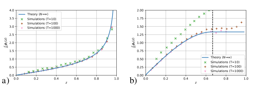
Figure 12: a) First derivative of the rate function $\phi_{d}(z)$ versus $z$, for $d=2$. The continuous blue line corresponds to the exact result in Eq. (172), valid in the limit $N\to\infty$. In this case, no transition occurs. b) First derivative of the rate function $\phi_{d}(z)$ versus $z$, for $d=6$. The continuous blue line corresponds to the exact result in Eq. (174). The vertical dashed line signals the critical point $z_{c}$ at which the phase transition occurs. For $z>z_{c}$, the rate function $\phi_{d}(z)$ becomes exactly linear in $z$. In both panels, the symbols are the results of numerical simulations obtained at finite $N$, as described in Section VII.

We now focus on the large-deviation regime, where $X\sim T$. Some of the results of this section have already been derived in PTV2020 , where the authors compute the rate function of the position of a discrete-time persistent random walk and then take the continuous-time limit to study the RTP. Here, we first present a different and more general technique to compute the rate function for an RTP in $d$ dimensions. Note that our technique can be easily generalized to more complicated RTP models, e.g., with random velocities. Then, we interpret these results in light of the new findings, presented in the previous sections, and we characterize the nature of the phase transition.

It is useful to introduce the scaled variable $z=X/T$. Note that, since $|X|$ cannot exceed the value $T$, corresponding to a straight $x$-direction run with no tumbling, we have $|z|\leq 1$. From Eq. (158), we obtain

$$Z(X=zT,T)\simeq\frac{1}{2\pi i}\int_{\Gamma}dq\,{}_{2}F_{1}\left(\frac{1}{2},1,\frac{d}{2},q^{2}\right)\exp\left[-TS_{d}(q,z)\right]\,,$$ (162)

where

$$S_{d}(q,z)=1-(1+qz)\,{}_{2}F_{1}\left(\frac{1}{2},1,\frac{d}{2},q^{2}\right)\,.$$ (163)

First, we try to compute the integral in Eq. (162) by saddle point approximation. Note that the function ${}_{2}F_{1}\left(\frac{1}{2},1,\frac{d}{2},q^{2}\right)$ has two branch cuts in the complex-$q$ plane, for real $q$ and $|q|>1$. Thus, we need to solve the following saddle point equation

$$z=g_{d}(q)\,$$ (164)

for $|q|<1$, where

$$g_{d}(q)=-\frac{(2q/d)~{}{}_{2}F_{1}\left(3/2,2,1+d/2,q^{2}\right)}{(2q^{2}/d)~{}{}_{2}F_{1}\left(3/2,2,1+d/2,q^{2}\right)+{}_{2}F_{1}\left(1/2,1,d/2,q^{2}\right)}\,.$$ (165)

For any $d$, $g_{d}(q)$ is a decreasing odd function of $q$. We also notice that its maximum value is reached at $q=-1$. To compute this value $g_{d}(-1)$, we use the following asymptotic expansion for the ordinary hypergeometric function Gradshteyn_book

$${}_{2}F_{1}(\alpha,\beta,\gamma,q)\simeq\ \begin{cases}\frac{\Gamma(\gamma)\Gamma(\gamma-\alpha-\beta)}{\Gamma(\gamma-\alpha)\Gamma(\gamma-\beta)}&\text{for }\gamma>\alpha+\beta,\\ \\ \frac{\Gamma(\alpha+\beta)}{\Gamma(\alpha)\Gamma(\beta)}\log\left(\frac{1}{1-q}\right)&\text{for }\gamma=\alpha+\beta,\\ \\ \frac{\Gamma(\gamma)\Gamma(\alpha+\beta-\gamma)}{\Gamma(\alpha)\Gamma(\beta)}(1-q)^{\gamma-\alpha-\beta}&\text{for }\gamma<\alpha+\beta\,,\end{cases}$$ (166)

and we obtain

$$g_{d}(-1)=\ \begin{cases}1&\text{for }d\leq 5,\\ \\ 2/(d-3)<1&\text{for }d>5,\\ \end{cases}$$ (167)

Thus, recalling that $|z|\leq 1$ and focusing on the case $z>0$, for $d\leq 5$ the condition in Eq. (164) is always satisfied for some value $q^{*}(z)>-1$. Thus, for $d<5$ we find that

$$Z(X,T)\sim\exp\left[-T\phi_{d}\left(z=\frac{X}{T}\right)\right]\,,$$ (168)

where

$$\phi_{d}(z)=S_{d}(q^{*}(z),z)\,,$$ (169)

$S_{d}(q,z)$ is given in Eq. (163) and $q^{*}(z)$ is the unique solution of Eq. (164). On the other hand, for $d>5$, the saddle point equation (164) admits a solution only up to some critical value $z=z_{c}=2/(d-3)$, where the condensation transition occurs. For $z>z_{c}$, Eq. (164) has no real solution and the maximum of $S_{d}(q,z)$ is reached at $q=-1$, independently of $z$ and $\phi_{d}(z)=S_{d}(-1,z)$. Thus, for $d>5$ we find that the large-deviation form in Eq. (168) is still valid, with

$$\phi_{d}(z)=\begin{cases}S_{d}(q^{*}(z),z)&\text{for }z<z_{c},\\ \\ -\frac{1}{d-3}+\frac{d-2}{d-3}z&\text{for }z>z_{c}\,,\end{cases}$$ (170)

where $S_{d}(q,z)$ is given in Eq. (163) and $q^{*}(z)$ is the unique solution of Eq. (164). Notably, for $d>5$, the rate function $\phi_{d}(z)$ is non-analytic at $z=z_{c}$. This indicates the presence of the condensation phase-transition. Comparing this result with the one obtained for the fixed-$N$ ensemble, we find that the criterion for condensation is the same for the two models. Indeed, recalling that we are considering $\alpha=0$, here we observe condensation for $\nu=(d-1)/2>2$, exactly as for the fixed-$N$ case.

In the special cases $d=1,2,4,6$, the expression of $\phi_{d}(z)$ becomes simple and is given by

$$\phi_{1}(z) = \frac{1-\sqrt{1-z^{2}}}{2}\,$$ (171)

$$\phi_{2}(z) = 1-\sqrt{1-z^{2}}\,$$ (172)

$$\phi_{4}(z) = z^{2}\,,$$ (173)

$$\phi_{6}(z) = \begin{cases}\frac{3}{2}z^{2}-\frac{9}{16}z^{4}&\text{for }|z|<z_{c},\\ \\ \frac{4}{3}z-\frac{1}{3}&\text{for }|z|>z_{c}\,.\end{cases}$$ (174)

These results for $\phi_{d}(z)$ match with the ones derived in Ref. PTV2020 . The result in Eq. (172), valid for $d=2$, had already been obtained in SBS20 solving the Fokker-Plank equation associated to the system. The rate function of the position distribution of a fixed-$T$ RTP has also been derived in dimension $d=1$ in the presence of a constant drift DM12 .

Note that here we have provided explicit results for the rate function for a specific velocity distribution, namely, when the direction is chosen isotropically and the speed $v=v_{0}$ is a constant. In fact, this rate function, when it exists, can be derived for generic velocity distribution $P(\vec{v})$, as shown in Appendix E.

VI.3 Order of the transition

We now investigate, for $d>5$, the order of the phase transition. Just below the transition, i.e. in the limit $z\to z_{c}$, we expect the solution $q^{*}(z)$ of the saddle point equation (164) to be close to $-1$. Thus, we expand $S_{d}(q,z)$ in Eq. (163) with $q=-1+s$ for small $s$. In the case $5<d<7$, using the asymptotic behavior of the hypergeometric function close to unit value buhring , we find

$$S_{d}(q=-1+s,z)\simeq 1+\frac{d-2}{d-3}(1-z)+\frac{d-2}{d-5}\left(\frac{2}{d-3}-z\right)s-\frac{1}{\sqrt{\pi}}2^{(d-3)/2}\Gamma\left(\frac{d}{2}\right)\Gamma\left(-\frac{d-3}{2}\right)(1-z)s^{(d-3)/2}\,.$$ (175)

Minimizing this expression with respect to $s$ and then expanding for $z\to z_{c}=2/(d-3)$, we obtain

$$\phi_{d}(z)\simeq-\frac{1}{d-3}+\frac{d-2}{d-3}z+c_{d}~{}(z_{c}-z)^{(d-3)/(d-5)}\,,$$ (176)

where $c_{d}$ is a $d$-dependent constant. Comparing this result with the expression for $\phi_{d}(z)$ in the case $z>z_{c}$ in Eq. (170), we conclude that, in this case, the phase transition is of order

$$n=\left\lceil\frac{d-3}{d-5}\right\rceil\,.$$ (177)

On the other hand, in the case $d>7$, the function $S_{d}(q,z)$ can be expanded as

$$S_{d}(q=-1+s,z)\simeq 1+\frac{d-2}{d-3}(1-z)+\frac{d-2}{d-5}\left(\frac{2}{d-3}-z\right)s+\frac{(d-2)\left[3z(d-3)-d-5\right]}{(d-7)(d-5)(d-3)}s^{2}\,.$$ (178)

Minimizing this expression with respect to $s$ and then expanding for $z\to z_{c}$, we obtain

$$\phi_{d}(z)\simeq-\frac{1}{d-3}+\frac{d-2}{d-3}z+\frac{(d-7)(d-3)(d-2)}{4(d-5)(d-1)}(z-z_{c})^{2}\,.$$ (179)

Thus, in this case the order of the transition is $n=2$. Comparing these results with those of Section IV, we notice that the order of the phase transition at given $d$ is the same for the fixed-$N$ and fixed-$T$ ensembles. In Section V, we have shown that the order of the phase transition in the fixed-$T$ ensemble is related to the nature of the condensate itself. In particular, for $5<d<7$, we expect the condensate to have an anomalous shape, with anomalous fluctuations of order $T^{2/(d-3)}$. On the other hand, for $d>7$ the transition becomes of order two and, in analogy with what we observe for the fixed-$N$ ensemble, we expect the condensate to have a Gaussian shape, with fluctuations of order $\sqrt{T}$.

VI.4 Asymptotics of $\phi_{d}(z)$

Here, we investigate the asymptotic behavior of $\phi_{d}(z)$. Let us first consider, for generic $d$, the limit $z\to 0$. In a small region around $z=0$ the rate function $\phi_{d}(z)$ is always given by

$$\phi_{d}(z)=S_{d}(q^{*}(z),z)\,,$$ (180)

where $S_{d}(q,z)$ is given in Eq. (163) and $q^{*}(z)$ is the unique solution of Eq. (164). It is easy to check that for small $z$, $q^{*}(z)$ is also small. Thus, expanding the right-hand side of Eq. (164) for small $q$, we obtain

$$z\simeq-\frac{2}{d}q\,.$$ (181)

Therefore, we find that, at leading order, $q^{*}(z)=-(d/2)z$. Plugging this value into the expression of $S(q,z)$, given in Eq. (163), and expanding for small $z$, we find that

$$\phi_{d}(z)\simeq\frac{d}{4}z^{2}\,.$$ (182)

Plugging this expansion into the expression for $Z(X,T)$ in Eq. (168), we find that, for small $z=X/T$,

$$Z(X,T)\sim\exp\left[-\frac{~{}d}{4T}X^{2}\right]\,.$$ (183)

Thus, the small-$z$ behavior of the rate function $\phi_{d}(z)$ matches smoothly to the typical Gaussian behavior (see Eq. (160)).

Next, we consider the limit $z\to 1$. For $d>5$, we already know from Eq. (170) that, in the limit $z\to 1$, one has

$$\phi_{d}(z)=1+\frac{d-2}{d-3}(z-1)\,.$$ (184)

On the other hand, for $d<5$, the rate function $\phi_{d}(z)$ is given in Eq. (169). Thus, we have to solve Eq. (164) for $z\to 1$. From Eq. (167) we know that $g_{d}(q=-1)=1$, for $d<5$. Thus, we expect the solution $q^{*}(z)$ of Eq. (164) to be of the type $q^{*}(z)=-1+s$ with $s$ small. It is useful to consider the cases $1<d<3$ and $3<d<5$ separately.

In the case $1<d<3$, we plug $q^{*}(z)=-1+s$ in the condition in Eq. (164). Expanding for small $s$ (using Eq. (166)), we obtain

$$z\simeq 1-\frac{d-1}{3-d}s\,,$$ (185)

which yields

$$q^{*}(z)\simeq-1+\frac{3-d}{d-1}(1-z)\,.$$ (186)

Plugging this expression for $q^{*}(z)$ in Eq. (169) and expanding for $z\to 1$ from below, we obtain

$$\phi_{d}(z)\simeq 1-\frac{1}{\sqrt{\pi}}\Gamma\left(\frac{d}{2}\right)\Gamma\left(\frac{3-d}{2}\right)\frac{2}{d-1}\left(2\frac{3-d}{d-1}\right)^{(d-3)/2}~{}(1-z)^{(d-1)/2}\,.$$ (187)

We now consider the case $3<d<5$. Plugging $q^{*}(z)=-1+s$ into Eq. (164) and expanding for small $s$, we find

$$z\simeq 1-\sqrt{\pi}\,\frac{d(d-2)}{4(d-3)}\,\frac{1}{\Gamma\left(1+\frac{d}{2}\right)\Gamma\left(\frac{5-d}{2}\right)}2^{(5-d)/2}s^{(5-d)/2}\,,$$ (188)

which implies

$$1+q^{*}(z)\sim(1-z)^{2/(5-d)}\,.$$ (189)

Plugging this value in Eq. (169) and expanding for $z\to 1$, we obtain

$$\phi_{d}(z)\simeq 1-\frac{d-2}{d-3}~{}(1-z)\,.$$ (190)

To summarize, we have shown that, in the limit $z\to 1$,

$$\phi_{d}(z)=\begin{cases}1-\tilde{c}_{d}~{}(1-z)^{(d-1)/2}+o((1-z)^{(d-1)/2})&~{}~{}~{}~{}~{}\text{for }1<d<3\,,\\ \\ 1-\frac{d-2}{d-3}~{}(1-z)+o((1-z))&~{}~{}~{}~{}~{}\text{for }3<d<5\,,\\ \\ 1-\frac{d-2}{d-3}~{}(1-z)&~{}~{}~{}~{}~{}\text{for }d>5\,,\\ \\ \end{cases}$$ (191)

where $\tilde{c}_{d}$ is a $d$-dependent constant. Thus, for $d<3$, $\phi_{d}(z)$ approaches the limit value $1$, for $z\to 1$, with an exponent $(d-1)/2$ which depends continuously on $d$. For $3<d<5$, the rate function $\phi_{d}(z)$ becomes locally linear for $z\to 1$ and for $d>5$ one has a full region $z_{c}<z<1$ where $\phi_{d}(z)$ is exactly linear.

VII Numerical simulations

In this section we describe the numerical techniques that we have used to verify our theoretical results for the rate function $\psi_{d,\alpha}(z)$, which is defined as

$$\psi_{d,\alpha}(z)=-\lim_{N\to\infty}\frac{\log\left[Z(X=zN,N)\right]}{N}\,,$$ (192)

where $Z(X,N)$ is the distribution of the total $x$-component displacement $X$ after $N$ runs. Let us first recall that, in order to probe the typical Gaussian regime $X\sim\sqrt{N}$, one can use direct sampling. Indeed, a single $x$-direction displacement $x$ can be written as

$$x=v\,\tau\,u\,\,,$$ (193)

where $v>0$ is the speed of the RTP, with distribution $W(v)$, $\tau>0$ is the running time, exponentially distributed with fixed rate $\gamma=1$ and $-1<u<1$ is the $x$-component of the $d$-dimensional unit vector that represents the direction of the RTP. Since this direction is uniformly distributed in space, one can show that $u$ is distributed according to $f_{d}(u)$, given in Eq. (6) MLDM20 ; MLDM20a . Thus, for each of the $N$ running phases, one can generate, by standard sampling techniques, three random number $v_{i}$, $\tau_{i}$ and $u_{i}$ and then one can obtain the $x$-component displacement $x_{i}$ by multiplying these variables. Finally, one can obtain $X$ using the definition

$$X=\sum_{i=1}^{N}x_{i}\,.$$ (194)

This simple and direct procedure is useful to probe the typical regime $X\sim\sqrt{N}$. However, it is unfeasible to adopt such a strategy to compute numerically the large-deviation tails of $Z(X,N)$. For instance, extracting $10^{6}$ samples, one is only able to access events with probabilities of the order $10^{-6}$ or higher. How can one simulate events that happen with very small probability, say of order $10^{-100}$?

In order to compute numerically the large-deviation tails of the PDF $Z(X,N)$ we adopt a technique based on a constrained Markov Chain Monte Carlo (MCMC) algorithm, similar to the one proposed in GM2019 ; NMV10 ; NMV11 . The configuration $\mathcal{C}$ of our system is specified by the set of numbers $\mathcal{C}=\{(v_{1},\tau_{1},u_{1})\,,\ldots\,,(v_{N},\tau_{N},u_{N})\}$ and we are interested in the rate function of

$$X(\mathcal{C})=\sum_{i=1}^{N}v_{i}\tau_{i}u_{i}\,$$ (195)

in the large deviation regime where $X(\mathcal{C})\sim O(N)$. With this goal in mind, we implement a MCMC dynamics in the space of RTP configurations. Let us remark that the MCMC dynamics is defined in configuration space and has nothing to do with the real RTP dynamics. Since we are interested in configurations that correspond to a very large $X(\mathcal{C})$, we impose the constraint $X(\mathcal{C})>X^{*}$, where $X^{*}$ is some fixed $O(N)$ parameter. We choose an initial condition $\mathcal{C}_{0}$ that satisfies the constraint and then we evolve the system using the Metropolis rule. In other words, assuming that at a given step the current configuration is $\mathcal{C}=\{(v_{1},\tau_{1},u_{1})\,,\ldots\,,(v_{N},\tau_{N},u_{N})\}$, we choose one of the running phases $i$ at random and we propose the move $(v_{i},\tau_{i},u_{i})\to({v_{i}}^{\rm new},{\tau_{i}}^{\rm new},u_{i}^{\rm new})$, where

$${v_{i}}^{\rm new}=v_{i}+\delta v\,,$$ (196)

$${\tau_{i}}^{\rm new}=\tau_{i}+\delta\tau\,,$$ (197)

$${u_{i}}^{\rm new}=u_{i}+\delta u\,,$$

where $\delta v$, $\delta\tau$, and $\delta u$ are drawn from a uniform distribution. The new configuration is then simply

$$\mathcal{C}^{\rm new}=\{(v_{1},\tau_{1},u_{1})\,,\ldots\,,({v_{i-1}},{\tau_{i-1}},u_{i-1})\,,({v_{i}}^{\rm new},{\tau_{i}}^{\rm new},u_{i}^{\rm new})\,,\,,({v_{i+1}},{\tau_{i+1}},u_{i+1})\,,\ldots\,,(v_{N},\tau_{N},u_{N})\}$$ (198)

If $\mathcal{C}^{\rm new}$ does not satisfy the constraint $X(\mathcal{C}^{\rm new})>X^{*}$, then the move is immediately rejected. If instead $X(\mathcal{C}^{\rm new})>X^{*}$, the move is accepted with probability

$$p_{\rm acc}=\min\left[1,\frac{e^{-\tau_{i}^{\rm new}}~{}W(v_{i}^{\rm new})f_{d}(u_{i}^{\rm new})}{e^{-\tau_{i}}~{}W(v_{i})f_{d}(u_{i})}\right]\,,$$ (199)

and rejected otherwise. This particular choice of $p_{\rm acc}$, which correspond to the Metropolis-Hastings algorithm, guarantees that the RTP configurations are sampled with the right statistical weight. If the move is accepted we update the current position $\mathcal{C}\to\mathcal{C}^{\rm new}$. Initially, we let the system evolve for $10^{7}$ sweeps (by sweep we denote $N$ move proposals), in order to forget the initial condition. We measure $X(\mathcal{C})$ every $10^{2}$ sweeps, to avoid sample correlations.

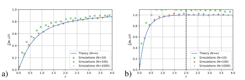
Figure 13: a) First derivative of the rate function $\psi_{d,\alpha}(z)$ versus $z$, for $d=2$ and $\alpha=0$. The continuous blue line corresponds to the exact result in Eq. (56), valid in the limit $N\to\infty$. For this choice of the parameters $d$ and $\alpha$, no transition occurs. b) First derivative of the rate function $\psi_{d,\alpha}(z)$ versus $z$, for $d=6$ and $\alpha=0$. The continuous blue line corresponds to the exact result in Eq. (59). The vertical dashed line signals the critical point $z_{c}$ at which the phase transition occurs. In both panels, the symbols are the results of numerical simulations obtained at finite $N$, as described in Section VII.

With this procedure, we can build an histogram which approximates the PDF $P(X,N|X>X^{*})$ of $X$, conditioned on $X>X^{*}$. This quantity can be written as, for $X>X^{*}$,

$$P(X,N|X>X^{*})=\frac{P(X,N)}{P(X>X^{*})}\,.$$ (200)

Taking the natural logarithm of both sides and using the notation $Z(X,N)=P(X,N)$, we find

$$\log\left[P(X,N|X>X^{*})\right]=\log\left[Z(X,N)\right]-\log\left[P(X>X^{*})\right]\,.$$ (201)

Note that the last term is independent of $X$. Using the definition of $\psi_{d,\alpha}(z)$, given in Eq. (192), we find, for large $N$,

$$\log\left[P(X,N|X>X^{*})\right]=-N\psi_{d,\alpha}\left(\frac{X}{N}\right)-\log\left[P(X>X^{*})\right]\,,$$ (202)

Finally, taking a derivative with respect to $X$ on both sides, we get

$$\psi_{d,\alpha}^{\prime}\left(\frac{X}{N}\right)=-\frac{d}{dX}\log\left[P(X,N|X>X^{*})\right]\,,$$ (203)

where $\psi_{d,\alpha}^{\prime}(z)=\frac{d}{dz}\psi_{d,\alpha}(z)$. Thus, we are able to compute numerically the first derivative of the rate function. Then, one can obtain $\psi_{d,\alpha}(z)$ via numerical integration. Note however that, with the method described above, one can only probe a small region $(X^{*},X^{*}+\Delta)$, where $\Delta>0$ is a small number compared to $X^{*}$. Therefore, one has to use several values of $X^{*}$ in order to sample the large-deviation regime. In our case, we used $20$ different values of $X^{*}$. Our numerical estimate of $\frac{d}{dz}\psi_{d,\alpha}(z)$ is shown in Fig. 13 for $\alpha=0$, $d=2,6$ and for different values of $N$. In the case $N=10^{4}$, the numerical curves are in excellent agreement with the theory, both in the fluid and in the condensed phases. Integrating $\frac{d}{dz}\psi_{d,\alpha}(z)$ numerically, we also compute $\psi_{d,\alpha}(z)$, which is shown in Fig. 9 and is in excellent agreement with the theory. Similarly, one can also compute the PDF $Z(X,N)$, which is shown, for $d=2$ and $\alpha=0$, in Fig. 14 with precision smaller than $10^{-100}$.

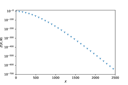
Figure 14: Numerical curve of the PDF $Z(X,N)$ as a function of $X$, for $d=2$, $\alpha=0$ and $N=1000$, obtained with the constrained Markov Chain Monte Carlo algorithm described in the text.

In the case of the fixed-$T$ ensemble, a similar algorithm can be applied. The only complication is that the number of running phases is not fixed anymore. Therefore, it might happen that, proposing a move, the total simulation time becomes shorter than $T$. In such a case, we simply add a new running phase at the end of the trajectory. In this way, one obtains the first derivative of $\phi_{d}(z)$, which is shown in Fig. 12 for $d=2,6$ and for different values of $N$. Note that for the fixed-$T$ ensemble one has $z<1$, since the maximal distance that one can travel in a time $T$ is $v_{0}T$. For this reason, sampling the region close to $z=1$ becomes increasingly complicated. Nevertheless, in Fig. 12, we observe a good agreement between the numerics and the theoretical curve.

With the technique described above, one can also sample the marginal probability distribution $p(x|X)$ of a single-run displacement. This can be achieved by using the MCMC algorithm described above, keeping $X^{*}$ fixed. During the Monte Carlo dynamics, one has access to the full configuration $\mathcal{C}$ of the RTP. Thus, one can sample the single-run displacement $x$, for instance choosing $x=x_{1}$. To be precise, since $X$ has to satisfy the constraint $X>X^{*}$ (and not $X=X^{*}$), in this way one would compute the marginal probability $p(x|X>X^{*})$, conditioned on the event $X>X^{*}$. However, since in practice the system is always in a small region $(X^{*},X^{*}+\Delta)$, one has that $p(x|X>X^{*})$ is a good approximation of $p(x|X^{*})$ (see Fig. 3).

Finally, let us mention that a similar method, based on an exponentially biased MCMC algorithm, has been proven useful to simulate large deviations of the RTP model DMS21 ; HMS20 . However, to the best of our knowledge, such techniques cannot be used to simulate the RTP model in the condensed phase.

VIII Conclusions

In this paper, we have investigated the late-time position of a single RTP in $d$ dimensions, with velocity distribution $W(v)$ and tumbling rate $\gamma$. First, we have focused on the fixed-$N$ ensemble, i.e., we have considered the number $N$ of running phases to be fixed. We have shown that due to the isotropy of the process, it is sufficient to study the distribution $Z(X,N)$ of the displacement of the particle in the $x$-component after $N$ running phases. We have observed that, even if in the typical regime where $X\sim\sqrt{N}$ the PDF $Z(X,N)$ has a Gaussian shape, its large-deviation tails still carry the signatures of the active nature of the process. Moreover, we have shown that for several choices of $d$ and $W(v)$, the system undergoes a dynamical condensation transition in the large-deviation regime. This transition is signaled by a singularity of the rate function of $Z(X,N)$. Below the transition, all running phases contribute to the total displacement $X$ by roughly the same amount. On the other hand, above some critical value $X=X_{c}$, a condensate emerges in the form of a single run which dominates the RTP trajectory. Using a grand-canonical argument, we have identified a precise criterion for condensation.

In the special case $W(v)=\alpha(1-v)^{\alpha-1}$, we have exactly computed the rate function $\psi_{d,\alpha}(z)$, where $z=X/N$. We have shown that condensation happens only if $\nu=(d+2\alpha-1)/2>2$. In particular, for $\nu>3$, we have observed that $\psi_{d,\alpha}(z)$ has a second-order singularity at some critical value $z_{c}$, which we have computed exactly, while for $2<\nu<3$ the order of the transition depends continuously on $\nu$. Moreover, we have investigated the precise nature of the condensate, studying the marginal probability of a single-run displacement. For $\nu>3$, we have observed that the condensate size has Gaussian fluctuations of order $\sqrt{N}$. On the other hand, for $2<\nu<3$, we have shown that the condensate has an anomalous shape, with large fluctuations of order $N^{1/(\nu-1)}$. We have also extended our results to the fixed-$T$ ensemble, where the total duration $T$ of the trajectory is fixed. In the case of fixed velocity ($\alpha=0$), we have computed the rate function of the total displacement $X$ of the particle for arbitrary $d$. We have observed that an analogous condensation transition occurs also for this model above some critical value $X_{c}$ of $X$. Moreover, we have employed a constrained Markov chain Monte Carlo technique to verify our large-deviation result, probing events with probability smaller than $10^{-100}$. Our numerical simulations are in excellent agreement with our theoretical results.

In this paper, we have shown that condensation transitions are a general feature of the RTP model. In future works, it would be interesting to investigate other RTP models that satisfy the condensation criterion. We have shown that a second-order transition is linked to a normal condensate, while a higher-order transition corresponds to an anomalous condensate. Therefore, it would be relevant to investigate what happens in models that display a first-order condensation transition, see e.g. GM2019 .

Another interesting open problem is related to the criterion for condensation. The argument we have presented is based on a grand canonical description of the system, which fails if the single-run distribution $p(x)$ decays slower than any exponential. In this case, we have conjectured that a condensation transition will occur if $p(x)$ decays faster than $1/|x|^{3}$ for large $|x|$. It would be interesting to prove this conjecture.

Appendix A Relation between $P(\vec{R},N)$ and $Z(X,N)$

In this appendix, we derive the relation in Eq. (1) between the PDF $P(\vec{R},N)$ of the position $\vec{R}$ of the RTP after $N$ steps and the distribution $Z(X,N)$ of the $x$-component $X$ of $\vec{R}$. Moreover, we show that $Z(X,N)$ and $P(\vec{R},N)$ share the same rate function $\psi(z)$ in the large-deviation regime where $X$ and $R=|\vec{R}|$ scale linearly with $N$. As a consequence of the isotropy of the process, the PDF $P(\vec{R},N)$ depends only on the magnitude $R$ of $\vec{R}$ and not on its orientation. In other words, the orientation of $\vec{R}$ is distributed uniformly at random. Given a vector $\vec{R}$ with fixed norm $R$ and random orientation, it is possible to show that the PDF of the $x$-component $X$ of $\vec{R}$ is (see Appendix A of MLDM20 )

$$P(X|R)=\frac{1}{R}f_{d}\left(\frac{X}{R}\right)\,,$$ (204)

where the function $f_{d}(z)$ can be computed for any $d$ and is given in Eq. (6). Thus, the PDF of $X$ can be written as

$$Z(X,N)=\int_{\mathbb{R}^{d}}d\vec{R}~{}\frac{1}{R}f_{d}\left(\frac{X}{R}\right)P(R,N)\,,$$ (205)

where we integrate over all possible values of $\vec{R}$, weighted by the PDF $P(\vec{R},N)=P(R,N)$. This is precisely the relation given in Eq. (1).

We now want to show that in the large-deviation regime where $|X|\sim O(N)$ and $R\sim O(N)$, $Z(X,N)$ and $P(\vec{R},N)$ share the same rate function $\psi(z)$. We can perform the integral in Eq. (205) in the radial coordinate and we obtain

$$Z(X,N)=\frac{2\pi^{d/2}}{\Gamma(d/2)}\int_{0}^{\infty}dR~{}R^{d-2}f_{d}\left(\frac{X}{R}\right)P(R,N)\,.$$ (206)

Using the expression of $f_{d}(z)$, given in Eq. (6), we obtain

$$Z(X,N)=\frac{2\pi^{(d-1)/2}}{\Gamma((d-1)/2)}\int_{|X|}^{\infty}dR~{}R^{d-2}\left(1-\frac{X^{2}}{R^{2}}\right)^{(d-3)/2}P(R,N)\,,$$ (207)

and making the change of variable $R\to u=R/X$, we obtain

$$Z(X,N)=\frac{2\pi^{(d-1)/2}}{\Gamma((d-1)/2)}|X|^{d-1}\int_{1}^{\infty}du~{}u^{d-2}\left(1-u^{-2}\right)^{(d-3)/2}P(R=u|X|,N)\,.$$ (208)

Let us now focus on the regime where $X\sim O(N)$. Plugging the scaled variable $z=X/N$ in Eq. (208), we find

$$Z(X=zN,N)=\frac{2\pi^{(d-1)/2}}{\Gamma((d-1)/2)}|zN|^{d-1}\int_{1}^{\infty}du~{}u^{d-2}\left(1-u^{-2}\right)^{(d-3)/2}P(R=u|z|N,N)\,.$$ (209)

In the large deviation regime where $R\sim O(N)$, we expect $P(R,N)\sim\exp\left[-N\psi(R/N)\right]$, where $\psi(z)$ is the rate function associated to $P(R,N)$. Plugging this expression in Eq. (209), we find

$$Z(X=zN,N)\sim\int_{1}^{\infty}du~{}u^{d-2}\left(1-u^{-2}\right)^{(d-3)/2}e^{-N\psi(u|z|)}\,.$$ (210)

In the limit of large $N$, this integral is dominated by values close to the lower limit $u=1$. Thus, we obtain

$$Z(X=zN,N)\sim e^{-N\psi(|z|)}\,,$$ (211)

which can be written as

$$Z(X,N)\sim e^{-N\psi(|X|/N)}\,.$$ (212)

Therefore, $Z(X,N)$ and $P(\vec{R},N)$ have the same rate function $\psi(z)$.

Appendix B Distribution of the $x$-direction displacements

In this appendix, we want to compute the distribution of the $x$-direction displacements $x_{1}\,,\ldots\,,x_{N}$ of the RTP associated to the $N$ running phases. For $1\leq i\leq N$, $x_{i}$ is the $x$-component of the $d$-dimensional vector $\vec{\ell}_{i}$. These vectors $\vec{\ell}_{i}$ are i.i.d. random variables, their direction is drawn uniformly at random and their magnitude is given by $\ell_{i}=v_{i}\,\tau_{i}$, where $v_{i}>0$ is drawn from the speed distribution $W(v)$ and $\tau_{i}$ is an exponential random variable with rate $\gamma$. Thus, the distribution of the magnitude $\ell$ of one of these displacement vectors is

$$P(\ell)=\int_{0}^{\infty}d\tau\,\int_{0}^{\infty}dv~{}W(v)~{}\gamma e^{-\gamma\tau}\delta\left(\ell-v\tau\right)\,.$$ (213)

Performing the integral over $\tau$, we get

$$P(\ell)=\int_{0}^{\infty}dv~{}\frac{1}{v}W(v)~{}\gamma e^{-\gamma(\ell/v)}\,.$$ (214)

One can then show that the distribution of the $x$-component of a $d$-dimensional vector $\vec{l}$ with fixed norm and uniformly distributed direction is given by

$$p(x|l)=\frac{1}{l}f_{d}\left(\frac{x}{l}\right)\,,$$ (215)

where

$$f_{d}(z)=\frac{\Gamma\left(d/2\right)}{\sqrt{\pi}\Gamma\left((d-1)/2\right)}(1-z^{2})^{(d-3)/2}\theta(1-|z|)\,,$$ (216)

$\Gamma(y)$ is the Gamma function and $\theta(y)$ is the Heaviside theta function. For a derivation of this result in Eq. (216) see Appendix A of MLDM20 . Thus, the distribution $p(x)$ of the displacement $x$ of the particle during a single running phase is given by, using Eqs. (214) and (215),

$$p(x)=\int_{0}^{\infty}dv~{}\frac{1}{v}W(v)\int_{0}^{\infty}d\ell~{}\frac{1}{\ell}f_{d}\left(\frac{x}{\ell}\right)~{}\gamma e^{-\gamma(\ell/v)}\,.$$ (217)

Note that, since $f_{d}(z)$ is symmetric around $z=0$, the PDF $p(x)$ is also symmetric around $x=0$.

Appendix C Large-$|x|$ behavior of $p(x)$

The result in Eq. (217) is valid for any distribution $W(v)$. We now consider the special case where

$$W(v)=\frac{\alpha}{v_{0}}\left(1-\frac{v}{v_{0}}\right)^{\alpha-1}~{}\theta(v)~{}\theta(v_{0}-v)\,.$$ (218)

In particular, we are interested in computing the large-$x$ behavior of $p(x)$. Using the expression for $W(v)$ given in Eq. (218), we find

$$p(x)=\frac{\Gamma\left(d/2\right)}{\sqrt{\pi}\Gamma\left((d-1)/2\right)}\frac{\alpha}{v_{0}}\gamma\int_{x}^{\infty}d\ell~{}\frac{1}{\ell}\left(1-\frac{x^{2}}{\ell^{2}}\right)^{(d-3)/2}\int_{0}^{v_{0}}dv~{}\frac{1}{v}\left(1-\frac{v}{v_{0}}\right)^{\alpha-1}~{}e^{-\gamma\ell/v}\,.$$ (219)

Performing the changes of variable $\ell\to u=x/\ell$ and $v\to w=v/v_{0}$, we find

$$p(x)=\frac{\Gamma\left(d/2\right)}{\sqrt{\pi}\Gamma\left((d-1)/2\right)}\frac{\alpha}{v_{0}}\gamma\int_{0}^{1}du~{}\frac{1}{u}\left(1-u^{2}\right)^{(d-3)/2}\int_{0}^{1}dw~{}\frac{1}{w}\left(1-w\right)^{\alpha-1}~{}e^{-\gamma x/(v_{0}wu)}\,.$$ (220)

It is useful to perform the changes of variable $u\to t=1-u^{2}$ and $w\to s=1-w$, and we obtain

$$p(x)=\frac{1}{2}\frac{\Gamma\left(d/2\right)}{\sqrt{\pi}\Gamma\left((d-1)/2\right)}\frac{\alpha}{v_{0}}\gamma\int_{0}^{1}dt~{}\frac{1}{1-t}t^{(d-3)/2}\int_{0}^{1}ds~{}\frac{1}{1-s}s^{\alpha-1}~{}\exp\left(-\frac{\gamma}{v_{0}}\frac{x}{(1-s)\sqrt{1-t}}\right)\,.$$ (221)

For $x\gg 1$, the integral is dominated by small values of $s$ and $t$, thus, expanding for small $s$ and $t$, we find

$$p(x)\simeq\frac{1}{2}\frac{\Gamma\left(d/2\right)}{\sqrt{\pi}\Gamma\left((d-1)/2\right)}\frac{\alpha}{v_{0}}\gamma e^{-\gamma x/v_{0}}\int_{0}^{1}dt~{}e^{-\gamma xt/(2v_{0})}t^{(d-3)/2}\int_{0}^{1}ds~{}e^{-\gamma xs/v_{0}}s^{\alpha-1}~{}\,.$$ (222)

Computing the integrals, we find

$$p(x)\simeq\frac{\Gamma\left(d/2\right)}{\sqrt{\pi}\Gamma\left((d-1)/2\right)}\frac{\alpha}{v_{0}}\gamma e^{-\gamma x/v_{0}}2^{(d-3)/2}\left(\frac{v_{0}}{\gamma x}\right)^{(d+2\alpha-1)/2}\Gamma\left(\frac{d-1}{2}\right)\Gamma\left(\alpha\right)~{}\,.$$ (223)

Finally, using the symmetry of $p(x)$, we find that for $|x|\gg 1$,

$$p(x)\simeq A_{d,\alpha}\frac{\gamma}{v_{0}}e^{-\gamma|x|/v_{0}}\left(\frac{v_{0}}{\gamma|x|}\right)^{(d+2\alpha-1)/2}~{}\,,$$ (224)

where

$$A_{d,\alpha}=\frac{\Gamma\left(d/2\right)\alpha\Gamma\left(\alpha\right)}{\sqrt{\pi}}2^{(d-3)/2}\,.$$ (225)

Appendix D Range of validity of the Central Limit Theorem

Consider $N$ i.i.d. random variables $\{x_{1},x_{2},\cdots,x_{N}\}$ each drawn from a normalised distribution $p(x)$. The distribution of their sum $X$ can be expressed as

$$Z(X,N)=\int_{-\infty}^{\infty}dx_{1}\,\ldots\int_{-\infty}^{\infty}dx_{N}~{}\left[\prod_{i=1}^{N}p(x_{i})\right]\delta\left(X-\sum_{i=1}^{N}x_{i}\right)\,.$$ (226)

Taking a Fourier transform factorises the $N$-fold integrals

$$\int_{-\infty}^{\infty}Z(X,N)\,e^{i\,k\,X}\,dX=\left[\hat{p}(k)\right]^{N}\,,$$ (227)

where

$$\hat{p}(k)=\int_{-\infty}^{\infty}p(x)\,e^{i\,k\,x}\,dx$$ (228)

is the Fourier transform of $p(x)$. Finally, inverting the Fourier transform in Eq. (227) one gets the integral representation

$$Z(X,N)=\int_{-\infty}^{\infty}\frac{dk}{2\pi}\,e^{-i\,k\,X}\,\left[\hat{p}(k)\right]^{N}\,.$$ (229)

Note that this expression is valid for all $X$ and all $N$ and arbitrary $p(x)$. Motivated by the RTP problem, we focus on $p(x)$’s that are symmetric with a finite second moment $\sigma^{2}$. In this case, the central limit theorem (CLT) is valid for large $N$ which predicts that in the region up to $|X|\sqrt{N}$, the distribution $Z(X,N)$ converges to a Gaussian shape for large $N$

$$Z(X,N)\simeq\frac{1}{\sqrt{2\pi\,\sigma^{2}\,N}}e^{-X^{2}/(2\,\sigma^{2}\,N)}\,.$$ (230)

One may ask whether this Gaussian shape remains valid over a larger range, outside the region $X\sim\sqrt{N}$ of the validity of the CLT.

To answer this question, we start from the integral representation of $Z(X,N)$ in Eq. (229) which can be rewritten as

$$Z(X,N)=\int_{-\infty}^{\infty}\frac{dk}{2\pi}\,e^{-i\,k\,X+N\,\log(\hat{p}(k))}\,.$$ (231)

In order to probe the Gaussian regime where $X\sim\sqrt{N}$, we first set $y=X/\sqrt{N}$. Performing the change of variable $k\to k/\sqrt{N}$ in Eq. (229) gives

$$Z(X,N)=\frac{1}{\sqrt{N}}\int_{-\infty}^{\infty}\frac{dk}{2\pi}\,e^{-i\,k\,y+N\,\log(\hat{p}(k/\sqrt{N}))}\,.$$ (232)

Thus large $N$ limit probes the small $k$ behavior of $\hat{p}(k)$ defined in Eq. (228). We next assume that $\hat{p}(k)$ has the small $k$ expansion

$$\hat{p}(k)\simeq 1-\frac{\sigma^{2}\,k^{2}}{2}+c\,|k|^{\beta}+\cdots$$ (233)

where $2<\beta\leq 4$. Since we assumed $p(x)$ to be normalised to unity, the first term is unity. Moreover, since $p(x)$ is symmetric, there is no linear term in $\hat{p}(k)$ in the small $k$ expansion. The second term is automatic since the variance $\sigma^{2}$ is finite and the third correction term must appear with exponent $\beta>2$. We also assume that $\beta\leq 4$. The prefactor $c$ of $|k|^{\beta}$ is just an unimportant nonzero constant.

Substituting the small $k$ expansion (233) in (232) in the large $N$ limit we get, keeping only leading order terms up to $O(|k|^{\beta})$ (note that $2<\beta\leq 4$),

$$Z(X,N)\simeq\frac{1}{\sqrt{N}}\int_{-\infty}^{\infty}\frac{dk}{2\pi}\,~{}e^{-i\,k\,y-\sigma^{2}k^{2}/2+c\,N^{1-\beta/2}\,|k|^{\beta}}\,,$$ (234)

If $\beta<4$, then the prefactor of the third term inside the exponent is $c$. However, if $\beta=4$, then this prefactor will be slightly modified from $c$ since the expansion of the logarithm will give rise to a term of $O(k^{4})$ also. But in any case, we just need that $c$ is some nonzero constant in Eq. (234). It is possible to check that in the case of the RTP model considered in Section IV, one has $\beta=4$. Since $\beta>2$, the term $cN^{1-\beta/2}\,|k|^{\beta}$ is small for large $N$, and we can expand the exponential as

$$Z(X,N)\simeq\frac{1}{2\pi}\frac{1}{\sqrt{N}}\int_{-\infty}^{\infty}dk~{}e^{-i\,k\,y-\sigma^{2}k^{2}/2}\left(1+c\,N^{1-\beta/2}\,|k|^{\beta}\right)\,.$$ (235)

Performing the first integral gives the leading Gaussian term and rearranging the second term slightly gives

$$Z(X,N)\simeq\frac{1}{\sqrt{2\pi N\sigma^{2}}}e^{-y^{2}/(2\sigma^{2})}\left[1+\sqrt{2\pi\sigma^{2}}cN^{1-\beta/2}\int_{-\infty}^{\infty}dk~{}e^{-(\sigma^{2}/2)(k-iy/\sigma^{2})^{2}}|k|^{\beta}\right]\,.$$ (236)

Performing the change of variable $k\to k+iy/\sigma^{2}$, we obtain

$$Z(X,N)\simeq\frac{1}{\sqrt{2\pi N\sigma^{2}}}e^{-y^{2}/(2\sigma^{2})}\left[1+\sqrt{2\pi\sigma^{2}}cN^{1-\beta/2}\int_{-\infty}^{\infty}dk~{}e^{-(\sigma^{2}/2)k^{2}}|k+iy/\sigma^{2}|^{\beta}\right]\,.$$ (237)

When $y$ is of order one, i.e. when $X\sim O(\sqrt{N})$, the correction term vanishes as $N^{1-\beta/2}$ and we obtain the leading Gaussian term, as predicted by the CLT. On the other hand, for $y\gg 1$, the second integral over $k$ can be approximated to leading order for large $y$ as

$$Z(X,N)\simeq\frac{1}{\sqrt{2\pi N\sigma^{2}}}e^{-y^{2}/(2\sigma^{2})}\left[1+\tilde{c}N^{1-\beta/2}y^{\beta}\right]\,,$$ (238)

where $\tilde{c}$ is just a constant. The correction term can be neglected when $N^{1-\beta/2}y^{\beta}\ll 1$ and therefore the CLT is valid for any $y$ such that $y\ll N^{(\beta-2)/(2\beta)}$. Recalling that $y=X/\sqrt{N}$, we obtain that the CLT is valid up to a wider range than $\sqrt{N}$, namely, up to

$$|X|\ll N^{(\beta-1)/\beta}\,.$$ (239)

For instance, for the RTP model considered in Section IV, we have $\beta=4$ and thus the CLT is valid for $|X|\ll N^{3/4}$.

Appendix E Large deviation for the position distribution in the $x$ direction

In this Appendix we give a formula for the large deviation of the $x$ coordinate in the fixed $T$ ensemble of the RTP, valid for a model with an arbitrary distribution of velocity, using an equivalent but slightly different method as in the text. Let us recall that the displacements $x_{i}$ along the $x$ axis, and the durations $\tau_{i}$ associated to the $i$-th running phase are i.i.d. variables, except for the last run which is incomplete and hence has a different distribution. Their distribution is $P(x,\tau)=p(x|\tau)\gamma e^{-\gamma\tau}$, with $p(x|\tau)=\int d^{d}\vec{v}P(\vec{v})\delta(x-v_{1}\tau)=\langle\delta(x-v_{1}\tau)\rangle$, where $v_{1}=\vec{v}\cdot e_{x}$ denotes the first component of the velocity, and here and below $\langle\cdots\rangle$ denotes an average with respect to the distribution of the velocity $\vec{v}$ (here assumed to be quite general). Thus one can write

$$\hat{p}(q,s)=\int_{-\infty}^{+\infty}dx\int_{0}^{+\infty}d\tau~{}e^{-qx-s\tau}\langle\delta(x-v_{1}\tau)\rangle\gamma e^{-\gamma\tau}=\left\langle\frac{\gamma}{\gamma+s+qv_{1}}\right\rangle\,.$$ (240)

For an isotropic distribution with $|\vec{v}|=v_{0}$ in dimension $d$, the explicit form is given in (153) in the text.

Let us start from Eq. (151) and set $\gamma=1$ for simplicity. Eq. (151) can be written as

$$\int_{0}^{+\infty}dT\int_{-\infty}^{+\infty}dXe^{-sT-qX}Z(X,T)=\frac{\hat{p}(q,s)}{1-\hat{p}(q,s)}\,.$$ (241)

Let us first assume that $Z(X,T)$ admits a large deviation form $Z(X,T)\sim e^{-T\phi_{d}(z=X/T)}$. Inserting this form on the left-hand side of Eq. (241), we get

$$\int_{0}^{+\infty}dT~{}T\int_{-\infty}^{+\infty}dz~{}e^{-sT-qTz-T\phi_{d}(z)}\sim\int_{0}^{+\infty}dT~{}Te^{-sT-T\min_{z\in\mathbb{R}}(qz+\phi_{d}(z))}\,,~{}$$ (242)

where we used a saddle point estimate in the integral over $z=X/T$. This integral becomes divergent when $s$ decreases and reaches

$$s=s(q):=-\min_{z}[qz+\phi_{d}(z)]\,.$$ (243)

Now looking at the right-hand side of Eq. (241) we see that we expect a singularity when $\hat{p}(q,s)=1$. We will surmise that these singularities are the same

$$\hat{p}(q,s)=1\quad\Leftrightarrow\quad s=s(q)\,.$$ (244)

More explicitly the function $s(q)$ is the root $s=s(q)$ of the equation

$$\left\langle\frac{1}{1+s+qv_{1}}\right\rangle=1\quad\Leftrightarrow~{}~{}\left\langle\frac{s+qv_{1}}{1+s+qv_{1}}\right\rangle=0\,.$$ (245)

Once $s(q)$ is known, the inversion of (243) determines the large deviation function

$$\phi_{d}(z)=\max_{q}(-qz-s(q))\,.$$ (246)

These formulae allow to easily determine the small $z$ behavior of the large deviation function as a function of the moments of the random variable $v_{1}$, assuming that they exist. Expanding (245) in powers of $q$ to second order one obtains $\phi_{d}(z)$ to quadratic order

$$s(q)=-\langle v_{1}\rangle q+\langle(v_{1}-\langle v_{1}\rangle)^{2}\rangle q^{2}+O(q^{3})\quad\Rightarrow\quad\phi_{d}(z)=\max_{q}(-qz-s(q))=\frac{(z+\langle v_{1}\rangle)^{2}}{4\langle v_{1}^{2}\rangle}+O(z^{3})$$ (247)

where we have not assumed any symmetry of the distribution of $\vec{v}$. When the distribution of $v_{1}$ is symmetric in $v_{1}\to-v_{1}$, it is convenient to symmetrize (245) and rewrite it as $\langle\frac{s(1+s)-q^{2}v_{1}^{2}}{(1+s)^{2}-q^{2}v_{1}^{2}}\rangle=0$. One obtains using Mathematica $s(q)=c_{2}q^{2}+(c_{4}-2c_{2}^{2})q^{4}+(c_{6}-6c_{2}c_{4}+7c_{2}^{3})q^{6}+O(q^{8})$ and

$$\phi_{d}(z)=\frac{z^{2}}{4c_{2}}-\frac{\left(c_{4}-2c_{2}^{2}\right)z^{4}}{16c_{2}^{4}}+\frac{\left(9c_{2}^{4}-10c_{4}c_{2}^{2}-c_{6}c_{2}+4c_{4}^{2}\right)z^{6}}{64c_{2}^{7}}+O\left(z^{8}\right)\quad,\quad c_{n}:=\langle v_{1}^{n}\rangle\,.$$ (248)

Note that for an isotropic distribution of $\vec{v}$, with $\langle\vec{v}^{2}\rangle=1$, $c_{2}=1/d$ and $\phi_{d}(z)=\frac{d}{4}z^{2}+O(z^{4})$, as in Eq. (182).

The saddle point equation (245) can be conveniently rewritten by performing the change of variable $w=q/(1+s)$ and introducing the function

$$F(w):=\left\langle\frac{1}{1+v_{1}w}\right\rangle\,.$$ (249)

Simple manipulations then lead to $\phi_{d}(z)=\max_{q}(-qz-s(q))=\max_{w}(1-(1+zw)F(w))$. The function $\phi_{d}(z)$ can then be obtained in a parametric form (by eliminating $w$)

$$z=-\frac{F^{\prime}(w)}{F(w)+wF^{\prime}(w)}\quad,\quad\phi_{d}(z)=1-(1+zw)F(w)=1-\frac{F(w)^{2}}{F(w)+wF^{\prime}(w)}$$ (250)

where one can alternatively use the simpler formula $\phi_{d}^{\prime}(z)=-wF(w)$.

For an isotropic distribution of velocities with $|\vec{v}|=1$ in dimension $d$, one has $F(w)={}_{2}F_{1}\left(\frac{1}{2},1;\frac{d}{2};w^{2}\right)$ and one recovers the formula (163), (164) and (165) given in the text (where the variable $w$ is $q$ there). They are valid as long as $|w|<1$, beyond which the saddle point value freezes at $w=\pm 1$, as discussed in the text.

We have assumed so far that the function $F(w)$, defined in Eq. (249), exists. Of course there are some distributions $P(\vec{v})$ for which the average in Eq. (249) may not exist. In fact, for any distribution $P(\vec{v})$ which is nonzero at $v_{1}=-1/w$, the average in Eq. (249) is divergent. An example of this is simply the Gaussian distribution $P(\vec{v})=e^{-{\vec{v}}^{2}/2}/(2\pi)^{d/2}$. Recall that in the main text we have chosen the direction isotropically and taken the speed distribution $W(v)=\alpha(1-v)^{\alpha-1}$, which has a finite support $v\in(0,1)$. In this example the average in Eq. (249) is well defined. In cases where $F(w)$ in Eq. (249) does not exist, it indicates that the distribution does not admit a large-deviation form on a scale $X\sim O(T)$, as assumed. In this case, a condensation may still occur, but at a smaller scale $X\sim T^{\gamma}$ with $1/2<\gamma<1$.

References

- (1) M. E. Cates, Rep. Prog. Phys. 75, 042601 (2012).
- (2) M. C. Marchetti, J. F. Joanny, S. Ramaswamy, T. B. Liverpool, J. Prost, M. Rao, and R. Aditi Simha, Rev. Mod. Phys. 85, 1143 (2013).
- (3) C. Bechinger, R. Di Leonardo, H. Löwen, C. Reichhardt, G. Volpe, and G. Volpe, Rev. Mod. Phys. 88, 045006 (2016).
- (4) S. Ramaswamy, J. Stat. Mech. 054002 (2017).
- (5) É. Fodor and M. C. Marchetti, Physica A 504, 106 (2018).
- (6) L. Walsh, C. G. Wagner, S. Schlossberg, C. Olson, A. Baskaran, and N. Menon, Soft matter, 13, 8964 (2017).
- (7) S. Ramaswamy, Annu. Rev. Condens. Matter Phys. 1, 323 (2010).
- (8) R. Nitzan, R. Voituriez, and N. S. Gov, Phys. Rev. E 99, 022419 (2019).
- (9) H. C. Berg, E. coli in Motion (Springer, 2014).
- (10) J. Tailleur and M. E. Cates, Phys. Rev. Lett. 100, 218103 (2008).
- (11) T. Vicsek, A. Czirók, E. Ben-Jacob, I. Cohen, and O. Shochet, Phys. Rev. Lett. 75, 1226 (1995).
- (12) S. Hubbard, P. Babak, S. T. Sigurdsson, and K. G. Magnússon, Ecological Modelling, 174, 359 (2004).
- (13) T. Vicsek and A. Zafeiris, Phys. Rep. 517, 71 (2012).
- (14) É. Fodor, C. Nardini, M. E. Cates, J. Tailleur, P. Visco, and F. van Wijland, Phys. Rev. Lett 117, 038103 (2016).
- (15) L. L. Bonilla, Phys. Rev. E 100, 022601 (2019).
- (16) F. J. Sevilla, R. F. Rodriguez, and J. R. Gomez-Solano, Phys. Rev. E 100, 032123 (2019).
- (17) E. Woillez, Y. Kafri and V. Lecomte, J. Stat. Mech. 063204 (2020).
- (18) P. Pietzonka, K. Kleinbeck, and U. Seifert, New J. Phys. 18, 052001 (2016).
- (19) C. Kurzthaler, C. Devailly, J. Arlt, T. Franosch, W. C. K. Poon, V. A. Martinez, and A. T. Brown, Phys. Rev. Lett. 121, 078001 (2018).
- (20) U. Basu, S. N. Majumdar, A. Rosso, and G. Schehr, Phys. Rev. E, 98, 062121 (2018).
- (21) U. Basu, S. N. Majumdar, A. Rosso, and G. Schehr, Phys. Rev. E, 100, 062116 (2019).
- (22) T. GrandPre, and D. T. Limmer, Phys. Rev. E 98, 060601(R) (2018).
- (23) A. Shee, A. Dhar, and D. Chaudhuri, Soft Matter, 16, 4776 (2020).
- (24) S. N. Majumdar and B. Meerson, Phys. Rev. E 102, 022113 (2020).
- (25) I. Santra, U. Basu, and S. Sabhapandit, preprint arXiv:2101.11327 (2021).
- (26) M. Kac, Rocky Mountain J. Math. 4, 497 (1974).
- (27) W. Stadje, J. Stat. Phys. 46, 207 (1987).
- (28) E. Orsingher, Stoch. Process. Their Appl. 34, 49 (1990).
- (29) G. H. Weiss, Physica A 311, 381 (2002).
- (30) P. Hänggi and P. Jung, Adv. Chem. Phys. 89, 239 (1995).
- (31) J. Masoliver and K. Lindenberg, Eur. Phys. J. B 90, 1 (2017).
- (32) M. E. Cates and J. Tailleur, Annu. Rev. Condens. Matter Phys. 6, 219 (2015).
- (33) A. P. Solon, Y. Fily, A. Baskaran, M. E. Cates, Y. Kafri, M. Kardar, and J. Tailleur, Nature Phys. 11, 673 (2015).
- (34) A. B. Slowman, M. R. Evans, and R. A. Blythe, Phys. Rev. Lett. 116, 218101 (2016).
- (35) K. Martens, L. Angelani, R. Di Leonardo, and L. Bocquet, Eur. Phys. J. E 35, 84 (2012).
- (36) L. Angelani, J. Phys. A: Math. Theor. 48, 495003 (2015).
- (37) K. Malakar, V. Jemseena, A. Kundu, K. V. Kumar, S. Sabhapandit, S. N. Majumdar, S. Redner, and A. Dhar, J. Stat. Mech. 043215 (2018).
- (38) T. Demaerel and C. Maes, Phys. Rev. E 97, 032604 (2018).
- (39) M. R. Evans and S. N. Majumdar, J. Phys. A: Math. Theor. 51, 475003 (2018).
- (40) A. Dhar, A. Kundu, S. N. Majumdar, S. Sabhapandit, and G. Schehr, Phys. Rev. E 99, 032132 (2019).
- (41) G. Gradenigo and S. N. Majumdar, J. Stat. Mech. 053206 (2019).
- (42) F. J. Sevilla, A. V. Arzola and E. P. Cital, Phys. Rev. E 99, 012145 (2019).
- (43) P. Le Doussal, S. N. Majumdar, and G. Schehr, Phys. Rev. E 100, 012113 (2019).
- (44) P. Singh and A. Kundu, J. Stat. Mech. 083205 (2019).
- (45) F. Mori, P. Le Doussal, S. N. Majumdar, and G. Schehr, Phys. Rev. Lett. 124, 090603 (2020).
- (46) F. Mori, P. Le Doussal, S. N. Majumdar, and G. Schehr, Phys. Rev. E, 102, 042133 (2020).
- (47) A. Das, A. Dhar, and A. Kundu, J. Phys. A: Math. Theor. 53, 345003 (2020).
- (48) A. K. Hartmann, S. N. Majumdar, H. Schawe, and G. Schehr, J. Stat. Mech. 053401 (2020).
- (49) T. Banerjee, S. N. Majumdar, A. Rosso, and G. Schehr, Phys. Rev. E 101, 052101 (2020).
- (50) P. Bressloff, Phys. Rev. E 102, 042135 (2020).
- (51) I. Santra, U. Basu, and S. Sabhapandit, Phys. Rev. E 101, 062120 (2020).
- (52) B. Lacroix-A-Chez-Toine and F. Mori, J. Phys. A: Math. Theor. 53, 495002 (2020).
- (53) K. Proesmans, R. Toral, and C. Van den Broeck, Physica A 552, 121934 (2020).
- (54) D. S. Dean, S. N. Majumdar, and H. Schawe, Phys. Rev. E 103, 012130 (2021).
- (55) B. De Bruyne, S. N. Majumdar, and G. Schehr, preprint arXiv:2101.11895 (2021).
- (56) S. C. Takatori, R. De Dier, J. Vermant, and J. F. Brady, Nature Comm. 7, 10694 (2016).
- (57) O. Dauchot and V. Démery, Phys. Rev. Lett. 122, 068002 (2019).
- (58) P. Le Doussal, S. N. Majumdar, and G. Schehr, Europhys. Lett. 130, 40002 (2020).
- (59) M. R. Evans and T. Hanney, J. Phys. A: Math. Gen. 38, R195 (2005).
- (60) S. N. Majumdar, Real-space condensation in stochastic mass transport models. Exact Methods in Low-dimensional Statistical Physics and Quantum Computing: Lecture Notes of the Les Houches Summer School: Volume 89, July 2008, 407 (2010).
- (61) J. Krug, Phys. Rev. Lett. 67, 1882 (1991).
- (62) M. R. Evans, Europhys. Lett. 36, 13 (1996).
- (63) O. J. O’loan, M. R. Evans, and M. E. Cates, Phys. Rev. E, 58, 1404 (1998).
- (64) S. N. Majumdar, S. Krishnamurthy, and M. Barma, Phys. Rev. Lett. 81, 3691 (1998).
- (65) S. N. Majumdar, S. Krishnamurthy, and M. Barma, J. Stat. Phys. 99, 1 (2000).
- (66) R. Rajesh and S. N. Majumdar, Phys. Rev. E 63, 036114 (2001).
- (67) S. N. Majumdar, M. R. Evans, and R. K. P. Zia, Phys. Rev. Lett. 94, 180601 (2005).
- (68) M. R. Evans, S. N. Majumdar, and R. K. P. Zia, J. Stat. Phys. 123, 357 (2006).
- (69) M. R. Evans, T. Hanney, and S. N. Majumdar, Phys. Rev. Lett. 97, 010602 (2006).
- (70) M. R. Evans and S. N. Majumdar, J. Stat. Mech. 05004 (2008).
- (71) M.R. Evans, S. N. Majumdar, I. Pagonabarraga, and E. Trizac, J. Chem. Phys. 132, 014102 (2010).
- (72) J. Szavits-Nossan, M. R. Evans, and S. N. Majumdar, Phys. Rev. Lett. 112, 020602 (2014).
- (73) J. Szavits-Nossan, M. R. Evans, and S. N. Majumdar, J. Phys. A: Math. Theor. 47, 455004 (2014).
- (74) J. Szavits-Nossan, M. R. Evans, and S. N. Majumdar, J. Phys. A: Math. Theor. 50, 024005 (2016).
- (75) G. Gradenigo and E. Bertin, Entropy 19, 517 (2017).
- (76) Z. Burda, D. Johnston, J. Jurkiewicz, M. Kamiński, M. A. Nowak, G. Papp, and I. Zahed, Phys. Rev. E 65, 026102 (2002).
- (77) S. N. Dorogovtsev, J. F. F. Mendes, and A. N. Samukhin, Nuclear Physics B 666, 396 (2003).
- (78) K. Ø. Rasmussen, T. Cretegny, P. G. Kevrekidis, and N. Gronbech-Jensen, Phys. Rev. Lett. 84, 3740 (2000).
- (79) G. Gradenigo, S. Iubini, R. Livi, and S. N. Majumdar, J. Stat. Mech. 023201 (2021).
- (80) M. Filiasi, E. Zarinelli, E. Vesselli, and M. Marsili, preprint arXiv:1309.7795 (2013).
- (81) W. Feller, Introduction to Probability Theory and Its Applications, John Wiley & Sons, New York (1950).
- (82) A. V. Nagaev, Theory of Probability & Its Applications 14, 51-64 (1969).
- (83) M. R. Evans, S. N. Majumdar, and R. K. P. Zia, J. Phys. A: Math. Gen. 37, L275 (2004).
- (84) J.-P. Bouchaud and A. Georges, Physics reports 195, 127-293 (1990).
- (85) I. S. Gradshteyn and I. M. Ryzhik, Table of integrals, series, and products., Academic press (1965).
- (86) W. Bühring, Proceedings of the American Mathematical Society 114, 145-153 (1992).
- (87) A. De Gregorio, and C. Macci, Stat. Prob. Lett. 82, 1874 (2012).
- (88) C. Nadal, S. N. Majumdar, and M. Vergassola, Phys. Rev. Lett. 104, 110501 (2010).
- (89) C. Nadal, S. N. Majumdar, and M. Vergassola, J. Stat. Phys. 142, 403-438 (2011).