Personalized Federated Learning using Hypernetworks

Supplementary Material for Personalized Federated Learning by Hypernetworks

Abstract

Personalized federated learning is tasked with training machine learning models for multiple clients, each with its own data distribution. The goal is to train personalized models in a collaborative way while accounting for data disparities across clients and reducing communication costs.

We propose a novel approach to this problem using hypernetworks, termed pFedHN for personalized Federated HyperNetworks. In this approach, a central hypernetwork model is trained to generate a set of models, one model for each client. This architecture provides effective parameter sharing across clients, while maintaining the capacity to generate unique and diverse personal models. Furthermore, since hypernetwork parameters are never transmitted, this approach decouples the communication cost from the trainable model size. We test pFedHN empirically in several personalized federated learning challenges and find that it outperforms previous methods. Finally, since hypernetworks share information across clients we show that pFedHN can generalize better to new clients whose distributions differ from any client observed during training.

1 Introduction

Federated learning (FL) is the task of learning a model over multiple disjoint local datasets (McMahan et al., 2017a; Yang et al., 2019). It is particularly useful when local data cannot be shared due to privacy, storage, or communication constraints. This is the case, for instance, in IoT applications that create large amounts of data at edge devices, or with medical data that cannot be shared due to privacy (Wu et al., 2020). In federated learning, all clients collectively train a shared model without sharing data and while trying to minimize communication. Unfortunately, learning a single global model may fail when the data distribution varies across clients. For example, user data may come from different devices or geographical locales and is potentially heterogeneous. In the extreme, each client may be required to solve a different task. To handle such heterogeneity across clients, Personalized Federated Learning (PFL) (Smith et al., 2017) allows each client to use a personalized model instead of a shared global model. The key challenge in PFL is to benefit from joint training while allowing each client to keep its own unique model and at the same time limit the communication cost. While several approaches were recently proposed for this challenge, these problems are far from being resolved.

In this work, we describe a new approach that aims to resolve these concerns. Our approach, which we name, pFedHN for personalized Federated HyperNetwork addresses this by using hypernetworks (Ha et al., 2017), a model that for each input produces parameters for a neural network. Using a single joint hypernetwork to generate all separate models allows us to perform smart parameter sharing. Each client has a unique embedding vector, which is passed as input to the hypernetwork to produce its personalized model weights. As the vast majority of parameters belong to the hypernetwork, most parameters are shared across clients. Despite that, by using a hypernetwork, we can achieve great flexibility and diversity between the models of each client. Intuitively, as the hypernetwork maps between the embedding space and the personal networks’ parameter space, its image can be viewed as a low-dimensional manifold in that space. Thus, we can think of the hypernetwork as the coordinate map of this manifold. Each unique client’s model is restricted to lay on this manifold and is parametrized by the embedding vector.

Another benefit of using hypernetworks is that the trained parameter vector of the hypernetwork, which is generally much larger than the parameter vectors of the clients that it produces, is never transmitted. Each client only needs to receive its own network parameters to make predictions and compute gradients. Furthermore, the hypernetwork only needs to receive the gradient or update direction to optimize its own parameters. As a result, we can train a large hypernetwork with the same communication costs as in previous models. Compared to previous parameter sharing schemes, e.g., Dinh et al. (2020); McMahan et al. (2017a), hypernetworks open new options that were not directly possible before. Consider the case where each client uses a cell phone or a wearable device, each one with different computational resources. The hypernetwork can produce several networks per input, each with a different computational capacity, allowing each client to select its appropriate network.

This paper makes the following contributions: (1) A new approach for personalized federated learning based on hypernetworks. (2) This approach generalizes better (a) to novel clients that differ from the ones seen during training; and (b) to clients with different computational resources, allowing clients to have different model sizes. (3) A new set of state-of-the-art results for the standard benchmarks in the field CIFAR10, CIFAR100, and Omniglot.

The paper is organized as follows. Section 3 describes our model in detail. Section 4 establishes some theoretical results to provide insight into our model. Section 5 shows experimentally that pFedHN achieves state-of-the-art results on several datasets and learning setups. We make our source code publicly available at: https://github.com/AvivSham/pFedHN.

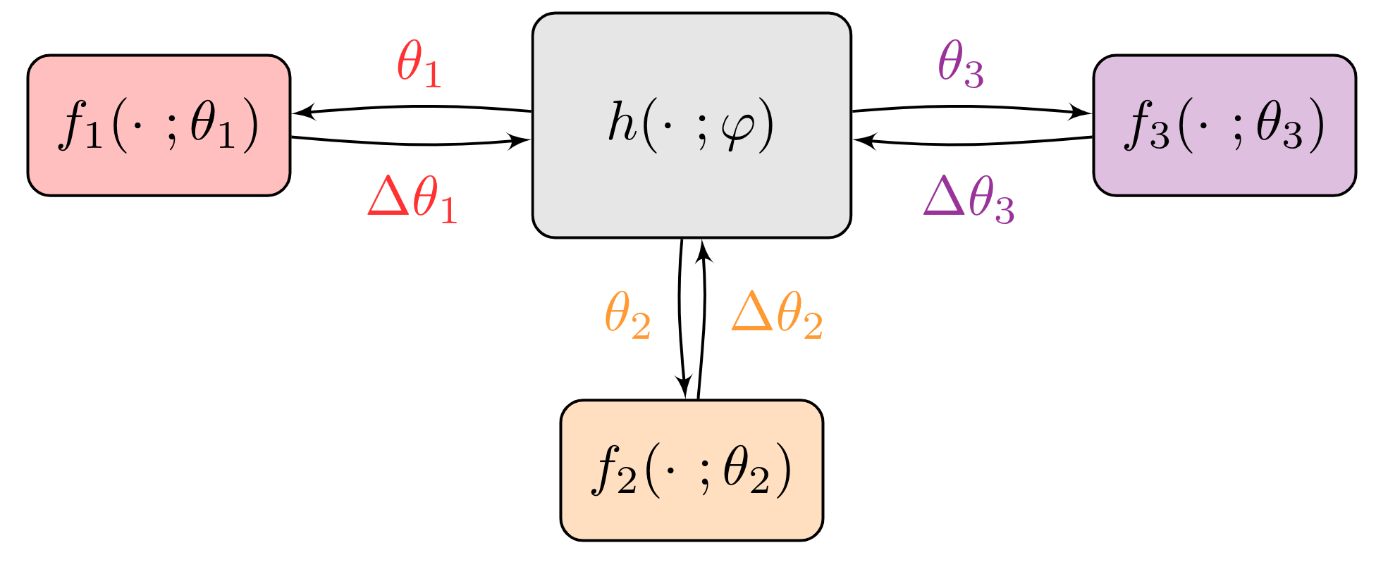
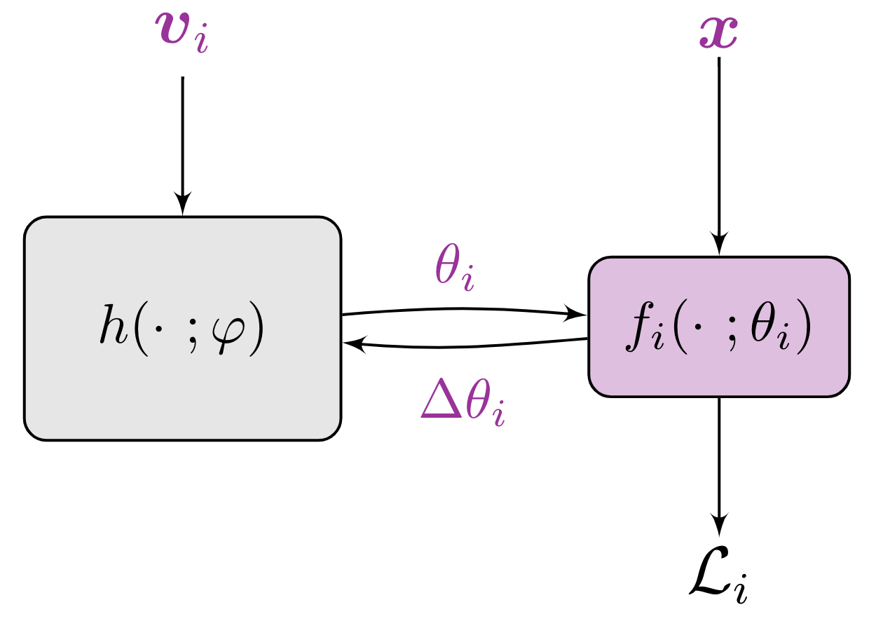
Figure 1: The Federated hypernetwork framework. (a) An HN is located on the server and communicate personal model for each clients. In turn, the clients send back the update direction $\Delta\theta_{i}$; (b) The HN acts on the client embedding $\bm{v}_{i}$ to produce model weights $\theta_{i}$. The client performs several local optimization steps to obtain $\tilde{\theta}_{i}$, and sends back the update direction $\Delta\theta_{i}=\tilde{\theta}_{i}-\theta_{i}$.

2 Related Work

2.1 Federated Learning

Federated learning (FL) (McMahan et al., 2017a; Kairouz et al., 2019; Mothukuri et al., 2021; Li et al., 2019, 2020a) is a learning setup in machine learning in which multiple clients collaborate to solve a learning task while maintaining privacy and communication efficiency. Recently, numerous methods have been introduced for solving the various FL challenges. Duchi et al. (2014); McMahan et al. (2017b); Agarwal et al. (2018); Zhu et al. (2019) proposed new methods for preserving privacy, and Reisizadeh et al. (2020); Dai et al. (2019); Basu et al. (2020); Li et al. (2020b); Stich (2018) focused on reducing communication cost. While some methods assume a homogeneous setup, in which all clients share a common data distribution (Wang & Joshi, 2018; Lin et al., 2018), others tackle the more challenging heterogeneous setup in which each client is equipped with its own data distribution (Zhou & Cong, 2017; Hanzely & Richtárik, 2020; Zhao et al., 2018; Sahu et al., 2018; Karimireddy et al., 2019; Haddadpour & Mahdavi, 2019; Hsu et al., 2019).

Perhaps the most known and commonly used FL algorithm is FedAvg (McMahan et al., 2017a). It learns a global model by aggregating local models trained on IID data. However, the above methods learn a shared global model for all clients instead of personalized per-client solutions.

2.2 Personalized Federated Learning

The federated learning setup presents numerous challenges including data heterogeneity (differences in data distribution), device heterogeneity (in terms of computation capabilities, network connection, etc.), and communication efficiency (Kairouz et al., 2019). Especially data heterogeneity makes it hard to learn a single shared global model that applies to all clients. To overcome these issues, Personalized Federated Learning (PFL) aims to personalize the global model for each client in the federation (Kulkarni et al., 2020). Many papers proposed a decentralized version of the model agnostic meta-learning (MAML) problem  (Fallah et al., 2020a; Li et al., 2017; Behl et al., 2019; Zhou et al., 2019; Fallah et al., 2020b). Since MAML approach relies on the Hessian matrix, which is computationally costly, several works attempted to approximate the Hessian (Finn et al., 2017; Nichol et al., 2018). Another approach to PFL is model mixing where the clients learn a mixture of the global and local models (Deng et al., 2020; Arivazhagan et al., 2019). Hanzely & Richtárik (2020) introduced a new neural network architecture that is divided into base and personalized layers. The central model trains the base layers by FedAvg and the personalized layers (also called top layers) are trained locally. Liang et al. (2020) presented LG-FedAvg a mixing model where each client obtains local feature extractor and global output layers. This is an opposite approach to the conventional mixing model that enables lower communication costs as the global model requires fewer parameters. Other approaches to train the global and local models under different regularization (Huang et al., 2020). Dinh et al. (2020) introduced pFedMe, a method that uses Moreau envelops as the client regularized loss. This regularization helps to decouple the personalized and global model optimizations. Alternatively, clustering methods for federated learning assume that the local data of each client is partitioned by nature (Mansour et al., 2020). Their goal is to group together similar clients and train a centralized model per group. In case of heterogeneous setup, some clients are ”closer” than others in terms of data distribution. Based on this assumption and inspired by FedAvg, Zhang et al. (2020) proposed pFedFOMO, an aggregation method where each client only federates with a subset of relevant clients.

2.3 Hypernetworks

Hypernetworks (HNs) (Klein et al., 2015; Riegler et al., 2015; Ha et al., 2017) are deep neural networks that output the weights of another target network, that performs the learning task. The idea is that the output weights vary depending on the input to the hypernetwork.

HNs are widely used in various machine learning domains, including language modeling (Suarez, 2017), computer vision (Ha et al., 2017; Klocek et al., 2019), continual learning (von Oswald et al., 2019), hyperparameter optimization (Lorraine & Duvenaud, 2018; MacKay et al., 2019; Bae & Grosse, 2020), multi-objective optimization (Navon et al., 2021), and decoding block codes (Nachmani & Wolf, 2019).

HNs are naturally suitable for learning a diverse set of personalized models, as HNs dynamically generate target networks conditioned on the input.

3 Method

In this section, we first formalize the personalized federated learning (PFL) problem, then we present our personalized Federated HyperNetworks (pFedHN) approach.

3.1 Problem Formulation

Personalized federated learning (PFL) aims to collaboratively train personalized models for a set of $n$ clients, each with its own personal private data. Unlike conventional FL, each client $i$ is equipped with its own data distribution ${\mathcal{P}}_{i}$ on $\mathcal{X}\times\mathcal{Y}$. Assume each client has access to $m_{i}$ IID samples from ${\mathcal{P}}_{i}$, ${\mathcal{S}}_{i}=\{(\bm{x}_{j}^{(i)},y_{j}^{(i)})\}_{i=1}^{m_{i}}$. Let $\ell_{i}:\mathcal{Y}\times\mathcal{Y}\to\mathbb{R}_{+}$ denote the loss function corresponds to client $i$, and ${\mathcal{L}}_{i}$ the average loss over the personal training data ${\mathcal{L}}_{i}(\theta_{i})=\frac{1}{m_{i}}\sum_{j}\ell_{i}(\bm{x}_{j},y_{j};\theta_{i})$. Here $\theta_{i}$ denotes the personal model of client $i$. The PFL goal is to optimize

$$\Theta^{*}=\arg\min_{\Theta}\frac{1}{n}\sum_{i=1}^{n}\mathbb{E}_{\bm{x},y\sim{\mathcal{P}}_{i}}[\ell_{i}(\bm{x}_{j},y_{j};\theta_{i})]$$ (1)

and the training objective is given by

$$\arg\min_{\Theta}\frac{1}{n}\sum_{i=1}^{n}{\mathcal{L}}_{i}(\theta_{i})=\arg\min_{\Theta}\frac{1}{n}\sum_{i=1}^{n}\frac{1}{m_{i}}\sum_{j=1}^{m_{i}}\ell_{i}(\bm{x}_{j},y_{j};\theta_{i})$$ (2)

where $\Theta$ denotes the collection of all personal model parameters $\{\theta_{i}\}_{i=1}^{n}$.

3.2 Federated Hypernetworks

In this section, we describe our proposed personalized Federated Hypernetworks (pFedHN), a novel method for solving the PFL problem (eq. 2) using hypernetworks. Hypernetworks are deep neural networks that output the weights of another network, conditioning on its input. Intuitively, HNs simultaneously learn a family of target networks. Let $h(\cdot;\varphi)$ denote the hypernetwork parametrized by $\varphi$ and $f(\cdot;\theta)$ the target network parametrized by $\theta$. The hypernetwork is located at the server and acts on a client descriptor $\bm{v}_{i}$ (see Figure 1). The descriptor can be a trainable embedding vector for the client or fixed, provided that a good client representation is known a-priori. Given $\bm{v}_{i}$ the HN outputs the weights for the $i^{th}$ client $\theta_{i}=\theta_{i}(\varphi):=h(\bm{v}_{i};\varphi)$. Hence, the HN $h$ learns a family of personalized models $\{h(\bm{v}_{i};\varphi)\mid i\in[n]\}$. pFedHN provides a natural way for sharing information across clients while maintaining the flexibility of personalized models, by sharing the parameters $\varphi$.

We adjust the PFL objective (eq. 2) according to the above setup to obtain

$$\arg\min_{\varphi,\bm{v}_{1},...,\bm{v}_{n}}\frac{1}{n}\sum_{i=1}^{n}{\mathcal{L}}_{i}(h(\bm{v}_{i};\varphi)).$$ (3)

One crucial and attractive property of pFedHN is that it decouples the size of $h$ and the communication cost. The amount of data transferred is determined by the size of the target network during the forward and backward communications, and does not depend on the size of $h$. Consequently, the hypernetwork can be arbitrarily large without impairing communication efficiency. Indeed, using the chain rule we have $\nabla_{\varphi}{\mathcal{L}}_{i}=(\nabla_{\varphi}\theta_{i})^{T}\nabla_{\theta_{i}}{\mathcal{L}}_{i}$ so the client only needs to communicate $\nabla_{\theta_{i}}{\mathcal{L}}_{i}$ back to the hypernetwork, which has the same size as the personal network parameters $\theta_{i}$.

In our work, we used a more general update rule $\Delta\varphi=(\nabla_{\varphi}\theta_{i})^{T}\Delta\theta_{i}$ where $\Delta\theta_{i}$ is the change in the local model parameters after several local update steps. As the main limitation is the communication cost, we found it beneficial to perform several local update steps, on the client side per communication round. This aligns with prior work that highlighted the benefits of local optimization steps in terms of both convergence speed (hence communication cost) and final accuracy (McMahan et al., 2017a; Huo et al., 2020). Given the current personalized parameters $\theta_{i}$, we perform several local optimization steps on the personal data to obtain $\tilde{\theta}_{i}$. We then return the personal model update direction $\Delta\theta_{i}:=\tilde{\theta}_{i}-\theta_{i}$ therefore, the update for $\varphi$ is given by $(\nabla_{\varphi}\theta_{i})^{T}(\tilde{\theta}_{i}-\theta_{i})$. This update rule is inspired by Zhang et al. (2019). Intuitively, suppose we have access to the optimal solution of the personal problem $\theta_{i}^{*}=\arg\min_{\theta_{i}}{\mathcal{L}}_{i}$, then our update rule becomes the gradient of an approximation to the surrogate loss $\tilde{{\mathcal{L}}}_{i}(\bm{v}_{i},\varphi)=\frac{1}{2}||\theta_{i}^{*}-h(\bm{v}_{i};\varphi)||^{2}_{2}$ by replacing $\theta_{i}^{*}$ with $\tilde{\theta}_{i}$. In Appendix B (Figure 5), we compare the results for a different number of local update steps and show considerable improvement over using the gradient, i.e., using a single step.

Algorithm 1 Personalized Federated Hypernetwork

input: $R$ — number of rounds, $K$ — number of local rounds, $\alpha$ — learning rate, $\eta$ — client learning rate

for $r=1,...,R$ do

    sample client $i\in[n]$

    set $\theta_{i}=h(\bm{v}_{i};\varphi)$ and $\tilde{\theta}_{i}=\theta_{i}$

    for $k=1,...,K$ do

         sample mini-batch $B\subset{\mathcal{S}}_{i}$

         $\tilde{\theta}_{i}=\tilde{\theta}_{i}-\eta\nabla_{\tilde{\theta}_{i}}{\mathcal{L}}_{i}(B)$     

    $\Delta\theta_{i}=\tilde{\theta}_{i}-\theta_{i}$

    $\varphi=\varphi-\alpha\nabla_{\varphi}\theta_{i}^{T}\Delta\theta_{i}$

    $\bm{v}_{i}=\bm{v}_{i}-\alpha\nabla_{\bm{v}_{i}}\varphi^{T}\nabla_{\varphi}\theta_{i}^{T}\Delta\theta_{i}$

return: $\varphi$

3.3 Personal Classifier

In some cases, it is undesirable to learn the entire network end-to-end with a single hypernetwork. As an illustrative example, consider a case where clients differ only by the label ordering in their output vectors. In this case, having to learn the right label ordering per client adds another unnecessary difficulty if they were to learn the classification layer as well using the hypernetwork.

As another example, consider the case where each client solves an entirely separate task, similar to multitask learning, where the number of classes may differ between clients. It makes little sense to have the hypernetwork produce each unique task classification layer.

In these cases, it would be preferable for the hypernetwork to produce the feature extraction part of the target network, which contains most of the trainable parameters, while learning a local output layer for each client. Formally, let $\omega_{i}$ denote the personal classifier parameters of client $i$. We modify the optimization problem (eq.  3) to obtain,

$$\arg\min_{\varphi,\bm{v}_{1},...,\bm{v}_{n},\omega_{1},...,\omega_{n}}\frac{1}{n}\sum_{i=1}^{n}{\mathcal{L}}_{i}(\theta_{i},\omega_{i}),$$ (4)

where we define the feature extractor $\theta_{i}=h(\bm{v}_{i};\varphi)$, as before. The parameters $\varphi,\bm{v}_{1},...,\bm{v}_{n}$ are updated according to Alg. 1, while the personal parameters $\omega_{i}$ are updated locally using

$$\omega_{i}=\omega_{i}-\alpha\nabla_{\omega_{i}}{\mathcal{L}}_{i}.$$

4 Analysis

In this section, we theoretically analyze pFedHN. First, we provide an insight regarding the solution for the pFedHN (Eq. 3), using a simple linear version of our hypernetwork. Next, we describe the generalization bounds of our framework.

4.1 A Linear Model

Consider a linear version of the hypernetwork, where both the target model and the hypernetwork are linear models, $\theta_{i}=W\bm{v}_{i}$ with $\varphi:=W\in{\mathbb{R}}^{d\times k}$ and $\bm{v}_{i}\in{\mathbb{R}}^{k}$ is the $i^{th}$ clients embedding. Let $V$ denote the $k\times n$ matrix whose columns are the clients embedding vectors $\bm{v}_{i}$. We note that even for convex loss functions ${\mathcal{L}}_{i}(\theta_{i})$ the objective ${\mathcal{L}}(W,V)=\sum_{i}{\mathcal{L}}_{i}(W\bm{v}_{i})$ might not be convex in $(W,V)$ but block multi-convex. In one setting, however, we get a nice analytical solution.

Proposition 1.

Let $\{X_{i},\bm{y}_{i}\}$ be the data for client $i$ and let the loss for linear regressor $\theta_{i}$ be ${\mathcal{L}}_{i}(\theta_{i})=\|X_{i}\theta_{i}-\bm{y}_{i}\|^{2}$. Furthermore assume for all $i$, $X_{i}^{T}X_{i}=I_{d}$. Define the empirical risk minimization (ERM) solution for client $i$ as $\bar{\theta}_{i}=\arg\min_{\theta\in{\mathbb{R}}^{d}}\|X_{i}\theta-\bm{y}_{i}\|^{2}$. The optimal $W,V$ minimizing $\sum_{i}\|X_{i}W\bm{v}_{i}-\bm{y}_{i}\|^{2}$ are given by PCA on $\{\bar{\theta}_{1},...,\bar{\theta}_{n}\}$, where $W$ is the top $k$ principle components and $\bm{v}_{i}$ is the coefficients for $\bar{\theta}_{i}$ in these components.

We provide the proof in Section A of the Appendix. The linear version of our pFedHN performs dimensionality reduction by PCA, but unlike classical dimensionality reduction which is unaware of the learning task, pFedHN uses multiple clients for reducing the dimensionality while preserving the optimal model as best as possible. This allows us to get solutions between the two extremes: A single shared model up to scaling ($k=1$) and each client training locally ($k\geq n$). We note that optimal reconstruction of the local models ($k\geq n$) is generally suboptimal in terms of generalization performance, as no information is shared across clients.

This dimensionality reduction can also be viewed as a denoising process. Assume a linear regression with Gaussian noise model, i.e., for all clients $p(y|x)=\mathcal{N}(x^{T}\theta_{i}^{*},\sigma^{2})$ and that each client solves a maximum likelihood objective. From the central limit theorem for maximum likelihood estimators (White, 1982) we get that $\sqrt{n_{i}}(\bar{\theta}_{i}-\theta^{*}_{i})\overset{d}{\longrightarrow}\mathcal{N}(0,I_{d})$ where $\bar{\theta}_{i}$ is the maximum likelihood solution. This means that approximately $\bar{\theta}_{i}=\theta^{*}_{i}+\epsilon$ with $\epsilon\sim\mathcal{N}(0,\sigma_{i}I)$, i.e., our local solutions $\bar{\theta}_{i}$ are a noisy version of the optimal model $\theta^{*}_{i}$ with isotropic Gaussian noise.

We can now view the linear hypernetworks as performing denoising on $\bar{\theta}_{i}$, by PCA. PCA is a classic approach to denoising (Muresan & Parks, 2003) and is well suited for reducing isotropic noise when the energy of the original points is concentrated on a small dimensional subspace. Intuitively we think of our standard hypernetwork as a nonlinear extension of this approach, which has a similar effect by forcing the models to lay on a low-dimensional manifold.

Table 1: Heterogeneous data. Test accuracy over $10,50,100$ clients on the CIFAR10, CIFAR100, and Omniglot datasets.

	CIFAR10				CIFAR100				Omniglot
# clients	10	50	100		10	50	100		50
Local	$86.46\pm 4.02$	$68.11\pm 7.39$	$59.32\pm 5.59$		$58.98\pm 1.38$	$19.98\pm 1.41$	$15.12\pm 0.58$		$65.97\pm 0.86$
FedAvg	$51.42\pm 2.41$	$47.79\pm 4.48$	$44.12\pm 3.10$		$15.96\pm 0.55$	$15.71\pm 0.35$	$14.59\pm 0.40$		$41.61\pm 3.59$
Per-FedAvg	$76.65\pm 4.84$	$83.03\pm 0.25$	$80.19\pm 1.99$		$50.14\pm 1.06$	$45.89\pm 0.76$	$48.28\pm 0.70$		$76.46\pm 0.17$
FedPer	$87.27\pm 1.39$	$83.39\pm 0.47$	$80.99\pm 0.71$		$55.76\pm 0.34$	$48.32\pm 1.46$	$42.08\pm 0.18$		$69.92\pm 3.12$
pFedMe	$87.69\pm 1.93$	$86.09\pm 0.32$	$85.23\pm 0.58$		$51.97\pm 1.29$	$49.09\pm 1.10$	$45.57\pm 1.02$		$69.98\pm 0.28$
LG-FedAvg	$89.11\pm 2.66$	$85.19\pm 0.58$	$81.49\pm 1.56$		$53.69\pm 1.42$	$53.16\pm 2.18$	$49.99\pm 3.13$		$72.99\pm 5.00$
pFedHN (ours)	$90.83\pm 1.56$	$88.38\pm 0.29$	$87.97\pm 0.70$		$65.74\pm 1.80$	$59.48\pm 0.67$	$\mathbf{53.24\pm 0.31}$		$72.03\pm 1.08$
pFedHN-PC (ours)	$\mathbf{92.47\pm 1.63}$	$\mathbf{90.08\pm 0.63}$	$\mathbf{88.09\pm 0.86}$		$\mathbf{68.15\pm 1.49}$	$\mathbf{60.17\pm 1.63}$	$52.4\pm 0.74$		$\mathbf{81.89\pm 0.15}$

4.2 Generalization

We now investigate how pFedHN generalizes using the approach of Baxter (2000). The common approach for multi-task learning with neural networks is to have a common feature extractor shared by all tasks and a per-task head operating on these features. This case was analyzed by Baxter (2000). Conversely, here the per-task parameters are the inputs to the hypernetwork. Next, we provide the generalization guarantee under this setting and discuss its implications.

Let $D_{i}=\left\{(\bm{x}^{(i)}_{j},y^{(i)}_{j})\right\}_{j=1}^{m}$ be the training set for the $i^{th}$ client, generated by a distribution $P_{i}$. We denote by $\hat{\mathcal{L}}_{D}(\varphi,V)$ the empirical loss of the hypernetwork $\hat{\mathcal{L}}_{D}(\varphi,V)=\frac{1}{n}\sum_{i=1}^{n}\frac{1}{m}\sum_{j=1}^{m}\ell_{i}\left(\bm{x}^{(i)}_{j},y^{(i)}_{j};h(\varphi,\bm{v}_{i})\right)$ and by ${\mathcal{L}}(\varphi,V)$ the expected loss ${\mathcal{L}}(\varphi,V)=\frac{1}{n}\sum_{i=1}^{n}\mathbb{E}_{P_{i}}\left[\ell_{i}(\bm{x},y;h(\varphi,\bm{v}_{i}))\right]$.

We assume weights of the hypernetwork and the embeddings are bounded in a ball of radius $R$, in which the following three Lipschitz conditions hold:

1. $|\ell_{i}(\bm{x},y,\theta_{1})-\ell_{i}(\bm{x},y,\theta_{2})|\leq L\|\theta_{1}-\theta_{2}\|$

2. $\|h(\varphi,\bm{v})-h(\varphi^{\prime},\bm{v})\|\leq L_{h}\|\varphi-\varphi^{\prime}\|$

3. $\|h(\varphi,\bm{v})-h(\varphi,\bm{v}^{\prime})\|\leq L_{V}\|\bm{v}-\bm{v}^{\prime}\|$.

Theorem 1.

Let the hypernetwork parameter space be of dimension $N$ and the embedding space be of dimension $k$. Under previously stated assumptions, there exists $M=\mathcal{O}\left(\frac{k}{\epsilon^{2}}\log\left(\frac{RL(L_{h}+L_{V})}{\delta}\right)+\frac{N}{n\epsilon^{2}}\log\left(\frac{RL(L_{h}+L_{V})}{\delta}\right)\right)$ such that if the number of samples per client $m$ is greater than $M$, we have with probability at least $1-\delta$ for all $\varphi,V$ that $|\mathcal{L}(\varphi,V)-\hat{\mathcal{L}}_{D}(\varphi,V)|\leq\epsilon.$

Theorem 1 provides insights on the parameter-sharing effect of pFedHN. The first term for the number of required samples $M$ depends on the dimension of the embedding vectors; as each client corresponds to its unique embedding vector (i.e. not being shared between clients), this part is independent of the number of clients $n$. However, the second term depends on the size of the hypernetwork $N$, is reduced by a factor $n$, as the hypernetwork’s weights are shared.

Additionally, the generalization is affected by the Lipschitz constant of the hypernetwork, $L_{h}$ (along with other Lipschitz constants), as it can affect the effective space we can reach with our embedding. In essence, this characterizes the price that we pay, in terms of generalization, for the hypernetworks flexibility. It might also open new directions to improve performance. However, our initial investigation into bounding the Lipschitz constant by adding spectral normalization (Miyato et al., 2018) did not show any significant improvement, see Appendix C.

5 Experiments

We evaluate pFedHN in several learning setups using three common image classification datasets: CIFAR10, CIFAR100, and Omniglot (Krizhevsky & Hinton, 2009; Lake et al., 2015) Unless stated otherwise, we report the Federated Accuracy, defined as $\frac{1}{n}\sum_{i}\frac{1}{m_{i}}\sum_{j}\text{Acc}\left(f_{i}\left(\bm{x}^{(i)}_{j}\right),y^{(i)}_{j}\right)$, averaged over three seeds. The experiments show that pFedHN outperforms classical FL approaches and leading PFL models.

Compared Methods:

We evaluate and compare the following approaches: (1) pFedHN, Our proposed Federated HyperNetworks (2) pFedHN-PC, pFedHN with a personalized classifier per client ; (3) Local, Local training on each client, with no collaboration between clients; (4) FedAvg (McMahan et al., 2017a), one of the first and perhaps the most widely used FL algorithm; (5) Per-FedAvg (Fallah et al., 2020a) a meta-learning based PFL algorithm. (6) pFedMe (Dinh et al., 2020), a PFL approach which adds a Moreau-envelopes loss term; (7) LG-FedAvg (Liang et al., 2020) PFL method with local feature extractor and global output layers; (8) FedPer (Arivazhagan et al., 2019) a PFL approach that learns per-client personal classifier on top of a shared feature extractor.

Training Strategies:

In all experiments, our target network shares the same architecture as the baseline models. Our hypernetwork is a simple fully-connected neural network, with three hidden layers and multiple linear heads per target weight tensor. We limit the training process to at-most $5000$ server-client communication steps for most methods. One exception is LG-FedAvg which utilizes a pretrained FedAvg model, hence it is trained with additional $1000$ communication steps. The Local baseline is trained for $2000$ optimization steps on each client. For pFedHN, we set the number of local steps to $K=50$, and the embedding dimension to $\lfloor 1+n/4\rfloor$, where $n$ is the number of clients. We provide an extensive ablation study on design choices in Appendix C. We tune the hyperparameters of all methods using a pre-allocated held-out validation set. Full experimental details are provided in Appendix B.

5.1 Heterogeneous Data

We evaluate the different approaches on a challenging heterogeneous setup. We adopt the learning setup and the evaluation protocol described in Dinh et al. (2020) for generating heterogeneous clients in terms of classes and size of local training data. First, we sample two/ten classes for each client for CIFAR10/CIFAR100; Next, for each client $i$ and selected class $c$, we sample $\alpha_{i,c}\sim U(.4,.6)$, and assign it with $\frac{\alpha_{i,c}}{\sum_{j}\alpha_{j,c}}$ of the samples for this class. We repeat the above using $10,50$ and $100$ clients. This procedure produces clients with different number of samples and classes. For the target network, we use a LeNet-based (LeCun et al., 1998) network with two convolution and two fully connected layers.

We also evaluate all methods using the Omniglot dataset (Lake et al., 2015). Omniglot contains 1623 different grayscale handwritten characters (with 20 samples each), from 50 different alphabets. Each alphabet obtains a varying number of characters. In this setup, we use 50 clients and assign an alphabet to each client. Therefore, clients receives different numbers of samples and the distribution of labels is disjoint across clients. We use a LeNet-based model with four convolution and two fully connected layers.

The results are presented in Table 1. The two simple baselines, local and FedAvg, that do not use personalized federated learning perform quite poorly on most tasks, showing the importance of personalized federated learning. pFedHN achieves large improvements of 2%-10% over all competing approaches. Furthermore, on the Omniglot dataset, where each client is allocated with a completely different learning task (different alphabet), we show significant improvement using pFedHN-PC. We present additional results on the MNIST dataset in Appendix C.

5.2 Computational Budget

Table 2: Computational budget. Test accuracy for CIFAR10/100 with 75 clients and varying computational capacities.

	CIFAR10				CIFAR100
Local model size	S	M	L		S	M	L
FedAvg	$36.91\pm 2.26$	$42.09\pm 2.37$	$47.51\pm 1.97$		$9.79\pm 0.19$	$11.76\pm 1.14$	$17.86\pm 2.42$
Per-FedAvg	$70.72\pm 2.57$	$72.33\pm 2.57$	$75.13\pm 0.61$		$41.49\pm 0.91$	$43.22\pm 0.16$	$44.03\pm 1.77$
pFedMe	$81.21\pm 1.23$	$84.08\pm 1.63$	$83.15\pm 2.45$		$39.91\pm 0.81$	$41.99\pm 0.55$	$44.93\pm 1.63$
LG-FedAvg	$73.93\pm 3.65$	$53.13\pm 3.49$	$54.72\pm 2.50$		$33.48\pm 4.83$	$29.15\pm 1.51$	$23.01\pm 1.41$
pFedHN (ours)	$\mathbf{85.38\pm 1.21}$	$\mathbf{86.92\pm 1.35}$	$\mathbf{87.20\pm 0.76}$		$\mathbf{48.04\pm 0.89}$	$\mathbf{48.66\pm 1.21}$	$\mathbf{50.66\pm 2.70}$

We discussed above how the challenges of heterogeneous data can be handled using pFedHN. Another major challenge presented by personalized FL is that the communication, storage, and computational resources of clients may differ significantly. These capacities may even change in time due to varying network and power conditions. In such a setup, the server should adjust to the communication and computational policies of each client. Unfortunately, previous works do not address this resource heterogeneity. pFedHN can naturally adapt to this challenging learning setup by producing target networks of different sizes.

In this section, we evaluate the capacity of pFedHN to handle clients that differ in their computational and communication resource budget. We use the same split described in Section 5.1 with a total of $75$ clients divided into the three equal-sized groups named S (small), M (medium), and L (large). The Models of clients within each group share the same architecture. The three architectures (of the three groups) have a different number of parameters.

We train a single pFedHN to output target client models of different sizes. Importantly, this allows pFedHN to share parameters between all clients even if those have different local model sizes.

Baselines: For quantitative comparisons, and since the existing baseline methods cannot easily extend to this setup, we train three independent per-group models. Each group is trained for $5000$ server-client communication steps. See details in Appendix C for further details.

The results are presented in Table 2, showing that pFedHN achieves $4\%-8\%$ improvement over all competing methods. The results demonstrate the flexibility of our approach, which is capable of adjusting to different client settings while maintaining high accuracy.

5.3 Generalization to Novel Clients

Next, we study an important learning setup where new clients join, and a new model has to be trained for their data. In the general case of sharing models across clients, this would require retraining (or finetuning) the shared model. While PFL methods like pFedME (Dinh et al., 2020) and Per-FedAvg (Fallah et al., 2020a) can adapt to this setting by finetuning the global model locally, pFedHN architecture offers a significant benefit. Since the shared model learns a meta-model over the distribution of clients, it can in principle generalize to new clients without retraining. With pFedHN, once the shared model $\varphi$ has been trained on a set of clients, extending to a new set of novel clients requires little effort. We freeze the hypernetwork weights $\varphi$ and optimize an embedding vector $\bm{v}_{new}$. Since only a small number of parameters are being optimized, training is less prone to overfitting compared to other approaches. The success of this process depends on the capacity of the hypernetwork to learn the distribution over clients and generalize to clients that have different data distributions.

To evaluate pFedHN in this setting, we use the CIFAR10 dataset, with a total of 100 clients, of which 90 are used for training and 10 are held out novel clients. To allocate data samples, for each client $i$ we first draw a sample from a Dirichlet distribution with parameter $\bm{\alpha}=(\alpha,...,\alpha)\in\mathbb{R}^{10}$, $p_{i}\sim Dir(\bm{\alpha})$. Next we normalize the $p_{i}$’s so that $\sum_{i}p_{i,j}=1$ for all $j$, to obtain the vector $\hat{p}_{i}$. We now allocate samples according to the $\hat{p}_{i}$’s. For the training clients, we choose $\alpha=.1$, whereas for the novel clients we vary $\alpha\in\{.1,.25,.5,1\}$. To estimate the “distance” between a novel client and the training clients, we use the total variation (TV) distance between the novel client and its nearest neighbor in the training set. The TV is computed over the empirical distributions $\hat{p}$. Figure 2 presents the accuracy generalization gap as a function of the total variation distance. pFedHN achieves the best generalization performance for all levels of TV (corresponds to the different values for $\mathbb{\alpha}$).

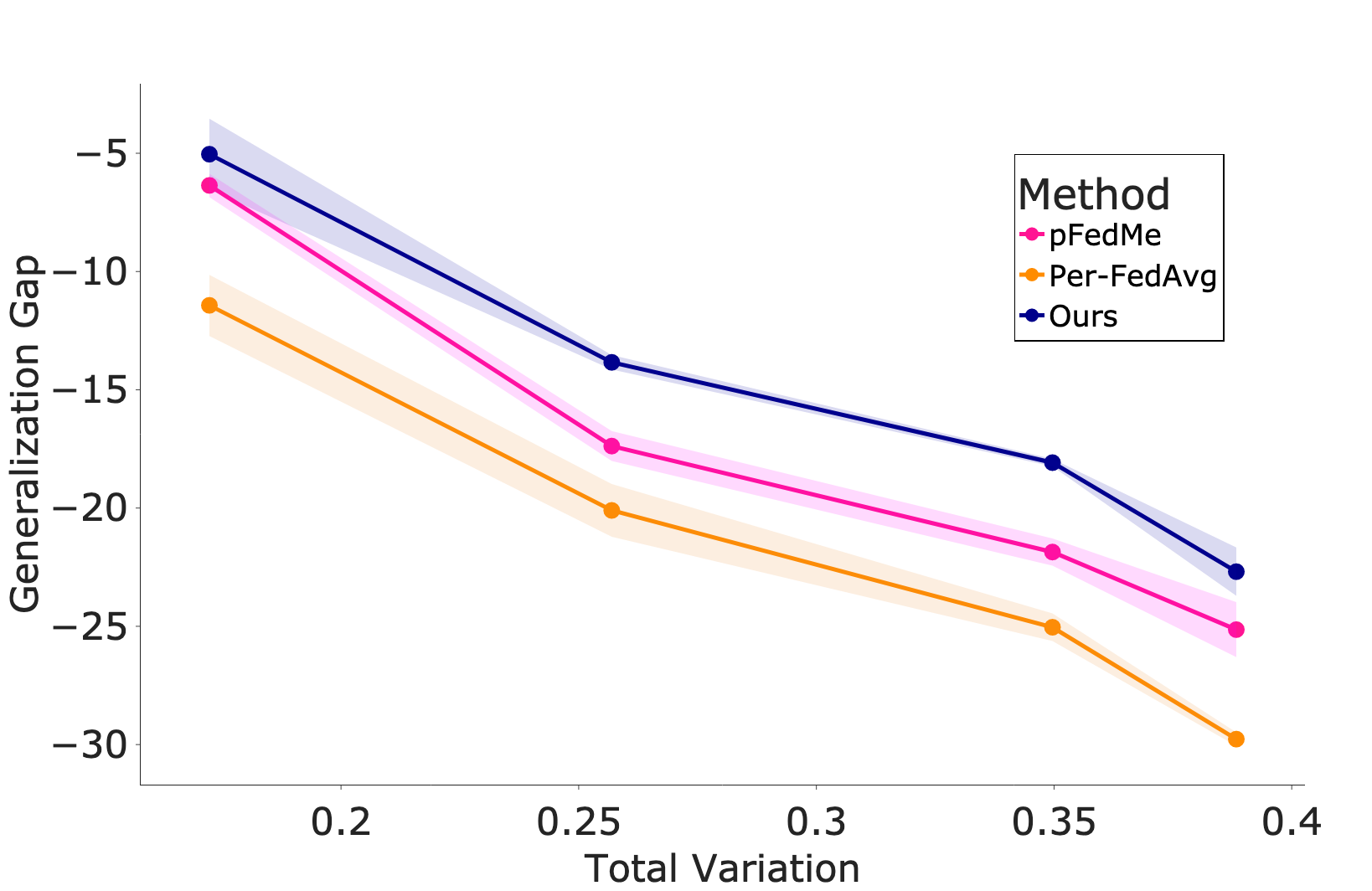
Figure 2: Generalization to novel clients. The accuracy generalization gap between training and novel clients, defined as $\text{acc}_{novel}-\text{acc}_{train}$, where acc denotes the average accuracy.

5.4 Heterogeneity of personalized classifiers

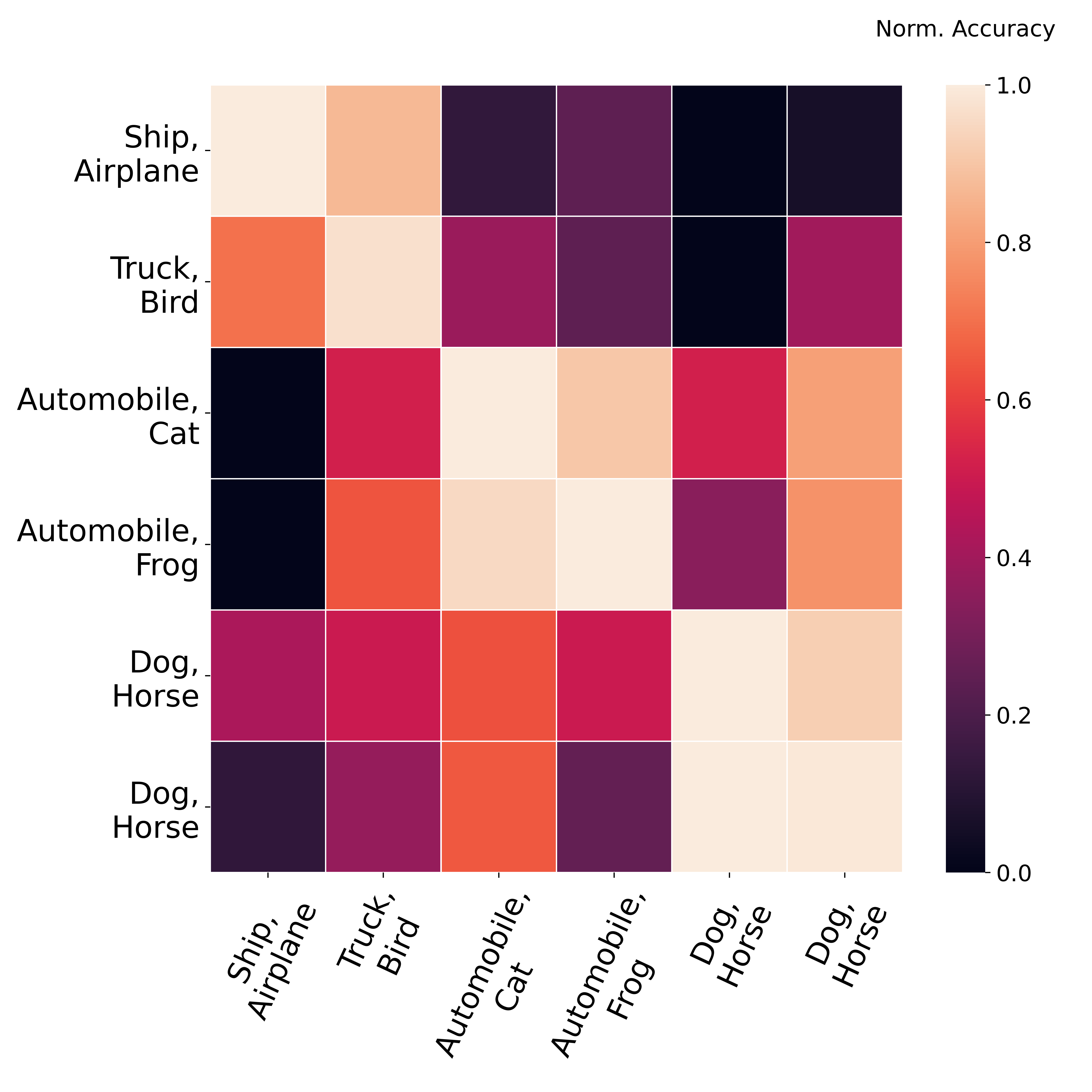
Figure 3: Model personalization. Rows correspond to clients, each with their trained in a binary classification task and keeping their personalized classifier $\omega_{i}$. Columns correspond to the feature extractor $\theta_{j}$ of another client. The diagonal corresponds to the stanard training with $\theta_{i}$ and $\omega_{i}$. For better visualization, values denote accuracy normalized per row: $\text{norm-acc}_{i,j}=(\text{acc}_{i,j}-\min_{\ell}{\text{acc}_{i,\ell}})/(\max_{\ell}{\text{acc}_{i,\ell}}-\min_{\ell}{\text{acc}_{i,\ell}})$.

We further investigate the flexibility of pFedHN-PC in terms of personalizing different networks for different clients. Potentially, since clients have their own personalized classifier $\omega_{i}$, the feature extractor component $\theta_{i}$ generated by the HN may in principle become strongly similar across clients, making the HN redundant. The empirical results show that this is not the case because pFedHN-PC out-performs FedPer (Arivazhagan et al., 2019). However this raises a fundamental question about the interplay between local and shared personalized components. We provide additional insight to this topic by answering the question: do the feature extraction layers generated by the pFedHN-PC’s hypernetwork significantly differ from each other?

To investigate the level of personalization in $\theta_{i}$ achieved by pFedHN-PC, we first train it on CIFAR10 dataset split among ten clients, with two classes assigned to each client. Next, for each client, we replace its feature extractor $\theta_{i}$ with that of another client $\theta_{j}$ while keeping its personal classifier $\omega_{i}$ unaltered. Figure 3 depicts the normalized accuracy in this mix-and-match experiment. Rows correspond to a client, and columns correspond to the feature extractor of another client.

Several effects in Figure 3 are of interest. First, pFedHN-PC produces personalized feature extractors for each client since the accuracy achieved when crossing classifiers and feature extractors varies significantly. Second, some pairs of clients can be crossed without hurting the accuracy. Specifically, we had two clients learning to discriminate horse vs. dog. Interestingly, the client with ship and airplane classes performs quite well when presented with truck and bird, presumably because both of their feature extractors learned to detect sky.

5.5 Learned Client Representation

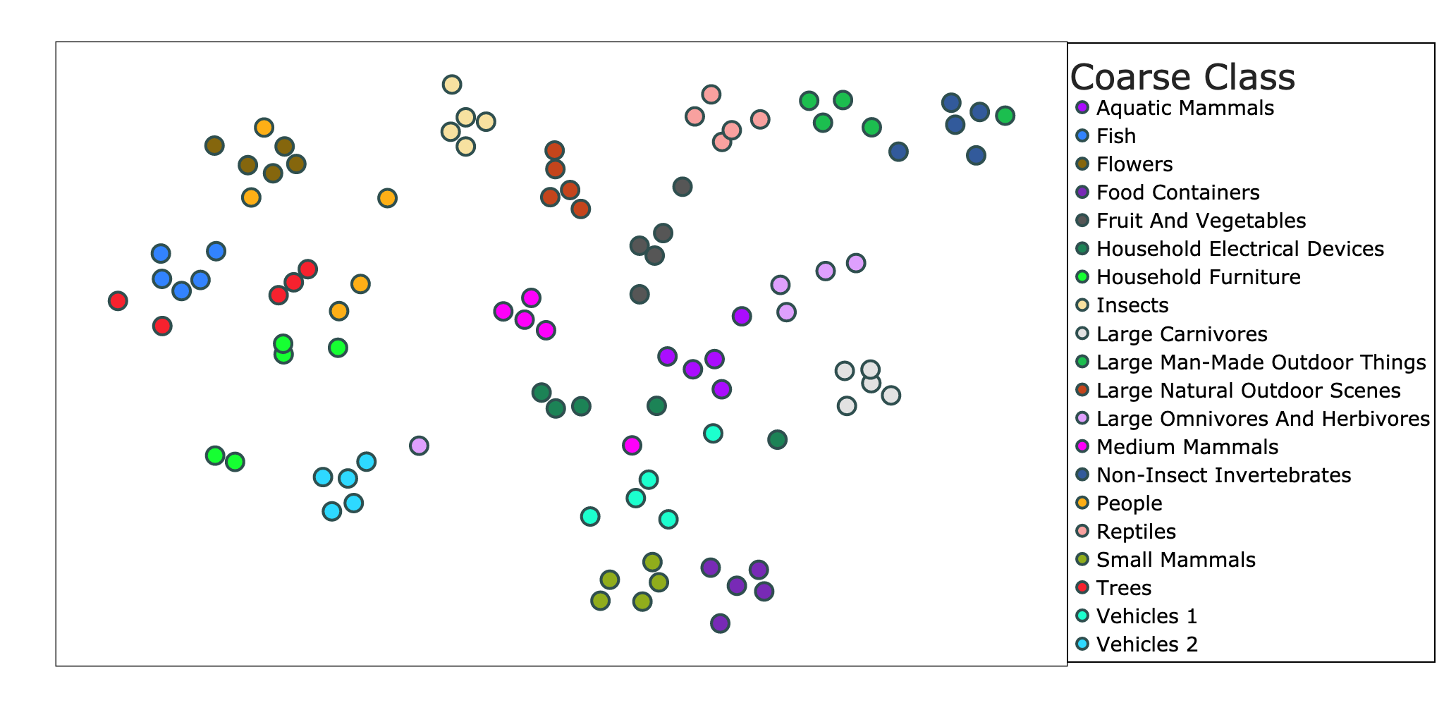
Figure 4: t-SNE visualization of the learned client representation $\bm{v}$ for the CIFAR100 dataset. Clients are tasked with classifying classes that belong to the same coarse class. Clients marked with the same color correspond to the same coarse-class, see text for details. pFedHN clustered together clients from the same group.

In our experiments, we learn to represent each client using a trainable embedding vector $v_{i}$. These embedding vectors therefore learn a continuous semantic representation over the set of clients. The smooth nature of this representation gives the HN the power to share information across clients. We now wish to study the structure of that embedding space.

To examine how the learned embedding vectors reflect a meaningful representation over the client space, we utilize the hierarchy in CIFAR100 for generating clients with similar data distribution of semantically similar labels. Concretely, we split the CIFAR100 into 100 clients, where each client is assigned with data from one out of the twenty coarse classes uniformly (i.e., each coarse class is assigned to five clients).

In Figure 4 we project the learned embedding vectors into $\mathbb{R}^{2}$ using the t-SNE algorithm (Maaten & Hinton, 2008). A clear structure is presented, in which clients from the same group (in terms of coarse labels) are clustered together.

6 Conclusion

In this work, we present a novel approach for personalized federated learning. Our method trains a central hypernetwork to output a unique personal model for each client. We show through extensive experiments significant improvement in accuracy on all datasets and learning setups.

Sharing across clients through a central hypernetwork has several benefits compared to previous architectures. First, since it learns a unified model over the distribution of clients, the model generalizes better to novel clients, without the need to retrain the central model. Second, it naturally extends to handle clients with different compute power, by generating client models of different sizes. Finally, this architecture decouples the problem of training complexity from communication complexity, since local models that are transmitted to clients can be significantly more compact than the central model.

We expect that the current framework can be further extended in several important ways. First, the architecture opens questions about the best way of allocating learning capacity to a central model vs distributed components that are trained locally. Second, the question of generalization to clients with new distribution awaits further analysis.

Appendix A Proof of Results

Proof for Proposition 1.

Let $\bar{\theta}_{i}$ denote the optimal solution at client $i$, then $\bar{\theta}_{i}=(X_{i}^{T}X_{i})^{-1}X_{i}^{T}\bm{y}_{i}=X_{i}^{T}\bm{y}_{i}$. Denote $\theta_{i}=W\bm{v}_{i}$, we have

$$\arg\min_{\theta_{i}}\|X_{i}\theta_{i}-\bm{y}_{i}\|_{2}^{2}=\arg\min_{\theta_{i}}(X_{i}\theta_{i}-\bm{y}_{i})^{T}(X_{i}\theta_{i}-\bm{y}_{i})$$

$$=\arg\min_{\theta_{i}}\theta_{i}^{T}X_{i}^{T}X_{i}\theta_{i}-2\theta_{i}^{T}X_{i}^{T}\bm{y}+\bm{y}_{i}^{T}\bm{y}_{i}$$

$$=\arg\min_{\theta_{i}}\theta_{i}^{T}\theta_{i}-2\langle\theta_{i},\bar{\theta}_{i}\rangle+\bm{y}_{i}^{T}\bm{y}_{i}$$

$$=\arg\min_{\theta_{i}}\theta_{i}^{T}\theta_{i}-2\langle\theta_{i},\bar{\theta}_{i}\rangle+\|\bar{\theta}_{i}\|_{2}^{2}$$

$$=\arg\min_{\theta_{i}}\|\theta_{i}-\bar{\theta}_{i}\|_{2}^{2}$$

Thus, our optimization problem becomes $\arg\min_{W,V}\sum_{i}\|W\bm{v}_{i}-\bar{\theta}_{i}\|_{2}^{2}$.

WLOG, we can optimize $W$ over the set of all matrices with orthonormal columns, i.e. $W^{T}W=I$. Since for each solution $(W,V)$ we can obtain the same loss for $(WR,R^{-1}V)$, and select a $R$ that performs Gram-Schmidt on the columns of $W$. In case of fixed $W$ the optimal solution for $\bm{v}_{i}$ is given by $\bm{v}_{i}^{*}=(W^{T}W)^{-1}W^{T}\bar{\theta}_{i}=W^{T}\bar{\theta}_{i}$. Hence, our optimization problem becomes,

$$\arg\min_{W;W^{T}W=I}\sum_{i}\|WW^{T}\bar{\theta}_{i}-\bar{\theta}_{i}\|_{2}^{2},$$

which is equivalent to PCA on $\{\bar{\theta}_{i}\}_{i}$. ∎

Proof for Theorem 1.

We note a $\log(1/\epsilon)$ factor missing in the statement of Theorem 1 in the paper, the correct statement should use $M=\mathcal{O}\left(\frac{k}{\epsilon^{2}}\log\left(\frac{RL(L_{h}+L_{V})}{\epsilon\delta}\right)+\frac{N}{n\epsilon^{2}}\log\left(\frac{RL(L_{h}+L_{V})}{\epsilon\delta}\right)\right)$.

Using Theorem 4 from (Baxter, 2000) and the notation used in that paper, we get that $M=\mathcal{O}\left(\frac{1}{n\epsilon^{2}}\log\left(\frac{\mathcal{C}(\epsilon,\mathds{H}^{n}_{l})}{\delta}\right)\right)$ where $\mathcal{C}(\epsilon,\mathds{H}^{n}_{l})$ is the covering number for $\mathds{H}^{n}_{l}$. In our case each element of $\mathds{H}^{n}_{l}$ is parametrized by $\varphi,\bm{v}_{1},...,\bm{v}_{n}$ and the distance is given by

$$d((\varphi,\bm{v}_{1},...,\bm{v}_{n}),(\varphi^{\prime},\bm{v}^{\prime}_{1},...,\bm{v}^{\prime}_{n}))=$$ (5)

$$\underset{x_{i},y_{i}\sim P_{i}}{\mathds{E}}\left[\frac{1}{n}\left|\sum\ell(h(\varphi,\bm{v}_{i})(x_{i}),y_{i})-\sum\ell(h(\varphi^{\prime},\bm{v}^{\prime}_{i})(x_{i}),y_{i})\right|\right]$$

From the triangle inequality and our Lipshitz assumptions we get

$$d((\varphi,\bm{v}_{1},...,\bm{v}_{n}),(\varphi^{\prime},\bm{v}^{\prime}_{1},...,\bm{v}^{\prime}_{n}))\leq$$ (6)

$$\sum\frac{1}{n}\underset{x_{i},y_{i}\sim P_{i}}{\mathds{E}}\left[\left|\ell(h(\varphi,\bm{v}_{i})(x_{i}),y_{i})-\ell(h(\varphi^{\prime},\bm{v}^{\prime}_{i})(x_{i}),y_{i})\right|\right]$$

$$\leq L\|h(\varphi,\bm{v}_{i})-h(\varphi^{\prime},\bm{v}^{\prime}_{i})\|$$

$$\leq L\|h(\varphi,\bm{v}_{i})-h(\varphi,\bm{v}^{\prime}_{i})\|+L\|h(\varphi,\bm{v}^{\prime}_{i})-h(\varphi^{\prime},\bm{v}^{\prime}_{i})\|$$

$$\leq L\cdot L_{h}\|\varphi-\varphi^{\prime}\|+L\cdot L_{V}\|\bm{v}-\bm{v}^{\prime}\|$$

Now if we select a covering of the parameter space such that each $\varphi$ has a point $\varphi^{\prime}$ that is $\frac{\epsilon}{2L(L_{h}+L_{V})}$ away and each embedding $\bm{v}_{i}$ has an embedding $\bm{v}_{i}^{\prime}$ at the same distance we get an $\epsilon$-covering in the $d((\varphi,\bm{v}_{1},...,\bm{v}_{n}),(\varphi^{\prime},\bm{v}^{\prime}_{1},...,\bm{v}^{\prime}_{n}))$ metric. From here we see that $\log(\mathcal{C}(\epsilon,\mathds{H}^{n}_{l}))=\mathcal{O}\left((n\cdot k+N)\log\left(\frac{RL(L_{V}+L_{h})}{\epsilon}\right)\right)$.∎

Appendix B Experimental Details

For all experiments presented in the main text, we use a fully-connected hypernetwork with $3$ hidden layers of $100$ hidden units each. For all relevant baselines, we aggregate over $5$ clients at each round. We set $K=3$ ,i.e., $60$ local steps, for the pFedMe algorithm, as it was reported to work well in the original paper (Dinh et al., 2020).

Heterogeneous Data (Section 5.1).

For the CIFAR experiments, we pre-allocate $10,000$ training examples for validation. For the Omniglot dataset, we use a 70%/15%/15% split for train/validation/test sets. The validation sets are used for hyperparameter tuning and early stopping. We search over learning-rate $\{1e-1,5e-2,1e-2,5e-3\}$, and personal learning-rate $\{5e-2,1e-2,5e-3,1e-3\}$ for PFL methods using $50$ clients. For the CIFAR datasets, the selected hyperparameters are used across all number of clients (i.e. $10,50,100$).

Computational Budget (Section 5.2)

We use the same hyperparameters selected in Section 5.1. To align with previous works (Dinh et al., 2020; Liang et al., 2020; Fallah et al., 2020a), we use a LeNet-based (target) network with two convolution layers, where the second layer has twice the number of filters in comparison to the first. Following these layers are two fully connected layers that output logits vector. In this learning setup, we use three different sized target networks with different numbers of filters for the first convolution layer. Specifically, for $S/M/L$ sized networks, the first convolution layer consists of $8/16/32$ filters, respectively. pFedHN’s HN produces weights vector with size equal to the sum of the weights of the three sized networks combined. Then it sends the relevant weights according to the target network size of the client.

Appendix C Additional Experiments

C.1 MNIST

We provide additional experiment over MNIST dataset. We follow the same data partition procedure as in the CIFAR10/CIFAR100 heterogeneity experiment, described in Section 5.1.

For this experiment we use a single hidden layer fully-connected (FC) hypernetwork. The main network (or target network in the case of pFedHN) is a single hidden layer FC NN.

All FL/PFL methods achieve high classification accuracy on this dataset, which makes it difficult to attain meaningful comparisons. The results are presented in Table 3. pFedHN achieves similar results to pFedMe.

Table 3: Comparison on the MNIST dataset.

	MNIST
	10	50	100
FedAvg	$96.22\pm 0.65$	$97.12\pm 0.07$	$96.99\pm 0.19$
Per-FedAvg	$97.72\pm 0.05$	$98.57\pm 0.07$	$98.75\pm 0.26$
pFedMe	$99.40\pm 0.04$	$99.30\pm 0.13$	$99.12\pm 0.06$
pFedHN (ours)	$99.53\pm 0.16$	$99.28\pm 0.11$	$99.16\pm 0.19$

C.2 Exploring Design Choices

In this section we return to the experimental setup of Section 5.1, and evaluate pFedHN using CIFAR10 dataset with 50 clients. First, we examine the effect of the local optimization steps. Next, we vary the capacity of the HN and observe the change in classification accuracy. Finally we vary the dimension of the client representation (embedding).

C.2.1 Effect of Local Optimization

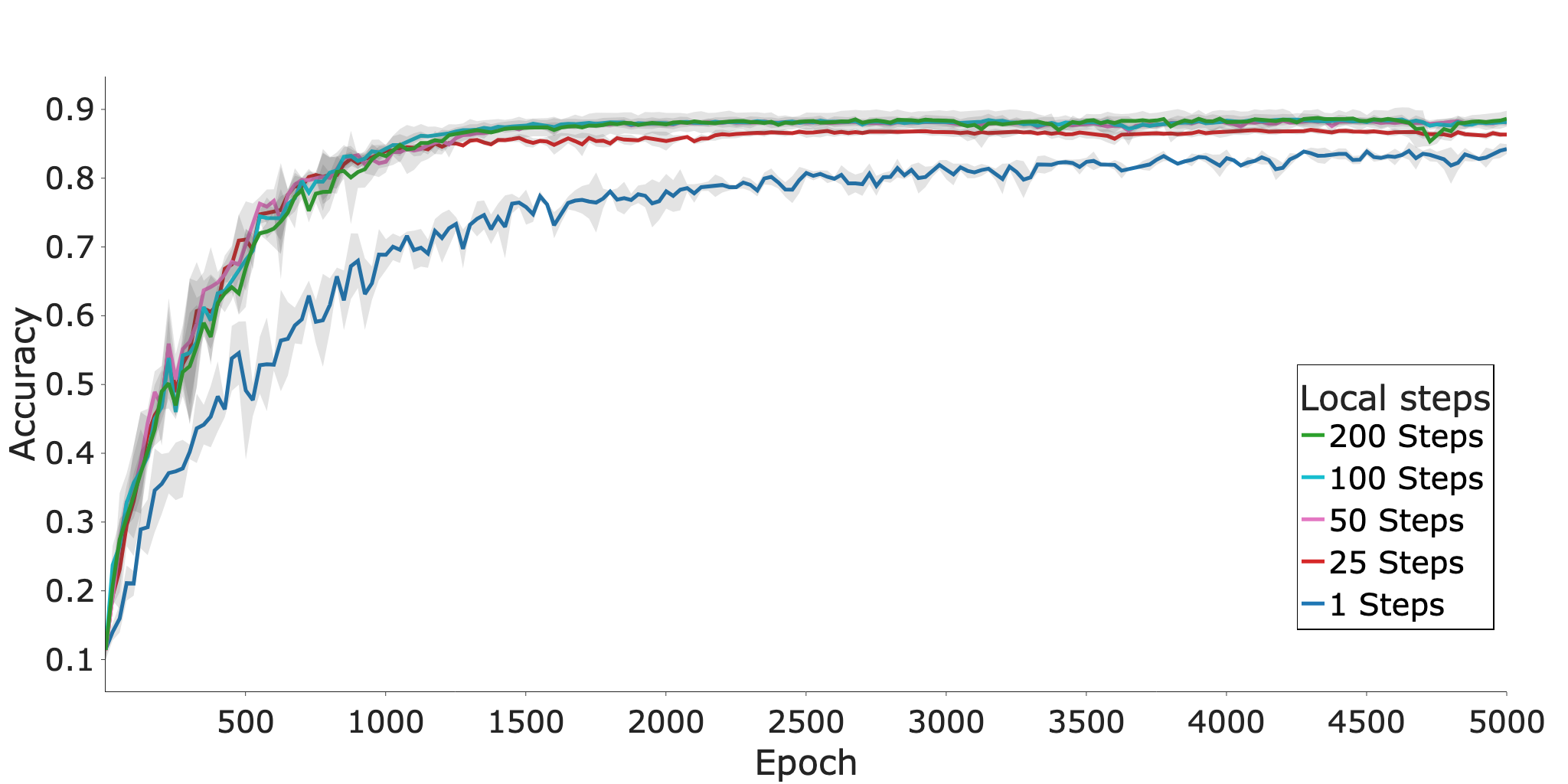
Figure 5: Effect of the number of local optimization steps on the test accuracy for the CIFAR10 dataset.

First, we examine the effect of performing local optimization step and transmitting $\Delta\theta$ back to the hypernetwork. Figure 5 shows the test accuracy throughout the training process. It compares training using the standard chain rule ($\text{steps}=1$) with the case of training locally for $k$ steps, $k\in\{25,50,100,200\}$. Using our proposed update rule, i.e., making multiple local update steps, yields large improvements in both convergence speed and final accuracy, compared to using the standard chain rule (i.e., $k=1$). The results show that pFedHN is relatively robust to the choice of local local optimization steps. As stated in the main text we set $k=50$ for all experiments.

C.2.2 Client Embedding Dimension

Next, we investigate the effect of embedding vector dimension on pFedHN performance. Specifically, we run an ablation study on set of different embedding dimensions $\{5,15,25,35\}$. The results are presented in Figure 6 (a). We show pFedHN robustness to the dimension of the client embedding vector; hence we fix the embedding dimension through all experiments to $\lfloor 1+n/4\rfloor$, where $n$ is the number of client.

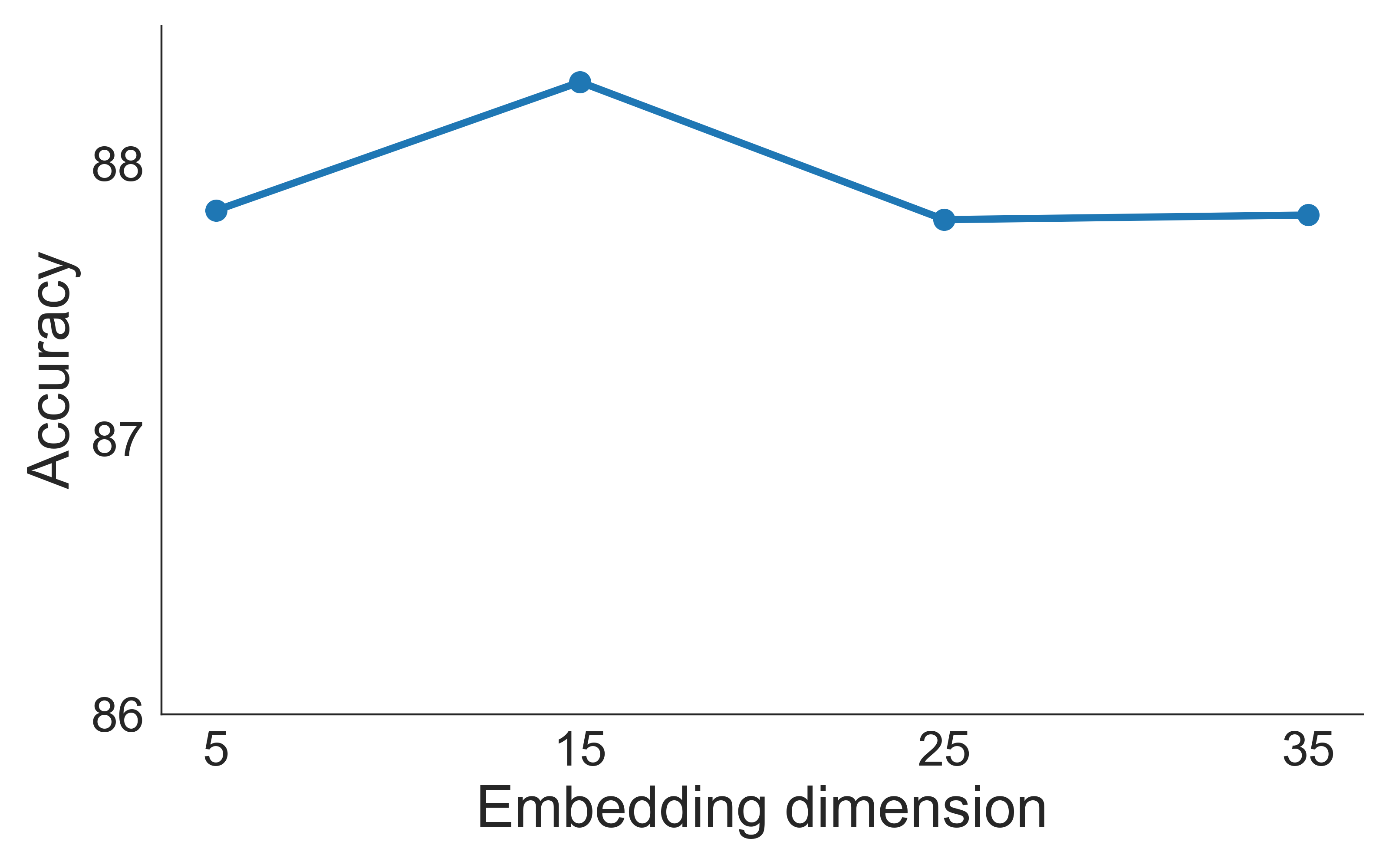
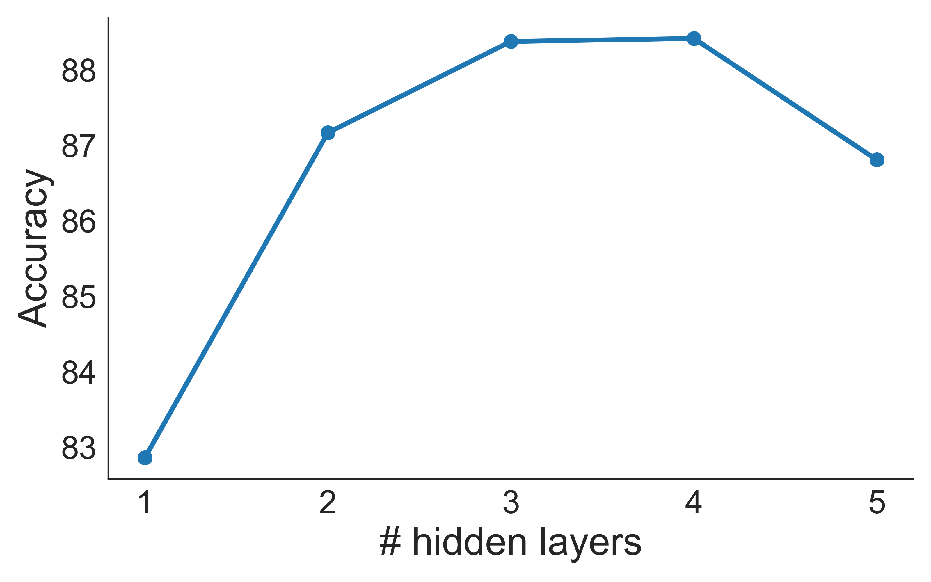
Figure 6: Test results on CIFAR10 showing the effect of (a) the dimension of the the client embedding vector, and; (b) the number of hypernetwork’s hidden layers.

C.2.3 Hypernetwork Capacity

Here we inspect the effect of the HN’s capacity on the local networks performance. We conducted an experiment in which we change the depth of the HN by stacking fully connected layers.

We evaluate pFedHN on CIFAR10 dataset using $k\in\{1,2,3,4,5\}$ hidden layers. Figure 6 (b) presents the final test accuracy. pFedHN achieves optimal performance with $k=3$ and $k=4$ hidden layers, with accuracies $88.38$ and $88.42$ respectively. We use a three hidden layers HN for all experiments in the main text.

C.3 Spectral Normalization

Table 4: pFedHN with spectral-normalization.

	CIFAR10
	10	50	100
pFedHN (ours)	$90.94\pm 2.18$	$87.02\pm 0.22$	$85.3\pm 1.81$

We show in Theorem 1 that the generalization is affected by the hypernetworks Lipschitz constant $L_{h}$. This theoretical result suggests that we can benefit from bounding this constant. Here we empirically test this by applying spectral normalization (Miyato et al., 2018) for all layers of the HN. The results are presented in Table 4. We do not observe any significant improvement compared to the results without spectral normalization (presented in Table 1 of the main text).

C.4 Generalization to Novel Clients

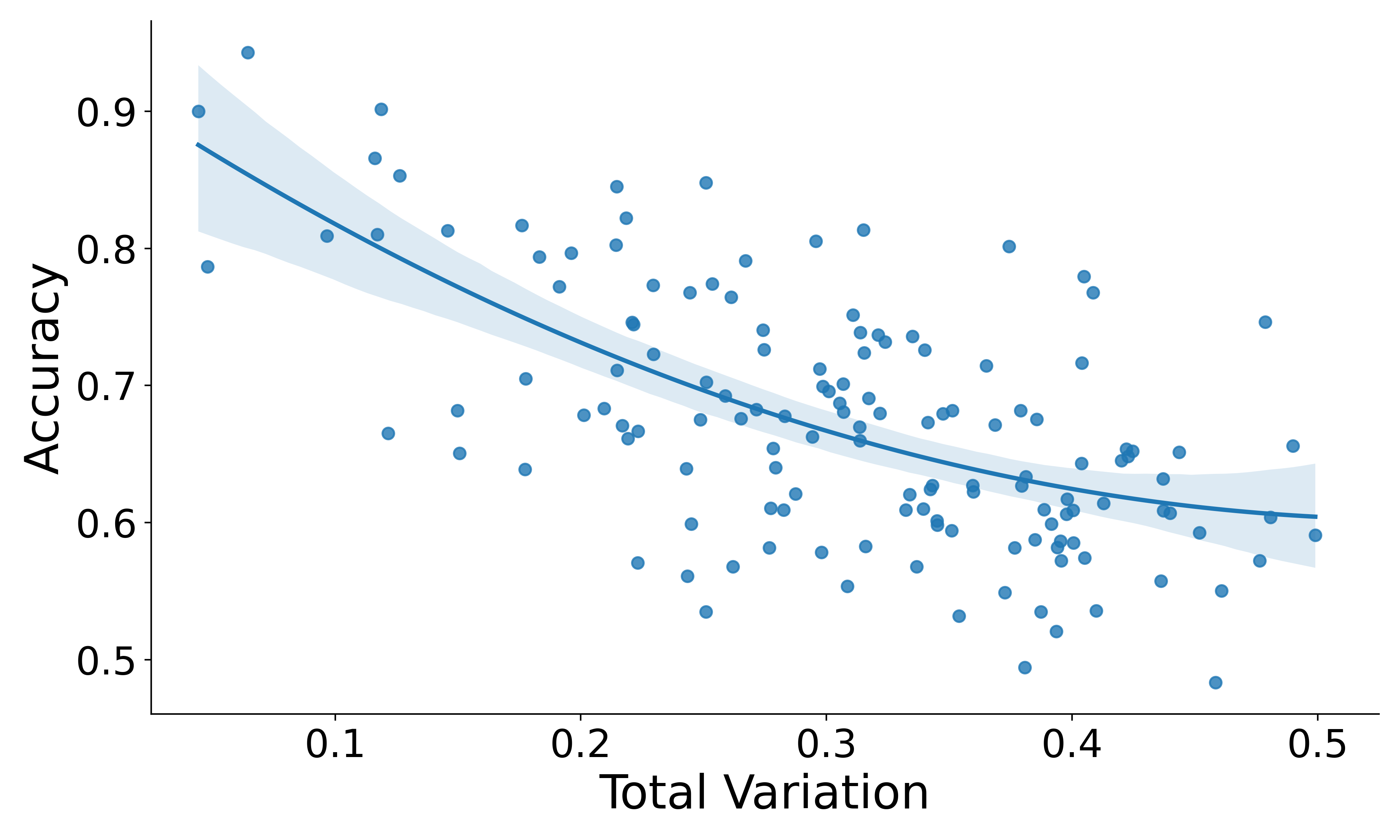
Figure 7: Accuracy for novel clients on the CIFAR10 test set. Each point represents a different client. Total variation is computed w.r.t the nearest training set client.

Here we provide additional results on the generalization performance for novel clients, studied in Section 5.3 of the main text. Figure 7 shows the accuracy of individual clients as a function of the total variation distance. Each point represents a different client, where the total variation distance is calculated w.r.t to the nearest training set client. As expected, the results show (on average) that the test accuracy decreases with the increase in the total variation distance.

C.5 Fixed Client Representation

We wish to compare the performance of pFedHN when trained with a fixed vs trainable client embedding vectors. We use CIFAR10 with the data split described in Section 5.3 of the main text and $50$ clients. We use a client embedding dimension of $10$. We set the fixed embedding vector for client $i$ to the vector of class proportions, $\hat{p}_{i}$, described in Section 5.3. pFedHN achieves similar performance with both the trainable and fixed client embedding, $84.12\pm 0.42$ and $83.92\pm 0.36$ respectively.

References

- Agarwal et al. (2018) Agarwal, N., Suresh, A. T., Yu, F. X. X., Kumar, S., and McMahan, B. cpsgd: Communication-efficient and differentially-private distributed sgd. In Advances in Neural Information Processing Systems, pp. 7564–7575, 2018.
- Arivazhagan et al. (2019) Arivazhagan, M. G., Aggarwal, V., Singh, A. K., and Choudhary, S. Federated learning with personalization layers. arXiv preprint arXiv:1912.00818, 2019.
- Bae & Grosse (2020) Bae, J. and Grosse, R. B. Delta-stn: Efficient bilevel optimization for neural networks using structured response jacobians. ArXiv, abs/2010.13514, 2020.
- Basu et al. (2020) Basu, D., Data, D., Karakus, C., and Diggavi, S. N. Qsparse-local-sgd: Distributed sgd with quantization, sparsification, and local computations. IEEE Journal on Selected Areas in Information Theory, 1(1):217–226, 2020.
- Baxter (2000) Baxter, J. A model of inductive bias learning. Journal of artificial intelligence research, 12:149–198, 2000.
- Behl et al. (2019) Behl, H. S., Baydin, A. G., and Torr, P. H. Alpha maml: Adaptive model-agnostic meta-learning. arXiv preprint arXiv:1905.07435, 2019.
- Dai et al. (2019) Dai, X., Yan, X., Zhou, K., Yang, H., Ng, K. K., Cheng, J., and Fan, Y. Hyper-sphere quantization: Communication-efficient sgd for federated learning. arXiv preprint arXiv:1911.04655, 2019.
- Deng et al. (2020) Deng, Y., Kamani, M. M., and Mahdavi, M. Adaptive personalized federated learning. arXiv preprint arXiv:2003.13461, 2020.
- Dinh et al. (2020) Dinh, C. T., Tran, N. H., and Nguyen, T. D. Personalized federated learning with moreau envelopes. ArXiv, abs/2006.08848, 2020.
- Duchi et al. (2014) Duchi, J. C., Jordan, M. I., and Wainwright, M. J. Privacy aware learning. Journal of the ACM (JACM), 61(6):1–57, 2014.
- Fallah et al. (2020a) Fallah, A., Mokhtari, A., and Ozdaglar, A. Personalized federated learning: A meta-learning approach. ArXiv, abs/2002.07948, 2020a.
- Fallah et al. (2020b) Fallah, A., Mokhtari, A., and Ozdaglar, A. On the convergence theory of gradient-based model-agnostic meta-learning algorithms. In International Conference on Artificial Intelligence and Statistics, pp. 1082–1092. PMLR, 2020b.
- Finn et al. (2017) Finn, C., Abbeel, P., and Levine, S. Model-agnostic meta-learning for fast adaptation of deep networks. arXiv preprint arXiv:1703.03400, 2017.
- Ha et al. (2017) Ha, D., Dai, A. M., and Le, Q. V. Hypernetworks. ArXiv, abs/1609.09106, 2017.
- Haddadpour & Mahdavi (2019) Haddadpour, F. and Mahdavi, M. On the convergence of local descent methods in federated learning. arXiv preprint arXiv:1910.14425, 2019.
- Hanzely & Richtárik (2020) Hanzely, F. and Richtárik, P. Federated learning of a mixture of global and local models. arXiv preprint arXiv:2002.05516, 2020.
- Hsu et al. (2019) Hsu, T. H., Qi, H., and Brown, M. Measuring the effects of non-identical data distribution for federated visual classification. ArXiv, abs/1909.06335, 2019.
- Huang et al. (2020) Huang, Y., Chu, L., Zhou, Z., Wang, L., Liu, J., Pei, J., and Zhang, Y. Personalized cross-silo federated learning on non-iid data. 2020.
- Huo et al. (2020) Huo, Z., Yang, Q., Gu, B., Huang, L. C., et al. Faster on-device training using new federated momentum algorithm. arXiv preprint arXiv:2002.02090, 2020.
- Kairouz et al. (2019) Kairouz, P., McMahan, H. B., Avent, B., Bellet, A., Bennis, M., Bhagoji, A. N., Bonawitz, K., Charles, Z., Cormode, G., Cummings, R., et al. Advances and open problems in federated learning. arXiv preprint arXiv:1912.04977, 2019.
- Karimireddy et al. (2019) Karimireddy, S. P., Kale, S., Mohri, M., Reddi, S. J., Stich, S. U., and Suresh, A. T. Scaffold: Stochastic controlled averaging for on-device federated learning. arXiv preprint arXiv:1910.06378, 2019.
- Klein et al. (2015) Klein, B., Wolf, L., and Afek, Y. A dynamic convolutional layer for short rangeweather prediction. 2015 IEEE Conference on Computer Vision and Pattern Recognition (CVPR), pp. 4840–4848, 2015.
- Klocek et al. (2019) Klocek, S., Maziarka, Ł., Wołczyk, M., Tabor, J., Nowak, J., and Śmieja, M. Hypernetwork functional image representation. In International Conference on Artificial Neural Networks, pp. 496–510. Springer, 2019.
- Krizhevsky & Hinton (2009) Krizhevsky, A. and Hinton, G. Learning multiple layers of features from tiny images. Technical report, University of Toronto, 2009.
- Kulkarni et al. (2020) Kulkarni, V., Kulkarni, M., and Pant, A. Survey of personalization techniques for federated learning. 2020 Fourth World Conference on Smart Trends in Systems, Security and Sustainability (WorldS4), pp. 794–797, 2020.
- Lake et al. (2015) Lake, B. M., Salakhutdinov, R., and Tenenbaum, J. B. Human-level concept learning through probabilistic program induction. Science, 350(6266):1332–1338, 2015.
- LeCun et al. (1998) LeCun, Y., Bottou, L., Bengio, Y., and Haffner, P. Gradient-based learning applied to document recognition. Proceedings of the IEEE, 86(11):2278–2324, 1998.
- Li et al. (2019) Li, Q., Wen, Z., and He, B. Federated learning systems: Vision, hype and reality for data privacy and protection. ArXiv, abs/1907.09693, 2019.
- Li et al. (2020a) Li, T., Sahu, A. K., Talwalkar, A., and Smith, V. Federated learning: Challenges, methods, and future directions. IEEE Signal Processing Magazine, 37(3):50–60, 2020a.
- Li et al. (2017) Li, Z., Zhou, F., Chen, F., and Li, H. Meta-sgd: Learning to learn quickly for few-shot learning. arXiv preprint arXiv:1707.09835, 2017.
- Li et al. (2020b) Li, Z., Kovalev, D., Qian, X., and Richtárik, P. Acceleration for compressed gradient descent in distributed and federated optimization. arXiv preprint arXiv:2002.11364, 2020b.
- Liang et al. (2020) Liang, P. P., Liu, T., Ziyin, L., Allen, N. B., Auerbach, R. P., Brent, D., Salakhutdinov, R., and Morency, L.-P. Think locally, act globally: Federated learning with local and global representations. arXiv preprint arXiv:2001.01523, 2020.
- Lin et al. (2018) Lin, T., Stich, S. U., Patel, K. K., and Jaggi, M. Don’t use large mini-batches, use local sgd. arXiv preprint arXiv:1808.07217, 2018.
- Lorraine & Duvenaud (2018) Lorraine, J. and Duvenaud, D. Stochastic hyperparameter optimization through hypernetworks. ArXiv, abs/1802.09419, 2018.
- Maaten & Hinton (2008) Maaten, L. V. D. and Hinton, G. E. Visualizing data using t-sne. Journal of Machine Learning Research, 9:2579–2605, 2008.
- MacKay et al. (2019) MacKay, M., Vicol, P., Lorraine, J., Duvenaud, D., and Grosse, R. B. Self-tuning networks: Bilevel optimization of hyperparameters using structured best-response functions. ArXiv, abs/1903.03088, 2019.
- Mansour et al. (2020) Mansour, Y., Mohri, M., Ro, J., and Suresh, A. T. Three approaches for personalization with applications to federated learning. ArXiv, abs/2002.10619, 2020.
- McMahan et al. (2017a) McMahan, H., Moore, E., Ramage, D., Hampson, S., and y Arcas, B. A. Communication-efficient learning of deep networks from decentralized data. In AISTATS, 2017a.
- McMahan et al. (2017b) McMahan, H. B., Ramage, D., Talwar, K., and Zhang, L. Learning differentially private recurrent language models. arXiv preprint arXiv:1710.06963, 2017b.
- Miyato et al. (2018) Miyato, T., Kataoka, T., Koyama, M., and Yoshida, Y. Spectral normalization for generative adversarial networks. In International Conference on Learning Representations, ICLR, 2018.
- Mothukuri et al. (2021) Mothukuri, V., Parizi, R. M., Pouriyeh, S., Huang, Y., Dehghantanha, A., and Srivastava, G. A survey on security and privacy of federated learning. Future Generation Computer Systems, 115:619–640, 2021.
- Muresan & Parks (2003) Muresan, D. D. and Parks, T. W. Adaptive principal components and image denoising. In Proceedings 2003 International Conference on Image Processing (Cat. No.03CH37429), 2003.
- Nachmani & Wolf (2019) Nachmani, E. and Wolf, L. Hyper-graph-network decoders for block codes. In Wallach, H. M., Larochelle, H., Beygelzimer, A., d’Alché-Buc, F., Fox, E. B., and Garnett, R. (eds.), Advances in Neural Information Processing Systems 32: Annual Conference on Neural Information Processing Systems 2019, NeurIPS 2019, December 8-14, 2019, Vancouver, BC, Canada, pp. 2326–2336, 2019. URL https://proceedings.neurips.cc/paper/2019/hash/a9be4c2a4041cadbf9d61ae16dd1389e-Abstract.html.
- Navon et al. (2021) Navon, A., Shamsian, A., Chechik, G., and Fetaya, E. Learning the pareto front with hypernetworks. In International Conference on Learning Representations, 2021. URL https://openreview.net/forum?id=NjF772F4ZZR.
- Nichol et al. (2018) Nichol, A., Achiam, J., and Schulman, J. On first-order meta-learning algorithms. arXiv preprint arXiv:1803.02999, 2018.
- Reisizadeh et al. (2020) Reisizadeh, A., Mokhtari, A., Hassani, H., Jadbabaie, A., and Pedarsani, R. Fedpaq: A communication-efficient federated learning method with periodic averaging and quantization. In International Conference on Artificial Intelligence and Statistics, pp. 2021–2031. PMLR, 2020.
- Riegler et al. (2015) Riegler, G., Schulter, S., Rüther, M., and Bischof, H. Conditioned regression models for non-blind single image super-resolution. 2015 IEEE International Conference on Computer Vision (ICCV), pp. 522–530, 2015.
- Sahu et al. (2018) Sahu, A. K., Li, T., Sanjabi, M., Zaheer, M., Talwalkar, A., and Smith, V. On the convergence of federated optimization in heterogeneous networks. arXiv preprint arXiv:1812.06127, 3, 2018.
- Smith et al. (2017) Smith, V., Chiang, C.-K., Sanjabi, M., and Talwalkar, A. S. Federated multi-task learning. In Advances in neural information processing systems, pp. 4424–4434, 2017.
- Stich (2018) Stich, S. U. Local sgd converges fast and communicates little. arXiv preprint arXiv:1805.09767, 2018.
- Suarez (2017) Suarez, J. Character-level language modeling with recurrent highway hypernetworks. In Proceedings of the 31st International Conference on Neural Information Processing Systems, pp. 3269–3278, 2017.
- von Oswald et al. (2019) von Oswald, J., Henning, C., Sacramento, J., and Grewe, B. F. Continual learning with hypernetworks. arXiv preprint arXiv:1906.00695, 2019.
- Wang & Joshi (2018) Wang, J. and Joshi, G. Cooperative sgd: A unified framework for the design and analysis of communication-efficient sgd algorithms. arXiv preprint arXiv:1808.07576, 2018.
- White (1982) White, H. Maximum likelihood estimation of misspecified models. Econometrica, 50:1–25, 1982.
- Wu et al. (2020) Wu, Q., He, K., and Chen, X. Personalized federated learning for intelligent iot applications: A cloud-edge based framework. IEEE Open Journal of the Computer Society, 1:35–44, 2020.
- Yang et al. (2019) Yang, Q., Liu, Y., Chen, T., and Tong, Y. Federated machine learning: Concept and applications. arXiv: Artificial Intelligence, 2019.
- Zhang et al. (2019) Zhang, M., Lucas, J., Ba, J., and Hinton, G. E. Lookahead optimizer: k steps forward, 1 step back. Advances in Neural Information Processing Systems, 32:9597–9608, 2019.
- Zhang et al. (2020) Zhang, M., Sapra, K., Fidler, S., Yeung, S., and Alvarez, J. M. Personalized federated learning with first order model optimization. arXiv preprint arXiv:2012.08565, 2020.
- Zhao et al. (2018) Zhao, Y., Li, M., Lai, L., Suda, N., Civin, D., and Chandra, V. Federated learning with non-iid data. arXiv preprint arXiv:1806.00582, 2018.
- Zhou & Cong (2017) Zhou, F. and Cong, G. On the convergence properties of a -step averaging stochastic gradient descent algorithm for nonconvex optimization. arXiv preprint arXiv:1708.01012, 2017.
- Zhou et al. (2019) Zhou, P., Yuan, X., Xu, H., Yan, S., and Feng, J. Efficient meta learning via minibatch proximal update. Advances in Neural Information Processing Systems, 32:1534–1544, 2019.
- Zhu et al. (2019) Zhu, W., Kairouz, P., Sun, H., McMahan, B., and Li, W. Federated heavy hitters discovery with differential privacy. arXiv preprint arXiv:1902.08534, 2019.