Comparing Popular Simulation Environments in the Scope of Robotics and Reinforcement Learning

Abstract

This letter compares the performance of four different, popular simulation environments for robotics and reinforcement learning (RL) through a series of benchmarks. The benchmarked scenarios are designed carefully with current industrial applications in mind. Given the need to run simulations as fast as possible to reduce the real-world training time of the RL agents, the comparison includes not only different simulation environments but also different hardware configurations, ranging from an entry-level notebook up to a dual CPU high performance server. We show that the chosen simulation environments benefit the most from single core performance. Yet, using a multi core system, multiple simulations could be run in parallel to increase the performance.

I Introduction

In the last years, simulations became an ever more important part of hardware development, especially in the field of robotics and reinforcement learning (RL) [1, 2]. Modern RL methods show incredible results with virtual humanoid models learning to walk, robots learning to grip and throw different objects, to name a few [3, 4, 5]. Many of these use cases describe theoretical fields of application and are not yet used in a value adding environment. In fact, however, the RL methodology has great advantages in the field of industrial production automation. Especially the task of automated process control can benefit from the versatility and flexibility of an RL agent, mostly because current process flows in industrial environments are based on fixed programmed algorithms, offering limited flexibility to react to changed process states. In particular for complex processes, fixed programmed algorithms quickly reach the limits of their capabilities simply because the integration of experience into classic code is often only possible to a restricted extent. RL has the ability to learn from experiences and apply the learned knowledge to real production processes. Similar to other machine learning applications, the acquisition of training data is one of the more challenging tasks. The quality of training data closely correlates to the quality of the simulation environment generating this data. Thus, the quantity of the training data depends on the speed of the simulation environment.

Therefore, developers need a reliable simulation environment with a physical model which represents their process environment well enough to produce meaningful data [6]. Throughout the years, a large number of physics-based simulation environments that meet those requirements has been developed. Especially developers of automation applications or scientists who have no previous experience with simulation environments and physic engines find it difficult to choose the right environments for their projects.

The goal of this work is to facilitate the selection of simulation environments by presenting evaluations of simulation stability, speed, and hardware utilization for four simulation environments which are widely used in the research community. The focus of the investigations is placed on the realization of RL applications. This also means that, in comparison to the classical development of algorithms, minor inaccuracies in the calculation of physical effects can be tolerated. Advantages as well as disadvantages will be highlighted which help to emphasize the applicability of the selected simulation environments in the industrial context. More precisely, criteria such as usability, model creation and parameter setup have been evaluated. All the APIs used for this work are Python-based.

In addition, a statement is made regarding which of the selected tools can be used to create a stable simulation most quickly and easily by an inexperienced user. However, as there is no one-fits-all solution, we cannot give a single, universal recommendation about which simulation environment to use. Instead, this paper is intended to facilitate the selection of RL methods especially for scientists and developers with little previous experience in this field.

From the beginning, the authors had basic experiences with diverse simulation environments which are described in section IV. During the development of the benchmark, they intensively worked with each of the four simulation environments considered in this work. This has resulted in a profound knowledge of the simulation applications even though it cannot be equated with the knowledge of a long-standing expert. We are aware that the results and estimates for individual simulation environments could be refined and optimized by such an expert. However, the data and analyses of this work correspond better to the working reality of beginners or advanced users of the considered simulation environments. The individual simulation environments use existing or customized physic engines to calculate the behavior of bodies with mass under the influence of forces such as gravity, inertia or contact constraints. In this work, we focus on the applicability of the simulation tool but not on the accuracy of the physic engines since this represents a separate field of research. None of the authors has any business or financial ties to the developers or companies of the simulation environments discussed here. A detailed description of the scenarios, parameters and settings used can be found at https://github.com/zal/simenvbenchmark.

II Related work

With the increasing popularity of RL applications, several papers have focused on the capabilities and functions of physics engines. The emphasis of our work is on different aspects.

Ayala et al. [7] focused on a quantitative, hardware load specific comparison of Webots, Gazebo and V-Rep. They were using the humanoid robot NAO running around a chair controlled by an external controller. The work evaluated the system load of each simulation environment on one low-end PC system without comparing it to the real-time factor ($RTF$).

Pitonakova et al. [8] compared Gazebo, V-Rep and ARGoS for their functionalities and simulation speed. Their work focuses on the development of mobile robot controls. Therefore, two model scenes were used to perform the benchmarks in GUI and headless mode. The evaluation includes the $RTF$, CPU and memory utilization. They were able show that Gazebo is faster for larger model scenes whereas ARGoS is able to simulate a higher number of robots in smaller scenes. Unfortunately, the used benchmark models are not identical from simulator to simulator. Instead, mainly already existing models from the internal libraries are used which differ from each other, making the objective comparison more difficult.

The developers of MuJoCo describe a slightly different approach compared to the work mentioned above [9]. They compare abstract, dynamic application scenarios, based on physical engines (Bullet, Havok, MuJoCo, ODE, and PhysX) on which the simulation environments are based on. These engines are being evaluated in terms of simulation stability and speed by increasing the time step after each run. Thus, it is possible to determine at which time steps errors occurred compared to the runs at the lowest time step. Such a measure is, in general, a good approximation at which time step the simulation becomes unstable. These findings rate MuJoCo as the most accurate and fastest physic engine regarding robotic applications. The other engines show their potential in game scenarios and multi-body models with unconnected elements.

III Objectives of the Benchmark

Given our need for a fast, yet stable and precise simulation environment, we decided to build two scenarios. The first scenario is closely related to our use case, simulating industrial robots. Thus, we build the scenario around the Universal Robot UR10e equipped with the Robotiq 3-Finger Gripper, a commonly used robot and endeffector, for example in [10]. In this scenario the robot was given the task to rearrange and stack small cylinders, as seen in Fig. 1. To achieve the task, the robot, especially the complex gripper, has to perform small and precise movements. Likewise, the simulation environment has to be precise for the task not to fail.

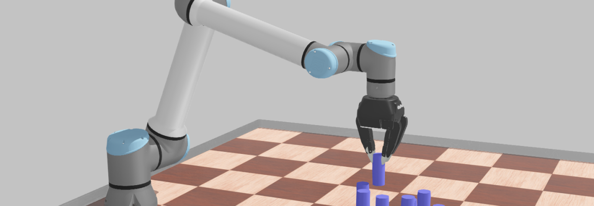
Figure 1: The first scenario with the robot and the cylinders in Webots.

However, this scenario is characterized by a low number of simultaneous contacts. As many scenarios, especially in industrial applications, consist of multi-body-collisions, such as a robot sorting through a bin of objects, we designed a second benchmark scenario. The second rather generic scenario is built around a multitude of spheres. Those are arranged in a cube with side length of $6$ spheres, see Fig. 2, a total of $216$ densely packed spheres, all falling down at the same time and then spreading frictionless on the floor, generating a higher number of simultaneous contacts.

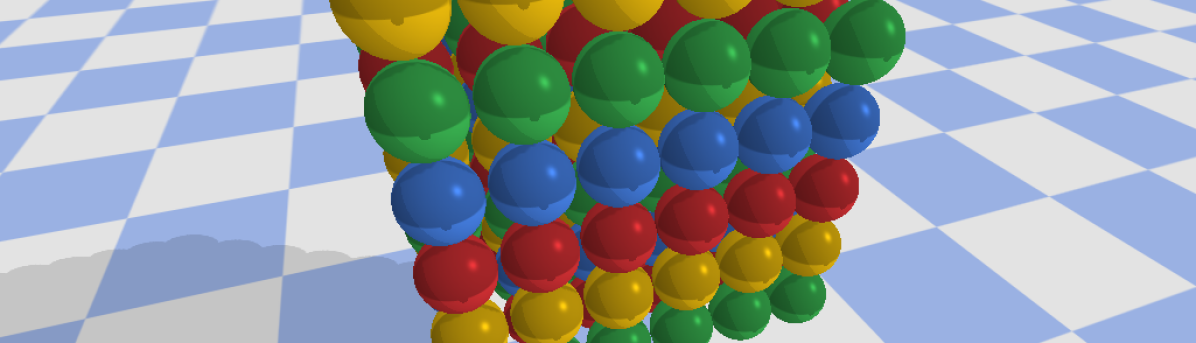
Figure 2: The second scenario with a cube build from spheres in PyBullet.

IV Considered Simulation Environments

Among the most popular rigid body simulation environments for robotics and RL are Gazebo, MuJoCo, PyBullet, and Webots [1, 11]. However, while each physics engine is designed to portray the real world in a general way, each implementation has its own strengths and caveats [12].

In contrast to simulations used in finite element method (FEM) and computational fluid dynamics (CFD), which can take hours or days for a single simulation step, robotic and RL applications require a responsive simulation environment running at least at real-time. Responsiveness can be achieved when the $RTF$, the ratio of simulation time over real-world time, is at least around $1$. Furthermore, especially RL greatly benefits from a $RTF$ of above $1$, as the agent can now be trained faster than in real-time leading to lower waiting times for the training. Hence, while pure robotic simulations like a digital-twin in general do not benefit from an $RTF$ above $1$, RL does. Nevertheless, higher real-time factors always come with lower precision as we will show in section VIII. Thus, as FEM and CFD need to be as precise as possible, they are accordingly slow. Robotic and RL application in most cases do not need such precision and can thus use simulation environments with reduced precision in favor of speed. A simple and often used way to increase the speed is by increasing the time step of the simulation, simultaneously reducing the precision. However, the precision needs to be good enough, meaning the simulation must portray the real world physics good enough for the individual use case to work. In the presented scenario regarding the UR10e with Robotiq 3-Finger Gripper, all simulators, apart from Gazebo, used a joint position controller. Since the existing repositories for Gazebo used an joint trajectory controller with effort interface, we chose to use it as well. For this, the PID values had to be tuned, which introduced an additional source of error.

IV-A Gazebo

Gazebo is a open-source robotics simulation environment and supports four physics engines: Bullet [13], Dynamic Animation and Robotics Toolkit (DART) [14], Open Dynamics Engine (ODE) [15] and Simbody [16]. The development started in 2002 at the University of Southern California as a stand-alone simulator and was expanded in 2009 with an integration of an interface for the Robot Operating System (ROS). Since the foundation of the Open Source Robotics Foundation (OSRF) [17] in 2012, OSRF has been leading the development and is supported by a large community [18].

IV-B MuJoCo

MuJoCo (Multi-Joint dynamics with Contact) is a simulation environment and physic engine focused on robotic and biomechanic simulation, as well as animation and machine learning application [19]. It is commonly known for RL applications that train an agent to enable virtual animal or humanoid models to walk or perform other complex actions [20]. MuJoCo provides a native, XML-based model description format which is designed to be human readable and editable. In contrast to the other simulation environments described in this work, a license is required to be able to install it. However, not all licenses allow the usage of MuJoCo inside a Docker container. Only an academic license allows using MuJoCo inside a Docker container which we were not able to acquire.

IV-C PyBullet

The simulation environment PyBullet is based on the Bullet physics-based simulation environment. It focuses on machine learning applications in combination with robotic applications [21]. PyBullet is characterized in particular by a large community [22] which further develops this simulation environment as an open-source project and offers support for beginners. In addition, the import of robot and machinery models is simplified as a wide variety of model formats can be loaded, such as SDF, URDF and MJCF (MuJoCo’s model format).

IV-D Webots

Webots is an open source and multi-platform desktop application used to simulate robots. It provides a complete development environment to model, program and simulate robots [23]. Webots offers an extensive library of sample worlds, sensors and robot models. Robots may be programmed in C, C++, Python, Java, MATLAB or ROS, with detailed API documentation for each option. Models can be imported from multiple CAD formats or converted from URDF. At its core, Webots uses a customized ODE physics engine.

V Benchmark Scenarios

As already mentioned in section III, we defined two scenarios for this benchmark. The first benchmark is built around the Universal Robot UR10e robot equipped with the Robotiq 3-Finger Gripper. It is commonly used in industrial applications, especially for grasping tasks [10, 24]. In this scenario, we model the grasping task by rearranging and stacking multiple cylinders, as shown in Fig. 1. In total, there are $21$ cylinders, of which the robot directly interacts with $9$ cylinders by gripping those. The first task of the robot is to stack one cylinder on top of another $8$ times along a circle. Afterwards, the robot builds a tower of $7$ cylinders, the maximum it can stack whilst facing the hand downwards. The duration of the trajectory is $279\text{\,}\mathrm{s}$. This scenario requires precise control of the UR10e and the gripper. The cylinders positions were chosen so that slight deviations of the position will knock over other cylinders. Moreover, if the grippers were unable to apply sufficient force to the cylinders they would slip and the task would fail. All those precise movements require the simulation environments to accurately calculate not only the state of the system but also the contacts between the objects.

The second scenario is characterized by the increased number of simultaneous contacts that occur especially at the beginning of the benchmark. Here, multiple spheres are ordered in a cubical grid with side length of six spheres, see Fig. 2. Once falling down, all those $216$ spheres will interact with each other and start spreading frictionless on the ground floor. Due to the slight perturbations, which are the same for all simulations, in the initial position of the spheres along the grid the spheres spread randomly as opposed to a symmetrical spreading along the floor plane. After $4\text{\,}\mathrm{s}$, the spheres are mostly moving freely on the ground plate and the simulation is stopped. As the aforementioned perturbations introduce chaos, we cannot clearly define the desired position for the spheres at any time past the moment, the spheres come into contact with one another. However, we can deduct if the spreading pattern itself is deterministic given a simulation environment and a time step. Thus, allowing us to qualitatively analyze the movement of the spheres and moreover determine the $RTF$ with respect to the number of theoretically contact, see section VIII.

VI Software Framework

Each simulation environment has a specific controller, providing methods to change physics parameters, communicate with robot controllers and retrieve simulation data. The core of our software framework is a Python script, referred to as taskEnv, identical for each simulation environment with three main functions. First, change the time step of the connected simulation. Secondly, send identical control commands given the predefined trajectory. And thirdly, retrieve data from the simulation and generate a log. A shell script launches the hardware monitor and each simulation environment executes the taskEnv for the specified time steps. For the spheres scenario, the structure is virtually the same, with the difference of no trajectory control commands being transmitted.

VI-A Real-Time Factor Calculation

The real-time factor $RTF$ was calculated using $RTF=\Delta t_{\mathrm{sim}}\cdot\Delta t_{\mathrm{real}}^{-1}$, were $\Delta t_{\mathrm{sim}}$ is the duration of the current time step and $\Delta t_{\mathrm{real}}$ the time it took the system to calculate the respective time step. The total $RTF$ of one simulation run was then calculated as the average of all its $RTF$s. In MuJoCo, PyBullet and Webots, rather than continuously executing the simulation, each simulation step has to be explicitly called through the API. For these simulation environments $\Delta t_{\mathrm{real}}$ was calculated by taking a time stamp before and after each simulation step call using Python’s time.perf_counter(). For the average $RTF$ of a benchmark run the final $t_{\mathrm{sim}}$ was divided by the sum of all $\Delta t_{\mathrm{real}}$.

Since we wanted to rely on the existing Phyton APIs and did not want to write any further plugins, we had to use the existing control mechanisms, such as the ROS API for Gazebo, namely rospy. While Gazebo also allows to call each step explicitly, rospy does not. Therefore, Gazebo runs continuously and the $RTF$ was calculated by taking a timestamp at the start and end of a benchmark run. Simulation time $t_{\mathrm{sim}}$ was retrieved by subscribing to the ROS topic /clock. This may lead to inaccurate results for the significantly shorter sphere scenario which only lasts for four simulation seconds, especially for higher time steps. Furthermore, it should be noted that our $RTF$ values do not necessarily represent the $RTF$ values displayed by the GUIs of each simulation environment as different formulas might be used.

VII Benchmark Procedure

As discussed before, the speed of the simulation environment is heavily dependent on the time step. The same applies to precision, but anti-proportional. Thus, we ran the benchmark for different time steps, evaluating the performance and, in the case of the robot scenario, also the precision. In our setup, the time steps range from $1\text{\,}\mathrm{ms}64\text{\,}\mathrm{ms}$, starting in steps of $1\text{\,}\mathrm{ms}$. Moreover, in order to gain statistical significance, we ran each time step $5$ times per scenario, environment and hardware configuration. Furthermore, we ensured the CPU cooled down again after every run to not run into thermal throttling which could reduce the performance and influence the results for subsequent simulation environments. This way, we wanted to ensure that we did not bias the results given the order we ran the benchmarks.

VII-A Hardware Systems Used for Benchmark Run

To reflect the wide variety of possible systems used to compute the simulations, multiple target systems were defined. The configuration was chosen to reflect typical systems available in research for simulating and training an environment. Thus, the configurations range from an entry-level notebook with only an Intel iGPU to a rendering/simulation server, which might be available at an institution or can be rented at Amazon AWS or Microsoft Azure. The technical specifications are listed in table I.

TABLE I: Hardware Systems

	CPU	GPU	RAM	Storage
Server	$$2$\times$ AMD EPYC 7542	$$4$\times$ NVIDIA Quadro RTX 8000	$512\text{\,}\mathrm{GiB}$ DDR4	Samsung PM1733
Mobile workstation	Intel Core i7-8700	NVIDIA GeForce RTX 2080 Mobile	$32\text{\,}\mathrm{GiB}$ DDR4	Samsung 960 EVO
Notebook	Intel Core i7-7500U	Intel HD Graphics 620	$8\text{\,}\mathrm{GiB}$ DDR4	Samsung 950 Pro

All systems were up-to-date as of the date of the benchmarks with the host OS being Ubuntu 20.04.1 LTS with kernel 5.4.0-52-generic, Docker version 19.03.13 (build 4484c46d9d), Python 3.8.2, and ROS Noetic Ninjemys. The systems with an NVIDIA GPU both used driver version 455.23.04 coupled with CUDA 11.1, as well as NVIDIA-Docker version 2.5.0-1 to enable GPU pass-through. The simulation environments were running versions 11.1.0 for Gazebo, 200 for MuJoCo, 2.8.4 for PyBullet, and R2020b-rev1 for Webots.

While a GUI is important for developing the scenario in every simulator, we chose to run the simulations ”headless”, i.e. no GUI was spawned. This decision was based on the fact that many servers applications are running headless. Running the simulation environments headless is a built-in option for Gazebo, MuJoCo and PyBullet. Only Webots does not currently offer support for running headless. However, it provides a mode called ”fast”, which does not render any visualisation while still spawning a GUI. Therefore, we used Xvfb (X Window Virtual Framebuffer) which creates a virtual X-server entirely on the CPU for the Webots GUI to attach to. But as the GUI is not rendering anything, this does not affect the performance.

VII-B Hardware Load Acquisition

One of the main aspects of a high performance simulation is to what extent the simulation environment itself is able to utilize the hardware resources. Therefore, the hardware load is monitored during every simulation run. To prevent the monitoring process from affecting the simulation performance, the software collectl [25] is used in a separate thread. It is able to collect a wide variety of system data. In this work we will put focus on the CPU load to give an idea how big the hardware requirements of each simulation environments are.

VII-C Container-based Software Deployment

As the goal of this paper is to run the benchmark on as many different systems as possible, we chose Docker due to its easy portability. The usage of Docker enables two important use cases for this benchmark. Firstly, it lets us create an easy to deploy image with all necessary software already installed which also runs the full benchmark setup upon starting the container. Secondly, due to Docker’s nature of userspace isolation [26], we create a clean environment for our simulations as well as the hardware load acquisition to run. According to multiple studies [27, 28, 29, 30], the performance loss of Docker is negligible, especially for CPU, GPU and RAM access. Despite the clear advantage of using Docker, we were not able to use MuJoCo inside the Docker container due to licensing problems, see section IV-B.

VIII Simulation and Results

VIII-A Simulation Stability and Performance

Based on the data evaluation, the following describes which $RTF$ is achieved during the calculation of the two use cases. Fig. 3 shows the logarithmic progression of the $RTF$s over the also logarithmic increase of time steps for the robot scenario. The data indicates that the $RTF$s have a linear gradient over the time step. However, it should be noted that the simulation does not provide valid results over the entire time step progression. Due to the increasing time steps, errors occur during the physic calculations which are reflected in an incorrect reaction of the robot or the objects. We consider a simulation result as invalid if the deviation of a observed cylinder position compared to its target position is larger than $1\text{\,}\mathrm{cm}$ as this would indicate it has slipped or fallen. Based on the solver parameters described in this thesis Webots achieves a valid simulation result up to a time step of $48\text{\,}\mathrm{ms}$. MuJoCo achieves valid results up to 3ms and PyBullet up to $7\text{\,}\mathrm{ms}$. In the latter simulation environment, however, an outlier can be observed, since at 4ms a non-valid result is obtained. Apparently, the stacked tower collapses shortly before the end of the simulation. In Gazebo all time steps are calculated, but the control of the Robotiq 3-Finger Gripper did not succeed to stabilize at time steps starting at $2\text{\,}\mathrm{ms}$. Thus, Gazebo can only generate a valid result with time steps of $1\text{\,}\mathrm{ms}$ for the use cases discuss in this work.

Figure 3: Progression of the $RTF$ for the robot scenario over increasing time steps running on the workstation.

Fig. 4 describes the same progression as Fig. 3 but for the sphere scenario. Please note that Gazebo did not generate any observations for $64\text{\,}\mathrm{ms}$. For lower time steps, the same linear trend can be observed, but with a lower initial $RTF$ due to the increased number of contacts. Nevertheless, for higher time steps the stability of the simulation environments is not guaranteed leading to a break of the trend. In an in-depth analysis of the $RTF$ over the simulation time, we discovered that the $RTF$ is greater than the average $RTF$ at the beginning. As soon as the the spheres come into contact, the $RTF$ drops significantly, only to recover and flatten out once the spheres are distributed along the ground floor and interactions are rare.

Figure 4: Progression of the $RTF$ for the sphere scenario over increasing time steps running on the workstation.

VIII-B Hardware Load

The physics engines of the simulation environments are all designed to run only on the CPU. Except for Gazebo and Webots, no multi-threaded physics calculations are provided [31, 32]. Thus, MuJoCo and PyBullet always only utilized a single core while Webots and especially Gazebo both can span specific tasks of their workload over multiple threads. Due to the comparability and the non-replicable simulations results [23], multi-threading functionalities are deactivated. Therefore, we expected all simulation environment to only utilize one core up to $100\text{\,}\mathrm{\char 37\relax}$, especially because the simulation environments are set up to run headless with maximum $RTF$ possible.

TABLE II: Average CPU Usage per Simulation Environment Compared to the Average Real-Time Factor $RTF$ with a time step of $1\text{\,}\mathrm{ms}$.

		Server		Mobile workstation		Notebook
		CPU	$RTF$	CPU	$RTF$	CPU	$RTF$
Gazebo	robot	$273.0\text{\,}\mathrm{\char 37\relax}$	$4.3$	$264.4\text{\,}\mathrm{\char 37\relax}$	$4.4$	$($11.9\text{\,}\mathrm{\char 37\relax}$)$	$2.3$
	spheres	$223.1\text{\,}\mathrm{\char 37\relax}$	$1.1$	$208.7\text{\,}\mathrm{\char 37\relax}$	$1.4$	$213.2\text{\,}\mathrm{\char 37\relax}$	$0.8$
MuJoCo	robot	$116.3\text{\,}\mathrm{\char 37\relax}$	$2.4$	$100.8\text{\,}\mathrm{\char 37\relax}$	$2.8$	$103.1\text{\,}\mathrm{\char 37\relax}$	$2.1$
	spheres	$113.4\text{\,}\mathrm{\char 37\relax}$	$0.6$	$99.8\text{\,}\mathrm{\char 37\relax}$	$0.8$	$102.8\text{\,}\mathrm{\char 37\relax}$	$0.6$
PyBullet	robot	$119.3\text{\,}\mathrm{\char 37\relax}$	$0.7$	$102.0\text{\,}\mathrm{\char 37\relax}$	$0.8$	$104.0\text{\,}\mathrm{\char 37\relax}$	$0.6$
	spheres	$118.0\text{\,}\mathrm{\char 37\relax}$	$1.1$	$100.7\text{\,}\mathrm{\char 37\relax}$	$1.3$	$103.8\text{\,}\mathrm{\char 37\relax}$	$1.0$
Webots	robot	$124.3\text{\,}\mathrm{\char 37\relax}$	$1.8$	$105.6\text{\,}\mathrm{\char 37\relax}$	$1.7$	$109.1\text{\,}\mathrm{\char 37\relax}$	$1.3$
	spheres	$120.7\text{\,}\mathrm{\char 37\relax}$	$1.2$	$103.8\text{\,}\mathrm{\char 37\relax}$	$1.2$	$103.3\text{\,}\mathrm{\char 37\relax}$	$0.5$

The CPU load shown in Tab. II is calculated based on the cumulative CPU usage across all existing threads and on the average of the $1\text{\,}\mathrm{ms}$ runs of each simulation environment on one of the three hardware systems. During the robot scenario, the physics engine fully utilizes the capacity of one thread completely over the simulation run in all simulation environments except Gazebo. Gazebo seems to distribute the calculation over several threads by default. Depending on the simulator, there is also some overhead for commands and observation acquisitions which are utilizing one or two additional threads to a small extent. The CPU load acquisition failed during Gazebo $1\text{\,}\mathrm{ms}$ runs of the robot scenario on the notebook.

IX Conclusion

The choice of the most suitable simulation environment depends strongly on the field of application of the respective RL use case. Therefore, the use cases described in section III were designed to reflect the broadest possible range of industrial applications. Each of the four selected simulation environments were able to fulfill the tasks at low time steps. However, in order to accelerate the simulation speed and thus the potential learning process, the time step was increased. The chosen method of acceleration had a different impact on the quality of the results for each simulation environment. The data from section VIII shows that the stability and thus the reliability of the simulation environment is reduced by increasing the time step. The impact is considerable for most simulation environments but always for a different reason. While in Gazebo the nine finger joints of the Robotiq 3-Finger Gripper became unstable, PyBullet and MuJoCo became unstable due to contact calculations.

Webots, however, showed a surprisingly good stability in our investigations, up to a time step of $48\text{\,}\mathrm{ms}$, retaining a high $RTF$. Furthermore, Webots offers a comprehensive GUI for creating and modifying the simulation model as well as extensive documentation. Thus, Webots is particularly suitable for developers in the field of industrial automation who are dealing with physic simulations for the first time and do not have the opportunity to familiarize themselves with solver optimizations. However, it should be noted that Webots uses a specially customized ODE version and offers fewer configuration options compared to the other simulation environments.

MuJoCo is a highly optimized simulation environment that provides a wide range of solver parameters and settings. Hence, this simulation environment can be adapted and optimized to any possible model. With the settings we chose, it achieved a high $RTF$ in both simulation scenarios, whereby the simulation stability drops already at low time steps. MuJoCo is therefore aimed at experienced RL and robot developers who have the capability to work intensively with MuJoCo’s own model language and the comprehensive setting options.

PyBullet is a sophisticated simulation environment that offers a wide range of functionality for creating, optimizing and controlling simulation models. This includes model import functions for different formats such as SDA, URDF and MJCF, which simplifies the model generation. PyBullet is based on an intuitive API syntax. In combination with extensive documentation [13] and a big community [22], it allows developers to easily perform valid simulations, from the authors’ point of view. However, a lower $RTF$ per time step compared to the other simulation environments needs to be accepted. This may partially be due to the default usage of the more accurate but slower cone friction model compared to the pyramid friction model used by the other simulation environments. However, the simulation results remain stable up to a time step of $7\text{\,}\mathrm{ms}$. Therefore, PyBullet is a simulation environment that is easy to learn and easy to use.

Gazebo, in combination with ROS, is a well-established simulation environment for the control and virtualization of robot applications. Unfortunately, we were not able to optimize the control of the Robotiq 3-Finger Gripper in a way that it behaves stable with a time step over $1\text{\,}\mathrm{ms}$. The control concept of Gazebo and ROS differs significantly from the concepts of other simulation environments that wait for a command from the controller before a simulation step. In Gazebo, the simulation runs in parallel with ROS which provides the controllers for the robot. In the provided packages, effort controllers were used which require meticulously tuned PID values. The PID values have been set to the best of our knowledge but are a potential cause of error. Although it is possible to use Gazebo for the training of RL agents, we cannot make any statement about the extent to which the simulation can be carried out over the time step of $1\text{\,}\mathrm{ms}$. However, Gazebo offers a large number of adjustable parameters. For example, the ODE solver can be switched from Quickstep (default) to Worldstep (used per default by Webots), which means that there is no longer a fixed number of iterations, but rather a higher accuracy can be achieved at the expense of memory and computing time [33].

Regarding the performance of our scenarios, we observed that neither of the simulation environments is able to scale successfully with multiple cores or an abundance of RAM. According to Tab. II, the CPU usage rarely ever went significantly over $100\text{\,}\mathrm{\char 37\relax}$, except for Gazebo, thus mostly only utilizing one core. Consequently, the $RTF$ increased with the maximum frequency of the CPU itself. Moreover, we did not detect any use of the GPU whatsoever. However, we did not implement any visual sensors such as cameras, laser sensors or lidars, which could benefit from GPU acceleration [34]. Yet, there are simulation environments which promise performance increases through their use of GPU technology, see section IX-B. Based on our results, the performance of the simulation environment is strongly dependent on the single core speed of the CPU. Thus, for a pure simulation workload with scenarios of similar scope and scale, we would recommend a high clocked CPU coupled with a medium tier GPU for rendering and a decent amount of RAM. However, this configuration does not take into account other use cases, such as the RL training process which can be conducted especially GPU bounded.

The investigations carried out in this work refer to single simulation calculations. We therefore want to indicate that an RL processes can be accelerated considerably with the help of parallelization. Processors with a higher amount of logical cores will show advantages which, however, depend on the support of the simulation tool and the amount of parallel processes. Gazebo, PyBullet and MuJoCo basically support parallel simulations. In contrast, Webots runs each simulation in the GUI and does not natively support parallelization. Nevertheless, it is possible to open multiple Webots instances and have them compute in parallel even though it requires a higher memory usage.

IX-A Recommendations

Based on our findings we would recommend each of the simulation environments in the following cases. Gazebo would be preferred if one plans on developing not only for simulation but also for real systems. Due to the homogeneous ROS connection, one can use the same control interface for the simulation as well as the real physical system. While Gazebo probably requires the steepest learning curve compared to other simulation environments, the close integration into the ROS framework does indeed offer its advantages.

MuJoCo performed second-to-best for the lower number of degrees-of-freedom in the trajectory tracking of the UR10e but below-average handling the spheres. It can be an easy entry point for RL training as OpenAI Gym [35] contains multiple working simulations for RL. However, other simulation environments offer similar functionalities based on a free and open-source concept.

PyBullet is a well known open-source simulation tool with an extensive community. It enables even inexperienced users to find help and examples for their first simulation or RL projects. The simulation runs with a high amount of degrees-of-freedom showed better results than the low degrees-of-freedom robotic simulation case. Rather than speeding up the simulation runs by increasing the time steps which brings a strong, negative influence on the accuracy, we suggest to parallelize the simulations for the RL process. PyBullet’s client-based architecture enables the user to easily conduct several simulation runs parallel rather than increasing the time step.

Finally, Webots showed good simulation results even with high time steps for both few and many degrees-of-freedom scenarios. This enables the user to speed up their simulation without quality losses. While the GUI-based model setup offers easy and flexible customization of the models, the GUI-bound simulation complicates the parallelization of the simulation runs. Webots enables a quick and easy model setup with good simulation results due to a customized physics engine which allows less parameter modifications compared to the other simulation environments. The predefined simulation parameter offer very good results out of the box.

IX-B Future Work

Besides the tested simulation environments, multiple others are currently developed. The most prominent being the Ignition [36, 37], the successor of Gazebo developed by OSRF. Compared to the monolithic architecture of Gazebo, Ignition is build upon a modular system allowing the user to more easily change the physics engine, rendering engine or other components of Ignition. Developed by NVIDIA, Isaac Sim [38] as well as Isaac Gym [39], currently both only available as early access versions, are meant to run on the CUDA cores of modern NVIDIA GPUs. Besides the promised performance improvements due to running the engine on the CUDA cores, Isaac Sim is also utilizing the new RTX cores to generate photorealistic images, especially useful for machine learning and RL. The support for a ROS API makes it a possible alternative for Gazebo. Isaac Gym, on the other hand, is more targeted as an alternative for OpenAI Gym and MuJoCo. Lastly, RaiSim [40], which is not yet released, also promises speed and accuracy improvements over the current state-of-the-art technology. Both Ignition and RaiSim were available in a stable and reliable release during the work on this paper, while Isaac Sim and Isaac Gym are still in development. In the future those new simulation environments could be promising competitors to the tools discussed in this work.

References

- [1] S. Ivaldi, V. Padois, and F. Nori, “Tools for dynamics simulation of robots: a survey based on user feedback,” pp. 1–15, 2014. [Online]. Available: http://arxiv.org/abs/1402.7050
- [2] J. Kober, J. A. Bagnell, and J. Peters, “Reinforcement learning in robotics: A survey,” International Journal of Robotics Research, vol. 32, no. 11, pp. 1238–1274, 2013.
- [3] Y. Tassa, Y. Doron, A. Muldal, T. Erez, Y. Li, D. d. L. Casas, D. Budden, A. Abdolmaleki, J. Merel, A. Lefrancq, T. Lillicrap, and M. Riedmiller, “DeepMind Control Suite,” 2018. [Online]. Available: http://arxiv.org/abs/1801.00690
- [4] A. S. Polydoros and L. Nalpantidis, “Survey of Model-Based Reinforcement Learning: Applications on Robotics,” Journal of Intelligent and Robotic Systems: Theory and Applications, vol. 86, no. 2, pp. 153–173, 2017.
- [5] Z. Erickson, V. Gangaram, A. Kapusta, C. K. Liu, and C. C. Kemp, “Assistive Gym: A Physics Simulation Framework for Assistive Robotics,” pp. 10 169–10 176, 2019. [Online]. Available: http://arxiv.org/abs/1910.04700
- [6] M. Denil, P. Agrawal, T. D. Kulkarni, T. Erez, P. Battaglia, and N. de Freitas, “Learning to Perform Physics Experiments via Deep Reinforcement Learning,” International Conference on Learning Representations (ICLR), pp. 1–15, 2017. [Online]. Available: http://arxiv.org/abs/1611.01843
- [7] A. Ayala, F. Cruz, D. Campos, R. Rubio, B. Fernandes, and R. Dazeley, “A Comparison of Humanoid Robot Simulators: A Quantitative Approach,” pp. 1–10, 2020. [Online]. Available: http://arxiv.org/abs/2008.04627
- [8] L. Pitonakova, M. Giuliani, A. Pipe, and A. Winfield, “Feature and performance comparison of the V-REP, Gazebo and ARGoS robot simulators,” Lecture Notes in Computer Science (including subseries Lecture Notes in Artificial Intelligence and Lecture Notes in Bioinformatics), vol. 10965 LNAI, no. February, pp. 357–368, 2018.
- [9] T. Erez, Y. Tassa, and E. Todorov, “Simulation tools for model-based robotics: Comparison of Bullet, Havok, MuJoCo, ODE and PhysX,” in Proceedings - IEEE International Conference on Robotics and Automation, vol. 2015-June, no. June. Institute of Electrical and Electronics Engineers Inc., 6 2015, pp. 4397–4404.
- [10] S. Korkmaz, “Training a Robotic Hand to Grasp Using Reinforcement Learning,” no. December, 2018.
- [11] A. Staranowicz and G. L. Mariottini, “A Survey and Comparison of Commercial and Open-Source Robotic Simulator Software,” 2011.
- [12] I. Millington, Game Physics Engine Development. The Morgan Kaufmann Series in Interactive 3D Technology, 2007.
- [13] “PyBullet,” https://pybullet.org.
- [14] J. Lee, M. X. Grey, S. Ha, T. Kunz, S. Jain, Y. Ye, S. S. Srinivasa, M. Stilman, and C. Karen Liu, “DART: Dynamic Animation and Robotics Toolkit,” The Journal of Open Source Software, vol. 3, no. 22, p. 500, 2018.
- [15] “Open Dynamics Engine,” http://www.ode.org/.
- [16] “Simbody: Multibody Physics API,” https://simtk.org/projects/simbody.
- [17] “Open Robotics,” https://www.openrobotics.org/.
- [18] “Gazebo,” http://gazebosim.org/.
- [19] E. Todorov, T. Erez, and Y. Tassa, “MuJoCo: A physics engine for model-based control,” in IEEE International Conference on Intelligent Robots and Systems, 2012, pp. 5026–5033.
- [20] J. Booth and J. Booth, “Marathon Environments: Multi-Agent Continuous Control Benchmarks in a Modern Video Game Engine,” 2019. [Online]. Available: http://arxiv.org/abs/1902.09097
- [21] E. Coumans and Y. Bai, “Pybullet, a python module for physics simulation for games, robotics and machine learning,” https://github.com/bulletphysics/bullet3/blob/master/docs/pybullet_ quickstartguide.pdf, Tech. Rep.
- [22] “PyBullet Community,” https://github.com/bulletphysics/bullet3/issues.
- [23] Webots, “Webots,” http://www.cyberbotics.com.
- [24] A. S. Sadun, J. Jalani, and F. Jamil, “Grasping analysis for a 3-Finger Adaptive Robot Gripper,” 2016 2nd IEEE International Symposium on Robotics and Manufacturing Automation, ROMA 2016, no. September, 2017.
- [25] “Collectl,” http://collectl.sourceforge.net/.
- [26] D. Merkel, “Docker : Lightweight Linux Containers for Consistent Development and Deployment Docker : a Little Background Under the Hood,” Linux Journal, vol. 2014, no. 239, pp. 2–7, 2014. [Online]. Available: https://dl.acm.org/doi/abs/10.5555/2600239.2600241
- [27] H. Patel and P. Prajapati, “A Survey of Performance Comparison between Virtual Machines and Containers,” International Journal of Computer Sciences and Engineering, vol. 6, no. 10, 2018.
- [28] A. M. Joy, “Performance comparison between Linux containers and virtual machines,” Conference Proceeding - 2015 International Conference on Advances in Computer Engineering and Applications, ICACEA 2015, pp. 342–346, 2015.
- [29] A. Kovacs, “Comparison of different linux containers,” in 2017 40th International Conference on Telecommunications and Signal Processing, TSP 2017, vol. 2017-Janua, 2017, pp. 47–51.
- [30] M. S. Chae, H. M. Lee, and K. Lee, “A performance comparison of linux containers and virtual machines using Docker and KVM,” Cluster Computing, vol. 22, no. s1, pp. 1765–1775, 2019. [Online]. Available: https://doi.org/10.1007/s10586-017-1511-2
- [31] Open Source Robotics Foundation, “Gazebo Parallel Physics Report,” Open Source Robotics Foundation, Mountain View, CA 94041, Tech. Rep., 5 2015.
- [32] “Webots World Setup,” https://cyberbotics.com/doc/reference/worldinfo.
- [33] E. Drumwright, J. Hsu, N. P. Koenig, and D. A. Shell, “Extending Open Dynamics Engine for Robotics Simulation,” no. November, 2010. [Online]. Available: https://www.researchgate.net/publication/220850126_Extending_Open_Dynamics_Engine_for_Robotics_Simulation
- [34] A. Saglam and Y. Papelis, “Scalability of sensor simulation in ros-gazebo platform with and without using GPU,” Simulation Series, vol. 52, no. 1, pp. 230–240, 2020.
- [35] G. Brockman, V. Cheung, L. Pettersson, J. Schneider, J. Schulman, J. Tang, and W. Zaremba, “OpenAI Gym,” pp. 1–4, 2016. [Online]. Available: http://arxiv.org/abs/1606.01540
- [36] “Ignitionrobotics,” https://ignitionrobotics.org/home.
- [37] D. Ferigo, S. Traversaro, G. Metta, and D. Pucci, “Gym-Ignition: Reproducible Robotic Simulations for Reinforcement Learning,” Proceedings of the 2020 IEEE/SICE International Symposium on System Integration, SII 2020, pp. 885–890, 2020.
- [38] “Isaac Sim: Omniverse Robotics App,” https://developer.nvidia.com/isaac-sim.
- [39] Nvidia, “Isaac Gym - Preview Release.” [Online]. Available: https://developer.nvidia.com/isaac-gym
- [40] J. Hwangbo, J. Lee, and M. Hutter, “Per-Contact Iteration Method for Solving Contact Dynamics,” IEEE Robotics and Automation Letters, vol. 3, no. 2, pp. 895–902, 2018.