Three Operator Splitting with a Nonconvex Loss Function

Abstract

We consider the problem of minimizing the sum of three functions, one of which is nonconvex but differentiable, and the other two are convex but possibly nondifferentiable. We investigate the Three Operator Splitting method (TOS) of Davis & Yin (2017) with an aim to extend its theoretical guarantees for this nonconvex problem template. In particular, we prove convergence of TOS with nonasymptotic bounds on its nonstationarity and infeasibility errors. In contrast with the existing work on nonconvex TOS, our guarantees do not require additional smoothness assumptions on the terms comprising the objective; hence they cover instances of particular interest where the nondifferentiable terms are indicator functions. We also extend our results to a stochastic setting where we have access only to an unbiased estimator of the gradient. Finally, we illustrate the effectiveness of the proposed method through numerical experiments on quadratic assignment problems.

1 Introduction

We study nonconvex optimization problems of the form:

$$\min_{x\in\mathbb{R}^{n}}\quad\phi(x):=f(x)+g(x)+h(x),$$ (1)

where $f:\mathbb{R}^{n}\to\mathbb{R}$ is continuously differentiable and potentially nonconvex, whereas $g$ and $h:\mathbb{R}^{n}\to\mathbb{R}\cup\{+\infty\}$ are proper lower-semicontinuous convex functions (potentially nonsmooth). Further, we assume that the domain of $g$, that is, $\mathrm{dom}(g)=\{x\in\mathbb{R}^{n}:g(x)<+\infty\}$, is bounded.

Template (1) enjoys a rich number of applications in optimization, machine learning, and statistics. Nonconvex losses arise naturally in several maximum likelihood estimation (McLachlan & Krishnan, 1996) and M-estimation problems (Ollila & Tyler, 2014; Maronna et al., 2019), in problems with a matrix factorization structure (Zass & Shashua, 2007), in certain transport and assignment problems (Koopmans & Beckmann, 1957; Peyré et al., 2019), among countless others. The nonsmooth terms in (1) can be used as regularizers, e.g., to promote joint behavior such as sparsity and low-rank (Richard et al., 2012). Moreover, we can also split a complex regularizer into simpler terms for computational advantages, e.g., in group lasso with overlaps (Jacob et al., 2009), structured sparsity (El Halabi & Cevher, 2015), or total variation (Barbero & Sra, 2018).

We obtain an important special case by choosing the nonsmooth terms $g$ and $h$ in (1) as indicator functions of closed and convex sets $\mathcal{G}$ and $\mathcal{H}\subseteq\mathbb{R}^{n}$. In this case, (1) turns into

$$\min_{x\in\mathbb{R}^{n}}\quad f(x)\quad\text{subject to}\ \quad x\in\mathcal{G}\cap\mathcal{H}.$$ (2)

We are particularly interested in the setting where $\cal G$ and $\cal H$ are simple in the sense that we can project onto these sets efficiently, but not so easily onto their intersection. Some examples include learning with correlation matrices (Higham & Strabić, 2016), power assignment in wireless networks (De Berg et al., 2010), graph transduction (Shivanna et al., 2015), graph matching (Zaslavskiy et al., 2008), and quadratic assignment (Koopmans & Beckmann, 1957; Loiola et al., 2007).

An effective way to solve (1) for convex $f$ with Lipschitz gradients is the Three Operator Splitting (TOS) method (Davis & Yin, 2017), whose convergence has been well-studied (see §1.1). But for nonconvex $f$, convergence properties of TOS are less understood (again, see §1.1). This gap motivates us to develop nonasymptotic convergence guarantees for TOS. Beyond theoretical progress, we highlight the potential empirical value of TOS by evaluating it on a challenging nonconvex problem, the quadratic assignment problem (QAP).

Contributions. We summarize our contributions towards the convergence analysis of nonconvex TOS below.

• We first discuss how to quantify convergence of TOS to first-order stationary points for both templates (1) and (2). Specifically, we propose to measure approximate stationarity based on a variational inequality. Thereafter, we prove that the associated non-stationarity error is smaller than $\epsilon$ (in expectation over a random iteration counter) after $T=\mathcal{O}(1/\epsilon^{3})$ iterations (and gradient evaluations).

• We extend our analysis to stochastic optimization where we have access only to an unbiased estimate of the gradient $\nabla f$. In this case, we prove that the error is smaller than $\epsilon$ (in expectation) after $T=\mathcal{O}(1/\epsilon^{3})$ iterations. The corresponding algorithm requires drawing $\mathcal{O}(1/\epsilon^{5})$ i.i.d. stochastic gradients.

Finally, we evaluate TOS on the quadratic assignment problem using the well-known QAPLIB benchmark library (Burkard et al., 1997). Remarkably, TOS performs significantly better than the theory suggests: we find that it converges locally linearly. Understanding this behavior could be a potentially valuable question for future study.

1.1 Related Works

Davis & Yin (2017) introduce TOS for solving the monotone inclusion of three operators, one of which is co-coercive. TOS gives us a simple algorithm for (1) when $f$ is smooth and convex, since the gradient of a smooth convex function is co-coercive. At each iteration, TOS evaluates the gradient of $f$ and the proximal operators of $g$ and $h$ once, separately. TOS extends various previous operator splitting schemes such as the forward-backward splitting, Douglas-Rachford splitting, Forward-Douglas-Rachford splitting (Briceño-Arias, 2015), and the Generalized Forward-Backward splitting (Raguet et al., 2013).

The original algorithm of Davis & Yin (2017) requires knowledge of the smoothness constant of $f$; Pedregosa & Gidel (2018) introduce a variant of TOS with backtracking line-search that bypasses this restriction. Zong et al. (2018) analyze convergence of TOS with inexact oracles where both the gradient and proximity oracles can be noisy.

Existing work on TOS applied to nonconvex problems limits itself to the setting where at least two terms in  (1) have Lipschitz continuous gradients. Under this assumption, Liu & Yin (2019) identify an envelope function for TOS, which permits one to interpret TOS as gradient descent for this envelope under a variable metric. Their envelope generalizes the well-known Moreau envelope as well as the envelopes for Douglas-Rachford and Forward-Backward splitting introduced in (Patrinos et al., 2014) and (Themelis et al., 2018).

Bian & Zhang (2020) present convergence theory for TOS under the same smoothness assumptions. They show that the sequence generated by TOS with a carefully chosen step-size converges to a stationary point of (1). They also prove asymptotic convergence rates under the assumption that the Kurdyka-Łojasiewicz property holds (see Definition 2.3 in (Bian & Zhang, 2020)).

Our focus is significantly different from these prior works on nonconvex TOS. In contrast to the settings of (Liu & Yin, 2019) and (Bian & Zhang, 2020), we do not impose any assumption on the smoothness of $g$ and $h$. However, we do assume that the nonsmooth terms $g$ and $h$ are convex and the problem domain is bounded.

In particular, our setting includes nonconvex minimization over the intersection of two simple convex sets, which covers important applications such as the quadratic assignment problem and graph matching. Note that these problems are challenging for TOS even in the convex setting, because the intermediate estimates of TOS can be infeasible and the known guarantees on the convergence rate of TOS fail, see the discussion in Section 3.2 in (Pedregosa & Gidel, 2018).

Finally, Yurtsever et al. (2016), Cevher et al. (2018), Zhao & Cevher (2018), and Pedregosa et al. (2019) propose and analyze stochastic variants of TOS and related methods in the convex setting. We are unaware of any prior work on nonconvex stochastic TOS.

Notation. Before moving onto the theoretical development, let us summarize here key notation used throughout the paper. We use $\langle\cdot,\cdot\rangle$ to denote the standard Euclidean inner product associated with the norm $\|\cdot\|$. The distance between a point $x\in\mathbb{R}^{n}$ and a set $\mathcal{G}\subseteq\mathbb{R}^{n}$ is defined as $\mathrm{dist}(x,\mathcal{G}):=\inf_{y\in\mathcal{G}}\|x-y\|$; the projection of $x$ onto $\mathcal{G}$ is given by $\mathrm{proj}_{\mathcal{G}}(x):=\arg\min_{y\in\mathcal{G}}\|x-y\|$. We denote the indicator function of $\mathcal{G}$ by $\iota_{\mathcal{G}}:\mathbb{R}^{n}\to\{0,+\infty\}$, that takes $0$ for any $x\in\mathcal{G}$ and $+\infty$ otherwise. The proximal operator (or prox-operator) of a function $g:\mathbb{R}^{n}\to\mathbb{R}\cup\{+\infty\}$ is defined by $\mathrm{prox}_{g}(x):=\arg\min_{y\in\mathbb{R}^{n}}\{g(y)+\frac{1}{2}\|x-y\|^{2}\}$. Recall that the prox-operator for the indicator function is the projection, i.e., $\mathrm{prox}_{\iota_{\mathcal{G}}}(x)=\mathrm{proj}_{\mathcal{G}}(x)$.

2 Basic Setup: Approximate Stationarity

We begin our analysis by setting up the notion of approximate stationarity that we will use to judge convergence. For unconstrained minimization of smooth functions, gradient norm is a widely used standard measure. But the gradient norm is unsuitable in our case because of the presence of constraints and nonsmooth terms in the cost.

Related work on operator splitting for nonconvex optimization typically considers the norm of a proximal gradient, or uses some other auxiliary differentiable function that converges to zero as we get closer to a first-order stationary point. See, for instance, the envelope functions introduced by Patrinos et al. (2014), Themelis et al. (2018) and Liu & Yin (2019), or the energy function defined by Bian & Zhang (2020). However, these functions can characterize stationary points of (1) only under additional smoothness assumptions on $g$ and $h$. They fail to capture important applications where both $g$ and $h$ are nonsmooth.

In contrast, we consider a simple measure based on the variational inequality characterization of first-order stationarity.

Definition 1 (Stationary point).

$\bar{z}\in\mathrm{dom}(\phi)$ is a first-order stationary point of (1) if,  for all $x\in\mathrm{dom}(\phi)$,

$$\langle\nabla f(\bar{z}),\bar{z}-x\rangle+g(\bar{z})-g(x)+h(\bar{z})-h(x)\leq 0.$$ (3)

See Lemma 4 in the supplementary material for the technical details on condition (3).

We consider a perturbation of the bound in (3) to define an approximately stationary point.

Definition 2 ($\epsilon$-stationary point).

We say $\bar{z}\in\mathrm{dom}(\phi)$ is an $\epsilon$-stationary point of (1) if,  for all $x\in\mathrm{dom}(\phi)$,

$$\langle\nabla f(\bar{z}),\bar{z}-x\rangle+g(\bar{z})-g(x)+h(\bar{z})-h(x)\leq\epsilon.$$ (4)

This is a natural extension of the notion of suboptimal solutions in terms of function values used in convex optimization. Similar measures for stationarity appear in the literature for various problems; see e.g., (He & Yuan, 2015; Nouiehed et al., 2019; Malitsky, 2019; Song et al., 2020).

TOS is particularly advantageous for (1) when the proximal operators of $g$ and $h$ are easy to evaluate separately but the proximal operator of their sum is difficult. For (2), this corresponds to optimization over $\mathcal{G}\cap\mathcal{H}$ by using only projections onto the individual sets and not onto their intersection. In this setting, we can achieve a feasible solution only in an asymptotic sense. Finding a feasible $\epsilon$-stationary solution is an unrealistic goal. Thus, for (2), we consider a relaxation of Definition 2 that permits approximately feasible solutions.

Definition 3 ($\omega$-feasible $\epsilon$-stationary point).

We say $\bar{z}\in\mathcal{G}$ is an $\omega$-feasible $\epsilon$-stationary point of (2) if

$$\mathrm{dist}(\bar{z},\mathcal{H})\leq\omega,\quad\text{and}$$ (5)

$$\langle\nabla f(\bar{z}),\bar{z}-x\rangle\leq\epsilon,\quad\forall x\in\mathcal{G}\cap\mathcal{H}.$$ (6)

Remark 1.

For simplicity, we measure infeasibility of $\bar{z}$ via $\mathrm{dist}(\bar{z},\mathcal{H})$. This is suitable because the estimates of TOS remain in $\mathcal{G}$ by definition. We can also consider a slightly stronger notion of approximate feasibility given by $\mathrm{dist}(\bar{z},\mathcal{G}\cap\mathcal{H})$. However, this requires additional regularity conditions on $\mathcal{G}$ and $\mathcal{H}$ to avoid pathological examples. See, for instance, Lemma 1 in (Hoffmann, 1992) or Definition 2 in (Kundu et al., 2018).

The directional derivative condition (6) is often used in the analysis of conditional gradient methods, and it is known as the Frank-Wolfe gap in this literature. See (Jaggi, 2013; Lacoste-Julien, 2016; Reddi et al., 2016b; Yurtsever et al., 2019) for some examples.

Approximately feasible solutions are widely considered in the analysis of primal-dual methods (but usually in the convex setting), see (Yurtsever et al., 2018; Kundu et al., 2018) and the references therein. Remark that TOS can also be viewed as a primal-dual method (Pedregosa & Gidel, 2018).

Problem (2) is challenging for TOS because of the infeasibility of the intermediate estimates, even when $f$ is convex. Davis & Yin (2017) avoid this issue by evaluating the terms $h$ and $(f+g)$ at two different points, $x\in\mathcal{H}$ and $z\in\mathcal{G}$.

However, $\bigl{(}f(z)+g(z)\bigr{)}+h(x)$ can be equal to the optimal objective value even when neither $x$ nor $z$ is close to a solution. We can address this issue by introducing a condition on the distance between $x$ and $z$. The following definition of an $\alpha$-close and $\beta$-stationary pair of points is crucial for our analysis.

Definition 4 ($\alpha$-close $\beta$-stationary pair).

We say that $(\bar{x},\bar{z})\in\mathrm{dom}(h)\times\mathrm{dom}(g)$ are $\alpha$-close and $\beta$-stationary points of (1) if,  for all $x\in\mathrm{dom}(\phi)$,

$$\|\bar{z}-\bar{x}\|\leq\alpha,\qquad\text{and}$$ (7)

$$\langle\nabla f(\bar{z}),\bar{x}-x\rangle+g(\bar{z})-g(x)+h(\bar{x})-h(x)\leq\beta.$$ (8)

$\alpha$-close $\beta$-stationary points $(\bar{x},\bar{z})$ yield approximate solutions to (1) and (2) under appropriate assumptions.

Observation 1.

(i). Let $h$ be Lipschitz continuous on $\mathbb{R}^{n}$ with constant $L_{h}$. Assume that $\|\nabla f(z)\|$ is bounded by $G_{f}$ for all $x\in\mathrm{dom}(g)$. Suppose that the points $(\bar{x},\bar{z})$ are $\alpha$-close and $\beta$-stationary. Then, $\bar{z}$ is an $\epsilon$-stationary point with $\epsilon=\alpha(G_{f}+L_{h})+\beta$ as per Definition 2.

(ii). Let $g$ and $h$ be indicators of closed convex sets $\mathcal{G}$ and $\mathcal{H}$ respectively. Assume that $\|\nabla f(z)\|$ is bounded by $G_{f}$ for all $x\in\mathcal{G}$. Suppose that the points $(\bar{x},\bar{z})\in\mathcal{H}\times\mathcal{G}$ are $\alpha$-close and $\beta$-stationary. Then, $\bar{z}$ is an $\alpha$-feasible $\epsilon$-stationary point with $\epsilon=\alpha G_{f}+\beta$ as per Definition 3.

Proof.

(i). Since $h$ is Lipschitz, we have

$$h(\bar{x})-h(x)\geq h(\bar{z})-h(x)-L_{h}\|\bar{z}-\bar{x}\|.$$ (9)

And since $\|\nabla f(z)\|$ is bounded, we have

$$\langle\nabla f(\bar{z}),\bar{x}-x\rangle\geq\langle\nabla f(\bar{z}),\bar{z}-x\rangle-G_{f}\|\bar{z}-\bar{x}\|.$$ (10)

We get (4) with $\epsilon=\alpha(G_{f}+L_{h})+\beta$ by using (9) and (10) in (8) and bounding $\|\bar{z}-\bar{x}\|$ by (7).

(ii). We get (5) with $\omega=\alpha$ since

$$\mathrm{dist}(\bar{z},\mathcal{H})=\inf_{x\in\mathcal{H}}\|\bar{z}-x\|\leq\|\bar{z}-\bar{x}\|.$$ (11)

$h(\bar{x})=g(\bar{z})=h(x)=g(x)=0$ since $\bar{x}\in\mathcal{H}$, $\bar{z}\in\mathcal{G}$, and $x\in\mathcal{G}\cap\mathcal{H}$. Then, (6) follows from (8) by using (10). ∎

We are now ready to present and analyze the algorithm.

3 TOS with a Nonconvex Loss Function

This section establishes convergence guarantees of TOS for solving Problems (1) and (2). The method is detailed in Algorithm 1.

Algorithm 1 Three Operator Splitting (TOS)

  Input: Initial point $y_{1}\in\mathbb{R}^{n}$, step-size sequence $\{\gamma_{t}\}_{t=1}^{T}$

  for $t=1,2,\ldots,T$ do

     $z_{t}=\mathrm{prox}_{\gamma_{t}g}(y_{t})$

     $x_{t}=\mathrm{prox}_{\gamma_{t}h}(2z_{t}-y_{t}-\gamma_{t}\nabla f(z_{t}))$

     $y_{t+1}=y_{t}-z_{t}+x_{t}$

  end for

  Return: Draw $\tau$ uniformly at random from $\{1,2,\ldots,T\}$ and output ${z}_{\tau}$.

Theorem 1.

Consider Problem (1) under the following assumptions:
(i) The domain of $g$ has finite diameter $D_{g}$,

$$\|x-y\|\leq D_{g},\quad\forall x,y\in\mathrm{dom}(g).$$

(ii) $g$ is $L_{g}$-Lipschitz continuous on its domain,

$$g(x)-g(y)\leq L_{g}\|x-y\|,\quad\forall x,y\in\mathrm{dom}(g).$$

(iii) The gradient of $f$ is bounded by $G_{f}$ on the domain of $g$,

$$\|\nabla f(x)\|\leq G_{f},\quad\forall x\in\mathrm{dom}(g).$$

(iv) $h$ is $L_{h}$-Lipschitz continuous on $\mathbb{R}^{n}$,

$$h(x)-h(y)\leq L_{h}\|x-y\|,\quad\forall x,y\in\mathbb{R}^{n}.$$

Choose $y_{1}\in\mathrm{dom}(g)$. Then, $z_{\tau}$ returned by TOS (Algorithm 1) after $T$ iterations with the fixed step-size $\gamma_{t}=\gamma=\frac{D_{g}}{2(G_{f}+L_{g}+L_{h})T^{2/3}}$ satisfies, for all $x$ in $\mathrm{dom}(g)$,

$$\mathbb{E}_{\tau} [\langle\nabla f(z_{\tau}),z_{\tau}-x\rangle+g(z_{\tau})-g(x)+h(z_{\tau})-h(x)]\leq\frac{4D_{g}(G_{f}+L_{g}+L_{h})}{T^{1/3}}.$$ (12)

Proof sketch.

We start by writing the optimality conditions for the proximal steps on $x_{t}$ and $z_{t}$. Through algebraic modifications, we show that, for all $x\in\mathrm{dom}(\phi)$,

$$\begin{aligned} \langle\nabla f(z_{t}),x_{t}-x\rangle+g(z_{t})-g(x)+h(x_{t})-h(x)\leq\frac{1}{2\gamma}\Big{(}\|y_{t}-x\|^{2}-\|y_{t+1}-x\|^{2}-\|x_{t}-z_{t}\|^{2}\Big{)}.\end{aligned}$$ (13)

We take the average of this inequality over $t=1,2,\ldots T$. The inverted terms with $y_{t}$ and $y_{t+1}$ cancel out since the step-size is fixed. As a result, we know that $(x_{\tau},z_{\tau})$ satisfy (8) with $\beta={D_{g}^{2}}/({2\gamma T})$ in expectation.

We also need to show that $(x_{\tau},z_{\tau})$ satisfy the proximity condition (7). To this end, we extend (13) as

$$\begin{aligned} -(G_{f}+L_{h})\|x_{t}-z_{t}\|-(G_{f}+L_{g}+L_{h})D_{g}\leq\frac{1}{2\gamma}\Big{(}\|y_{t}-x\|^{2}-\|y_{t+1}-x\|^{2}-\|x_{t}-z_{t}\|^{2}\Big{)},\end{aligned}$$ (14)

by using the boundedness of the domain (i), boundedness of the gradient norm (iii), and Lipschitz continuity of $g$ and $h$ (ii,  iv). Again, we take the average over $t$ and eliminate the inverted terms. This leads to a second order inequality of $\mathbb{E}_{\tau}[\|z_{\tau}-x_{\tau}\|]$. By solving this inequality, we get an upper bound on $\mathbb{E}_{\tau}[\|z_{\tau}-x_{\tau}\|]$ in terms of the problem constants $G_{f},L_{g},L_{h},D_{g}$, total number of iterations $T$, and step-size $\gamma$. By choosing $\gamma$ carefully, we ensure that $(x_{\tau},z_{\tau})$ are close and approximately stationary as per Definition 4. We complete the proof by using 1 (i). ∎

Our proof is a nontrivial extension of the convergence guarantees of TOS to the nonconvex problems. The prior analysis for the convex setting is based on a fixed point characterization of TOS and on Fejér monotonicity of $\|y_{t}-y_{\star}\|$, where $y_{\star}$ denotes the fixed point of TOS, see Proposition 2.1 in (Davis & Yin, 2017). Unfortunately. this desirable feature is lost when we drop the convexity of $f$. Our approach of proving proximity between $x_{\tau}$ and $z_{\tau}$ via second-order inequality (14) is nonstandard.

Remark 2.

We highlight several points about Theorem 1:
1. When $D_{g},G_{f},L_{g},$ or $L_{h}$ is not known, one can use $\gamma_{t}=\frac{\gamma_{0}}{T^{2/3}}$ for any $\gamma_{0}>0$. The convergence rate in (12) still holds but with different constants. We chose the specific step-size in Theorem 1 in order to simplify the bounds.
2. Assumption (iii) holds automatically if $f$ is smooth since $\mathrm{dom}(g)$ is bounded.
3. We can relax assumption (iv) as follows: $h$ is $L_{h}$-Lipschitz continuous on $\mathrm{dom}(h)$, and $\mathrm{dom}(h)\supseteq\mathrm{dom}(g)$.
4. We can slightly tighten the constants in (12). We defer the details to the supplementary material.
5. Our guarantees hold in expectation for the estimation at a randomly drawn iteration. This is a common technique in the nonconvex analysis. For example, see (Reddi et al., 2016b, a; Yurtsever et al., 2019) and the references therein.

Corollary 1.

Consider Problem (1) under the following assumptions:
(i) $g$ is the indicator function of a convex closed bounded set $\mathcal{G}\subseteq\mathbb{R}^{n}$ with a finite diameter $D_{\mathcal{G}}:=\sup_{x,y\in\mathcal{G}}\|x-y\|$.
(ii) $\nabla f$ is bounded on $\mathcal{G}$, i.e., $\|\nabla f(x)\|\leq G_{f},~{}\forall x\in\mathcal{G}$.
(iii) $h$ is $L_{h}$-Lipschitz continuous on $\mathbb{R}^{n}$.
Choose $y_{1}\in\mathcal{G}$. Then, $z_{\tau}$ returned by TOS after $T$ iterations with the fixed step-size $\gamma_{t}=\frac{D_{\mathcal{G}}}{2(G_{f}+L_{h})T^{2/3}}$ satisfies

$$\mathbb{E}_{\tau}[\langle\nabla f(z_{\tau}),z_{\tau}- x\rangle+h(z_{\tau})-h(x)]\leq\frac{4D_{\mathcal{G}}(G_{f}+L_{h})}{T^{1/3}},\quad\forall x\in\mathcal{G}.$$ (15)

Proof.

Corollary 1 follows from Theorem 1 with $\mathrm{dom}(g)=\mathrm{dom}(\phi)=\mathcal{G}$. Assumptions (i) and (ii) in Theorem 1 hold with $D_{g}=D_{\mathcal{G}}$ and $L_{g}=0$. We have $g(z_{\tau})=g(x)=0$ because $z_{\tau}$ and $x$ belong to $\mathcal{G}$. ∎

Remark 3.

The $\epsilon$-approximate solution (in expectation) that we consider in (12) and (15) reminds the Frank-Wolfe gap (in expectation) used in (Reddi et al., 2016b; Yurtsever et al., 2019). When $h$ is missing and $g$ is the indicator function, the Frank-Wolfe gap quantifies the error by $\mathbb{E}_{\tau}\big{[}\max_{x\in\mathcal{G}}\,\langle\nabla f(z_{\tau}),z_{\tau}-x\rangle\big{]}$. (15) holds for all $x\in\mathcal{G}$ so we can take the maximum over $x$ and get the bound on $\max_{x\in\mathcal{G}}\mathbb{E}_{\tau}[\langle\nabla f(z_{\tau}),z_{\tau}-x\rangle+h(z_{\tau})-h(x)]$. Note that $\max_{x\in\mathcal{G}}\mathbb{E}_{\tau}[\,\cdot\,]\leq\mathbb{E}_{\tau}[\max_{x\in\mathcal{G}}(\,\cdot\,)]$. We leave the question whether similar guarantees hold for $\mathbb{E}_{\tau}[\max_{x\in\mathcal{G}}(\,\cdot\,)]$ open.

Theorem 1 does not apply to Problem (2) because indicator functions fail Lipschitz continuity assumption (iv) in Theorem 1. The next theorem establishes convergence guarantees of TOS for Problem (2).

Theorem 2.

Consider Problem (2) under the following assumptions:
(i) $\mathcal{G}\subseteq\mathbb{R}^{n}$ is a bounded closed convex set with a finite diameter $D_{\mathcal{G}}:=\sup_{x,y\in\mathcal{G}}\|x-y\|$.
(ii) $\nabla f$ is bounded on $\mathcal{G}$, i.e., $\|\nabla f(x)\|\leq G_{f},~{}\forall x\in\mathcal{G}$.
(iii) $\mathcal{H}\subseteq\mathbb{R}^{n}$ is a closed convex set.
Then, $z_{\tau}$ returned by TOS (Algorithm 1) after $T$ iterations with the fixed step-size $\gamma_{t}=\frac{D_{\mathcal{G}}}{2G_{f}T^{2/3}}$ satisfies

$$\mathbb{E}_{\tau}[\mathrm{dist}(z_{\tau},\mathcal{H})] \leq\frac{3D_{\mathcal{G}}}{T^{1/3}},$$ (16)

$$\mathbb{E}_{\tau}[\langle\nabla f(z_{\tau}),z_{\tau}-x\rangle] \leq\frac{4G_{f}D_{\mathcal{G}}}{T^{1/3}},\quad\forall x\in\mathcal{G}\cap\mathcal{H}.$$

Proof sketch.

The analysis is similar to the proof of Theorem 1. We use 1 (ii) once we show that $(x_{\tau},z_{\tau})$ are close and approximately stationary. ∎

3.1 Extensions for More Than Three Functions

Consider the extension of Problem (1) with an arbitrary number of nonsmooth terms (equivalently, an extension of Problem (2) with an arbitrary number of constraints):

$$\min_{x\in\mathbb{R}^{n}}\quad f(x)+\sum_{i=1}^{m}g_{i}(x).$$ (17)

One can solve this problem with TOS via a product-space formulation (see Section 6.1 in (Briceño-Arias, 2015)). We introduce slack variables $x^{(0)},x^{(1)},\ldots,x^{(m)}\in\mathbb{R}^{n}$ and reformulate Problem (17) as

$$\min_{x^{(i)}\in\mathbb{R}^{n}} f(x^{(0)})+\sum_{i=1}^{m}g_{i}(x^{(i)})$$ (18)

$$\mathrm{subj.~{}to} x^{(0)}=x^{(1)}=\ldots=x^{(m)}.$$

Problem (18) is an instance of Problem (1) in $\mathbb{R}^{(m+1)n}$. We can use TOS for solving this problem. Algorithm 2 in the supplementary material describes the algorithm steps.

4 Stochastic Nonconvex TOS

In this section, the differentiable term is the expectation of a function of a random variable, i.e., $f(x)=\mathbb{E}_{\xi}\tilde{f}(x,\xi)$, where $\xi$ is a random variable with distribution $\mathcal{P}$:

$$\min_{x\in\mathbb{R}^{n}}\quad\phi(x):=\mathbb{E}_{\xi}\tilde{f}(x,\xi)+g(x)+h(x).$$ (19)

This template covers a large number of applications in machine learning and statistics, including the finite-sum formulations that arise in M-estimation and empirical risk minimization problems.

In this setting, we replace $\nabla f(z_{t})$ in Algorithm 1 with the following estimator:

$$u_{t}:=\frac{1}{|Q_{t}|}\sum_{\xi\in Q_{t}}\nabla\tilde{f}(z_{t},\xi),$$ (20)

where $Q_{t}$ is a set of $|Q_{t}|$ i.i.d. samples from distribution $\mathcal{P}$.

Theorem 3.

Consider Problem (19). Instate the assumptions of Theorem 1. Further, assume that the following conditions hold:
(v) $\nabla\tilde{f}(x,\xi)$ is an unbiased estimator of $\nabla f(x)$,

$$\mathbb{E}_{\xi}[\nabla\tilde{f}(x,\xi)]=\nabla f(x),\quad\forall x\in\mathbb{R}^{n}.$$

(vi) $\nabla\tilde{f}(x,\xi)$ has bounded variance: For some $\sigma<+\infty$,

$$\mathbb{E}_{\xi}[\|\nabla\tilde{f}(x,\xi)-\nabla f(x)\|^{2}]\leq\sigma^{2},\quad\forall x\in\mathbb{R}^{n}.$$

Consider TOS (Algorithm 1) with the stochastic gradient estimator (20) instead of $\nabla f(z_{t})$. Choose the algorithm parameters

$$\gamma_{t} =\frac{D_{g}}{2(G_{f}+L_{g}+L_{h})T^{2/3}}\qquad\text{and}\qquad|Q_{t}|=\Big{\lceil}\frac{T^{2/3}}{2(G_{f}+L_{g}+L_{h})^{2}}\Big{\rceil}.$$

Then, $z_{\tau}$ returned by the algorithm after $T$ iterations satisfies, $\forall x\in\mathrm{dom}(\phi)$,

Similar to Corollary 1, we can specify guarantees for the case where $g$ is an indicator function and $h$ is $L_{h}$-Lipschitz continuous. We skip the details.

Next, analogous to Problem (2), we consider the nonconvex expectation minimization problem over the intersection of convex sets:

$$\min_{x\in\mathbb{R}^{n}}\quad f(x):=\mathbb{E}_{\xi}\tilde{f}(x,\xi)\quad\mathrm{subj.~{}to}\quad x\in\mathcal{G}\cap\mathcal{H}.$$ (21)

The next theorem presents convergence guarantees of TOS for this problem.

Theorem 4.

Consider Problem (21). Instate the assumptions of Theorems 2 and 3. Consider TOS (Algorithm 1) with the stochastic gradient estimator (20) instead of $\nabla f(z_{t})$. Choose the algorithm parameters

$$\gamma_{t}=\frac{D_{\mathcal{G}}}{2G_{f}T^{2/3}}\qquad\text{and}\qquad|Q_{t}|=\Big{\lceil}\frac{T^{2/3}}{2G_{f}^{2}}\Big{\rceil}.$$

Then, $z_{\tau}$ returned by the algorithm after $T$ iterations satisfies,

$$\begin{aligned} \mathbb{E}_{\tau}\mathbb{E}[\mathrm{dist}(z_{\tau},\mathcal{H})]&\leq D_{\mathcal{G}}\bigg{(}\frac{\sqrt{4+2\sigma^{2}}}{T^{1/2}}+\frac{2+\sqrt{2}}{T^{1/3}}\bigg{)},\\[2.5pt] \mathbb{E}_{\tau}\mathbb{E}[\langle\nabla f(z_{\tau}),z_{\tau}-x\rangle]&\leq G_{f}D_{\mathcal{G}}\bigg{(}\frac{\sqrt{4+2\sigma^{2}}}{T^{1/2}}+\frac{4+\sqrt{2}+\sigma^{2}}{T^{1/3}}\bigg{)},\quad\forall x\in\mathcal{G}\cap\mathcal{H}.\end{aligned}$$

Corollary 2.

Under the assumptions listed in Theorem 3 (resp. Theorem 4), TOS returns an $\epsilon$-stationary point in expectation per Definition 2 (resp. $\epsilon$-feasible $\epsilon$-stationary point per Definition 3) after $T\leq\mathcal{O}(1/\epsilon^{3})$ iterations. In total, this algorithm requires drawing $\mathcal{O}(1/\epsilon^{5})$ i.i.d. samples from distribution $\mathcal{P}$.

Proof.

$\epsilon\leq\mathcal{O}(1/T^{1/3})$ implies $T\leq\mathcal{O}(1/\epsilon^{3})$ iteration complexity. At each iteration, we use $|Q_{t}|=\Omega(T^{2/3})$ stochastic gradients, so the total stochastic gradients complexity is $\sum_{t=0}^{T}|Q_{t}|=(T+1)|Q_{t}|=\Omega(T^{5/3})\leq\mathcal{O}(1/\epsilon^{5})$. ∎

Reducing the stochastic gradient complexity of TOS (Algorithm 1) via variance reduction techniques (see, for example, (Roux et al., 2012; Johnson & Zhang, 2013; Defazio et al., 2014; Nguyen et al., 2017; Fang et al., 2018)) can be a valuable extension. We leave this for a future study.

5 Numerical Experiments

This section demonstrates the empirical performance of TOS on the quadratic assignment problem (QAP). QAP is a challenging formulation in the NP-hard problem class (Sahni & Gonzalez, 1976). We focus on the relax-and-round strategy proposed in (Vogelstein et al., 2015). This strategy requires solving a nonconvex optimization problem over the Birkhoff polytope (i.e., the set of doubly stochastic matrices). First, we will summarize the main steps of this relax-and-round strategy and explain how we can use TOS in this procedure. Then, we will compare the performance of TOS against the Frank-Wolfe method (FW) (Frank & Wolfe, 1956; Jaggi, 2013; Lacoste-Julien, 2016) used in (Vogelstein et al., 2015).

5.1 Problem Description

Given the cost matrices $A$ and $B\in\mathbb{R}^{n\times n}$, the goal in QAP is to align these matrices by finding a permutation matrix that minimizes a quadratic objective:

$$\min_{X\in\mathbb{R}^{n\times n}} \mathrm{trace}(AXB^{\top}X^{\top})$$ (22)

$$\mathrm{subj.~{}to} X\in\{0,1\}^{n\times n},~{}~{}X1_{n}=X^{\top}1_{n}=1_{n},$$

where $1_{n}$ denotes the $n$-dimensional vector of ones.

The challenge comes from the combinatorial nature of the feasible region. (22) is NP-Hard, so Vogelstein et al. (2015) focus on its continuous relaxation:

$$\begin{aligned} &\min_{X\in\mathbb{R}^{n\times n}}&&\mathrm{trace}(AXB^{\top}X^{\top})\\ &\mathrm{subj.~{}to}&&X\in[0,1]^{n\times n},~{}~{}X1_{n}=X^{\top}1_{n}=1_{n}.\end{aligned}$$ (23)

(23) is a quadratic optimization problem over the Birkhoff polytope. Remark that the quadratic objective is nonconvex in general.

The relax-and-round strategy of (Vogelstein et al., 2015) involves two main steps:
1. Finding a local optimal solution of (23).
2. Rounding the solution to the closest permutation matrix.

Solving (23). Projecting an arbitrary matrix onto the Birkhoff polytope is computationally challenging and the standard algorithms in the constrained nonconvex optimization literature are inefficient for (23).

Vogelstein et al. (2015) employ the FW algorithm to overcome this challenge. FW does not require projections. Instead, at each iteration, it requires solving a linear assignment problem (LAP). The arithmetic cost of LAP by using the Hungarian method or the Jonker-Volgenant algorithm (Kuhn, 1955; Munkres, 1957; Jonker & Volgenant, 1987) is $\mathcal{O}(n^{3})$.

In this paper, we suggest TOS for solving (23) instead of FW. To apply TOS, we can split the Birkhoff polytope in two different ways.

One, we can consider the intersection of row-stochastic matrices and column-stochastic matrices:

$$\begin{aligned} \mathcal{G}&=\{X\in[0,1]^{n\times n}:X1_{n}=1_{n}\}\\ \mathcal{H}&=\{X\in[0,1]^{n\times n}:X^{\top}1_{n}=1_{n}\}.\end{aligned}$$ (Split 1)

In this case, the projector onto $\mathcal{G}$ (resp., $\mathcal{H}$) requires projecting each row (resp., column) onto the unit simplex separately. The arithmetic cost of projecting each row (resp., column) is $\mathcal{O}(n)$ (Condat, 2016), and we can project multiple rows (resp., columns) in parallel.

Two, we can consider the following scheme studied in (Zass & Shashua, 2006; Lu et al., 2016; Pedregosa & Gidel, 2018):

$$\begin{aligned} \mathcal{G}&=[0,1]^{n\times n}\\ \mathcal{H}&=\{X\in\mathbb{R}^{n\times n}:X1_{n}=X^{\top}1_{n}=1_{n}\}.\end{aligned}$$ (Split 2)

In this case, the projection onto $\mathcal{G}$ truncates the entries and the projection onto $\mathcal{H}$ has a closed-form solution:

$$\mathrm{proj}_{\mathcal{H}}(X)=X+\left(\frac{1}{n}I+\frac{1_{n}^{\top}X1_{n}}{n^{2}}I-\frac{1}{n}X\right)1_{n}1_{n}^{\top}-\frac{1}{n}1_{n}1_{n}^{\top}X,$$

where $I$ denotes the identity matrix. We present a derivation of this projection operator in the supplementary material.

Rounding. The solution of (23) does not immediately yield a feasible point for QAP (22). We need a rounding step.

Suppose $X_{\tau}$ is a solution to (23). A natural strategy is choosing the closest permutation matrix to $X_{\tau}$. We can find this permutation matrix by solving

$$\begin{aligned} &\max_{X\in\mathbb{R}^{n\times n}}&&\langle X_{\tau},X\rangle\\ &\mathrm{subj.~{}to}&&X\in[0,1]^{n\times n},~{}~{}X1_{n}=X^{\top}1_{n}=1_{n}.\end{aligned}$$ (24)

We present the derivation of this folklore formulation in the supplementary material. (24) is an instance of LAP. Hence, it can be solved in $\mathcal{O}(n^{3})$ arithmetic operations via the Hungarian method or the Jonker-Volgenant algorithm.

5.2 Numerical Results

Implementation details. For FW, we use the exact line-search (greedy) step-size as in (Vogelstein et al., 2015). For solving LAP, we employ an efficient implementation of the Hungarian method (Ciao, 2011).

For TOS (Algorithm 1), we output the last iterate instead of the random variable $x_{\tau}$. We use $\gamma_{t}=1/L_{f}$ step-size ($L_{f}$ denotes the smoothness constant of $f$) instead of the more conservative step-size that our theory suggests (which depends on $T$). $1/L_{f}$ is the standard rule in convex optimization, and in our experience, it works well for nonconvex problems too.

We start both methods from the same initial point $y_{1}$. We construct $y_{1}$ by projecting a random matrix with i.i.d. standard Gaussian entries onto the Birkhoff polytope via $1000$ iterations of the alternating projections method.

Quality of solution. Given a prospective solution $X_{t}\in\mathcal{G}$, we compute the following errors:

infeasibility err. $$=\frac{\mathrm{dist}(X_{t},\mathcal{H})}{\sqrt{n}}$$

nonstationarity err. $$=\frac{|\max_{X\in\mathcal{G}\cap\mathcal{H}}\langle\nabla f(X_{t}),X_{t}-X\rangle|}{\max\{f(X_{t}),1\}}$$ (25)

Infeasibility error is always $0$ for FW. We evaluate these errors only at iterations $t=1,2,4,8,\ldots$ to avoid extra computation.

We evaluate the quality of the rounded solution $\tilde{X}_{t}$ by using the following formula:

assignment err. $$=\frac{f(\tilde{X}_{t})-f(\tilde{X}_{\text{best}})}{\max\{f(\tilde{X}_{\text{best}}),1\}},$$ (26)

where $\tilde{X}_{\text{best}}$ is the best solution known for (22). $\tilde{X}_{\text{best}}$ is unknown in normal practice, but it is available for the QAPLIB benchmark problems.

Observations. Figure 2 compares the empirical performance of TOS and FW for solving (23) with chr12a and esc128 datasets from QAPLIB. In particular, TOS exhibits locally linear convergence, whereas FW converges with sublinear rates. We observed qualitatively similar behavior also with the other datasets in QAPLIB.

Computing the gradient dominates the runtime of TOS. Instead, for FW, the bottleneck is solving the LAP subproblems. As a result, TOS is especially advantageous against FW when $A$ and $B$ are sparse.

Next, we examine the quality of the rounded solutions we obtain after solving (23) with TOS and FW. We initialize both methods from the same point and we stop them at the same level of accuracy, when infeasibility and nonstationarity errors drop below $10^{-5}$ (recall that the infeasibility error is always 0 for FW). We round the final estimates to the closest permutation matrix and evaluate the assignment error (26). Figure 2 presents the results of this experiment for the 134 datasets in QAPLIB.

Remarkably, TOS gets a better solution on 83 problems; TOS and FW perform the same on 16; and FW outperforms TOS on 35 instances. The largest margin appears on the chr15b dataset where TOS scores $0.744$ lower assignment error than FW. On the other extreme, the assignment error of the FW solution is $0.253$ lower than TOS on the chr15c dataset. On average (over datasets), TOS outperforms FW in assignment error by a margin of $0.046$.

Computational environment. Experiments are performed in Matlab R2018a on a MacBook Pro Late 2013 with 2.6 GHz Quad-Core Intel Core i7 CPU and 16 GB 1600 MHz DDR3 memory. The source code is available online.

Other solvers for QAP. The literature covers numerous approaches for tackling QAP, including (i) exact solution methods with branch-and-bound, dynamic programming, and cutting plane methods, (ii) heuristics and metaheuristics based on local and tabu search, simulated annealing, genetic algorithms, and neural networks, and (iii) lower bound approximation methods via spectral bounds, mixed-integer linear programming, and semidefinite programming relaxations. An extensive comparison with these methods is beyond the scope of our paper. We refer to the comprehensive survey of Loiola et al. (2007) for more details.

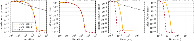
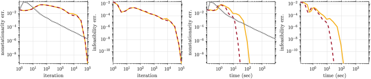
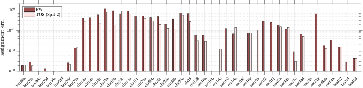
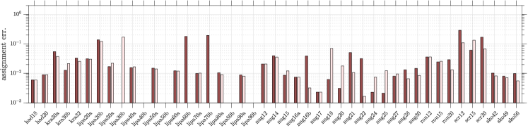
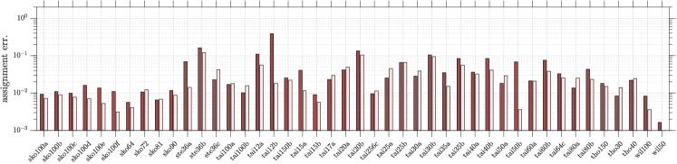
Figure 1: Empirical convergence of TOS for two different formulations ((Split 1) and (Split 2)) compared against FW for solving the relaxed QAP formulation (23). The [top] row corresponds to the results for the chr12a dataset and the [bottom] row for the esc128 dataset (from QAPLIB). In both cases, TOS exhibits locally linear convergence whereas FW converges sublinearly.

Figure 2: Assignment cost (see (26)) achieved by FW and TOS with the relax-and-round strategy for solving QAP. Smaller values are better, zero means a perfect estimation. Out of 134 QAP instances in the QAPLIB library, TOS outperforms FW on 83 problems; FW is better on 35; and the two methods get the same results on 16 instances.

6 Conclusions

We establish the convergence guarantees of TOS for minimizing the sum of three functions, one differentiable but potentially nonconvex and two convex but potentially nonsmooth. In contrast with the existing results, our analysis permits both nonsmooth terms to be indicator functions. Moreover, we extend our analysis for stochastic problems where we have access only to an unbiased estimator of the gradient of the differentiable term.

We present numerical experiments on QAPs. The empirical performance of the proposed method is promising. In our experience, the method converges to a stationary point with locally linear rates.

We conclude our paper with a short list of open questions and follow-up directions:
(i) We assume that $\mathrm{dom}(g)$ is bounded. This assumption is needed in our analysis since Definition 2 requires (4) to hold for all $x$ in $\mathrm{dom}(g)$. We can potentially drop this assumption by adopting a relaxed notion of stationarity where the inequality holds only on a feasible neighborhood of $\bar{z}$. Such measures are used in recent works for different problem models, e.g., see Definition 2.3 in (Nouiehed et al., 2019) and Definition 1 in (Song et al., 2020).
(ii) We did not explicitly use the smoothness of the differentiable term in our analysis. One can potentially derive tighter guarantees by using the smoothness or under additional assumptions such as the Kurdyka-Łojasiewicz property.
(iii) For the stochastic setting, we can improve the stochastic gradient complexity by using variance reduction techniques.
(iv) Developing an efficient implementation (that benefits from parallel computation) with an aim to investigate the full potential of TOS for solving QAP and other nonconvex problems such as the constrained and regularized neural networks is an important piece of future work.

Appendix A Algorithm

We focus on the Three Operator Splitting (TOS) method (Davis & Yin, 2017). We initialize the method from an arbitrary $y_{1}\in\mathrm{dom}(g)$. Then, the algorithm performs the following steps for $t=1,2,\ldots,T$:

$$z_{t} =\mathrm{prox}_{\gamma_{t}g}(y_{t})$$ (S.1)

$$x_{t} =\mathrm{prox}_{\gamma_{t}h}(2z_{t}-y_{t}-\gamma_{t}u_{t})$$ (S.2)

$$y_{t+1} =y_{t}-z_{t}+x_{t}$$ (S.3)

After $T$ iterations, the algorithm draws $\tau$ uniformly at random from $\{1,2,\ldots,T\}$ and returns $z_{\tau}$. We use $u_{t}=\nabla f(z_{t})$ in the deterministic setting and $u_{t}$ is an unbiased estimator of $\nabla f(z_{t})$ in the stochastic case.

A.1 TOS for Minimizing the Sum of More Than Three Functions

When the objective function consists of more than three terms, we can construct an equivalent formulation with three terms via a simple product space technique (Briceño-Arias, 2015), see Section 3.1 for the details. An application of TOS for solving this product space reformulation is detailed in Algorithm 2.

Algorithm 2 TOS for Problem (17) via product space formulation (18)

  Input: Initial points $y_{1}^{(i)}\in\mathbb{R}^{n}$ for $i=0,1,\ldots,m$, and a step-size sequence $\{\gamma_{t}\}_{t=1}^{T}$

  for $t=1,2,\ldots,T$ do

     for $i=0,1,2,\ldots,m$ do

        $z_{t}^{(i)}=\mathrm{prox}_{\gamma_{t}g_{i}}(y_{t}^{(i)})$

     end for

     $x_{t}=\frac{1}{m+1}\Big{(}\sum_{i=0}^{m}\big{(}2z_{t}^{(i)}-y_{t}^{(i)}\big{)}-\gamma_{t}\nabla f(z_{t}^{(0)})\Big{)}$

     for $i=0,1,2,\ldots,m$ do

        $y_{t+1}^{(i)}=y_{t}^{(i)}-z_{t}^{(i)}+x_{t}$

     end for

  end for

  Return: Draw $\tau$ uniformly at random from $\{1,2,\ldots,T\}$ and output ${z}_{\tau}$.

Appendix B Preliminaries

Lemma 1 (Prox-theorem).

Let $f:\mathbb{R}^{n}\to\mathbb{R}\cup\{+\infty\}$ be a proper closed and convex function. Then, for any $x,u\in\mathbb{R}^{n}$, the followings are equivalent:

1. $y=\mathrm{prox}_{f}(x)$.

2. $x-y\in\partial f(y)$.

3. $\langle x-y,z-y\rangle\leq f(z)-f(y)$  for any  $z\in\mathrm{dom}(f)$.
   

Lemma 2 (Cosine rule).

The following identity holds for any $x,y\in\mathbb{R}^{n}$:

$$\langle x,y\rangle=\frac{1}{2}\|x+y\|^{2}-\frac{1}{2}\|x\|^{2}-\frac{1}{2}\|y\|^{2}.$$

Lemma 3.

Suppose $f(x)=\mathbb{E}_{\xi}[\tilde{f}(x,\xi)]$ where $\xi$ is a random variable with distribution $\mathcal{P}$. Assume
(i) $\nabla\tilde{f}(x,\xi)$ is an unbiased estimator of $\nabla f(x)$, i.e., $\mathbb{E}_{\xi}[\nabla\tilde{f}(x,\xi)]=\nabla f(x),~{}\forall x\in\mathbb{R}^{n},$
(ii) $\nabla\tilde{f}(x,\xi)$ has bounded variance, i.e., there exists $\sigma<+\infty$ such that $\mathbb{E}_{\xi}[\|\nabla\tilde{f}(x,\xi)-\nabla f(x)\|^{2}]\leq\sigma^{2},~{}\forall x\in\mathbb{R}^{n}.$
Let $u=\frac{1}{|Q|}\sum_{\xi\in Q}\nabla\tilde{f}(x,\xi)$, where $Q$ is a set of $|Q|$ i.i.d. realizations from $\mathcal{P}$. Then, $u$ is an unbiased estimator of $\nabla f(x)$, and it satisfies the following variance bound:

$$\mathbb{E}_{Q}[\|u-\nabla f(x)\|^{2}]\leq\frac{\sigma^{2}}{|Q|}.$$

Lemma 1 and Lemma 2 are elementary, we skip the proofs. For the proof of Lemma 3, we refer to Lemma 2 in (Yurtsever et al., 2019) or (Reddi et al., 2016b).

Lemma 4 (Stationary point).

$\bar{z}\in\mathrm{dom}(\phi)$ is a first-order stationary point of (1) if and only if

$$\langle\nabla f(\bar{z}),\bar{z}-x\rangle+g(\bar{z})-g(x)+h(\bar{z})-h(x)\leq 0,\qquad\forall x\in\mathrm{dom}(\phi).$$ (S.4)

Proof.

Recall the definition of a stationary point: $\bar{z}$ is a stationary point of $f+g+h$ if for all feasible directions $s$ at $\bar{z}$ there exist $u\in\partial g(\bar{z})$ and $v\in\partial h(\bar{z})$ such that $\langle\nabla f(\bar{z})+u+v,s\rangle\geq 0$. Therefore,

$$\langle\nabla f(\bar{z})+u+v,\bar{z}-x\rangle\leq 0,\qquad\forall x\in\mathrm{dom}(\phi).$$ (S.5)

Since $g$ and $h$ are convex, $g(\bar{z})-g(x)\leq\langle u,\bar{z}-x\rangle$ and $h(\bar{z})-h(x)\leq\langle v,\bar{z}-x\rangle$. Hence, (S.5) implies (S.4).

Next, we show the opposite direction. First, we recall the definition of the directional derivative. Given a point $\bar{z}$ and a feasible direction $s$, the directional derivative is

$$g^{\prime}(\bar{z},s)=\lim_{\alpha\to 0^{+}}\frac{g(\bar{z}+\alpha s)-g(\bar{z})}{\alpha}.$$

Since $g$ and $h$ are convex, we have $g^{\prime}(\bar{z},s)=\sup_{u\in\partial{g}(\bar{z})}\langle u,s\rangle$ and $h^{\prime}(\bar{z},s)=\sup_{v\in\partial{h}(\bar{z})}\langle v,s\rangle$.

Now, suppose (S.4) holds. We choose $x=\bar{z}+\alpha s$ where $s$ is an arbitrary feasible direction and $\alpha>0$, and we get

$$\langle\nabla f(\bar{z}),\alpha s\rangle+g(\bar{z}+\alpha s)-g(\bar{z})+h(\bar{z}+\alpha s)-h(\bar{z})\geq 0.$$

We divide both sides by $\alpha$ and take $\alpha\to 0^{+}$,

$$\langle\nabla f(\bar{z}),s\rangle+\sup_{u\in\partial{g}(\bar{z})}\langle u,s\rangle+\sup_{v\in\partial{h}(\bar{z})}\langle v,s\rangle\geq 0.$$

Hence, for any feasible direction $s$, there exist $u\in\partial g(\bar{z})$ and $v\in\partial h(\bar{z})$ such that $\langle\nabla f(\bar{z})+u+v,s\rangle\geq 0$, which means $\bar{z}$ is a stationary point. ∎

Appendix C The Key Lemma of TOS

The following lemma presents the common part of the analyses for the different settings that we consider in our paper.

Lemma 5.

Consider the model problem (1). Assume that the domain of $g$ is bounded by the diameter $D_{g}$, i.e., $\|x-y\|\leq D_{g}$ for all $x,y\in\mathrm{dom}(g).$ For simplicity, we suppose $y_{1}\in\mathcal{G}$ (otherwise the bound explicitly depends on $y_{1}$). Then, $z_{\tau}$ returned by TOS after $T$ iterations with a fixed step-size $\gamma_{t}=\gamma$ satisfies, for all $x\in\mathrm{dom}(\phi)$,

$$\mathbb{E}_{\tau}[\langle u_{\tau},x_{\tau}-x\rangle+g(z_{\tau})-g(x)+h(x_{\tau})-h(x)]+\frac{1}{2\gamma}\mathbb{E}_{\tau}[\|x_{\tau}-z_{\tau}\|]^{2} \leq\frac{D_{g}^{2}}{2\gamma T}.$$ (S.6)

Proof.

From the algorithm step (S.2) and Lemma 1, we have

$$\langle 2z_{t}-y_{t}-\gamma_{t}u_{t}-x_{t},x-x_{t}\rangle\leq\gamma_{t}h(x)-\gamma_{t}h(x_{t}),\quad\forall x\in\mathrm{dom}(h).$$

We rearrange this inequality as follows:

$$\langle u_{t},x_{t}-x\rangle+h(x_{t})-h(x) \leq\frac{1}{\gamma_{t}}\langle 2z_{t}-y_{t}-x_{t},x_{t}-x\rangle$$

$$=\frac{1}{\gamma_{t}}\langle z_{t}-y_{t},z_{t}-x\rangle+\frac{1}{\gamma_{t}}\langle z_{t}-y_{t},x_{t}-z_{t}\rangle+\frac{1}{\gamma_{t}}\langle z_{t}-x_{t},x_{t}-x\rangle$$

$$=\frac{1}{\gamma_{t}}\langle z_{t}-y_{t},z_{t}-x\rangle+\frac{1}{\gamma_{t}}\langle y_{t}-z_{t}+x_{t}-x,z_{t}-x_{t}\rangle$$

$$=\frac{1}{\gamma_{t}}\langle z_{t}-y_{t},z_{t}-x\rangle+\frac{1}{\gamma_{t}}\langle y_{t+1}-x,y_{t}-y_{t+1}\rangle,\quad\forall x\in\mathrm{dom}(h).$$

Next, we bound the first term on the right hand side by using Lemma 1 again (but this time for the update step (S.1)):

$$\langle u_{t},x_{t}-x\rangle+g(z_{t})-g(x)+h(x_{t})-h(x)\leq\frac{1}{\gamma_{t}}\langle y_{t+1}-x,y_{t}-y_{t+1}\rangle,\quad\forall x\in\mathrm{dom}(\phi).$$

Due to Lemma 2 and the update step (S.3), we get, for all $x\in\mathrm{dom}(\phi)$

$$\langle u_{t},x_{t}-x\rangle+g(z_{t})-g(x)+h(x_{t})-h(x) \leq\frac{1}{2\gamma_{t}}\Big{(}\|y_{t}-x\|^{2}-\|y_{t+1}-x\|^{2}-\|y_{t+1}-y_{t}\|^{2}\Big{)}$$

$$=\frac{1}{2\gamma_{t}}\Big{(}\|y_{t}-x\|^{2}-\|y_{t+1}-x\|^{2}-\|x_{t}-z_{t}\|^{2}\Big{)}.$$

We use a fixed step-size $\gamma_{t}=\gamma>0$, sum this inequality over $t=1,2,\ldots,T$ and divide by $T$:

$$\frac{1}{T}\sum_{t=1}^{T}\left(\langle u_{t},x_{t}-x\rangle+g(z_{t})-g(x)+h(x_{t})-h(x)+\frac{1}{2\gamma}\|x_{t}-z_{t}\|^{2}\right) \leq\frac{1}{2\gamma T}\|y_{1}-x\|^{2}.$$ (S.7)

Note that, $\|y_{1}-x\|\leq D_{g}$ since both $x$ and $y_{1}$ are in $\mathrm{dom}(g)$. We choose $\tau$ uniformly at random from $1,2,\ldots,T$. By definition of the expectation, we get

$$\mathbb{E}_{\tau}[\langle u_{\tau},x_{\tau}-x\rangle+g(z_{\tau})-g(x)+h(x_{\tau})-h(x)]+\frac{1}{2\gamma}\mathbb{E}_{\tau}[\|x_{\tau}-z_{\tau}\|^{2}] \leq\frac{D_{g}^{2}}{2\gamma T},\quad\forall x\in\mathrm{dom}(\phi).$$

We complete the proof by using $\mathbb{E}[\|x_{\tau}-z_{\tau}\|]^{2}\leq\mathbb{E}[\|x_{\tau}-z_{\tau}\|^{2}]$. ∎

Appendix D Proof of Theorem 1 and Theorem 2

Theorem 1. Consider the model problem (1) under the following assumptions:
(i) The domain of $g$ is bounded with diameter $D_{g}$, i.e., $\|x-y\|\leq D_{g},~{}\forall x,y\in\mathrm{dom}(g)$.
(ii) $g$ is $L_{g}$-Lipschitz continuous on its domain, i.e., $g(x)-g(y)\leq L_{g}\|x-y\|,~{}\forall x,y\in\mathrm{dom}(g)$.
(iii) The gradient of $f$ is bounded by $G_{f}$ on the domain of $g$, i.e., $\|\nabla f(x)\|\leq G_{f},~{}\forall x\in\mathrm{dom}(g)$.
(iv) $h$ is $L_{h}$-Lipschitz continuous on $\mathbb{R}^{n}$, i.e., $h(x)-h(y)\leq L_{h}\|x-y\|,~{}\forall x,y\in\mathbb{R}^{n}.$
Choose $y_{1}\in\mathrm{dom}(g)$. Then, $z_{\tau}$ returned by TOS after $T$ iterations with the fixed step-size $\gamma=\frac{D_{g}}{2(G_{f}+L_{g}+L_{h})T^{2/3}}$ satisfies

$$\mathbb{E}_{\tau}[\langle\nabla f(z_{\tau}),z_{\tau}-x\rangle+g(z_{\tau})-g(x)+h(z_{\tau})-h(x)]\\ \leq D_{g}(G_{f}+L_{g}+L_{h})\frac{1}{T^{1/3}}+D_{g}(G_{f}+L_{h})\left(\frac{1}{T^{2/3}}+\frac{1}{T^{1/2}}+\frac{1}{T^{1/3}}\right),\quad\forall x\in\mathrm{dom}(\phi).$$

Proof.

From Lemma 5, we know

$$\mathbb{E}_{\tau}[\langle\nabla f(z_{\tau}),x_{\tau}-x\rangle+g(z_{\tau})-g(x)+h(x_{\tau})-h(x)]+\frac{1}{2\gamma}\mathbb{E}_{\tau}[\|x_{\tau}-z_{\tau}\|]^{2} \leq\frac{D_{g}^{2}}{2\gamma T},\quad\forall x\in\mathrm{dom}(\phi).$$

Based on assumptions (iii) and (iv),

$$\mathbb{E}_{\tau}[\langle\nabla f(z_{\tau}),z_{\tau}-x\rangle +g(z_{\tau})-g(x)+h(z_{\tau})-h(x)]+\frac{1}{2\gamma}\mathbb{E}_{\tau}[\|x_{\tau}-z_{\tau}\|]^{2}$$

$$\leq\frac{D_{g}^{2}}{2\gamma T}+\mathbb{E}_{\tau}[\langle\nabla f(z_{\tau}),z_{\tau}-x_{\tau}\rangle+h(z_{\tau})-h(x_{\tau})]$$

$$\leq\frac{D_{g}^{2}}{2\gamma T}+(G_{f}+L_{h})\,\mathbb{E}_{\tau}[\|z_{\tau}-x_{\tau}\|],\quad\forall x\in\mathrm{dom}(\phi).$$ (S.8)

At the same time, from assumptions (i), (ii), (iii) and (iv), we have

$$\mathbb{E}_{\tau}[\langle\nabla f(z_{\tau}),z_{\tau}-x\rangle+g(z_{\tau})-g(x)+h(z_{\tau})-h(x)] \geq-(G_{f}+L_{g}+L_{h})\mathbb{E}_{\tau}[\|z_{\tau}-x\|]$$

$$\geq-(G_{f}+L_{g}+L_{h})D_{g},\quad\forall x\in\mathrm{dom}(\phi).$$ (S.9)

Combining (S.8) and (S.9), we obtain the following second order inequality of $\mathbb{E}_{\tau}[\|x_{\tau}-z_{\tau}\|]$:

$$\frac{1}{2\gamma}\mathbb{E}_{\tau}[\|x_{\tau}-z_{\tau}\|]^{2}-(G_{f}+L_{h})\,\mathbb{E}_{\tau}[\|z_{\tau}-x_{\tau}\|]-\frac{D_{g}^{2}}{2\gamma T}-(G_{f}+L_{g}+L_{h})D_{g}\leq 0.$$

Solving this inequality leads to the following bound:

$$\mathbb{E}_{\tau}[\|z_{\tau}-x_{\tau}\|]\leq 2\gamma(G_{f}+L_{h})+\frac{D_{g}}{T^{1/2}}+\sqrt{2\gamma(G_{f}+L_{g}+L_{h})D_{g}}.$$

After substituting the step-size $\gamma=\frac{D_{g}}{2(G_{f}+L_{g}+L_{h})T^{2/3}}$, this becomes

$$\mathbb{E}_{\tau}[\|z_{\tau}-x_{\tau}\|]\leq D_{g}\left(\frac{1}{T^{2/3}}+\frac{1}{T^{1/2}}+\frac{1}{T^{1/3}}\right).$$

We complete the proof by substituting this inequality back into (S.8). ∎

Corollary 1. Consider the model problem (1) under the following assumptions:
(i) $g$ is the indicator function of convex closed bounded set $\mathcal{G}\subseteq\mathbb{R}^{n}$ with diameter $D_{\mathcal{G}}:=\sup_{x,y\in\mathcal{G}}\|x-y\|$.
(ii) The gradient of $f$ is bounded by $G_{f}$ in the domain of $g$, i.e., $\|\nabla f(x)\|\leq G_{f},~{}\forall x\in\mathrm{dom}(g)$.
(iii) $h$ is $L_{h}$-Lipschitz continuous on $\mathbb{R}^{n}$, i.e., $h(x)-h(y)\leq L_{h}\|x-y\|,~{}\forall x,y\in\mathbb{R}^{n}.$
Choose $y_{1}\in\mathcal{G}$. Then, $z_{\tau}\in\mathcal{G}$ returned by TOS after $T$ iterations with the fixed step-size $\gamma=\frac{D_{\mathcal{G}}}{2(G_{f}+L_{h})T^{2/3}}$ satisfies

$$\mathbb{E}_{\tau}[\langle\nabla f(z_{\tau}),z_{\tau}-x\rangle+h(z_{\tau})-h(x)]\leq D_{g}(G_{f}+L_{h})\left(\frac{1}{T^{2/3}}+\frac{1}{T^{1/2}}+\frac{2}{T^{1/3}}\right),\quad\forall x\in\mathcal{G}.$$

Proof.

Corollary 1 is a direct consequence of Theorem 1 with $\mathrm{dom}(g)=\mathrm{dom}(\phi)=\mathcal{G}$. The assumptions (i) and (ii) from Theorem 1 hold with $D_{g}=D_{\mathcal{G}}$ and $L_{g}=0$. We can set $g(z_{\tau})=g(x)=0$ because both $z_{\tau}$ and $x$ are in $\mathcal{G}$. ∎

Theorem 2. Consider the model problem (2) under the following assumptions:
(i) $\mathcal{G}\subseteq\mathbb{R}^{n}$ is a bounded closed convex set with diameter $D_{\mathcal{G}}:=\sup_{x,y\in\mathcal{G}}\|x-y\|$.
(ii) The gradient of $f$ is bounded by $G_{f}$ on $\mathcal{G}$, i.e., $\|\nabla f(x)\|\leq G_{f},~{}\forall x\in\mathcal{G}$.
(iii) $\mathcal{H}\subseteq\mathbb{R}^{n}$ is a closed convex set.
Choose $y_{1}\in\mathcal{G}$. Then, $z_{\tau}$ returned by TOS after $T$ iterations with the fixed step-size $\gamma_{t}=\frac{D_{\mathcal{G}}}{2G_{f}T^{2/3}}$ satisfies:

$$\mathbb{E}_{\tau}[\mathrm{dist}(z_{\tau},\mathcal{H})] \leq D_{\mathcal{G}}\left(\frac{1}{T^{2/3}}+\frac{1}{T^{1/2}}+\frac{1}{T^{1/3}}\right),$$

$$\mathbb{E}_{\tau}[\langle\nabla f(z_{\tau}),z_{\tau}-x\rangle] \leq G_{f}D_{\mathcal{G}}\left(\frac{1}{T^{2/3}}+\frac{1}{T^{1/2}}+\frac{2}{T^{1/3}}\right),\quad\forall x\in\mathcal{G}\cap\mathcal{H}.$$

Proof.

The proof is similar to the proof of Theorem 1. We present the details for completeness.

Since $x_{\tau}\in\mathcal{H}$, $z_{\tau}\in\mathcal{G}$, and $x\in\mathcal{G}\cap\mathcal{H}$, we can simplify Lemma 5 as

$$\mathbb{E}_{\tau}[\langle\nabla f(z_{\tau}),x_{\tau}-x\rangle]+\frac{1}{2\gamma}\mathbb{E}_{\tau}[\|x_{\tau}-z_{\tau}\|]^{2}\leq\frac{D_{\mathcal{G}}^{2}}{2\gamma T},\quad\forall x\in\mathcal{G}\cap\mathcal{H}.$$

Using the Cauchy-Schwartz inequality and assumption (ii), we get

$$\mathbb{E}_{\tau}[\langle\nabla f(z_{\tau}),z_{\tau}-x\rangle]+\frac{1}{2\gamma}\mathbb{E}[\|x_{\tau}-z_{\tau}\|]^{2} \leq\frac{D_{\mathcal{G}}^{2}}{2\gamma T}+\mathbb{E}_{\tau}[\langle\nabla f(z_{\tau}),z_{\tau}-x_{\tau}\rangle]$$

$$\leq\frac{D_{\mathcal{G}}^{2}}{2\gamma T}+\mathbb{E}_{\tau}[\|\nabla f(z_{\tau})\|\|z_{\tau}-x_{\tau}\|]$$

$$\leq\frac{D_{\mathcal{G}}^{2}}{2\gamma T}+G_{f}\mathbb{E}_{\tau}[\|z_{\tau}-x_{\tau}\|],\quad\forall x\in\mathcal{G}\cap\mathcal{H}.$$ (S.10)

At the same time, from the assumptions (i) and (ii), we have

$$\mathbb{E}_{\tau}[\langle\nabla f(z_{\tau}),z_{\tau}-x\rangle]\geq-\mathbb{E}_{\tau}[\|\nabla f(z_{\tau})\|\|z_{\tau}-x\|]\geq-G_{f}D_{\mathcal{G}},\quad\forall x\in\mathcal{G}\cap\mathcal{H}.$$ (S.11)

Combining (D) and (S.11), we obtain the following second order inequality of $\mathbb{E}_{\tau}[\|x_{\tau}-z_{\tau}\|]$:

$$\frac{1}{2\gamma}\mathbb{E}_{\tau}[\|x_{\tau}-z_{\tau}\|]^{2}-G_{f}\mathbb{E}_{\tau}[\|z_{\tau}-x_{\tau}\|]-\frac{D_{\mathcal{G}}^{2}}{2\gamma T}-G_{f}D_{\mathcal{G}}\leq 0.$$

Solving this inequality leads to the following bound:

$$\mathbb{E}_{\tau}[\|z_{\tau}-x_{\tau}\|]\leq 2G_{f}\gamma+\frac{D_{\mathcal{G}}}{T^{1/2}}+\sqrt{2\gamma G_{f}D_{\mathcal{G}}}.$$

After substituting the step-size $\gamma=\frac{D_{\mathcal{G}}}{2G_{f}T^{2/3}}$, this becomes

$$\mathbb{E}_{\tau}[\|z_{\tau}-x_{\tau}\|]\leq D_{\mathcal{G}}\left(\frac{1}{T^{2/3}}+\frac{1}{T^{1/2}}+\frac{1}{T^{1/3}}\right).$$ (S.12)

By definition, $\mathbb{E}_{\tau}[\mathrm{dist}(z_{\tau},\mathcal{H})]=\mathbb{E}_{\tau}[\inf_{x\in\mathcal{H}}\|z_{\tau}-x\|]\leq\mathbb{E}_{\tau}[\|z_{\tau}-x_{\tau}\|]$. Hence, we obtained the desired bound on the infeasibility error. Finally, the bound on the nonstationarity error follows by substituting (S.12) into (D). ∎

Appendix E Proof of Theorem 3 and Theorem 4

Theorem 3. Consider the model problem (19) under the following assumptions:
(i) The domain of $g$ is bounded with diameter $D_{g}$, i.e., $\|x-y\|\leq D_{g},~{}\forall x,y\in\mathrm{dom}(g).$
(ii) $g$ is $L_{g}$-Lipschitz continuous on its domain, i.e., $g(x)-g(y)\leq L_{g}\|x-y\|,~{}\forall x,y\in\mathrm{dom}(g).$
(iii) The gradient of $f$ is bounded by $G_{f}$ on the domain of $g$, i.e., $\|\nabla f(x)\|\leq G_{f},~{}\forall x\in\mathrm{dom}(g)$.
(iv) $h$ is $L_{h}$-Lipschitz continuous on $\mathbb{R}^{n}$, i.e., $h(x)-h(y)\leq L_{h}\|x-y\|,~{}\forall x,y\in\mathbb{R}^{n}$.
(v) $\nabla\tilde{f}(x,\xi)$ is an unbiased estimator of $\nabla f(x)$, i.e., $\mathbb{E}_{\xi}[\nabla\tilde{f}(x,\xi)]=\nabla f(x),~{}\forall x\in\mathbb{R}^{n}$.
(vi) $\nabla\tilde{f}(x,\xi)$ has bounded variance, i.e., there exists $\sigma<+\infty$ such that $\mathbb{E}_{\xi}[\|\nabla\tilde{f}(x,\xi)-\nabla f(x)\|^{2}]\leq\sigma^{2},~{}\forall x\in\mathbb{R}^{n}.$
Choose $y_{1}\in\mathrm{dom}(g)$. Use TOS with the stochastic gradient estimator

$$u_{t}:=\frac{1}{|Q_{t}|}\sum_{\xi\in Q_{t}}\nabla\tilde{f}(z_{t},\xi),$$

where $Q_{t}$ is a set of $|Q_{t}|$ i.i.d. realizations from distribution $\mathcal{P}$. Use the fixed mini-batch size $|Q_{t}|=|Q|=\Big{\lceil}\frac{T^{2/3}}{2(G_{f}+L_{g}+L_{h})^{2}}\Big{\rceil}$, and the fixed step-size $\gamma_{t}=\gamma=\frac{D_{g}}{2(G_{f}+L_{g}+L_{h})T^{2/3}}$ where $T$ is the total number of iterations. Then, $z_{\tau}$ returned by the algorithm satisfies:

$$\mathbb{E}_{\tau}\mathbb{E}[\langle\nabla f(z_{t}),z_{t}-x\rangle+g(z_{t})-g(x)+h(z_{t})-h(x)]\\ \leq D_{g}(G_{f}+L_{g}+L_{h})\frac{2+\sigma^{2}}{T^{1/3}}+D_{g}(G_{f}+L_{h})\left(\frac{2}{T^{2/3}}+\frac{\sqrt{4+2\sigma^{2}}}{T^{1/2}}+\frac{\sqrt{2}}{T^{1/3}}\right),\quad\forall x\in\mathrm{dom}(\phi).$$

Proof.

The proof follows similarly to the proof of Theorem 1 but we need to take care of the noise and variance terms. From Lemma 5, we have for all $x\in\mathrm{dom}(\phi)$,

$$\frac{1}{T}\sum_{t=1}^{T}\left(\langle u_{t},x_{t}-x\rangle+g(z_{t})-g(x)+h(x_{t})-h(x)+\frac{1}{2\gamma}\|x_{t}-z_{t}\|^{2}\right) \leq\frac{D_{g}^{2}}{2\gamma T}.$$ (S.13)

We first focus on the inner product term. Let us decompose it as

$$\langle u_{t},x_{t}-x\rangle=\langle\nabla f(z_{t}),z_{t}-x\rangle+\langle\nabla f(z_{t}),x_{t}-z_{t}\rangle+\langle u_{t}-\nabla f(z_{t}),z_{t}-x\rangle+\langle u_{t}-\nabla f(z_{t}),x_{t}-z_{t}\rangle.$$

Using the Cauchy-Schwartz inequality, Young’s inequality, and the assumptions (i) and (iii), we get

$$\langle u_{t},x_{t}-x\rangle \geq\langle\nabla f(z_{t}),z_{t}-x\rangle-G_{f}\|x_{t}-z_{t}\|-\frac{1}{\alpha}\|u_{t}-\nabla f(z_{t})\|^{2}-\frac{\alpha}{2}\|z_{t}-x\|^{2}-\frac{\alpha}{2}\|z_{t}-x_{t}\|^{2}$$

$$\geq\langle\nabla f(z_{t}),z_{t}-x\rangle-G_{f}\|x_{t}-z_{t}\|-\frac{1}{\alpha}\|u_{t}-\nabla f(z_{t})\|^{2}-\frac{\alpha}{2}D_{g}^{2}-\frac{\alpha}{2}\|z_{t}-x_{t}\|^{2},\quad\forall\alpha>0.$$

We take the expectation of both sides (over $Q_{t}$) and use Lemma 3 to get, for all $\alpha>0$,

$$\mathbb{E}[\langle u_{t},x_{t}-x\rangle] \geq\mathbb{E}[\langle\nabla f(z_{t}),z_{t}-x\rangle]-G_{f}\mathbb{E}[\|x_{t}-z_{t}\|]-\frac{\sigma^{2}}{\alpha|Q|}-\frac{\alpha}{2}D_{g}^{2}-\frac{\alpha}{2}\mathbb{E}[\|z_{t}-x_{t}\|^{2}].$$ (S.14)

Now, we take the expectation of (S.13) and substitute (S.14) into this inequality. This leads to

$$\frac{1}{T}\sum_{t=1}^{T}\mathbb{E}\Big{[}\langle\nabla f(z_{t}),z_{t}-x\rangle+g(z_{t})-g(x) +h(x_{t})-h(x)+\Big{(}\frac{1}{2\gamma}-\frac{\alpha}{2}\Big{)}\|x_{t}-z_{t}\|^{2}-G_{f}\|x_{t}-z_{t}\|\Big{]}$$

$$\leq\frac{D_{g}^{2}}{2\gamma T}+\frac{\alpha D_{g}^{2}}{2}+\frac{\sigma^{2}}{\alpha|Q|},\quad\forall x\in\mathrm{dom}(\phi),~{}\forall\alpha>0.$$ (S.15)

Based on the assumption (iv), we obtain

$$\frac{1}{T}\sum_{t=1}^{T}\mathbb{E}\Big{[}\langle\nabla f(z_{t}),z_{t}-x\rangle+g(z_{t})-g(x)+h(z_{t})-h(x)+\Big{(}\frac{1}{2\gamma}-\frac{\alpha}{2}\Big{)}\|x_{t}\!-\!z_{t}\|^{2}-(G_{f}+L_{h})\|x_{t}\!-\!z_{t}\|\Big{]}\\ \leq\frac{D_{g}^{2}}{2\gamma T}+\frac{\alpha D_{g}^{2}}{2}+\frac{\sigma^{2}}{\alpha|Q|},\quad\forall x\in\mathrm{dom}(\phi),~{}\forall\alpha>0.$$ (S.16)

At the same time, based on the assumptions (i), (ii), (iii), and (iv), we have

$$\langle\nabla f(z_{t}),z_{t}-x\rangle+g(z_{t})-g(x)+h(z_{t})-h(x)\geq-(G_{f}+L_{g}+L_{h})D_{g},\quad\forall x\in\mathrm{dom}(\phi).$$ (S.17)

Substituting (S.17) back into (S.16) leads to

$$\frac{1}{T}\sum_{t=1}^{T}\mathbb{E}\Big{[}\Big{(}\frac{1}{2\gamma}-\frac{\alpha}{2}\Big{)}\|x_{t}-z_{t}\|^{2}-(G_{f}+L_{h})\|x_{t}-z_{t}\|\Big{]}\leq\frac{D_{g}^{2}}{2\gamma T}+\frac{\alpha D_{g}^{2}}{2}+\frac{\sigma^{2}}{\alpha|Q|}+(G_{f}+L_{g}+L_{h})D_{g},$$

for all $\alpha>0$. We choose $\tau$ uniformly random over $1,2,\ldots,T$. Hence, by definition of the expectation over $\tau$, we have $\forall\alpha>0$,

$$\Big{(}\frac{1}{2\gamma}-\frac{\alpha}{2}\Big{)}\mathbb{E}_{\tau}\mathbb{E}[\|x_{\tau}\!-\!z_{\tau}\|^{2}]-(G_{f}\!+\!L_{h})\mathbb{E}_{\tau}\mathbb{E}[\|x_{\tau}\!-\!z_{\tau}\|]\leq\frac{D_{g}^{2}}{2\gamma T}+\frac{\alpha D_{g}^{2}}{2}+\frac{\sigma^{2}}{\alpha|Q|}+(G_{f}\!+\!L_{g}\!+\!L_{h})D_{g}.$$

Choose $\alpha$ such that $\alpha\leq\frac{1}{\gamma}$. Note that, $\mathbb{E}_{\tau}\mathbb{E}[\|x_{\tau}-z_{\tau}\|]^{2}\leq\mathbb{E}_{\tau}\mathbb{E}[\|x_{\tau}-z_{\tau}\|^{2}]$. Therefore,

$$\Big{(}\frac{1}{2\gamma}-\frac{\alpha}{2}\Big{)}\mathbb{E}_{\tau}\mathbb{E}[\|x_{\tau}\!-\!z_{\tau}\|]^{2}-(G_{f}\!+\!L_{h})\mathbb{E}_{\tau}\mathbb{E}[\|x_{\tau}\!-\!z_{\tau}\|]\leq\frac{D_{g}^{2}}{2\gamma T}+\frac{\alpha D_{g}^{2}}{2}+\frac{\sigma^{2}}{\alpha|Q|}+(G_{f}\!+\!L_{g}\!+\!L_{h})D_{g}.$$

We choose $\gamma=\frac{D_{g}}{2(G_{f}+L_{g}+L_{h})T^{2/3}}$, $\alpha=\frac{2(G_{f}+L_{g}+L_{h})}{D_{g}T^{1/3}}$, and $|Q|=\lceil\frac{T^{2/3}}{2(G_{f}+L_{g}+L_{h})^{2}}\rceil$. This leads to

$$\Big{(}\frac{T-1}{T}\Big{)}\mathbb{E}_{\tau}\mathbb{E}[\|x_{\tau}-z_{\tau}\|]^{2}-\frac{D_{g}}{T^{2/3}}\mathbb{E}_{\tau}\mathbb{E}[\|x_{\tau}-z_{\tau}\|]\leq D_{g}^{2}\left(\frac{2}{T}+\frac{\sigma^{2}}{T}+\frac{1}{T^{2/3}}\right).$$

By solving this inequality, we obtain, for any $T\geq 2$,

$$\mathbb{E}_{\tau}\mathbb{E}[\|x_{\tau}-z_{\tau}\|]\leq D_{g}\left(\frac{T^{1/3}}{T-1}+\sqrt{\frac{2+\sigma^{2}}{T-1}+\frac{T^{1/3}}{T-1}}\right)\leq D_{g}\left(\frac{2}{T^{2/3}}+\frac{\sqrt{4+2\sigma^{2}}}{T^{1/2}}+\frac{\sqrt{2}}{T^{1/3}}\right).$$ (S.18)

Combining this bound back again with (S.16), we get

$$\mathbb{E}_{\tau}\mathbb{E}[\langle\nabla f(z_{t}),z_{t}-x\rangle\!+\!g(z_{t})\!-\!g(x)\!+\!h(z_{t})\!-\!h(x)]\leq\frac{D_{g}^{2}}{2\gamma T}\!+\!\frac{\alpha D_{g}^{2}}{2}\!+\!\frac{\sigma^{2}}{\alpha|Q|}+(G_{f}+L_{h})\mathbb{E}_{\tau}\mathbb{E}[\|x_{t}-z_{t}\|]$$

$$\leq D_{g}(G_{f}+L_{g}+L_{h})\frac{2+\sigma^{2}}{T^{1/3}}+D_{g}(G_{f}+L_{h})\left(\frac{2}{T^{2/3}}+\frac{\sqrt{4+2\sigma^{2}}}{T^{1/2}}+\frac{\sqrt{2}}{T^{1/3}}\right),\quad\forall x\in\mathrm{dom}(\phi).$$

This completes the proof. ∎

Theorem 4. Consider the model problem (21) under the following assumptions:
(i) $\mathcal{G}\subseteq\mathbb{R}^{n}$ is a bounded closed convex set with diameter $D_{\mathcal{G}}:=\sup_{x,y\in\mathcal{G}}\|x-y\|$.
(ii) The gradient of $f$ is bounded by $G_{f}$ on $\mathcal{G}$, i.e., $\|\nabla f(x)\|\leq G_{f},~{}\forall x\in\mathcal{G}$.
(iii) $\mathcal{H}\subseteq\mathbb{R}^{n}$ is a closed convex set.
(iv) $\nabla\tilde{f}(x,\xi)$ is an unbiased estimator of $\nabla f(x)$, i.e., $\mathbb{E}_{\xi}[\nabla\tilde{f}(x,\xi)]=\nabla f(x),~{}\forall x\in\mathbb{R}^{n}$.
(v) $\nabla\tilde{f}(x,\xi)$ has bounded variance, i.e., there exists $\sigma<+\infty$ such that $\mathbb{E}_{\xi}[\|\nabla\tilde{f}(x,\xi)-\nabla f(x)\|^{2}]\leq\sigma^{2},~{}\forall x\in\mathbb{R}^{n}$.
Choose $y_{1}\in\mathcal{G}$. Use TOS with the stochastic gradient estimator

$$u_{t}:=\frac{1}{|Q_{t}|}\sum_{\xi\in Q_{t}}\nabla\tilde{f}(z_{t},\xi),$$

where $Q_{t}$ is a set of $|Q_{t}|$ i.i.d. realizations from distribution $\mathcal{P}$. Use the fixed mini-batch size $|Q_{t}|=|Q|=\lceil\frac{T^{2/3}}{2G_{f}^{2}}\rceil$, and the fixed step-size $\gamma_{t}=\gamma=\frac{D_{\mathcal{G}}}{2G_{f}T^{2/3}}$ where $T$ is the total number of iterations. Then, $z_{\tau}$ returned by the algorithm satisfies:

$$\mathbb{E}_{\tau}\mathbb{E}[\mathrm{dist}(z_{\tau},\mathcal{H})] \leq D_{\mathcal{G}}\left(\frac{2}{T^{2/3}}+\frac{\sqrt{4+2\sigma^{2}}}{T^{1/2}}+\frac{\sqrt{2}}{T^{1/3}}\right).$$

$$\mathbb{E}_{\tau}\mathbb{E}[\langle\nabla f(z_{\tau}),z_{\tau}-x\rangle] \leq G_{f}D_{\mathcal{G}}\left(\frac{2}{T^{2/3}}+\frac{\sqrt{4+2\sigma^{2}}}{T^{1/2}}+\frac{2+\sqrt{2}+\sigma^{2}}{T^{1/3}}\right),\quad\forall x\in\mathcal{G}\cap\mathcal{H}.$$

Proof.

The proof of Theorem 4 follows similarly to the proof of Theorem 3 until (E). Since $x_{\tau}\in\mathcal{H}$, $z_{\tau}\in\mathcal{G}$, and $x\in\mathcal{G}\cap\mathcal{H}$, we can simplify (E) as, $\forall x\in\mathcal{G}\cap\mathcal{H},~{}\forall\alpha>0$,

$$\frac{1}{T}\sum_{t=1}^{T}\mathbb{E}\Big{[}\langle\nabla f(z_{t}),z_{t}-x\rangle+\Big{(}\frac{1}{2\gamma}-\frac{\alpha}{2}\Big{)}\|x_{t}-z_{t}\|^{2}-G_{f}\|x_{t}-z_{t}\|\Big{]}\leq\frac{D_{\mathcal{G}}^{2}}{2\gamma T}+\frac{\alpha D_{\mathcal{G}}^{2}}{2}+\frac{\sigma^{2}}{\alpha|Q|}.$$ (S.19)

From the assumptions (i) and (ii), we have $\langle\nabla f(z_{t}),z_{t}-x\rangle\geq-G_{f}D_{\mathcal{G}}$. By definition of the expectation over $\tau$, we get,

$$\Big{(}\frac{1}{2\gamma}-\frac{\alpha}{2}\Big{)}\mathbb{E}_{\tau}\mathbb{E}[\|x_{\tau}-z_{\tau}\|^{2}]-G_{f}\mathbb{E}_{\tau}\mathbb{E}[\|x_{\tau}-z_{\tau}\|]\leq\frac{D_{\mathcal{G}}^{2}}{2\gamma T}+\frac{\alpha D_{\mathcal{G}}^{2}}{2}+\frac{\sigma^{2}}{\alpha|Q|}+G_{f}D_{\mathcal{G}},\quad\forall\alpha>0.$$

By substituting $|Q|=\lceil\frac{T^{2/3}}{2G_{f}^{2}}\rceil$ and $=\gamma=\frac{D_{\mathcal{G}}}{2G_{f}T^{2/3}}$, and choosing $\alpha=\frac{2G_{f}}{D_{\mathcal{G}}T^{1/3}}$, we get

$$\Big{(}\frac{T-1}{T}\Big{)}\mathbb{E}_{\tau}\mathbb{E}[\|x_{\tau}-z_{\tau}\|]^{2}-\frac{D_{\mathcal{G}}}{T^{2/3}}\mathbb{E}_{\tau}\mathbb{E}[\|x_{\tau}-z_{\tau}\|]\leq D_{\mathcal{G}}^{2}\left(\frac{2}{T}+\frac{\sigma^{2}}{T}+\frac{1}{T^{2/3}}\right).$$

Solving this inequality for $\mathbb{E}_{\tau}\mathbb{E}[\|x_{\tau}-z_{\tau}\|]$ yields

$$\mathbb{E}_{\tau}\mathbb{E}[\|x_{\tau}-z_{\tau}\|]\leq D_{\mathcal{G}}\left(\frac{T^{1/3}}{T-1}+\sqrt{\frac{2+\sigma^{2}}{T-1}+\frac{T^{1/3}}{T-1}}\right)\leq D_{\mathcal{G}}\left(\frac{2}{T^{2/3}}+\frac{\sqrt{4+2\sigma^{2}}}{T^{1/2}}+\frac{\sqrt{2}}{T^{1/3}}\right).$$ (S.20)

By definition, $\mathbb{E}_{\tau}\mathbb{E}[\mathrm{dist}(z_{\tau},\mathcal{H})]\leq\mathbb{E}_{\tau}\mathbb{E}[\|x_{\tau}-z_{\tau}\|]$.

To obtain the desired bound on the nonstationarity error, we substitute (S.20) into (S.19):

$$\mathbb{E}_{\tau}\mathbb{E}[\langle\nabla f(z_{\tau}),z_{\tau}-x\rangle] \leq\frac{D_{\mathcal{G}}^{2}}{2\gamma T}+\frac{\alpha D_{\mathcal{G}}^{2}}{2}+\frac{\sigma^{2}}{\alpha|Q|}+G_{f}\mathbb{E}_{\tau}\mathbb{E}[\|x_{t}-z_{t}\|],$$

$$\leq G_{f}D_{\mathcal{G}}\left(\frac{2}{T^{2/3}}+\frac{\sqrt{4+2\sigma^{2}}}{T^{1/2}}+\frac{2+\sqrt{2}+\sigma^{2}}{T^{1/3}}\right),\quad\forall x\in\mathcal{G}\cap\mathcal{H}.$$

This completes the proof. ∎

Appendix F Additional Details on the Numerical Experiments

This section presents more details about the QAP experiments in Section 5.

F.1 On the Projection onto $\mathcal{H}$ for (Split 2)

We consider the projection onto $\mathcal{H}:=\{X\in\mathbb{R}^{n\times n}:X1_{n}=1_{n},X^{\top}1_{n}=1_{n}\}$. Below, we present the derivation of the closed form formula for this projection from (Zass & Shashua, 2006; Lu et al., 2016).

We can formulate this problem as

$$\begin{aligned} &\min_{X\in\mathbb{R}^{n\times n}}&&\frac{1}{2}\|X_{\tau}-X\|_{F}^{2}\\ &\mathrm{subj.~{}to}&&X1_{n}=1_{n},\quad X^{\top}1_{n}=1_{n}.\end{aligned}$$ (S.21)

We use the Karush-Kuhn-Tucker (KKT) optimality conditions. We can write the Lagrangian of (S.21) as

$$\mathcal{L}(X,\mu_{1},\mu_{2})=\frac{1}{2}\|X_{\tau}-X\|_{F}^{2}+\langle\mu_{1},X1_{n}-1_{n}\rangle+\langle\mu_{2},X^{\top}1_{n}-1_{n}\rangle.$$

Then, the Lagrangian stationarity condition yields

$$\nabla_{X}\mathcal{L}(X,\mu_{1},\mu_{2})=X-X_{\tau}+\mu_{1}1_{n}^{\top}+1_{n}\mu_{2}^{\top}.$$ (S.22)

Our goal is to find a triplet $(X,\mu_{1},\mu_{2})\in\mathbb{R}^{n\times n}\times\mathbb{R}^{n}\times\mathbb{R}^{n}$ that satisfies

$$\nabla_{X}\mathcal{L}(X,\mu_{1},\mu_{2})=0,\quad X1_{n}=1_{n},\quad\text{and}\quad X^{\top}1_{n}=1_{n}.$$ (S.23)

Based on (S.22), the first condition (Lagrangian stationarity) leads to

$$X_{\tau}=X+\mu_{1}1_{n}^{\top}+1_{n}\mu_{2}^{\top}.$$ (S.24)

We multiply this by $1_{n}$ from the right, and by $1_{n}^{\top}$ from the left:

$$X_{\tau}1_{n}=X1_{n}+\mu_{1}1_{n}^{\top}1_{n}+1_{n}\mu_{2}^{\top}1_{n}=1_{n}+n\mu_{1}+1_{n}1_{n}^{\top}\mu_{2},$$ (S.25)

where we also used the feasibility condition in (S.23).

Let us try to find a solution with $\mu_{1}=\mu_{2}=\mu$. Under this assumption, (S.25) becomes

$$X_{\tau}1_{n}=1_{n}+(nI+1_{n}1_{n}^{\top})\mu\quad\iff\quad\mu=(nI+1_{n}1_{n}^{\top})^{-1}(X_{\tau}-I)1_{n}.$$ (S.26)

We can do the inversion by using the Sherman–Morrison formula:

$$(nI+1_{n}1_{n}^{\top})^{-1}=\frac{1}{n}I-\frac{1}{2n^{2}}1_{n}1_{n}^{\top}.$$ (S.27)

By substituting (S.27) back into (S.26), we get

$$\mu=\left(\frac{1}{n}I-\frac{1}{2n^{2}}1_{n}1_{n}^{\top}\right)(X_{\tau}-I)1_{n}=\frac{1}{n}X_{\tau}1_{n}-\frac{1}{2n^{2}}1_{n}1_{n}^{\top}X_{\tau}1_{n}-\frac{1}{2n}1_{n}.$$ (S.28)

Finally, we get $X$ by replacing (S.28) into (S.24) and rearranging the order:

$$X =X_{\tau}-\left(\frac{1}{n}X_{\tau}1_{n}-\frac{1}{2n^{2}}1_{n}1_{n}^{\top}X_{\tau}1_{n}-\frac{1}{2n}1_{n}\right)1_{n}^{\top}-1_{n}\left(\frac{1}{n}X_{\tau}1_{n}-\frac{1}{2n^{2}}1_{n}1_{n}^{\top}X_{\tau}1_{n}-\frac{1}{2n}1_{n}\right)^{\top}$$

$$=X_{\tau}-\frac{1}{n}X_{\tau}1_{n}1_{n}^{\top}+\frac{1_{n}^{\top}X_{\tau}1_{n}}{n^{2}}1_{n}1_{n}^{\top}-\frac{1}{n}1_{n}1_{n}^{\top}X_{\tau}^{\top}+\frac{1}{n}1_{n}1_{n}^{\top}.$$

$(X,\mu,\mu)$ satisfy the KKT conditions in (S.23), hence $X$ is a solution to (S.21).

F.2 On the Rounding Procedure for QAP: Projection onto the Set of Permutation Matrices

Suppose $X_{\tau}$ is a solution to (23). A natural rounding strategy is to find the nearest permutation matrix, i.e., projecting $X_{\tau}$ onto the set of permutation matrices. We can do this by solving a linear assignment problem (LAP). Below, we present a proof for this classical result.

The projection onto the set of permutation matrices can be formulated as

$$\begin{aligned} &\min_{X\in\mathbb{R}^{n\times n}}&&\frac{1}{2}\|X_{\tau}-X\|_{F}^{2}\\ &\mathrm{subj.~{}to}&&X\in\{0,1\}^{n\times n},~{}~{}X1_{n}=X^{\top}1_{n}=1_{n},\end{aligned}$$ (S.29)

where $I$ denotes the $n\times n$ identity matrix and $1_{n}$ is the $n$-dimensional vector of ones.

Recall that a permutation matrix has precisely one entry equal to $1$ in each row and column, and the other entries are $0$. Hence, $\|X\|_{F}=n$ for all permutation matrices. Then,

$$\|X_{\tau}-X\|_{F}^{2} =\|X_{\tau}\|_{F}^{2}-2\langle X_{\tau},X\rangle+\|X\|_{F}^{2}=\|X_{\tau}\|_{F}^{2}-2\langle X_{\tau},X\rangle+n^{2}.$$

Therefore, (S.29) is equivalent (in the sense that their solution sets are the same) to the following problem:

$$\begin{aligned} &\max_{X\in\mathbb{R}^{n\times n}}&&\langle X_{\tau},X\rangle\\ &\mathrm{subj.~{}to}&&X\in\{0,1\}^{n\times n},~{}~{}X1_{n}=X^{\top}1_{n}=1_{n}.\end{aligned}$$

Since the objective is linear, convex hull relaxation of the domain does not change the solution. Hence, the following problem is also equivalent:

$$\begin{aligned} &\max_{X\in\mathbb{R}^{n\times n}}&&\langle X_{\tau},X\rangle\\ &\mathrm{subj.~{}to}&&X\in[0,1]^{n\times n},~{}~{}X1_{n}=X^{\top}1_{n}=1_{n}.\end{aligned}$$

This is an instance of LAP. It can be solved in $\mathcal{O}(n^{3})$ time via the the Hungarian method (Kuhn, 1955; Munkres, 1957) or the Jonker-Volgenant algorithm (Jonker & Volgenant, 1987).

References

- Barbero & Sra (2018) Barbero, A. and Sra, S. Modular proximal optimization for multidimensional total-variation regularization. The Journal of Machine Learning Research, 19(1):2232–2313, 2018.
- Bian & Zhang (2020) Bian, F. and Zhang, X. A three-operator splitting algorithm for nonconvex sparsity regularization. arXiv preprint arXiv:2006.08951, 2020.
- Briceño-Arias (2015) Briceño-Arias, L. M. Forward–Douglas–Rachford splitting and forward-partial inverse method for solving monotone inclusions. Optimization, 64(5):1239–1261, 2015.
- Burkard et al. (1997) Burkard, R. E., Karisch, S. E., and Rendl, F. QAPLIB–a quadratic assignment problem library. Journal of Global optimization, 10(4):391–403, 1997.
- Cevher et al. (2018) Cevher, V., Vũ, B. C., and Yurtsever, A. Stochastic forward Douglas-Rachford splitting method for monotone inclusions. In Large-Scale and Distributed Optimization, pp. 149–179. Springer, 2018.
- Ciao (2011) Ciao, Y. Hungarian algorithm for linear assignment problems (v2.3). (Retrieved December 6, 2019), 2011. URL https://www.mathworks.com/matlabcentral/fileexchange/20652-hungarian-algorithm-for-linear-assignment-problems-v2-3.
- Condat (2016) Condat, L. Fast projection onto the simplex and the ball. Mathematical Programming, 158(1):575–585, 2016.
- Davis & Yin (2017) Davis, D. and Yin, W. A three-operator splitting scheme and its optimization applications. Set-valued and variational analysis, 25(4):829–858, 2017.
- De Berg et al. (2010) De Berg, M., Van Nijnatten, F., Sitters, R., Woeginger, G. J., and Wolff, A. The traveling salesman problem under squared Euclidean distances. arXiv preprint arXiv:1001.0236, 2010.
- Defazio et al. (2014) Defazio, A., Bach, F., and Lacoste-Julien, S. Saga: A fast incremental gradient method with support for non-strongly convex composite objectives. Advances in Neural Information Processing Systems, 27, 2014.
- El Halabi & Cevher (2015) El Halabi, M. and Cevher, V. A totally unimodular view of structured sparsity. In Artificial Intelligence and Statistics, pp. 223–231. PMLR, 2015.
- Fang et al. (2018) Fang, C., Li, C. J., Lin, Z., and Zhang, T. Spider: Near-optimal non-convex optimization via stochastic path integrated differential estimator. Advances in Neural Information Processing Systems, 31, 2018.
- Frank & Wolfe (1956) Frank, M. and Wolfe, P. An algorithm for quadratic programming. Naval Research Logistics Quarterly, 3(1-2):95–110, 1956.
- He & Yuan (2015) He, B. and Yuan, X. On non-ergodic convergence rate of Douglas–Rachford alternating direction method of multipliers. Numerische Mathematik, 130(3):567–577, 2015.
- Higham & Strabić (2016) Higham, N. J. and Strabić, N. Anderson acceleration of the alternating projections method for computing the nearest correlation matrix. Numerical Algorithms, 72(4):1021–1042, 2016.
- Hoffmann (1992) Hoffmann, A. The distance to the intersection of two convex sets expressed by the distances to each of them. Mathematische Nachrichten, 157(1):81–98, 1992.
- Jacob et al. (2009) Jacob, L., Obozinski, G., and Vert, J.-P. Group lasso with overlap and graph lasso. In Proceedings of the 26th International Coference on Machine Learning, pp. 433–440, 2009.
- Jaggi (2013) Jaggi, M. Revisiting frank-wolfe: Projection-free sparse convex optimization. In International Conference on Machine Learning, pp. 427–435. PMLR, 2013.
- Johnson & Zhang (2013) Johnson, R. and Zhang, T. Accelerating stochastic gradient descent using predictive variance reduction. Advances in Neural Information Processing Systems, 26, 2013.
- Jonker & Volgenant (1987) Jonker, R. and Volgenant, A. A shortest augmenting path algorithm for dense and sparse linear assignment problems. Computing, 38(4):325–340, 1987.
- Koopmans & Beckmann (1957) Koopmans, T. C. and Beckmann, M. Assignment problems and the location of economic activities. Econometrica: journal of the Econometric Society, pp. 53–76, 1957.
- Kuhn (1955) Kuhn, H. W. The Hungarian method for the assignment problem. Naval research logistics quarterly, 2(1-2):83–97, 1955.
- Kundu et al. (2018) Kundu, A., Bach, F., and Bhattacharya, C. Convex optimization over intersection of simple sets: Improved convergence rate guarantees via an exact penalty approach. In International Conference on Artificial Intelligence and Statistics, pp. 958–967. PMLR, 2018.
- Lacoste-Julien (2016) Lacoste-Julien, S. Convergence rate of Frank-Wolfe for non-convex objectives. arXiv preprint arXiv:1607.00345, 2016.
- Liu & Yin (2019) Liu, Y. and Yin, W. An envelope for Davis–Yin splitting and strict saddle-point avoidance. Journal of Optimization Theory and Applications, 181(2):567–587, 2019.
- Loiola et al. (2007) Loiola, E. M., de Abreu, N. M. M., Boaventura-Netto, P. O., Hahn, P., and Querido, T. A survey for the quadratic assignment problem. European journal of operational research, 176(2):657–690, 2007.
- Lu et al. (2016) Lu, Y., Huang, K., and Liu, C.-L. A fast projected fixed-point algorithm for large graph matching. Pattern Recognition, 60:971–982, 2016.
- Malitsky (2019) Malitsky, Y. Golden ratio algorithms for variational inequalities. Mathematical Programming, pp. 1–28, 2019.
- Maronna et al. (2019) Maronna, R. A., Martin, R. D., Yohai, V. J., and Salibián-Barrera, M. Robust statistics: Theory and methods. John Wiley & Sons, 2019.
- McLachlan & Krishnan (1996) McLachlan, G. J. and Krishnan, T. The EM Algorithm and Extentions. Wiley, 1996.
- Munkres (1957) Munkres, J. Algorithms for the assignment and transportation problems. Journal of the society for industrial and applied mathematics, 5(1):32–38, 1957.
- Nguyen et al. (2017) Nguyen, L. M., Liu, J., Scheinberg, K., and Takáč, M. Sarah: A novel method for machine learning problems using stochastic recursive gradient. In International Conference on Machine Learning, pp. 2613–2621. PMLR, 2017.
- Nouiehed et al. (2019) Nouiehed, M., Sanjabi, M., Huang, T., Lee, J. D., and Razaviyayn, M. Solving a class of non-convex min-max games using iterative first order methods. Advances in Neural Information Processing Systems, 32, 2019.
- Ollila & Tyler (2014) Ollila, E. and Tyler, D. E. Regularized -estimators of scatter matrix. IEEE Transactions on Signal Processing, 62(22):6059–6070, 2014.
- Patrinos et al. (2014) Patrinos, P., Stella, L., and Bemporad, A. Douglas-Rachford splitting: Complexity estimates and accelerated variants. In 53rd IEEE Conference on Decision and Control, pp. 4234–4239. IEEE, 2014.
- Pedregosa & Gidel (2018) Pedregosa, F. and Gidel, G. Adaptive three operator splitting. In International Conference on Machine Learning, pp. 4085–4094, 2018.
- Pedregosa et al. (2019) Pedregosa, F., Fatras, K., and Casotto, M. Proximal splitting meets variance reduction. In The 22nd International Conference on Artificial Intelligence and Statistics, pp. 1–10. PMLR, 2019.
- Peyré et al. (2019) Peyré, G., Cuturi, M., et al. Computational optimal transport: With applications to data science. Foundations and Trends® in Machine Learning, 11(5-6):355–607, 2019.
- Raguet et al. (2013) Raguet, H., Fadili, J., and Peyré, G. A generalized forward-backward splitting. SIAM Journal on Imaging Sciences, 6(3):1199–1226, 2013.
- Reddi et al. (2016a) Reddi, S. J., Hefny, A., Sra, S., Poczos, B., and Smola, A. Stochastic variance reduction for nonconvex optimization. In International conference on machine learning, pp. 314–323. PMLR, 2016a.
- Reddi et al. (2016b) Reddi, S. J., Sra, S., Póczos, B., and Smola, A. Stochastic Frank-Wolfe methods for nonconvex optimization. In 2016 54th Annual Allerton Conference on Communication, Control, and Computing (Allerton), pp. 1244–1251. IEEE, 2016b.
- Richard et al. (2012) Richard, E., Savalle, P.-A., and Vayatis, N. Estimation of simultaneously sparse and low rank matrices. In Proceedings of the 29th International Coference on Machine Learning, pp. 51–58, 2012.
- Roux et al. (2012) Roux, N., Schmidt, M., and Bach, F. A stochastic gradient method with an exponential convergence rate for finite training sets. Advances in Neural Information Processing Systems, 25, 2012.
- Sahni & Gonzalez (1976) Sahni, S. and Gonzalez, T. P-complete approximation problems. Journal of the ACM (JACM), 23(3):555–565, 1976.
- Shivanna et al. (2015) Shivanna, R., Chatterjee, B., Sankaran, R., Bhattacharyya, C., and Bach, F. Spectral norm regularization of orthonormal representations for graph transduction. In Neural Information Processing Systems, 2015.
- Song et al. (2020) Song, C., Zhou, Z., Zhou, Y., Jiang, Y., and Ma, Y. Optimistic dual extrapolation for coherent non-monotone variational inequalities. Advances in Neural Information Processing Systems, 33, 2020.
- Themelis et al. (2018) Themelis, A., Stella, L., and Patrinos, P. Forward-backward envelope for the sum of two nonconvex functions: Further properties and nonmonotone linesearch algorithms. SIAM Journal on Optimization, 28(3):2274–2303, 2018.
- Vogelstein et al. (2015) Vogelstein, J. T., Conroy, J. M., Lyzinski, V., Podrazik, L. J., Kratzer, S. G., Harley, E. T., Fishkind, D. E., Vogelstein, R. J., and Priebe, C. E. Fast approximate quadratic programming for graph matching. PLOS one, 10(4):e0121002, 2015.
- Yurtsever et al. (2016) Yurtsever, A., Vũ, B. C., and Cevher, V. Stochastic three-composite convex minimization. In Proceedings of the 30th International Conference on Neural Information Processing Systems, pp. 4329–4337, 2016.
- Yurtsever et al. (2018) Yurtsever, A., Fercoq, O., Locatello, F., and Cevher, V. A conditional gradient framework for composite convex minimization with applications to semidefinite programming. In International Conference on Machine Learning, pp. 5727–5736. PMLR, 2018.
- Yurtsever et al. (2019) Yurtsever, A., Sra, S., and Cevher, V. Conditional gradient methods via stochastic path-integrated differential estimator. In International Conference on Machine Learning, pp. 7282–7291. PMLR, 2019.
- Zaslavskiy et al. (2008) Zaslavskiy, M., Bach, F., and Vert, J.-P. A path following algorithm for the graph matching problem. IEEE Transactions on Pattern Analysis and Machine Intelligence, 31(12):2227–2242, 2008.
- Zass & Shashua (2006) Zass, R. and Shashua, A. Doubly stochastic normalization for spectral clustering. Advances in neural information processing systems, 19, 2006.
- Zass & Shashua (2007) Zass, R. and Shashua, A. Nonnegative sparse PCA. In Advances in neural information processing systems, pp. 1561–1568, 2007.
- Zhao & Cevher (2018) Zhao, R. and Cevher, V. Stochastic three-composite convex minimization with a linear operator. In International Conference on Artificial Intelligence and Statistics, pp. 765–774. PMLR, 2018.
- Zong et al. (2018) Zong, C., Tang, Y., and Cho, Y. J. Convergence analysis of an inexact three-operator splitting algorithm. Symmetry, 10(11):563, 2018.