Anytime Ellipsoidal Over-approximation of Forward Reach Sets of Uncertain Linear Systems

Abstract.

Computing tight over-approximation of reach sets of a controlled uncertain dynamical system is a common practice in verification of safety-critical cyber-physical systems (CPS). While several algorithms are available for this purpose, they tend to be computationally demanding in CPS applications since here, the computational resources such as processor availability tend to be scarce, time-varying and difficult to model. A natural idea then is to design “computation-aware” algorithms that can dynamically adapt with respect to the processor availability in a provably safe manner. Even though this idea should be applicable in broader context, here we focus on ellipsoidal over-approximations. We demonstrate that the algorithms for ellipsoidal over-approximation of reach sets of uncertain linear systems, are well-suited for anytime implementation in the sense the quality of the over-approximation can be dynamically traded off depending on the computational time available, all the while guaranteeing safety. We give a numerical example to illustrate the idea, and point out possible future directions.

1. Introduction

A standard method to verify the performance in safety-critical cyber-physical systems (CPS) is to compute the over-approximation of forward reach sets, i.e., the set of states that the system can reach to at a given time, subject to uncertainties in its initial conditions, control input and unmeasured disturbance. Several numerical toolboxes have been developed for this purpose from different perspectives. For instance, the level set toolbox (Mitchell, 2008) utilizes the fact that the forward reach set is the zero sublevel set of the viscosity solution of certain Hamilton-Jacobi-Bellman partial differential equation associated with the controlled dynamics. There are parametric toolboxes which over-approximate the reach sets using simple geometric shapes such as the ellipsoids (Kurzhanskiy and Varaiya, 2006) and zonotopes (Althoff, 2015). There also exist recent works (Fan et al., 2017; Devonport and Arcak, 2020a, b) for data-driven over-approximation of the reach sets.

Over-approximating reach sets, even for linear systems, is computationally intensive especially in the presence of time-varying set-valued uncertainties. On the other hand, safety-critical CPS applications have scarce computational resource due to limitations in weight, power, and due to several software concurrently sharing the same hardware. A natural idea then is to design “computation-aware” over-approximation algorithms which can dynamically trade-off performance without compromising safety. In particular, one would like to design anytime algorithms (Zilberstein, 1995, 1996) which provably over-approximate the forward reach sets at any given time but the quality of over-approximation dynamically depends on the computational time available. As more computational time becomes available, the over-approximation becomes “tighter”.

While anytime algorithms have appeared before in systems-control literature (Bhattacharya and Balas, 2004; Fontanelli et al., 2008; Gupta, 2010; Quevedo et al., 2014; Pant et al., 2015; Liebenwein et al., 2018), their application in parametric over-approximation of the reach set as proposed herein, is new. Specifically, we consider forward reach sets of uncertain linear time-varying systems and point out that the ellipsoidal over-approximation algorithms are particularly suitable for anytime implementation. We summarize the motivations behind ellipsoidal over-approximation in Section 2. The overall computational framework is described in Sec. 3 including the models of dynamics and uncertainties, as well as the anytime ellipsoidal over-approximation algorithm. Sec. 4 details a numerical case study to illustrate the ideas. Concluding remarks and future directions are given in Sec. 5.

Notations

We use $\mathbb{N}$ to denote the set $\{1,2,\ldots\}$, and let $\mathbb{N}_{0}:=\mathbb{N}\cup\{0\}$. The set of $d\times d$ symmetric positive semidefinite (resp. definite) matrices is denoted as $\mathbb{S}_{+}^{d}$ (resp. $\mathbb{S}_{++}^{d}$). The matrix inequalities $\succeq\bm{0}$ (resp. $\succ\bm{0}$) denote positive semidefiniteness (resp. definiteness). A nondegenerate ellipsoid in $d$ dimensions with center vector $\bm{q}\in\mathbb{R}^{d}$ and shape matrix $\bm{Q}\in\mathbb{S}_{++}^{d}$ is given by

$$\mathcal{E}\left(\bm{q},\bm{Q}\right):=\{\bm{y}\in\mathbb{R}^{d}\mid\left(\bm{y}-\bm{q}\right)^{\top}\bm{Q}^{-1}\left(\bm{y}-\bm{q}\right)\leq 1\}.$$

We refer to it as the $\left(\bm{q},\bm{Q}\right)$ ellipsoidal parameterization. As in (Halder, 2018, Sec. I.2), we will also use the $\left(\bm{A}_{0},\bm{b}_{0},c_{0}\right)$ ellipsoidal parameterization encoding the quadratic form:

$$\mathcal{E}\left(\bm{A}_{0},\bm{b}_{0},c_{0}\right):=\{\bm{y}\in\mathbb{R}^{d}\mid\bm{y}^{\top}\bm{A}_{0}\bm{y}+2\bm{y}^{\top}\bm{b}_{0}+c_{0}\leq 1\}.$$

The $\left(\bm{A}_{0},\bm{b}_{0},c_{0}\right)$ and $\left(\bm{q},\bm{Q}\right)$ parameterizations are related by

(1a) $$\bm{A}_{0}=\bm{Q}^{-1},\quad\bm{b}_{0}=-\bm{Q}^{-1}\bm{q},\quad c_{0}=\bm{q}^{\top}\bm{Q}^{-1}\bm{q}-1,$$

(1b) $$\bm{Q}=\bm{A}_{0}^{-1},\quad\bm{q}=-\bm{Q}\bm{b}_{0}.$$

We use $\|\cdot\|_{2}$ to denote the Euclidean 2-norm, ${\rm{vol}}(\cdot)$ to denote the Lebesgue volume, $\lfloor\cdot\rfloor$ to denote the floor operator, and $\mathcal{O}(\cdot)$ for the standard Big-O notation. We use $\bm{0}_{m\times n}$ and $\bm{I}_{n}$ to denote the $m\times n$ zero matrix, and $n\times n$ identity matrx, respectively. We use $\bm{0}_{n}$ for $\bm{0}_{n\times n}$. The symbol $\bm{1}$ denotes a vector of ones of appropriate size. We use shorthands ${\rm{diag}}(\cdot)$ and ${\rm{blkdiag}}(\cdot)$ to denote the diagonal and the block diagonal matrices, respectively.

2. Why Ellipsoids

The are several reasons why ellipsoids are attractive as a parametric over-approximation primitive.

1. A nondegenerate ellipsoid in $d$ dimensions can be parameterized by $d(d+3)/2$ reals describing its center vector and the shape matrix. Unlike polytopes, this implies fixed parameterization complexity which is useful in CPS context, for example in designing communication protocols where the ellipsoidal descriptions need to be encoded in communication packets. Fixed bit-length parameterization is helpful to reduce the complexity of the communication protocol.

2. Time-varying ellipsoids naturally model norm bounded uncertainties ubiquitous in systems-control engineering. For example, in vehicular CPS applications, it is natural to represent uncertainties in exogenous disturbance (e.g., wind gust), estimation error and actuation noise as time-varying weighted norm bounds.

In the systems-control literature, ellipsoidal over-approximations have been well-investigated in the context of estimation (Schweppe, 1968; Witsenhausen, 1968; Bertsekas and Rhodes, 1971; Chernous’ko, 1980) and system identification (Fogel, 1979; Norton, 1987; Belforte et al., 1990; Kosut et al., 1992).

3. Framework

We next detail the models for dynamics and ellipsoidal set-valued uncertainties, and outline the nature of the computation for ellipsoidal over-approximation of the forward reach set.

3.1. Models

We consider a linear system

(2) $$\dot{\bm{x}}=\bm{A}(t)\bm{x}+\bm{B}(t)\bm{u}+\bm{G}(t)\bm{w},$$

with state $\bm{x}\in\mathbb{R}^{n}$, control input $\bm{u}\in\mathbb{R}^{m}$, and unmeasured disturbance $\bm{w}\in\mathbb{R}^{p}$. The system matrices $\bm{A}(t),\bm{B}(t),\bm{G}(t)$ are assumed to be continuous in time $t$, and are of commensurate dimensions.

Given the set-valued uncertainties in the initial condition $\bm{x}(0)\in\mathcal{X}_{0}$, control $\bm{u}\in\mathcal{U}(t)$, and disturbance $\bm{w}\in\mathcal{W}(t)$, we would like to approximate the forward reach set at time $t$ as

$$\mathcal{R}\left(\mathcal{X}_{0},t\right):=\{\bm{x}(t)\in\mathbb{R}^{n}\mid\> \dot{\bm{x}}=\bm{A}(t)\bm{x}+\bm{B}(t)\bm{u}+\bm{G}(t)\bm{w},$$

(3) $$\bm{x}(0)\in\mathcal{X}_{0},\bm{u}\in\mathcal{U}(t),\bm{w}\in\mathcal{W}(t)\}.$$

We suppose that the set-valued uncertainties are ellipsoidal: $\mathcal{X}_{0}=\mathcal{E}\left(\bm{x}_{0},\bm{X}_{0}\right)$, $\mathcal{U}(t)=\mathcal{E}\left(\bm{u}_{c}(t),\bm{U}(t)\right)$, and $\mathcal{W}(t)=\mathcal{E}\left(\bm{w}_{c}(t),\bm{W}(t)\right)$. In this case, the set $\mathcal{R}\left(\mathcal{X}_{0},t\right)$ is guaranteed to be convex compact.

For $k\in\mathbb{N}_{0}$, we consider the prediction horizon $\left[k\Delta t,\allowbreak(k+1)\Delta t\right]$ over which we would like to approximate (3). The reachable tube over this prediction horizon is

(4) $$\overline{\mathcal{R}}\left(\mathcal{X}_{0},t\right):=\bigcup_{t\in\left[k\Delta t,\allowbreak(k+1)\Delta t\right]}\mathcal{R}\left(\mathcal{X}_{0},t\right).$$

3.2. Ellipsoidal Over-approximation of $\mathcal{R}\left(\mathcal{X}_{0},t\right)$

We follow the ellipsoidal over-approximation procedure as in (Kurzhanskiy and Varaiya, 2006), (Kurzhanski and Varaiya, 2014, Ch. 3). The basic idea is to construct a family of ellipsoids $\{\mathcal{E}\allowbreak\left(\bm{x}_{c}(t),\allowbreak\bm{X}_{i}(t)\right)\}_{i=1}^{N}$ parameterized by unit vectors $\bm{\ell}_{i0}\in\mathbb{R}^{n}$ where $i=1,\ldots,N$. This parameterized family of ellipsoids are constructed such that for any finite $N\in\mathbb{N}$, we have

(5) $$\mathcal{R}\left(\mathcal{X}_{0},t\right)\subseteq\widehat{\mathcal{R}}_{N}\left(\mathcal{X}_{0},t\right):=\bigcap_{i=1}^{N}\mathcal{E}\allowbreak\left(\bm{x}_{c}(t),\allowbreak\bm{X}_{i}(t)\right),$$

and $\bigcap_{i=1}^{\infty}\mathcal{E}\allowbreak\left(\bm{x}_{c}(t),\allowbreak\bm{X}_{i}(t)\right)=\mathcal{R}\left(\mathcal{X}_{0},t\right)$. Notice that $\widehat{\mathcal{R}}_{N}$ being an intersection of ellipsoids, is guaranteed to be convex, but not an ellipsoid in general.

The center vector $\bm{x}_{c}(t)$ solves the initial value problem (IVP)

(6) $$\dot{\bm{x}}_{c}=\bm{A}(t)\bm{x}_{c}+\bm{B}(t)\bm{u}_{c}+\bm{G}(t)\bm{w}_{c},\quad\bm{x}_{c}(0)=\bm{x}_{0}.$$

Let $\bm{\ell}(t):=\exp\left(-\left(\bm{A}(t)\right)^{\top}t\right)\bm{\ell}_{i0}$, and

(7) $$\pi_{i}(t):=\left(\dfrac{\bm{\ell}_{i}^{\top}(t)\bm{B}(t)\bm{U}(t)\bm{B}^{\top}(t)\bm{\ell}_{i}(t)}{\bm{\ell}_{i}^{\top}(t)\bm{X}_{i}(t)\bm{\ell}_{i}(t)}\right)^{1/2}.$$

Furthermore, define the unit vectors

(8) $$\widehat{\bm{v}}_{1i}(t):=\dfrac{\bm{X}_{i}^{1/2}(t)\bm{\ell}_{i}(t)}{\|\bm{X}_{i}^{1/2}(t)\bm{\ell}_{i}(t)\|_{2}},\quad\widehat{\bm{v}}_{2i}(t):=\dfrac{\bm{G}(t)\bm{W}(t)\bm{G}^{\top}(t)\bm{\ell}_{i}(t)}{\|\bm{G}(t)\bm{W}(t)\bm{G}^{\top}(t)\bm{\ell}_{i}(t)\|_{2}},$$

and let $\bm{S}_{i}(t)$ be an $n\times n$ orthogonal matrix that solves

(9) $$\bm{S}_{i}(t)\widehat{\bm{v}}_{2i}(t)=\widehat{\bm{v}}_{1i}(t).$$

Ref. (Kurzhanski and Varaiya, 2014, Thm. 4.4.4) gives an algorithm to compute $\bm{S}_{i}(t)$ in (9) using $\mathcal{O}(n^{2})$ operations.

With the definitions (7), (8), (9) in place, the shape matrices $\bm{X}_{i}(t)$ solve the IVPs

$$\dot{\bm{X}}_{i}(t)=\bm{A}(t)\bm{X}_{i}(t)+\bm{X}_{i}(t)\left(\bm{A}(t)\right)^{\top}\!+\pi_{i}(t)\bm{X}_{i}(t)+\frac{1}{\pi_{i}(t)}\bm{B}(t)\bm{U}(t)\bm{B}^{\top}\!(t)$$

$$-\bm{X}_{i}^{1/2}(t)\bm{S}_{i}(t)\bm{G}(t)\bm{W}(t)\bm{G}^{\top}(t)-\bm{G}(t)\bm{W}(t)\bm{G}^{\top}(t)\bm{S}_{i}^{\top}(t)\bm{X}_{i}^{1/2}(t),$$

(10) $$\bm{X}_{i}(0)=\bm{X}_{0}.$$

Solving the IVPs (6) and (10) allow us to define $\widehat{\mathcal{R}}_{N}$ in (5) that is guaranteed to contain the true reach set $\mathcal{R}$ for any finite $N$. Increasing $N$ results in intersecting more ellipsoids, thus making the outer-approximation tighter. For the derivations of (6) and (10), we refer the readers to (Kurzhanski and Varaiya, 2014, Ch. 3) and (Kurzhanskiĭ and Vályi, 1997, Part III).

Now the question arises how to practically compute/approximate the intersection of a finite number of ellipsoids, which is what $\widehat{\mathcal{R}}_{N}$ is. For parsimony, a natural idea is to compute the minimum volume outer ellipsoid $\mathcal{E}\left(\bm{x}_{c}(t),\bm{X}(t)\right)$, a.k.a. the Löwner-John ellipsoid (John, 1948; Henk, 2012),(Grötschel et al., 1993, p. 69) containing $\widehat{\mathcal{R}}_{N}$, i.e., to solve

(11a) $$\underset{\bm{X}(t)}{\arg\min}\qquad{\rm{vol}}\left(\mathcal{E}\left(\bm{x}_{c}(t),\bm{X}(t)\right)\right)$$

(11b) $$\text{subject to}\quad\bigcap_{i=1}^{N}\mathcal{E}\allowbreak\left(\bm{x}_{c}(t),\allowbreak\bm{X}_{i}(t)\right)\subseteq\mathcal{E}\left(\bm{x}_{c}(t),\bm{X}(t)\right).$$

It is known (John, 1948), (Ben-Tal and Nemirovski, 2001, Thm. 3.7.1), (Grötschel et al., 1993, Thm. 3.1.9) that the Löwner-John ellipsoid exists and is unique for any compact convex set, and thus $\bm{X}(t)$ in (11) is unique too. However, (11) is a semi-infinite programming problem (Boyd and Vandenberghe, 2004, Ch. 8.4.1) that has no known exact semidefinite programming (SDP) reformulation. In fact, verifying (11b) for $N+1$ given ellipsoids $\{\mathcal{E}\allowbreak\left(\bm{x}_{c}(t),\allowbreak\bm{X}_{i}(t)\right)\}_{i=1}^{N},\mathcal{E}\left(\bm{x}_{c}(t),\bm{X}(t)\right)$, is NP-complete.

Several suboptimal reformulations of problem (11) are available (Boyd et al., 1994, Ch. 3.7.2); one of them is based on the S procedure (Yakubovich, 1971, 1992; Pólik and Terlaky, 2007) that works well in practice, see e.g., (Haddad and Halder, 2021, Sec. V). We will use this S procedure-based reformulation given by

(12a) $$\underset{\widetilde{\bm{A}},\widetilde{\bm{b}},\tau_{1},\ldots,\tau_{N}}{\text{minimize}}\quad\log\det\widetilde{\bm{A}}^{-1}$$

(12b) $$\text{subject to}\qquad\;\;\widetilde{\bm{A}}\succ\bm{0},$$

(12c) $$\qquad\qquad\qquad\;\;\tau_{1},\ldots,\tau_{N}\geq 0,$$

(12d) $$\begin{bmatrix}\widetilde{\bm{A}}&\widetilde{\bm{b}}&\bm{0}\\ \widetilde{\bm{b}}^{\top}&-1&\widetilde{\bm{b}}^{\top}\\ \bm{0}&\widetilde{\bm{b}}&-\widetilde{\bm{A}}\end{bmatrix}-\displaystyle\sum_{i=1}^{N}\tau_{i}\begin{bmatrix}\bm{A}_{i}&\bm{b}_{i}&\bm{0}\\ \bm{b}_{i}^{\top}&c_{i}&\bm{0}\\ \bm{0}&\bm{0}&\bm{0}\end{bmatrix}\preceq\bm{0}.$$

We note that (12) is a determinant maximization (max-det) problem subject to linear matrix inequality constraints (Vandenberghe et al., 1998) for which efficient algorithms are known. Let us denote the optimizer of (12) as

$$\left(\widetilde{\bm{A}}_{\text{opt}},\widetilde{\bm{b}}_{\text{opt}},\tau_{1_{\text{opt}}},\ldots,\tau_{N_{\text{opt}}}\right).$$

Problem (12) takes the ellipsoids

(13) $$\!\!\bigg{\{}\mathcal{E}\left(\left(\bm{X}_{i}(t)\right)^{-1}\!,-\left(\bm{X}_{i}(t)\right)^{-1}\!\bm{x}_{c}(t),\bm{x}_{c}^{\top}(t)\left(\bm{X}_{i}(t)\right)^{-1}\!\bm{x}_{c}(t)-1\right)\!\!\bigg{\}}_{i=1}^{N}\!$$

in $\left(\bm{A}_{0},\bm{b}_{0},c_{0}\right)$ parameterization as input at times $t=k\Delta t$, $k\in\mathbb{N}$. From (1b), its output in $\left(\bm{q},\bm{Q}\right)$ parameterization is the ellipsoid $\mathcal{E}\left(-\widetilde{\bm{A}}_{\text{opt}}^{-1}\widetilde{\bm{b}}_{\text{opt}},\widetilde{\bm{A}}_{\text{opt}}^{-1}\right)$, which is time-varying since the input data (13) is time-varying. If the input ellipsoids are $n$ dimensional, then the max-det problem (12) has $N+n(n+3)/2$ unknowns.

By construction, the Löwner-John ellipsoid $\mathcal{E}\left(\bm{x}_{c}(t),\bm{X}(t)\right)$, i.e., the optimal ellipsoid from (11), is contained in the optimal ellipsoid obtained from (12), i.e., in $\mathcal{E}\left(-\widetilde{\bm{A}}_{\text{opt}}^{-1}\widetilde{\bm{b}}_{\text{opt}},\widetilde{\bm{A}}_{\text{opt}}^{-1}\right)$.

3.3. Parallelization and Projection

3.3.1. Parallelizing ellipsoidal propagation

The ellipsoidal overapproximation procedure outlined in Sec. 3.2 involves propagating the center vector $\bm{x}_{c}(t)$ and the shape matrices $\bm{X}_{i}(t)$, followed by solving (12). Since the solution of the $N+1$ IVPs (6) and (10) are independent of each other, they may be run in parallel, if such computing resource is available. Furthermore, the fact that increasing (resp. descreasing) $N$ increases (resp. decreases) the accuracy while guaranteeing the inclusion (5), suggests an anytime implementation discussed in Sec. 3.4.

Suppose that the worst-case computational time for propagating $N$ ellipsoids is $t_{\text{propagation}}$. If the worst-case time for solving the IVP (6) is $t_{\text{center}}$, and the same for solving a single instance of the IVP (10) is $t_{\text{shape}}$, then $t_{\text{propagation}}=\max\{t_{\text{center}},\allowbreak t_{\text{shape}}\}$ provided parallel computing resource is available. If no parallel computing is available, then $t_{\text{propagation}}=t_{\text{center}}+Nt_{\text{shape}}$. We suppose that $t_{\text{center}}$ and $t_{\text{propagation}}$ are known beforehand (based on the IVP solver used).

3.3.2. Projection

It is often desired to over-approximate the reach sets of a subset of states. For example, in vehicular CPS applications such as unmanned aerial systems (UAS) and automated driving, ensuring real-time collision avoidance and safe separation amounts to checking distances between reach sets (or over-approximations thereof) in respective position coordinates; e.g., $(x,y,z)$ position coordinates for UAS applications, and $(x,y)$ position coordinates in automated driving applications.

Notice that since the dynamics remain coupled, the ellipsoidal propagation in Sec. 3.2 need to be done in the original state space $\mathbb{R}^{n}$. However, some computational savings is possible if one is only interested in approximating the reach sets of a subset of states. In such cases, instead of solving the max-det problem (12) over $n$ dimensional ellipsoids, one may project the propagated ellipsoids on the subset of states of interest, and then solve (12) over those smaller dimensional ellipsoids, resulting in a lower dimensional convex problem. To justify projection before solving (12), denote ${\rm{proj}}(\cdot)$ as the suitable projection map. Also, let $\mathcal{E}_{\rm{LJ}}(\cdot)$ as the Löwner-John operator, i.e., a set-valued operator that takes a compact set and returns its unique minimum volume outer ellipsoid. We appeal to the following relations:

(14a) $$\!\!\!\!{\rm{proj}}\left(\mathcal{E}_{\rm{LJ}}\left(\bigcap_{i=1}^{N}\mathcal{E}\left(\bm{x}_{c}(t),\bm{X}_{i}(t)\right)\right)\right)=\mathcal{E}_{\rm{LJ}}\left({\rm{proj}}\left(\bigcap_{i=1}^{N}\mathcal{E}\left(\bm{x}_{c}(t),\bm{X}_{i}(t)\right)\right)\right)$$

(14b) $$\!\!\!\!\subseteq\mathcal{E}_{\rm{LJ}}\left(\bigcap_{i=1}^{N}{\rm{proj}}\left(\mathcal{E}\left(\bm{x}_{c}(t),\bm{X}_{i}(t)\right)\right)\right)\subseteq\;\stackrel{{\scriptstyle\text{\normalsize{minimizer of (\ref{Sprocedure}) with}}}}{{\text{input }{\rm{proj}}(\cdot)\text{ of (\ref{InputDataForSprocedure}).}}}$$

The equality in (14a) holds because the operator $\mathcal{E}_{\rm{LJ}}(\cdot)$ commutes with any linear map (Boyd and Vandenberghe, 2004, Ch. 8.4.3). In (14b), the first set inclusion follows from the general fact that any transformation of intersection is included in the intersection of that transformation. The last set inclusion in (14b) holds by construction, i.e., because the minimizing ellipsoid of (12) is a superset of that of the (11) for an arbitrary set of input ellipsoids.

We note that projecting the $n$-dimensional ellipsoid to the appropriate axis-aligned subspace amounts to simply extracting the corresponding center subvectors and shape submatrices from the full-dimensional center vectors and shape matrices. The propagation and projection can be parallelized (across unit vectors $\{\bm{\ell}_{i0}\}_{i=1}^{N}$) if such computing resource is available.

3.4. Anytime Computation

For $k\in\mathbb{N}_{0}$, suppose that at the instance $t=k\Delta t$, we have $t_{\text{available}}<\Delta t$ time available to compute an over-approximation of the reach set $\mathcal{R}\left(\mathcal{X}_{0},t=(k+1)\Delta t\right)$. The prediction horizon length $\Delta t$ need not be small. The time $t_{\text{available}}$ will be governed by the processor availability, and may only be known at the instance $t=k\Delta t$. In general, $t_{\text{available}}$ depends on other software running concurrently on the CPS platform, and can have significant variability. Stochastic processor availability models (e.g., i.i.d., Markovian) have appeared before in the anytime control literature (Gupta, 2010; Quevedo et al., 2014).

Recall from Sec. 3.3.1 that $t_{\text{propagation}}$ is the worst-case computational time for ellipsoidal propagation. In case any projection on subset of states is performed, we ignore the associated small computational time in extracting the subvectors and submatrices. Suppose $t_{\text{opt}}$ is the worst-case computational time for solving (12), which has polynomial dependence on $N$ (Vandenberghe et al., 1998).

Our standing assumption is that $\Delta t$ is large enough to allow the computation in Sec. 3.2 with at least $N=1$ (even with no parallel computation), i.e., $t_{\text{center}}+t_{\text{shape}}\leq\Delta t$. Since the total computational time

(15) $$t_{\text{total}}=t_{\text{propagation}}+t_{\text{opt}}=f(N),$$

for some nonlinear $f$, a simple way to design the supervisory algorithm shown in Fig. 1 is to obtain a data-driven estimate $\widehat{f}$ for the function $f$ in (15), and then to determine $\widehat{N}$ as the maximal real root of

(16) $$t_{\text{available}}=\widehat{f}(\widehat{N}).$$

As per our assumption, $t_{\text{available}}$ is such that at least $N=1$ is feasible and thus (16) has at least one real root. Then $N_{\max}:=\lfloor\widehat{N}\rfloor$. In the numerical results presented in Sec. 4, we computed $\widehat{f}$ using polynomial regression.

The computation for $N_{\max}=1$ involves single ellipsoidal propagation, and no optimization.

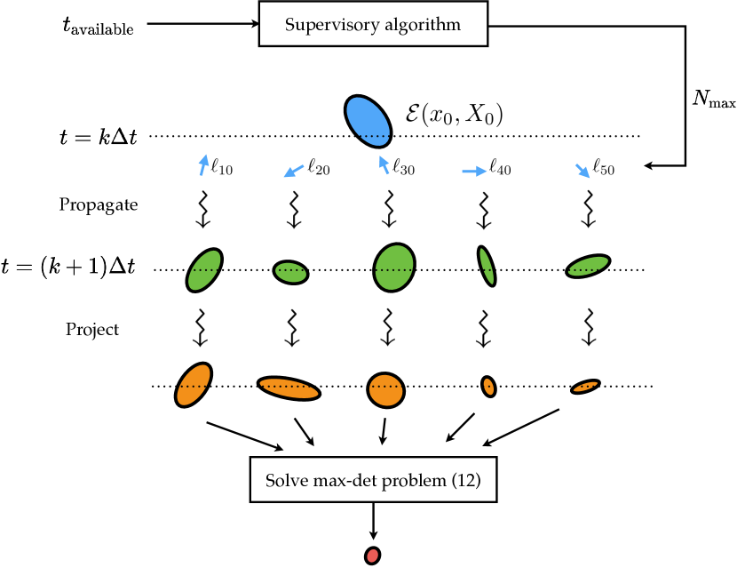
Figure 1. A schematic of the proposed anytime computational framework for the ellipsoidal over-approximation of forward reach set at time $t=(k+1)\Delta t$ based on the data at $t=k\Delta t$, $k\in\mathbb{N}_{0}$. Depending on $t_{\text{available}}<\Delta t$, the supervisory algorithm adapts the maximal number of unit vectors $N_{\max}$ (shown here $N_{\max}=5$) to minimize conservatism in over-approximation while preserving safety. The projection step may only be needed when one is interested to compute the reach set over a subset of states. The squiggly arrows denote possible parallelized computation.

4. Numerical Simulations

To illustrate the ideas presented in Sec. 3, we consider the linearized model of a standard quadrotor dynamics (see Fig. 2) with $n=12$ states, $m=4$ inputs, and $p=3$ unmeasured disturbances. The parameters in the model are shown in Table 1.

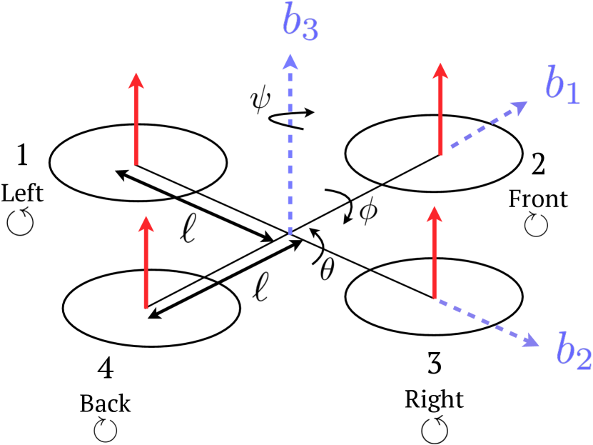
Figure 2. A schematic of the rotor numbering convention for the quadrotor dynamics in body frame $b_{1}b_{2}b_{3}$. The parameter $\ell$ denotes the arm length. Also shown are the Euler angles $(\phi,\theta,\psi)$.

The $12\times 1$ state vector $\bm{x}=\left(x,y,z,\phi,\theta,\psi,p,q,r,u,v,w\right)^{\top}$ comprises of the translational positions $(x,y,z)$ [m], the Euler angles $(\phi,\theta,\psi)$ [rad], the translational velocities $(u,v,w)$ [m/s], and the rotational velocities $(p,q,r)$ [rad/s]. For $i=1,\ldots,4$, the rotor angular velocities (in (rad/s)²) are $\omega_{i}^{2}=\overline{\omega}_{i}^{2}+u_{i}$, where the nominal rotor angular velocities $\left(\overline{\omega}_{1}^{2},\overline{\omega}_{2}^{2},\overline{\omega}_{3}^{2},\overline{\omega}_{4}^{2}\right)$ solve (from equating thrust to weight and angular torques to zero)

$$\left(\begin{array}[]{l}\overline{\omega}_{1}^{2}\\ \overline{\omega}_{2}^{2}\\ \overline{\omega}_{3}^{2}\\ \overline{\omega}_{4}^{2}\end{array}\right)=\left[\begin{array}[]{cccc}c_{\mathrm{T}}&c_{\mathrm{T}}&c_{\mathrm{T}}&c_{\mathrm{T}}\\ \ell c_{\mathrm{T}}&0&-\ell c_{\mathrm{T}}&0\\ 0&\ell c_{\mathrm{T}}&0&-\ell c_{\mathrm{T}}\\ c_{\mathrm{D}}&-c_{\mathrm{D}}&c_{\mathrm{D}}&-c_{\mathrm{D}}\end{array}\right]^{-1}\left(\begin{array}[]{c}mg\\ 0\\ 0\\ 0\end{array}\right).$$

The $4\times 1$ control vector is $\bm{u}=\left(u_{1},u_{2},u_{3},u_{4}\right)^{\top}$.

Symbols	Descriptions	Values [units]
$m$	mass of quadrotor	0.468 [kg]
$\ell$	arm length	0.225 [m]
${\rm{diag}}\left(J_{xx},J_{yy},J_{zz}\right)$	inertia matrix	${\rm{diag}}\left(5,5,9\right)\times 10^{-3}$ [N$\cdot$m$\cdot$s2]
$c_{\rm{T}}$	rotor thrust coefficient	$7.2\times 10^{-5}$ [N$\cdot$s2]
$c_{\rm{D}}$	drag coefficient	$1.1\times 10^{-5}$ [N$\cdot$m$\cdot$s2]
$g$	acceleration due to gravity	9.81 [m/s2]

Table 1. The parameters in the quadrotor model used in Sec. 4.

The linearized open-loop model is given by

(17) $$\dot{\bm{x}}=\bm{A}\bm{x}+\bm{B}\bm{u}+\bm{G}\bm{w},\quad\bm{G}:=\begin{bmatrix}\bm{0}_{6\times 3}\\ \bm{I}_{3}\\ \bm{0}_{3}\end{bmatrix},$$

i.e., the disturbance $\bm{w}(t)$ models wind gusts acting along the translational acceleration channels, and

$$\bm{A}:=\left[\begin{array}[]{llll}\bm{0}_{3}&\bm{0}_{3}&\bm{I}_{3}&\bm{0}_{3}\\ \bm{0}_{3}&\bm{0}_{3}&\bm{0}_{3}&\bm{I}_{3}\\ \bm{0}_{3}&\bm{\Gamma}&\bm{0}_{3}&\bm{0}_{3}\\ \bm{0}_{3}&\bm{0}_{3}&\bm{0}_{3}&\bm{0}_{3}\end{array}\right],\>\bm{\Gamma}:=\left[\begin{array}[]{ccc}0&-g&0\\ g&0&0\\ 0&0&0\end{array}\right],$$

$$\bm{B}:=\left[\begin{array}[]{c}\mathbf{0}_{3\times 4}\\ \mathbf{0}_{3\times 4}\\ \mathbf{0}_{2\times 4}\\ \frac{c_{\mathrm{T}}}{m}\mathbf{1}_{1\times 4}\\ \bm{\Lambda}_{3\times 4}\end{array}\right],\>\bm{\Lambda}_{3\times 4}:=\left[\begin{array}[]{cccc}\frac{\ell c_{\mathrm{T}}}{J_{xx}}&0&-\frac{\ell c_{\mathrm{T}}}{J_{xx}}&0\\ &&&\\ 0&\frac{\ell c_{\mathrm{T}}}{J_{yy}}&0&-\frac{\ell c_{\mathrm{T}}}{J_{yy}}\\ &&&\\ \frac{c_{\mathrm{D}}}{J_{zz}}&-\frac{c_{\mathrm{D}}}{J_{zz}}&\frac{c_{\mathrm{D}}}{J_{zz}}&-\frac{c_{\mathrm{D}}}{J_{zz}}\end{array}\right].$$

We close the loop around (17) using a finite horizon LQR controller

(18) $$\bm{u}(\cdot,t)=\bm{K}(t)\left(\cdot\right)+\bm{u}_{\text{feedforward}}(t)$$

synthesized to track desired path $(x_{d}(t),y_{d}(t),z_{d}(t))\equiv(\cos t,\sin t,t)$. In the quadratic cost function, we used the state cost weight matrix $\bm{Q}={\rm{blkdiag}}\left(1000\bm{I}_{3},{\rm{diag}}\left(1,1,10\right),\bm{I}_{6}\right)$, the control cost weight matrix $\bm{R}=0.1\bm{I}_{4}$, and the terminal cost weight matrix $\bm{M}={\rm{blkdiag}}\left(1000\bm{I}_{3},\bm{I}_{9}\right)$. As is well known (see e.g., (Anderson and Moore, 2007, Ch. 4)), the feedback gain $\bm{K}(t)=-\bm{R}^{-1}\bm{B}^{\top}\bm{P}(t)$ where $\bm{P}(t)$ solves the associated Riccati matrix ODE with terminal condition depending on $\bm{M}$, and that $\bm{u}_{\text{feedforward}}(t)=\bm{R}^{-1}\bm{B}^{\top}\bm{v}(t)$ where $\bm{v}(t)$ solves a vector ODE with terminal condition also depending on the matrix $\bm{M}$.

We suppose that the controller (18) acts on imperfect state estimate $\widehat{\bm{x}}(t)$ with underestimation error $\bm{\xi}(t):=\bm{x}(t)-\widehat{\bm{x}}(t)$. Letting

$$\bm{A}_{\rm{cl}}:=\bm{A}+\bm{B}\bm{K}(t),\quad\bm{B}_{\rm{cl}}:=\bm{B}\bm{R}^{-1}\bm{B}^{\top},\quad\bm{\eta}(t):=\bm{P}(t)\bm{\xi}(t)+\bm{v}(t),$$

the closed-loop dynamics can then be written as the linear time-varying system

(19) $$\dot{\bm{x}}=\bm{A}_{\rm{cl}}(t)\bm{x}+\bm{B}_{\rm{cl}}\bm{\eta}+\bm{G}\bm{w}.$$

We suppose that the estimation error $\bm{\xi}(t)\in\mathcal{E}\left(\bm{0}_{12\times 1},\bm{E}(t)\right)$ for known matrices $\bm{E}(t)$ which are $\succ\bm{0}$ at all $t$ and continuous in $t$. Consequently, $\bm{\eta}(t)\in\mathcal{E}\left(\bm{v}(t),\bm{V}(t)\right)$ with $\bm{V}(t):=\bm{P}(t)\bm{E}(t)\bm{P}^{\top}(t)$. Furthermore, $\bm{x}(0)\in\mathcal{E}\left(\bm{x}_{0},\bm{X}_{0}\right)$, $\bm{w}(t)\in\mathcal{E}\left(\bm{w}_{c}(t),\bm{W}(t)\right)$.

We followed the framework in Sec. 3 to propagate the ellipsoidal uncertainties in $12$ dimensional state space and then projected the same in the first three coordinates to obtain the ellipsoidal reach set over-approximation in $(x,y,z)$. We used $\bm{x}_{0}=(1,\bm{0}_{1\times 11})^{\top}$, $\bm{X}_{0}={\rm{diag}}\left(0.8147,0.4854,0.7431,0.0344,0.6551,0.9593,0.6160,\right.$ $\left.0.0540,0.1656,0.9961,0.4314,0.5132\right)^{\top}$, $\bm{E}(t)\equiv\bm{I}_{12}$, $\bm{w}_{c}(t)=\left(\cos t,\sin t,\cos t\right)^{\top}$, and $\bm{W}(t)\equiv 0.01\bm{I}_{3}$. All our simulations were done in MATLAB with (12) solved via cvx.

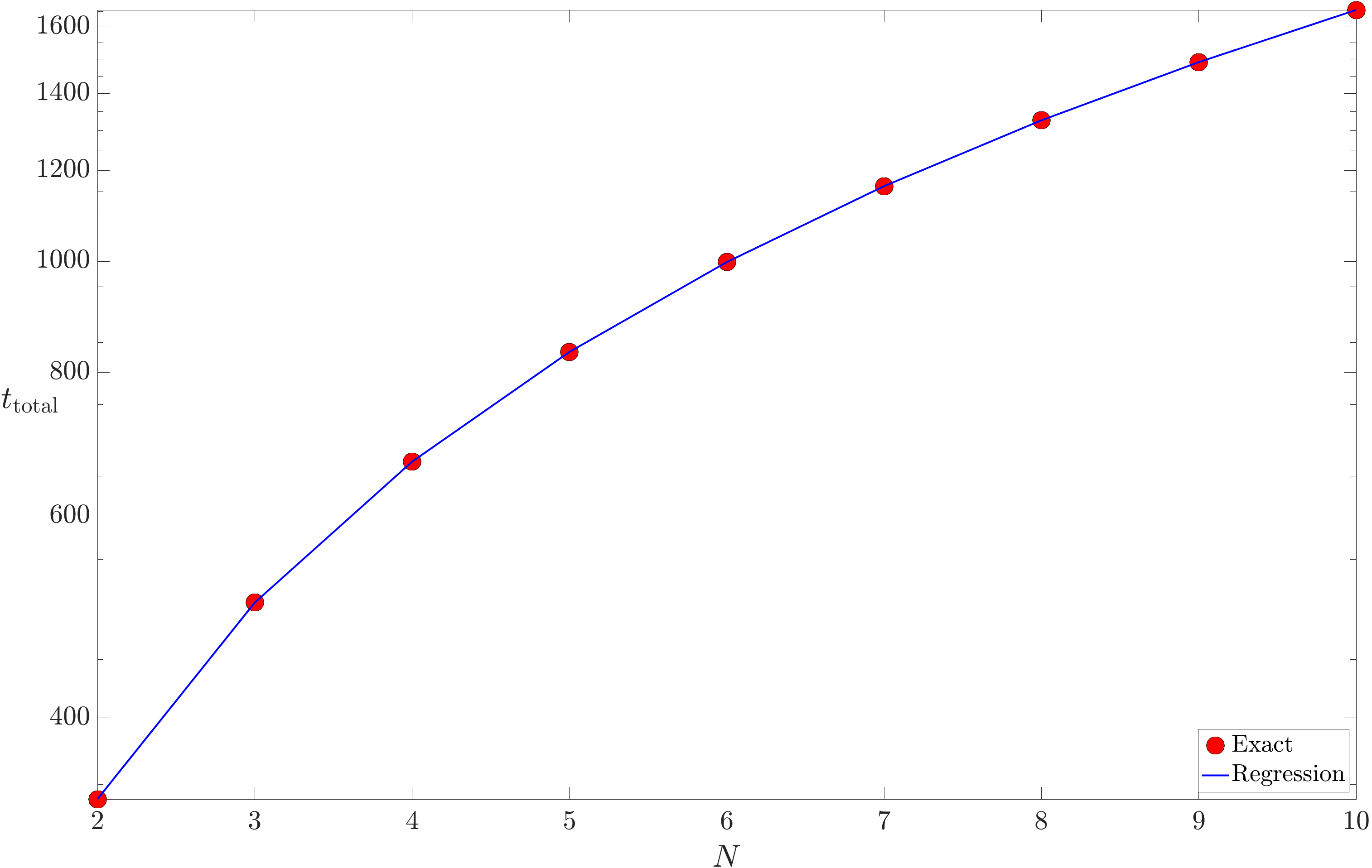
Figure 3. Data-driven fourth degree polynomial regression (least square) estimate $\widehat{f}$ for (15). The vertical axis is in [s].

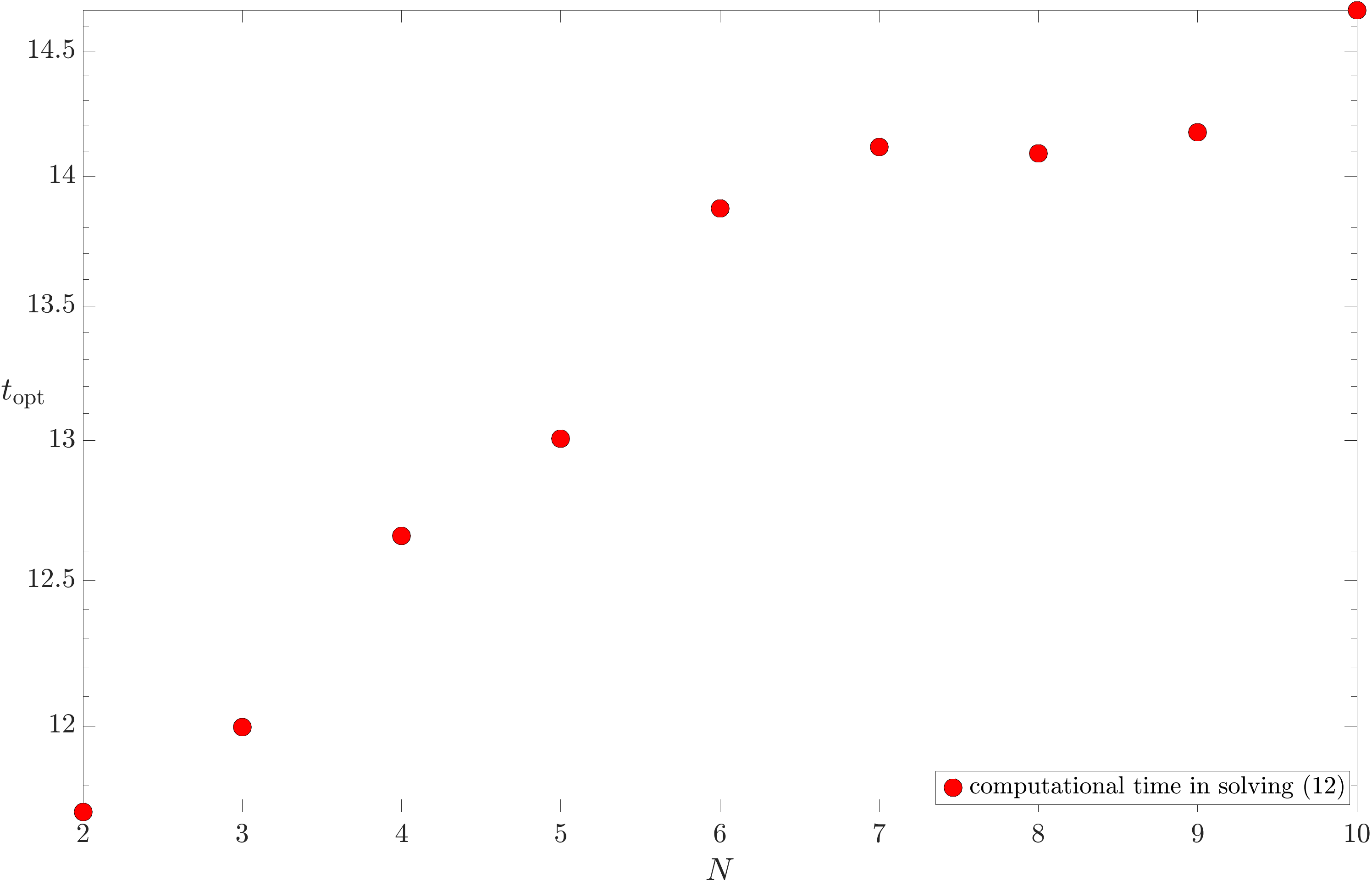
Figure 4. Computational times [s] for solving (12) against $N$.

To design the supervisory algorithm shown in Fig. 1 for adapting $N_{\max}$, we used a fourth degree polynomial regression to estimate $f$ in (15). The corresponding least square estimate is depicted in Fig. 3. Fig. 4 reveals that $t_{\text{opt}}<<t_{\text{propagation}}$ for our simulation, i.e., $t_{\text{total}}$ is dominated by the time needed to solve the IVPs.

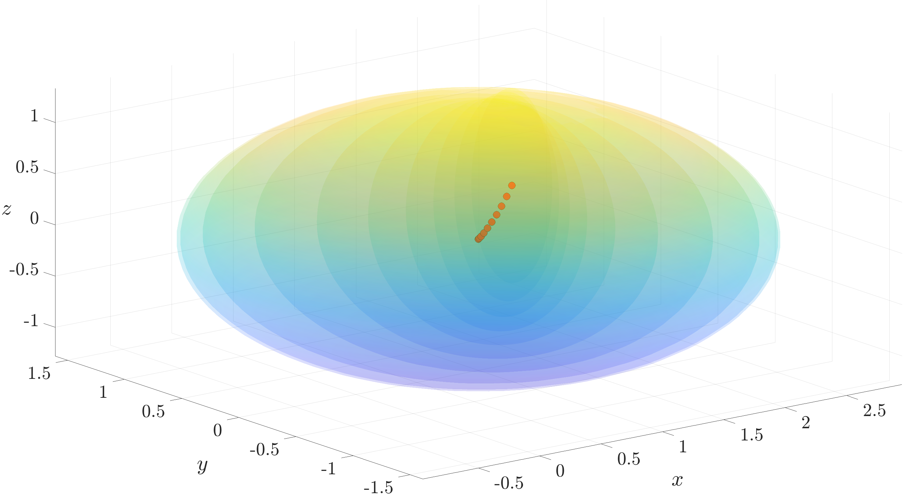
Figure 5. The ellipsoidal outer-approximations of the reach set in $(x,y,z)$ for the simulation case study in Sec. 4 with $N_{\max}=10$. Shown here are 10 equi-spaced time snapshots superimposed for $t\in[0,1]$. The red dots show the centers of the respective ellipsoidal over-approximations.

In Fig. 5, we show the ellipsoidal over-approximations for reach sets in the position coordinates $(x,y,z)$ for $t\in[0,1]$, obtained using the proposed framework.

5. Conclusions and Future Work

We outlined an anytime ellipsoidal over-approximation framework for the forward reach sets of an uncertain linear system with ellipsoidal set-valued uncertainties. Our main intent was to point out that the existing ellipsoidal over-approximation results are well-positioned for anytime implementation, thereby opening up the possibility to deploy them for safety-critical CPS applications in a manner that not only acknowledges the limited computational resource in these settings, but dynamically adapts its performance depending on processor availability without sacrificing safety. We provided a numerical case study to elucidate the ideas.

Several avenues of future work remain open. For example, instead of regression, one may design the supervisory algorithm for computing $N_{\max}$ via online learning. It may also be interesting to analyze the performance of these anytime algorithms under stochastic processor availability models, as was done in control settings (Gupta, 2010; Quevedo et al., 2014; Fontanelli et al., 2008). One may also be interested to design anytime algorithms for other parametric over-approximation algorithms, e.g., using zonotopes (Althoff, 2015).

- (1)
- Althoff (2015) Matthias Althoff. 2015. An Introduction to CORA 2015. Proc. of the Workshop on Applied Verification for Continuous and Hybrid Systems (2015), 120–151.
- Anderson and Moore (2007) Brian DO Anderson and John B Moore. 2007. Optimal control: linear quadratic methods. Courier Corporation.
- Belforte et al. (1990) Gustavo Belforte, Basilio Bona, and Vito Cerone. 1990. Parameter estimation algorithms for a set-membership description of uncertainty. Automatica 26, 5 (1990), 887–898.
- Ben-Tal and Nemirovski (2001) Aharon Ben-Tal and Arkadi Nemirovski. 2001. Lectures on modern convex optimization: analysis, algorithms, and engineering applications. SIAM.
- Bertsekas and Rhodes (1971) Dimetri Bertsekas and Ian Rhodes. 1971. Recursive state estimation for a set-membership description of uncertainty. IEEE Trans. Automat. Control 16, 2 (1971), 117–128.
- Bhattacharya and Balas (2004) Raktim Bhattacharya and Gary J Balas. 2004. Anytime control algorithm: Model reduction approach. Journal of Guidance, Control, and Dynamics 27, 5 (2004), 767–776.
- Boyd et al. (1994) Stephen Boyd, Laurent El Ghaoui, Eric Feron, and Venkataramanan Balakrishnan. 1994. Linear matrix inequalities in system and control theory. SIAM.
- Boyd and Vandenberghe (2004) Stephen Boyd and Lieven Vandenberghe. 2004. Convex optimization. Cambridge university press.
- Chernous’ko (1980) Feliks Leonidovich Chernous’ko. 1980. Guaranteed estimates of undetermined quantities by means of ellipsoids. In Doklady Akademii Nauk, Vol. 251. Russian Academy of Sciences, 51–54.
- Devonport and Arcak (2020a) Alex Devonport and Murat Arcak. 2020a. Data-driven reachable set computation using adaptive Gaussian process classification and Monte Carlo methods. In 2020 American Control Conference (ACC). IEEE, 2629–2634.
- Devonport and Arcak (2020b) Alex Devonport and Murat Arcak. 2020b. Estimating reachable sets with scenario optimization. In Learning for Dynamics and Control. PMLR, 75–84.
- Fan et al. (2017) Chuchu Fan, Bolun Qi, Sayan Mitra, and Mahesh Viswanathan. 2017. DRYVR: data-driven verification and compositional reasoning for automotive systems. In International Conference on Computer Aided Verification. Springer, 441–461.
- Fogel (1979) Eli Fogel. 1979. System identification via membership set constraints with energy constrained noise. IEEE Trans. Automat. Control 24, 5 (1979), 752–758.
- Fontanelli et al. (2008) Daniele Fontanelli, Luca Greco, and Antonio Bicchi. 2008. Anytime control algorithms for embedded real-time systems. In International Workshop on Hybrid Systems: Computation and Control. Springer, 158–171.
- Grötschel et al. (1993) Martin Grötschel, László Lovász, and Alexander Schrijver. 1993. Geometric algorithms and combinatorial optimization. Vol. 2. Springer Science & Business Media.
- Gupta (2010) Vijay Gupta. 2010. On a control algorithm for time-varying processor availability. In Proceedings of the 13th ACM international conference on Hybrid systems: computation and control. 81–90.
- Haddad and Halder (2021) Shadi Haddad and Abhishek Halder. 2021. The Curious Case of Integrator Reach Sets, Part I: Basic Theory. arXiv:eess.SY/2102.11423
- Halder (2018) Abhishek Halder. 2018. On the parameterized computation of minimum volume outer ellipsoid of Minkowski sum of ellipsoids. In 2018 IEEE Conference on Decision and Control (CDC). IEEE, 4040–4045.
- Henk (2012) Martin Henk. 2012. Löwner-John ellipsoids. Documenta Math 95 (2012), 106.
- John (1948) Fritz John. 1948. Extremum Problems with Inequalities as Subsidiary Conditions. Studies and Essays: Courant Anniversary Volume, presented to R. Courant on his 60th Birthday (1948), 187–204.
- Kosut et al. (1992) Robert L Kosut, Ming K Lau, and Stephen P Boyd. 1992. Set-membership identification of systems with parametric and nonparametric uncertainty. IEEE Trans. Automat. Control 37, 7 (1992), 929–941.
- Kurzhanski and Varaiya (2014) Alexander B Kurzhanski and Pravin Varaiya. 2014. Dynamics and Control of Trajectory Tubes: Theory and Computation. Vol. 85. Springer.
- Kurzhanskiĭ and Vályi (1997) Alexander B Kurzhanskiĭ and István Vályi. 1997. Ellipsoidal calculus for estimation and control. Nelson Thornes.
- Kurzhanskiy and Varaiya (2006) Alex A Kurzhanskiy and Pravin Varaiya. 2006. Ellipsoidal toolbox (ET). In Proceedings of the 45th IEEE Conference on Decision and Control. IEEE, 1498–1503.
- Liebenwein et al. (2018) Lucas Liebenwein, Cenk Baykal, Igor Gilitschenski, Sertac Karaman, and Daniela Rus. 2018. Sampling-based approximation algorithms for reachability analysis with provable guarantees. In Robotics: Science and Systems XIV (RSS).
- Mitchell (2008) Ian M Mitchell. 2008. The flexible, extensible and efficient toolbox of level set methods. Journal of Scientific Computing 35, 2 (2008), 300–329.
- Norton (1987) JP Norton. 1987. Identification and application of bounded-parameter models. Automatica 23, 4 (1987), 497–507.
- Pant et al. (2015) Yash Vardhan Pant, Houssam Abbas, Kartik Mohta, Truong X Nghiem, Joseph Devietti, and Rahul Mangharam. 2015. Co-design of anytime computation and robust control. In 2015 IEEE Real-Time Systems Symposium. IEEE, 43–52.
- Pólik and Terlaky (2007) Imre Pólik and Tamás Terlaky. 2007. A survey of the S-lemma. SIAM review 49, 3 (2007), 371–418.
- Quevedo et al. (2014) Daniel E Quevedo, Wann-Jiun Ma, and Vijay Gupta. 2014. Anytime control using input sequences with Markovian processor availability. IEEE Trans. Automat. Control 60, 2 (2014), 515–521.
- Schweppe (1968) Fred Schweppe. 1968. Recursive state estimation: Unknown but bounded errors and system inputs. IEEE Trans. Automat. Control 13, 1 (1968), 22–28.
- Vandenberghe et al. (1998) Lieven Vandenberghe, Stephen Boyd, and Shao-Po Wu. 1998. Determinant maximization with linear matrix inequality constraints. SIAM journal on matrix analysis and applications 19, 2 (1998), 499–533.
- Witsenhausen (1968) HS Witsenhausen. 1968. Sets of possible states of linear systems given perturbed observations. IEEE Trans. Automat. Control 13, 5 (1968), 556–558.
- Yakubovich (1971) VA Yakubovich. 1971. S-procedure in nonlinear control theory. Vestnick Leningrad Univ. Math. (in Russian) (1971), 62–77.
- Yakubovich (1992) VA Yakubovich. 1992. Nonconvex optimization problem: The infinite-horizon linear-quadratic control problem with quadratic constraints. Systems & Control Letters 19, 1 (1992), 13–22.
- Zilberstein (1995) Shlomo Zilberstein. 1995. Operational rationality through compilation of anytime algorithms. AI Magazine 16, 2 (1995), 79–79.
- Zilberstein (1996) Shlomo Zilberstein. 1996. Using anytime algorithms in intelligent systems. AI magazine 17, 3 (1996), 73–73.