A Reinforcement Learning Based R-Tree for Spatial Data Indexing in Dynamic Environments

Abstract.

Learned indices have been proposed to replace classic index structures like B-Tree with machine learning (ML) models. They require to replace both the indices and query processing algorithms currently deployed by the databases, and such a radical departure is likely to encounter challenges and obstacles. In contrast, we propose a fundamentally different way of using ML techniques to improve on the query performance of the classic R-Tree without the need of changing its structure or query processing algorithms. Specifically, we develop reinforcement learning (RL) based models to decide how to choose a subtree for insertion and how to split a node when building an R-Tree, instead of relying on hand-crafted heuristic rules currently used by R-Tree and its variants. Experiments on real and synthetic datasets with up to more than 100 million spatial objects clearly show that our RL based index outperforms R-Tree and its variants in terms of query processing time.

1. Introduction

To support efficient processing of spatial queries, such as range queries and KNN queries, spatial databases have relied on delicate indices. The R-Tree (Guttman, 1984) is arguably the most popular spatial index that prunes irrelevant data for queries. R-Trees have attracted extensive research interests (Beckmann et al., 1990; Sellis et al., 1987; Beckmann and Seeger, 2009; Pavlovic et al., 2018; Ross et al., 2001; Kanth et al., 1997; Kamel and Faloutsos, 1993; Arge et al., 2008; Leutenegger et al., 1997; García R et al., 1998; Roussopoulos and Leifker, 1985; Qi et al., 2018; Wang et al., 2019; Qi et al., 2020; Li et al., 2020; Nathan et al., 2020; Ding et al., 2020b; Davitkova et al., 2020; Yang et al., 2020) and are widely used in commercial databases such as PostgreSQL and MySQL.

The learned index has been proposed in (Kraska et al., 2018), which proposes a recursive model index (RMI) for indexing 1-dimensional data by learning a cumulative distribution function (CDF) to map a search key to a rank in a list of ordered data objects. To address the limitations of the RMI, such as the lack of supporting updates, and to improve it, several learned indices have been proposed based on the RMI. The idea of learned indices is also extended for spatial data (Qi et al., 2020; Wang et al., 2019; Li et al., 2020; Pandey et al., 2020) and multi-dimensional data (Nathan et al., 2020; Ding et al., 2020b; Davitkova et al., 2020). They usually map spatial data points in a dataset to a uniform rank space (e.g., using a space filling curve), and then learn the CDF for this dataset. Despite the success of these learned indices in improving the efficiency of processing some types of queries, they still have various limitations, e.g., they can only handle spatial point objects and limited types of spatial queries, some only return approximate query results, and they either cannot handle updates or need a periodic rebuild to retain high query efficiency (Details in Section 5). These limitations, together with the requirement that the learned indices need a replacement of the index structures and query processing algorithms currently used by spatial database systems, would make them not easy to be deployed in current database systems.

In this work, rather than learning a CDF for spatial data, we consider a fundamentally different approach, i.e., to use machine learning techniques to construct an R-Tree in a data-driven way for better query efficiency in a dynamic environment where updates occur frequently and bulk loading is not viable. Specifically, we propose to build machine learning models for the two key operations of building an R-Tree, namely $\mathsf{ChooseSubtree}$ and $\mathsf{Split}$ operations, which currently rely on hand-crafted heuristic rules. Note that we do not modify the basic structure of the R-Tree and thus all the currently deployed query processing algorithms will still be applicable to our proposed index. This would make it easier for the learning based index to be deployed by current databases.

To motivate our idea, we next revisit $\mathsf{ChooseSubtree}$ and $\mathsf{Split}$. When inserting a new spatial object, the $\mathsf{ChooseSubtree}$ operation is invoked iteratively, i.e., choosing which child node to insert the new data object, until a leaf node is reached. If the number of entries in a node exceeds the capacity, the Split operation is invoked to divide the entries into two groups. Many R-Tree variants have been proposed, which mainly differ in their strategies for the insertion of new objects (i.e., $\mathsf{ChooseSubtree}$) as well as algorithms for splitting a node (i.e., $\mathsf{Split}$). Almost all these strategies are based on hand-crafted heuristics. However, there is no single heuristic strategy that dominates the others in terms of query performance. To illustrate this, we generate a dataset with 1 million uniformly distributed data points and construct four R-Tree variants using four different Split strategies, namely linear (Guttman, 1984), quadratic (Guttman, 1984), Greene’s (Greene, 1989) and R*-Tree (Beckmann et al., 1990). We run 1,000 random range queries and rank the four indices based on the query processing time of each individual query. We observe that no single index has the best performance for all the queries. For example, Greene’s Split has the best query performance among 50% of the queries while R*-Tree Split is the best for 49% of the queries. The observation that no single index dominates the others holds on other datasets as well, and the top performers may be different on different datasets.

The observation motivates us to develop machine learning models to handle the $\mathsf{ChooseSubtree}$ and $\mathsf{Split}$ operations, to replace the heuristic strategies used in the R-Tree and its variants. Furthermore, we observe that the two operations can be considered as two sequential decision making problems. Therefore, we model them as two Markov decision processes (MDPs) (Puterman, 2014) and propose to use reinforcement learning (RL) to learn models for the two operations.

However, it is very challenging to make the idea work—We have tried various ways to define the two MDPs, which significantly affect the performance of the learned models. The first challenge is how to formulate $\mathsf{ChooseSubtree}$ and $\mathsf{Split}$ as MDPs. How should we define the states, actions, and the reward signals for each MDP? Specifically, 1) Designing the action space. A straightforward idea could be to define an action as one of the existing heuristic strategies. However, the idea did not work, for which we observed from the experiments that different strategies would often make the same insertion/splitting decision, and thus it leaves us very little room for improvement. Some other possible ideas include defining larger action spaces, but then it would increase the difficulty of training the model. 2) Designing the state. As the number of entries varies across different R-Tree nodes, it is challenging to represent the state of a node for both operations. 3)  Designing the reward signal. It is nontrivial to design a function that evaluates the reward of past actions during model training to encourage the RL agent to take “good” actions in our problem.

The second challenge is how to use RL to address the defined MDPs. For instance, in the construction of an R-Tree, node overflow (and thus the $\mathsf{Split}$ operation) occurs less frequently than the $\mathsf{ChooseSubtree}$ operation. Therefore, only a few state transitions for Split operations are generated, making it difficult for the RL agent to learn useful information. Moreover, a previous decision ($\mathsf{ChooseSubtree}$ or $\mathsf{Split}$) may affect the structure of the R-Tree in the future. Therefore, a “good” action may receive a bad reward due to some bad actions that were made previously. This makes it even more challenging to learn a good policy to solve the two MDPs.

Our method. To this end, we propose the RL based R-Tree, called RLR-Tree. In the RLR-Tree, we carefully model the two MDPs, $\mathsf{ChooseSubtree}$ and $\mathsf{Split}$, and propose a novel RL-based method to learn policies to solve them. The learned policies replace the hand-crafted heuristic rules to build a different R-Tree, namely RLR-Tree. The RLR-Tree possesses several salient features:

(1) Its models are trained on a small training dataset and then used to build an RLR-Tree on datasets of much larger scales. Furthermore, models trained on one data distribution can be applied to data with a different distribution to build an RLR-Tree, the RLR-Tree still significantly outperforms the R-Tree and its variants in answering spatial queries.

(2) It achieves up to 95% better query performance than the R-Tree and its variants that are designed for a dynamic environment.

(3) Like the R-Tree, the RLR-Tree can be built on spatial objects of different types, such as points or rectangles. However, to the best of our knowledge, existing learned indices (Qi et al., 2020; Nathan et al., 2020; Ding et al., 2020b; Davitkova et al., 2020; Li et al., 2020; Wang et al., 2019) can only handle point objects when used for spatial data.

(4) The RLR-Tree simply deploys any existing query processing algorithms for R-Trees to answer queries of different types, without the need of designing new query processing algorithms. However, other learning based indices (Qi et al., 2020; Nathan et al., 2020; Ding et al., 2020b; Davitkova et al., 2020; Li et al., 2020; Wang et al., 2019) often only focus on limited types of queries, e.g., range queries, and they need to design new algorithms for each type of query.

In summary, we make the following contributions:

(1) We propose to train machine learning models to replace heuristic rules in the construction of an R-Tree to improve on its query efficiency in a dynamic environment where updates occur frequently and bulk loading is not viable. To the best of our knowledge, this is the first work that uses machine learning to improve on the R-Tree without modifying its structure; Therefore, all currently deployed query processing algorithms are still applicable and the proposed index can be easily deployed by current databases.

(2) We model the $\mathsf{ChooseSubtree}$ and the $\mathsf{Split}$ operations as two MDPs, and carefully design their states, actions and reward signals. We also present some of our unsuccessful trials of designing.

(3) We design an effective and efficient learning process that learns good policies to solve the MDPs. The learning process enables us to apply our RL models trained with a small dataset to build an R-Tree for up to more than 100 million spatial objects.

(4) We conduct extensive experiments on both real and synthetic datasets. The experimental results show that our proposed index achieves up to 95% better query performance for range queries and 96% for KNN queries than R-Tree and its variants, and up to 40% better query performance for range queries and 42% for KNN queries than LISA (Li et al., 2020), which is the only disk based learned spatial index that returns exact results for range queries and KNN queries.

2. Preliminary and Problem

2.1. Preliminary

R-Tree (Guttman, 1984) is a balanced tree for indexing multi-dimensional objects, such as coordinates and rectangles. Each tree node can contain at most $M$ entries. Each node (except the root node) must also contain at least $m$ entries. Each entry in a non-leaf node consists of a reference to a child node and the minimum bounding rectangle (MBR) of all entries within this child node. Each leaf node contains entries, each of which consists of a reference to an object and the MBR of that object. Therefore, a query that does not intersect with the MBR cannot intersect any of the contained objects.

The algorithms for building an R-Tree comprise two key operations, ChooseSubtree and Split. To insert an object into an R-Tree, starting from the root node, $\mathsf{ChooseSubtree}$ is iteratively invoked to decide in which subtree to insert the object, until a leaf node is reached. The object is inserted into the leaf node and its corresponding MBR is updated accordingly. If the number of entries in a leaf node exceeds $M$, the $\mathsf{Split}$ operation is invoked to divide the objects into two groups: one remains in the original leaf node and the other will become a new leaf node. The Split operation may be propagated upwards as an entry referring to the new leaf node is added to its parent node, which may overflow and need to be split.

The query performance of an R-Tree highly depends on how the R-Tree is built. Many R-Tree variants have been proposed with different $\mathsf{ChooseSubtree}$ and $\mathsf{Split}$ strategies as discussed in Section 1.

2.2. Problem Statement

As discussed in Section 1, most of the existing R-Tree variants adopt hand-crafted $\mathsf{ChooseSubtree}$ and $\mathsf{Split}$ strategies, and no strategy can build an R-Tree with dominant query performance in all cases. Motivated by this, we aim to learn to build an R-Tree, i.e., using RL models to make decisions for $\mathsf{ChooseSubtree}$ and $\mathsf{Split}$ instead of relying on heuristic rules. The new index is called RLR-Tree.

3. RLR-Tree

3.1. Overview

The process of inserting a new object into an R-Tree is essentially a combination of two typical sequential decision making processes. In particular, starting from the root, it needs to make a decision on which child node to insert the new object at each level in a top-down traversal ($\mathsf{ChooseSubtree}$). It also needs to make a decision on how to split an overflowing node and divide the entries in a bottom-up traversal ($\mathsf{Split}$). Reinforcement learning (RL) has been proven to be effective in solving sequential decision making problems. Therefore, we propose to model the insertion of a new object as a combination of two Markov decision processes (MDPs) and adopt RL to learn the optimal policies for $\mathsf{ChooseSubtree}$ and $\mathsf{Split}$ operations.

Figure 1 depicts an overview of the proposed solution to build an RLR-Tree, as well as using the RLR-Tree to answer queries. In offline training, we propose new solutions to train RL $\mathsf{ChooseSubtree}$ and RL $\mathsf{Split}$ models using a small dataset or a subset. This is the focus of this work. Note that models trained on one dataset is readily applied on a different dataset as shown in experiments. The two trained models can be integrated into the algorithms for R-Tree construction to build the RLR-Tree and R-tree maintenance with dynamic updatets. Finally, any existing query processing algorithm designed for the R-Tree family can be used for RLR-Tree to answer different types of spatial queries.

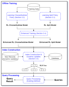
Figure 1. RLR-Tree Overview

Next, we focus on the offline training and present our final designs for the two MDPs and the other representative designs that we have explored to formulate the problem. We present RL $\mathsf{ChooseSubtree}$ and its model training in Section 3.2, and RL $\mathsf{Split}$ and its model training in Section 3.3. We present how to train the two models together in Section 3.4. We briefly introduce how to integrate the trained models into existing algorithms to construct the RLR-Tree and then to handle updates in Section 3.5.

3.2. ChooseSubtree

To insert a new object into the R-Tree, we need to conduct a top-down traversal starting from the root. In each node, we need to decide which child node to insert the new object. To choose a subtree with RL, we formulate this problem as an MDP. We proceed to present how to train a model to learn a policy for the MDP.

3.2.1. MDP Formulation

An MDP consists of four components, namely states, actions, transitions, and rewards. We proceed to explain how states and actions are represented in our model, and then present the reward signal design, which is particularly challenging.

MDP: State Space. A state captures the environment that is taken into account for decision making. For $\mathsf{ChooseSubtree}$, it is a natural idea that a state is from the tree node whose child nodes are to be selected for inserting a new object. The challenging question is: what kind of information should we extract from the tree node to represent the state?

Intuitively, as we need to decide which child node to insert the new object, it is necessary to incorporate the change of the child node if we add the new object into it for each child node. Possible features that capture the change of a child node $N$ include: (1) $\Delta Area(N,o)$, which is the area increase of the MBR of $N$ if we add the new object $o$ into $N$; (2) $\Delta Peri(N,o)$, which is the perimeter increase of the MBR of $N$ if we add $o$ into $N$, and (3) $\Delta Ovlp(N,o)$, which is the increase of the overlap between $N$ and other child nodes after $o$ is inserted into $N$. Furthermore, it is helpful to know the occupancy rate of the child node, denoted by $OR(N)$, which is the ratio of the number of entries to the capacity. A child node with a high occupancy rate is more likely to overflow in the future.

As we have presented several features to capture the properties of a tree node, a straightforward idea is that we compute the aforementioned features for every child node and concatenate them to represent the state. However, the number of child nodes varies across different nodes, making it difficult to represent a state with a vector of a fixed length. An idea to address this challenge is to do padding, i.e., to append zeros to the features of the child nodes to get a $4\cdotp M$ dimensional vector, as there are four features and there are at most $M$ child nodes. However, the padded representations are likely to have many zeros which will add noises and mislead the model, resulting in poor performance. This is confirmed by our preliminary experiments.

To address the challenge, we propose to only use a small part of child nodes to define the state. This is because most of the child nodes are not good candidates for hosting the new object, as inserting the new object may greatly increase their MBRs. Here we aim to prune unpromising child nodes from the state space, and our RL agent will not consider them for representing a state. Our design of state representation is as follows: We first retrieve the top-$k$ child nodes in ascending order of area increase, where the choice of area increase is based on empirical findings. Then for each retrieved child node, we compute four features $\Delta Area(N,o)$, $\Delta Peri(N,o)$, $\Delta Ovlp(N,o)$, and $OR(N)$. We concatenate the features of the $k$ child nodes to get a $4\cdotp k$ dimensional vector to represent a state. $k$ is a parameter to be set empirically. Note that to make the representation of different states comparable, the increases of area, perimeter and overlap are normalized by the maximum corresponding value among all $k$ child nodes.

Remark. It is a natural idea that we can include more features to represent a state. For instance, we can include global information, such as the tree depth and the size of the tree, and local information, such as the depth of the tree node, the coordinates of the boundary of the MBR. However, our experiments show that these features do not improve the performance of our model while making the model training slower. The four features that we use are sufficient to train our model to make good subtree choices as shown in our experiments. It would be a useful future direction to design and evaluate other state features.

MDP: Action Space. As many R-Tree variants have been proposed with different $\mathsf{ChooseSubtree}$ strategies, such as minimizing the increase of area, perimeter, or overlap. A straightforward idea is to make the different cost functions the actions, i.e., to decide which cost function to use to choose the subtree. After trying different combinations of these cost functions and different state space designs, this idea is proven to be ineffective by our experimental results. Table 1 depicts the average relative I/O cost for processing 1,000 random range queries on three datasets of different distributions, namely Skew, Gaussian and Uniform. The relative I/O cost will be defined in Section 4.1. Intuitively, if the relative I/O cost is smaller than 1, the index requires fewer nodes accesses than the R-Tree does. We observe from Table 1 that compared with the R-Tree, an RL model with the cost functions as actions only achieves an improvement of less than 2% in terms of query processing time. We find from our experiments that in 90% of the nodes, different cost functions end up with the same subtree choice which gives us very little room for improvement.

Table 1. Performance of cost function based action space.

	Relative I/O cost
	Skew	Gaussian	Uniform
Use cost functions	0.98	0.98	1.00
Our final design	0.29	0.08	0.56

As a result, we propose a new idea of training the RL agent to decide which child node to insert the new object directly. Based on the idea, one design is to have all child nodes to comprise the action space. However, this incurs two challenges: 1) the number of child nodes contained by different nodes is usually different, and 2) the action space is large. Considering all child nodes as the actions leads to a large action space with many “bad actions”. The bad actions make the exploration during model training ineffective and inefficient. To address the challenges, we use the similar idea as we use for designing state space. Recall that in designing the state space, we propose to retrieve top-$k$ child nodes in terms of the increase of area to represent a state. To make the action space and the state representation consistent, we define the action space $\mathcal{A}=\{1,\dots,k\}$, where action $a=i$ means the RL agent chooses the $i$-th retrieved child node to be inserted with the new object.

MDP: Transition. In the process of the $\mathsf{ChooseSubtree}$ operation, given a state (a node in the R-Tree) and an action (inserting the new object into a child node), the RL agent transits to the child node. If the child node is a leaf node, the agent reaches a terminal state.

MDP: Reward Signal. A reward associated with a transition corresponds to some feedback indicating the quality of the action taken at a given state. A larger reward indicates a better quality. Since our objective is to learn to build an R-Tree that processes query efficiently, the reward signal is expected to reflect the improvement of query performance.

In the process of $\mathsf{ChooseSubtree}$, it is challenging to directly evaluate if an action taken at a state is good, because the new object has not been fully inserted into the tree yet. A straightforward idea is after the new object has been inserted, we use the R-Tree to process a set of random range queries. The inverse of the cost (e.g., the number of accessed nodes) for processing the queries is set as the reward shared by all of the state-action pairs encountered in the insertion of the new object. The agent seems to be encouraged to take the actions to build a tree that can process range queries by accessing as few nodes as possible. However, this is not the case due to the following reasons: (1) A previous action may affect the tree structure and hence the query performance in the future. Therefore, a “good” action may receive a poor reward due to some bad actions that were made previously. (2) More importantly, as we aim to learn to construct an R-Tree that outperforms the competitors, we are interested in knowing what kind of actions makes the resulting tree better than a competitor, and what kind of actions makes it worse. The aforementioned reward signal cannot distinguish the two types of actions, making it ineffective for the agent to learn a good policy to outperform the competitors. (3) As more objects are inserted into the R-Tree, the average number of accessed nodes naturally increases. Therefore, the reward signal becomes weaker and weaker, which makes it difficult for the model to learn useful information in the late stage of the training.

Inspired by the observations, we design a novel reward signal for $\mathsf{ChooseSubtree}$. The high level idea is that we maintain a reference tree with a fixed $\mathsf{ChooseSubtree}$ and $\mathsf{Split}$ strategy. The reference tree serves as a competitor and can be any existing R-Tree variant. The reward signal is computed based on the gap between costs for processing random queries with the reference tree and the RLR-Tree. Specifically, the design of the reward signal is as follows:

(1) We maintain an R-Tree, namely RLR-Tree, that uses RL to decide which child node to insert the new object, and adopts a pre-specified Split strategy.

(2) We maintain a reference tree which adopts a pre-specified $\mathsf{ChooseSubtree}$ strategy and the same Split strategy as RLR-Tree.

(3) We synchronize the reference tree with the RLR-Tree, so that they have the same tree structure.

(4) Given $p$ new objects $\{o_{1},\dots,o_{p}\}$, we insert them into both the reference tree and the RLR-Tree.

(5) After the $p$ objects are inserted, we generate $p$ range queries of predifined sizes whose centers are at the $p$ objects, respectively.

(6) The $p$ range queries are processed with both the reference tree and the RLR-Tree. We compute the normalized node access rate, which is defined as $\frac{\text{\# acc. nodes}}{\text{Tree height}}$ and is the number of accessed nodes for answering a range query over the tree height. Let $R$ and $R^{\prime}$ be the normalized node access rate of the RLR-Tree and the reference tree, respectively. We compute $r=R^{\prime}-R$ as the reward signal. The higher $r$ is, the fewer nodes RLR-Tree needs to access to process the range queries than the reference tree.

(7) All the transitions encountered in the insertion of the $p$ objects share the same reward $r$.

With the idea, we are able to distinguish the good actions from the bad actions: A positive reward means that the RLR-Tree processes the recent $p$ insertions well as it requires fewer nodes accesses to process the queries compared with the reference tree. Moreover, as the reference tree is periodically synchronized with the RLR-Tree, we can avoid the effect of previous actions. Therefore, maximizing the accumulated reward is equivalent to encouraging the agent to take the actions that can make the RLR-Tree outperform the competitors.

3.2.2. Training the Agent for $\mathsf{ChooseSubtree}$

Deep-$Q$-Network (DQN) Learning. Deep Q-learning is a commonly used model-free RL method. It uses a Q-function $Q^{*}(s,a)$ to represent the expected accumulated reward that the agent can obtain if it takes action $a$ in state $s$ and then follows the optimal policy until it reaches a terminal state. The optimal policy takes the action with the maximum $Q$-value in any state. Deep-$Q$-Network (Mnih et al., 2015) has been proposed to approximate the Q-function $Q^{*}(s,a)$ with a deep neural network $Q(s,a;\Theta)$ with parameters $\Theta$. In our model, we adopt the deep Q-learning with experience replay (Mnih et al., 2015) for learning the $Q$-functions.

Given a batch of transitions $(s,a,r,s^{\prime})$, parameters in $Q(s,a;\Theta)$ is updated with a gradient descent step by minimizing the mean square error (MSE) loss function, as shown in Equation 1.

(1) $$\vspace*{-2mm}L(\theta)=\sum_{s,a,r,s^{\prime}}[(r+\gamma max_{a^{\prime}}\hat{Q}(s^{\prime},a^{\prime};\Theta^{-})-Q(s,a;\Theta))^{2}],$$

where $\gamma$ is the discount rate, and $\hat{Q}(;\Theta^{-})$ is frozen target network.

Training the Agent. We present the RL $\mathsf{ChooseSubtree}$ training process in Algorithm 1. We first initialize the main network $Q(s,a;\Theta)$ and the target network $\hat{Q}(s,a;\Theta^{-})$ with the same random weights (line 3). In each epoch, it first resets the replay memory (line 5). Then it involves a sequence of insertions of the objects in the training dataset (lines 6–20). Specifically, for every $p$ objects $\{o_{1},\dots,o_{p}\}$, we synchronize the structure of $T_{r}$ with $T_{rl}$ (line 7). For each $o_{i}$ of the $p$ objects, we first insert it into the reference tree (line 9). Then a top-down traversal on the RLR-Tree is conducted (lines 10–15). At each level, we compute the state representation (line 12) and use $\epsilon$-greedy to choose the action based on their $Q$-values (line 13), until we reach a terminal state (leaf node). The transitions are stored in $SA$ (line 14). At the leaf node, we insert the new object and use the same $\mathsf{Split}$ strategy as the reference tree in a bottom-up scan to ensure no node overflows (line 15). Meanwhile, we generate a range query with a predefined size centered at $o_{i}$ and add the query to $RQ$ (line 16). When the $p$ objects have been inserted, we compute the reward with the queries in $RQ$ (line 17). The reward computation process is illustrated in Figure 2. All transitions encountered in the insertions of the $p$ objects share the same reward $r$ and are pushed into the replay memory (line 18). Then we draw a batch of transitions randomly from the replay memory and use the batch to update the parameters in the main network $Q(;\Theta)$ as DQN does (line 19). The parameters in the target network $\hat{Q}$ are periodically synchronized with $Q$ (line 20).

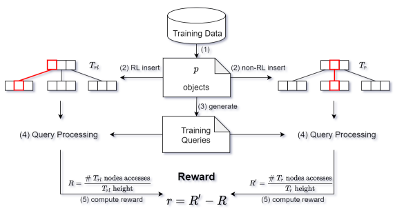
Figure 2. RL $\mathsf{ChooseSubtree}$ Reward Computation

Remark. The new object to be inserted may be fully contained in one of the child nodes. If we add the new object into such a child node, the MBRs of all child nodes are not affected. Therefore, it is unnecessary to make the agent consider such cases. When such cases happen, we do not pass the state representation to the model, but choose the child node that contains the new object directly.

1 Input: A training dataset;

2 Output: Learned action-value function $Q(s,a;\Theta)$;

3 Initialize $Q(s,a;\Theta)$, $\hat{Q}(s,a;\Theta^{-})$;

4 for $epoch=1,2,\dots$ do

5       Replay memory $\mathcal{M}\leftarrow\emptyset$;

6       for every $p$ objects $\{o_{1},\dots,o_{p}\}$ in dataset do

7             $T_{r}\leftarrow T_{rl}$, $SA\leftarrow\emptyset$, $RQ\leftarrow\emptyset$;

8             for $o_{i}\in\{o_{1},\dots,o_{p}\}$ do

9                   Insert $o_{i}$ into $T_{r}$;

10                   $N\leftarrow$ the root of $T_{rl}$;

11                   while $N$ is non-leaf do

12                         $s\leftarrow$ state representation of $N$ and $o_{i}$;

13                         $a\leftarrow$ an action selected by $\epsilon$-greedy based on $Q$-values;

14                         $N\leftarrow a$, $SA\leftarrow SA\cup\{(s,a)\}$;

15                        

16                  Insert $o_{i}$ into $N$, split until no node overflows;

17                   $RQ\leftarrow RQ\cup\{\text{a range query centered at }o_{i}\}$;

18                  

19            $r\leftarrow$ compute reward with queries in $RQ$;

20             Add $(s,a,r,s^{\prime})$ for every $(s,a)\in SA$ into memory;

21             Draw samples from memory and update $\Theta$ in $Q(;\Theta)$;

22             Periodically synchronize $\hat{Q}(;\Theta^{-})$ with $Q(;\Theta)$;

23            

Algorithm 1 DQN Learning for $\mathsf{ChooseSubtree}$

3.2.3. Time Complexity

In our analysis, the additional computation cost associated with the use of neural networks in an RLR-Tree is deemed constant. Assume the RLR-Tree has a size of $S$ and a height of $h$. Inserting an object into the RLR-Tree encounters $h-1$ states. At each state, it takes $O(k\cdot M)$ time to retrieve the top-$k$ child nodes and $O(M)$ to compute the features for each child node. Therefore, the overall time complexity is $O(h\cdotp k\cdot M)$. As a comparison, it takes $O(h\cdotp M)$ time for $\mathsf{ChooseSubtree}$ in the R-Tree.

3.3. Split

The top-down traversal ends up at a leaf node. If the leaf node overflows, it will be split into two nodes and the $\mathsf{Split}$ operation may be propagated upwards. Next, we present how to model $\mathsf{Split}$ as an MDP and how to train the model.

3.3.1. MDP Formulation

We have also explored different ideas to design the state, action, transition and reward signal of the MDP for $\mathsf{Split}$. Due to space limitation, we only present the final design here.

MDP: State Space. For $\mathsf{Split}$, it is natural that a state comes from an overflowing node. A straightforward idea is to make the representation of a state capture the goodness of all the possible splits, so that the agent can decide how to split the node. However, since an overflowing node contains $M+1$ entries, there are $(2^{M+1}-2)$ possible splits in total. It is impractical to reflect all of these splits in the state representation.

In order to avoid considering so many possible splits, we adopt a similar idea as R^∗-Tree (Beckmann and Seeger, 2009) as follows: We first sort the entries with respect to their projection to each dimension. For each sorted sequence, we consider the split at the $i$-th element ($m\leq i\leq M+1-m$), where the first $i$ entries are assigned to the first group and the remaining $M+1-i$ entries are assigned to the second group. This means for each sorted sequence, we only consider $M+2-2\cdot m$ splits. Next, we further discard the splits which create two nodes that overlap with each other. We pick the top-$k$ splits from the remaining splits in ascending order of total area and construct the representation of the state. Specifically, for each split, we consider four features: the areas and the perimeters of the two nodes created by the split. We concatenate the features of all $k$ splits and generate a $4k$-dimensional vector to represent the state. Note that the areas and perimeters are normalized by the maximum area and perimeter among all splits, so that each dimension of the state representation falls in $(0,1]$.

MDP: Action Space. Similar to $\mathsf{ChooseSubtree}$, in order to make the action space consistent with the candidate splits that are used to represent the state, we define the action space as $\mathcal{A}=\{1,\dots,k\}$, where $k$ is the number of splits used to represent the state. An action $a=i$ means that the $i$-th split is adopted.

MDP: Transitions. In $\mathsf{Split}$, given a state (a node in the R-Tree) and an action (a possible split), the agent transits to the state that represents the parent of the node. If the node does not overflow, it is the terminal state.

MDP: Reward Signal. The reward signal for $\mathsf{Split}$ is similar to that of $\mathsf{ChooseSubtree}$. We maintain a reference tree that is periodically synchronized with the RLR-Tree. We use the difference of the normalized node access rate as the two trees process training queries as the reward signal. Note that the RLR-Tree adopts the same $\mathsf{ChooseSubtree}$ strategy as the reference tree and uses the RL agent to decide how to split an overflowing node.

1 Input: A training dataset;

2 Output: Learned action-value function $Q(s,a;\Theta)$;

3

4Initialize $Q(s,a;\Theta)$, $\hat{Q}(s,a;\Theta^{-})$;

5 for $epoch=1,2,3,...$ do

6       for $j=1,2,3,...(parts-1)$ do

7             training part $\leftarrow\emptyset$;

8             Construct $T_{base}$ with the first $\frac{j}{parts}$ of the objects (initial part);

9             for $o$ in the remaining objects do

10                   if Inserting $o$ into $T_{base}$ causes a split then Add $o$ to training part;

11                   else Add $o$ to fill part and insert into $T_{base}$;

12                  

13            for every $p$ objects $\{o_{1},\dots,o_{p}\}\subseteq$ training part do

14                   $T_{rl}\leftarrow T_{base}$, $T_{r}\leftarrow T_{base}$, $SA\leftarrow\emptyset$, $RQ\leftarrow\emptyset$;

15                   for $o_{i}\in\{o_{1},\dots,o_{p}\}$ do

16                         Insert $o_{i}$ into $T_{r}$;

17                         Top-down traversal on $T_{rl}$ to a leaf node $N$;

18                         if $N$ overflows then $RQ\leftarrow RQ\cup\{\text{training query}\}$;

19                         while $N$ overflows do

20                               $s\leftarrow$ state representation of $N$;

21                               $a\leftarrow$ an action selected by $\epsilon$-greedy based $Q$-values;

22                               $N\leftarrow N$’s parent, $SA\leftarrow SA\cup\{(s,a)\}$

23                  $r\leftarrow$ compute reward with queries in $RQ$;

24                   Add $(s,a,r,s^{\prime})$ for all $(s,a)\in SA$ to memory;

25                   Draw samples from memory and update $Q(;\Theta)$;

26                   Periodically synchronize $\hat{Q}(;\Theta^{-})$ with $Q(;\Theta)$;

27                  

Algorithm 2 DQN Learning for $\mathsf{Split}$

3.3.2. Training the Agent for Split

Compared with $\mathsf{ChooseSubtree}$, training the agent for $\mathsf{Split}$ is a more challenging task. To insert an object into the R-Tree, $\mathsf{ChooseSubtree}$ is iteratively invoked at each level in the top-down traversal. On the other hand, $\mathsf{Split}$ operation is invoked only when a node overflows. Therefore, only a few transitions for $\mathsf{Split}$ are available for training, making it difficult for the agent to learn a good policy in reasonable time.

To tackle this challenge, we design a new method for the agent to interact with the environment, so that $\mathsf{Split}$ operation is frequently invoked. Theoretically, if all the nodes are full, the insertion of a new object definitely causes a tree node to split. Inspired by this, we propose to first build a tree in which most of the nodes are full, so that node splits can be frequently encountered. We generate such R-Trees with different sizes, and use the transitions caused by inserting the remaining objects in the dataset for training.

The procedure is presented in Algorithm 2. In each epoch, we repeat $parts-1$ iterations to train the agent (lines 5–24). In particular, in the $i$-th iteration, the first $\frac{i}{parts}$ of the training dataset forms the initial part which is used to construct an R-Tree $T_{base}$ (line 7). The remaining data are then divided into 2 parts, i.e., the fill part containing objects that will not cause node overflow in $T_{base}$ and the training part containing objects not in the fill part. Objects in the fill part are inserted into $T_{base}$ while objects in the training part will be used to trigger splits for training later (line 9–10). In this way, most of the nodes in $T_{base}$ are likely to be full and the objects in the training part are likely to cause splits. This pre-training preparation process is illustrated in Figure 3. After $T_{base}$ is constructed, we start training with objects in the training part (lines 11–24). For every $p$ objects, we first synchronize $T_{r}$ and $T_{rl}$ with $T_{base}$ (line 12). This makes $T_{r}$ and $T_{rl}$ have the same structure and are almost full. Then for each of the $p$ objects, we insert it into the reference tree $T_{r}$ directly with pre-specified $\mathsf{ChooseSubtree}$ and $\mathsf{Split}$ strategies (line 14). For the RLR-Tree, we use the same $\mathsf{ChooseSubtree}$ strategy as the reference tree to reach a leaf node $N$ (line 15). If $N$ overflows, we generate a range query with a predefined size centered at $o_{i}$ and add the query to $RQ$ (line 16). Then we iteratively split $N$ and move to its parent until $N$ does not overflow (lines 17–20). For each node $N$, we compute the state representation and use $\epsilon$-greedy to select an action based on their $Q$-values (lines 18–19). The transitions are stored in $SA$ (line 20). When the $p$ objects have been processed, we compute the reward with the queries in $RQ$ (line 21). The transitions encountered in processing the $p$ objects share the same reward (line 22). Then we draw a batch of random transitions from the replay memory and use it to update the parameters in the main network (line 23). The parameters in the target network $\hat{Q}(;\Theta^{-})$ are periodically synchronized with the main network $Q(;\Theta)$ (line 24).

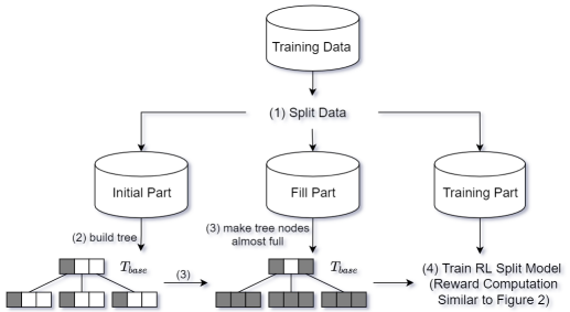
Figure 3. RL $\mathsf{Split}$ Pre-Training Preparation

Remark. When we split a node to two, the ideal case is that the two nodes do not overlap with each other, so that the number of node accesses for processing a query can be reduced. It is more challenging when there are many candidate splits that generate two nodes with zero overlap, as we need to carefully consider how to break the tie. As a result, we consider such a special case in the exploration of the agent. Specifically, if there exists at most one candidate split that generates two non-overlapping nodes, we simply select the split with the minimum overlap. We only use RL to decide how to split the node when more than one split generates non-overlapping nodes. In this way, the agent is trained more effectively.

The training process for $\mathsf{Split}$ has two advantages. Firstly, using different fractions of objects to build an “almost-full” base tree helps to learn a more general model. Secondly, by building the “almost-full” base tree and periodically resetting $T_{r}$ and $T_{rl}$ to the base tree ensures that the $\mathsf{Split}$ operation is consistently invoked at a high frequency. This makes the training process more efficient.

3.3.3. Time Complexity

Similar to $\mathsf{ChooseSubtree}$, the additional computation cost associated with the use of neural networks is deemed constant. If a node overflows, at most $O(h)$ Split operations are invoked. In each Split operation, we first sort the entries along each dimension, which takes $O(M\log M)$ time. Then it takes $O(k\cdotp(M-2m)\cdotp M)$ time to retrieve the top $k$ splits with minimum total area. Finally, it takes $O(k\cdotp M)$ time to compute the four features for the $k$ splits. Therefore, the overall time complexity for RLR-Tree $\mathsf{Split}$ is $O(h\cdotp k\cdotp(M-2m)\cdotp M)$. As a comparison, $\mathsf{Split}$ operation takes $O(h\cdotp M^{2})$ time in the classic R-Tree.

3.4. The Combined Model

We expect that the two agents are closely tied together and are able to help each other achieve better performance. A possible idea for combing the two models is to make the agents share information such as the states observed and the corresponding actions selected with each other. Since both RL models have the same goal, this kind of information sharing has the potential to enhance the agents’ policy learning. However, it is difficult for the two models to exchange information, as they are dealing with different procedures. This approach does not lead to any query performance improvement in the final RLR-Tree.

Recall that we specially design a learning process of Split, as node overflow occurs infrequently in the construction of an R-Tree. Motivated by this, we propose an enhanced training process to train the two agents alternately. Specifically, in odd epochs, we train the RL agent for $\mathsf{ChooseSubtree}$ and the agent for $\mathsf{Split}$ is fixed to be the $\mathsf{Split}$ strategy for the RLR-Tree. In even epochs, we train the agent for $\mathsf{Split}$ and the agent for $\mathsf{ChooseSubtree}$ is fixed to be the $\mathsf{ChooseSubtree}$ strategy for RLR-Tree.

3.5. RLR-Tree Construction & Dynamic Updates

With the learned models for $\mathsf{ChooseSubtree}$ and $\mathsf{Split}$, we incorporate the models into the insertion algorithm of R-Tree to build the RLR-Tree as follows. For each object to be inserted, in the top-down traversal, we iteratively compute the state representation of a node and use the model trained for $\mathsf{ChooseSubtree}$ to select the subtree corresponding to the action with the maximum $Q$-value until the object is inserted into a leaf node. When a node overflows, we compute its state representation and use the model trained for $\mathsf{Split}$ to choose the split corresponding to the action with the maximum $Q$-value. For dynamic updates, new data records can be inserted into an existing tree using the trained models. Our experimental results (Section 4.2.4) show that the trained models do not experience obvious performance deterioration even when there is a change in data distribution.

4. Experiments

4.1. Experimental Setup

Datasets. We use 3 synthetic datasets (1-3) used in previous work on spatial indices (Arge et al., 2008; Qi et al., 2018, 2020), and 2 large real-life datasets (4-5).

1. Skew (SKE): It consists of small squares of a fixed size. The $x$ and $y$ coordinates of the squares centers are randomly generated from a uniform distribution in the range $[0,1]$ and then “squeezed” in the $y$-dimension, that is, each square center $(x,y)$ is replaced by $(x,y^{c})$ where $c$ is the skewness and the default value of which is set to be 9;

2. Gaussian (GAU): It consists of small squares of a fixed size. The coordinates of the center of a square are $(x,y)$ where $x$ and $y$ are randomly generated from a Gaussian distribution with mean $\mu=0.5$ and standard deviation $\sigma=0.2$;

3. Uniform (UNI): It consists of small squares of a fixed size. The $x$ and $y$ coordinates of the centers of the squares are randomly generated from a uniform distribution in the range $[0,1]$;

4. OSM China (CHI): It contains more than 98 million locations in China extracted from OpenStreetMap;

5. OSM India (IND): It contains more than 100 million locations in India extracted from OpenStreetMap.

Note that the centers of all spatial data objects in synthetic datasets fall within the unit square.

Queries. For model training, we run range queries over both the reference R-Tree and the RLR-Tree. Range queries of different sizes are generated. When a range query is generated, we first set its center the same as the center of the last inserted object. Its length to width ratio is then randomly selected in the range $[0.1,10]$. To compare the query performance of RLR-Tree with others, we randomly generate 1,000 range queries for each query size ranging from 0.005% to 2% of the whole region. The testing queries sizes follow the setting in previous work (Qi et al., 2018). Note that queries used for training and testing are generated separately and hence different.

Baselines. We compare with R-Tree and its variants that are designed for dynamic environments where updates occur frequently. Baselines used in the experiments include R-Tree (Guttman, 1984), which is also the reference tree used for model training, R*-Tree (Beckmann et al., 1990), RR*-Tree (Beckmann and Seeger, 2009) which is reported to have the best query performance among R-Tree variants built using one-by-one insertion for supporting queries in dynamic environments. We also compare with LISA (Li et al., 2020) which is the only disk based learned index that returns exact results for range queries and KNN queries. Note that LISA only supports point data, so it is tested on CHI and IND datasets only. We do not compare with packing R-Trees that are designed for the static databases (Kamel and Faloutsos, 1993) or other learned indices as they are not designed for dynamic environments as discussed in Section 5.

Measurements. For measurements of query performance, we consider both running time and the I/O cost. We find that both measures yield qualitatively consistent results (as exemplified in Figure 5). We follow (Li et al., 2020) to report the average relative I/O cost mainly. For each query, the relative I/O cost of an index is computed by the ratio of the I/O cost for it to answer the query to the I/O cost for an R-Tree to answer the same query. Smaller relative I/O costs indicate better query performance compared with the R-Tree.

Parameter settings. Table 2 shows a list of parameters and their corresponding values tested in our experiments. The default settings are bold. For all R-Tree variants evaluated in this paper, we maintain a maximum of 50 and a minimum of 20 child nodes per tree node.

Table 2. Parameters and Values

Parameters	Values
Data distribution	SKE, GAU, UNI
Dataset size (million)	1, 5, 10, 20, 100
Training set size (thousand)	25, 50, 100, 200
Training query size (%)	0.005, 0.01, 2
Testing query size (%)	0.005, 0.01, 0.05, 0.1, 0.5, 1, 2
Action space size $k$	2, 3, 5, 10
Number of dimensions	2, 4, 6, 8, 10

The DQN models for both $\mathsf{ChooseSubtree}$ and $\mathsf{Split}$ contain 1 hidden layer of 64 neurons with SELU (Klambauer et al., 2017) as the activation function. In the training process, the learning rate is set to be 0.003 for RL $\mathsf{ChooseSubtree}$ and 0.01 for RL $\mathsf{Split}$. The initial value of $\epsilon$ is set to be 1 and the decay rate is set to be 0.99. The value of $\epsilon$ is never allowed to be less than 0.1 in order to maintain a certain degree of exploration throughout model training. The replay memory can contain at most 5,000 $(s,a,r,s^{\prime})$ tuples. Network update is done by first sampling a batch of 64 tuples from the replay memory. Then $\Theta$ is updated by using gradient descent of the MSE loss function to close the gap between the Q-value predicted by $\Theta$ and the optimal Q-value derived from $\Theta^{-}$. The discount factor is set to be 0.95 for RL $\mathsf{ChooseSubtree}$ and 0.8 for RL $\mathsf{Split}$. Synchronization of $\Theta^{-}$ with $\Theta$ is done once every 30 network updates.

During the model training for RL $\mathsf{ChooseSubtree}$ (resp. RL $\mathsf{Split}$), the deterministic splitting (resp. insertion) rules are set to be the same as that used by the reference tree which is minimum overlap partition (resp. minimum node area enlargement). We train the RL $\mathsf{ChooseSubtree}$ and $\mathsf{Split}$ models for 20 and 15 epochs, respectively, and set $parts$ in Algorithm 2 to be 15, i.e., the training dataset is divided into 15 equal parts. The action space size $k$ for both RL $\mathsf{ChooseSubtree}$ and RL Split is set to be 2 by default. Note that the trivial case of $k=1$ simply gives us the reference tree.

We train our models on NVIDIA Tesla V100 SXM2 16 GB GPU using PyTorch 1.3.1. All indices are coded using C++.

4.2. Experimental Results

Our experiments aim to find out:

1. Can RL $\mathsf{ChooseSubtree}$ and RL $\mathsf{Split}$ individually build better R-Trees (Section 4.2.1 and Section 4.2.2)?

2. Can RLR-Tree outperform the baselines for range queries and KNN queries (Section 4.2.3)?

3. How well RLR-Tree handles dynamic updates considering changes in data distributions (Section 4.2.4)?

4. The effect of different parameters on performance such as the training dataset size, the action space size of the RL models and the training query size (Section 4.2.5);

5. How well RLR-Tree scales with dimensions and how large RLR-Tree’s construction time and size are (Section 4.2.6)?

4.2.1. RL $\mathsf{ChooseSubtree}$.

Figure 4 reports the average relative I/O cost of the RL $\mathsf{ChooseSubtree}$ on the 3 synthetic datasets by varying the query region size and dataset size, respectively. RL $\mathsf{ChooseSubtree}$ outperforms R-Tree consistently over different query sizes on all datasets. The best relative I/O cost is 0.07 and observed on GAU dataset for query size 0.005%. We also observe that the performance of RL $\mathsf{ChooseSubtree}$ gets better as query size decreases. This is because a query with a larger size intersects with a larger number of tree nodes, and more tree nodes will then be traversed when answering such a query. In this case, all R-Tree based indices need to visit a larger portion of the data and the difference between different indexing techniques will diminish. Consider an extreme case where a range query covers the entire data space. Then all tree nodes will be traversed when answering the query, irrespective the index used, and thus relative I/O cost will be close to 1.

The RL $\mathsf{ChooseSubtree}$ model also outperforms the R-Tree consistently over different dataset sizes. It is remarkable that although the training dataset size is only 100,000, the trained model can be applied on large datasets successfully. Furthermore, the model performance gets better on larger datasets! This could be because as dataset gets larger the index tree becomes larger and more RL based subtree selections are done on average. Hence, the accumulated benefits from the RL based $\mathsf{ChooseSubtree}$ enable the RL $\mathsf{ChooseSubtree}$ model to outperform the R-Tree more significantly.

Query Processing Time. Figure 5 reports the query processing time of RL $\mathsf{ChooseSubtree}$ on UNI dataset, where the left y-axis is the average relative query time and the right y-axis is the average query time. We observe that the average relative query time (green line) is generally consistent with the relative I/O cost of UNI reported in Figure 4. Therefore, for the remaining of the paper, we report only relative I/O cost as a measure of query performance due to the space limit.

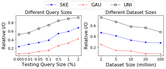
Figure 4. Performance of RL $\mathsf{ChooseSubtree}$

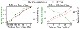
Figure 5. RL $\mathsf{ChooseSubtree}$ Query Processing Time

4.2.2. RL Split.

To evaluate the effect of RL $\mathsf{Split}$ on query performance, Figure 6 report results on the 3 synthetic datasets of different sizes by running range queries of different sizes. RL $\mathsf{Split}$ outperforms the R-Tree consistently over different query sizes, and the improvement can be up to 80%. We also observe that the RL $\mathsf{Split}$ model has better improvement on the R-Tree as the query size decreases. Possible reasons would be similar as we discussed in Section 4.2.1 for RL $\mathsf{ChooseSubtree}$.

The RL $\mathsf{Split}$ model also outperforms the R-Tree consistently over datasets of different sizes. Note that RL $\mathsf{Split}$ is trained on a small training dataset with only 100,000 data objects, but can be applied on large datasets successfully. Moreover, we also observe that as dataset size increases from 1 to 20 million, the improvement over the R-Tree generally increases on all 3 distributions. However, model performance slightly deteriorates as dataset size increases from 20 million to 100 million. The reason might be due to the inherent complicatedness of $\mathsf{Split}$. Node splitting results in the creation of 2 new nodes. As dataset size increases, the increase in tree height further contributes to this complicatedness because more nodes may be split from one $\mathsf{Split}$ process, and the RL $\mathsf{Split}$ model trained on 100,000 data objects would have more room for improvement.

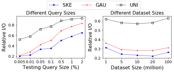
Figure 6. Performance of RL $\mathsf{Split}$

4.2.3. RLR-Tree.

This set of experiments is to evaluate the performance of RLR-Tree, which is constructed from a combined RL $\mathsf{ChooseSubtree}$ and RL $\mathsf{Split}$ model.

The Enhanced Training Process. We first compare the performance of RL $\mathsf{ChooseSubtree}$, RL $\mathsf{Split}$, Naive RLR-Tree, which is obtained by directly applying RL $\mathsf{ChooseSubtree}$ and RL $\mathsf{Split}$, and RLR-Tree, which uses the enhanced training process (Section 3.4), on all the 5 datasets in terms of relative I/O cost. As shown in Table 3, by applying the enhanced training process, RLR-Tree has the best performance on all datasets.

Table 3. RL $\mathsf{ChooseSubtree}$, RL $\mathsf{Split}$ and RLR-Tree

	SKE	GAU	UNI	CHI	IND
RLR-Tree	0.21	0.06	0.54	0.56	0.65
Naive RLR-Tree	0.24	0.08	0.58	0.61	0.67
RL $\mathsf{ChooseSubtree}$	0.29	0.08	0.56	0.60	0.67
RL $\mathsf{Split}$	0.22	0.28	0.58	0.63	0.71

Range queries. We evaluate the query performance of the RLR-Tree on all the 5 datasets using range queries of different sizes. Experimental results are shown in Figure 7. We observe that RLR-Tree outperforms the three baselines, the R-Tree, the R*-Tree, and the RR*-Tree, on all the synthetic datasets. The best performance is observed on the GAU dataset where RLR-Tree outperforms RR*-Tree by 78.6% and R*-Tree by 92% for query size 0.005%. On the other hand, on the 2 real datasets, RLR-Tree outperforms R*-Tree, RR*-Tree and LISA by up to 27.3%, 22.9% and 40% respectively. On all the 5 datasets, RLR-Tree has more significant advantages over baselines for smaller query sizes. This observation is consistent with RL $\mathsf{ChooseSubtree}$ and RL $\mathsf{Split}$ and possible reasons have been discussed in section 4.2.1. For query size 2% all the indices have similar performance, which is similar to the results reported in previous work (Qi et al., 2018).

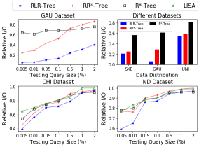
Figure 7. RLR-Tree Performance (Range Queries)

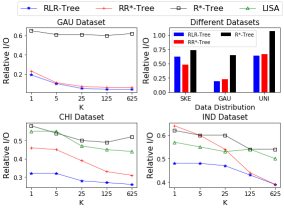
Figure 8. RLR-Tree Performance (KNN Queries)

KNN queries. To evaluate the performance of the RLR-Tree for types of queries that are not used in the model training process, we look into the K-Nearest-Neighbor (KNN) queries, which is a type of very popular spatial queries. A KNN query returns the $K$ nearest objects to a given query point. In our experiments, we consider different $K$ values, i.e. $K\in\{1,5,25,125,625\}$ with $K=1$ being the default. For each $K$ value, 1,000 uniformly distributed query points are randomly generated in the data space. We use the algorithms proposed in (Roussopoulos et al., 1995) to compute KNN queries accurately. In Figure 8, we observe that the RLR-Tree outperforms R*-Tree, RR*-Tree and LISA by up to 93.5%, 30.4% and 42% respectively. The RLR-Tree outperforms all the baselines in almost all the cases except for the SKE dataset. We also observe that the relative query performance of RLR-Tree to R-Tree gets better for larger $K$ values. The finding that the RLR-Tree also outperforms the baselines is particularly interesting —— the RLR-Tree is designed and trained to optimize the performance of range queries, rather than KNN queries. Additionally, we compute the reward and design the state features for the RLR-Tree in a way such that the model is trained to minimize the number of nodes accesses when answering range queries and not KNN queries. However, despite those design features that do not favour KNN queries, RLR-Tree still has the best performance most of the time for KNN queries.

4.2.4. Effect of Data Change

We run a series of experiments to evaluate the robustness of the RLR-Tree when changes in data distribution are encountered in dynamic environments.

Apply Trained Models on Different Data Distributions. In this set of experiments, we train RL $\mathsf{ChooseSubtree}$ and RL $\mathsf{Split}$ models on one dataset and apply the trained models to build RLR-Tree on a different dataset. Figure 9 reports relative I/O cost of the evaluated methods. For example, in Figure 9(a), we use the models trained on CHI and IND, respectively, to build different RLR-Trees on IND. On CHI and IND, we observe that though the models are trained on a different dataset, the constructed RLR-Trees still outperform all baselines for all query sizes except 2%. Note that compared with the RLR-Trees that are constructed by models trained on the same dataset, these RLR-Trees only experience a small degree of performance deterioration. This is perhaps because these real datasets share common features as they mostly consist of ”clusters” of high data density which represent developed regions surrounded by vast regions of low data density which represent rural areas. In contrast, for synthetic datasets, we use the models trained on the SKE dataset to build RLR-Trees for the GAU dataset and the UNI dataset. We observe that the performance deterioration of the RLR-Trees constructed with models trained on a different dataset is more significant. On GAU, although the RLR-Tree with SKE training is able to outperform all baselines for all query sizes, its query performance is up to 57% poorer than the RLR-Tree with GAU training. On UNI, we observe that the performance of RLR-Tree with SKE training is generally close to that of the RR*-Tree.

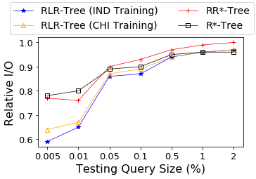
(a) IND Dataset

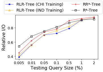
(b) CHI Dataset

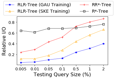
(c) GAU Dataset

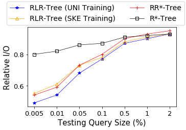
(d) UNI Dataset

Figure 9. Apply Trained Models on Other Data Distributions

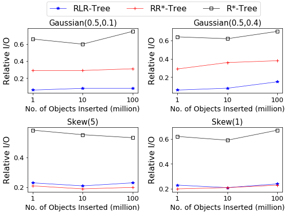
Figure 10. Updates with Different Data Distributions

Dynamic Updates with Gradual Data Change. This experiment is to investigate how well the RLR-Tree handles dynamic updates with gradual change of data distribution. Specifically, we first train and build 2 RLR-Trees of size 1 million using the GAU dataset with ($\mu=0.5$, $\sigma=0.2$) and the SKE dataset with ($c=9$) with their default settings respectively. For the RLR-Tree built using the GAU dataset, we insert up to 100 million spatial objects from GAU distribution with $(\mu=0.5$, $\sigma=0.1)$ and $(\mu=0.5$, $\sigma=0.4)$, and report the average relative I/O cost of 1,000 random queries, respectively. For the RLR-Tree built using the SKE dataset, we insert up to 100 million spatial objects from SKE distribution with $(c=5)$ and $(c=1)$, and report the average relative I/O cost of 1,000 random queries, respectively. Relevant experimental results are shown in Figure 10. We observe that despite inserting up to 100 times as many data objects from a different data distribution, RLR-Tree generally does not experience obvious performance deterioration. For the GAU dataset, RLR-Tree consistently outperforms all baselines. On the other hand, for the SKE dataset, RLR-Tree outperforms R*-Tree significantly but is slightly outperformed by RR*-Tree.

4.2.5. The Effects of Parameters

Training Dataset Size. This experiment is to evaluate the effect of training dataset size on the performance of the RLR-Tree. We would expect better query performance if we train the RL $\mathsf{ChooseSubtree}$ and RL $\mathsf{Split}$ models on the full dataset. However, the training is slow on large datasets. Instead, we propose to use a small training dataset. Experimental results are shown in Figure 11. First, we observe that the training time of RL $\mathsf{ChooseSubtree}$ model for different data distributions is similar, and increases significantly with the size of the training dataset. As expected, the query performance of the trained models improves as training dataset size increases from 25,000 to 100,000. However, the query performance becomes stable after the dataset size reaches 100,000, and the improvement of using training dataset of size 200,000 over 100,000 is not significant. The results for RL Split are qualitatively similar to those for RL $\mathsf{ChooseSubtree}$. Therefore we set training dataset size to be 100,000 by default which achieves a good tradeoff between training time and query performance. Note that RLR-Tree only needs to be trained once on a small training dataset and the learned models can be used on large dataset to build index and then to handle updates.

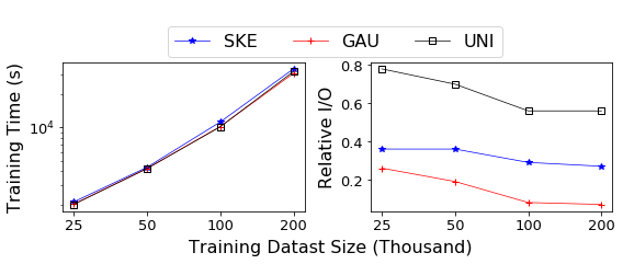
Figure 11. Effect of Varying Training Dataset Sizes

The Value of $k$. As shown in Figure 12(a), as top $k$ candidates are shortlisted to form the action space, the value of $k$ has a direct impact on the query performance of the resulted RLR-Tree. On one hand, when $k$ is larger, more actions are available to be selected for the trained model. On the other hand, model performance can be adversely affected when the action space is large as the trained model may not do a good job to filter out ”bad” candidates. To find a good $k$ value, we test different values of $k$ on the 3 synthetic datasets of size 500,000.

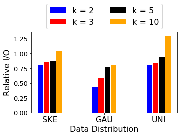
(a) Varying $k$ Values

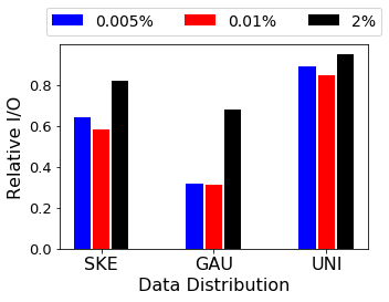
(b) Varying Training Query Sizes

Figure 12. The Effects of Parameters

We use RL $\mathsf{ChooseSubtree}$ as an example to show the effect of $k$. We observe qualitatively similar trends on all the 3 synthetic datasets. We make 2 observations. Firstly, recall that $k=1$ is the trivial case that generates the reference tree. By including one additional candidate in the action space, i.e., when $k=2$, we achieve significant query performance improvement for RL $\mathsf{ChooseSubtree}$. The best performance improvement is $56\%$ on the GAU dataset. Secondly, we observe that RL $\mathsf{ChooseSubtree}$ has the best result at $k=2$ for all the 3 datasets. As $k$ value increases, model performance deteriorates gradually. This observation aligns with our expectation. When $k$ value approaches and exceeds 10, the RL $\mathsf{ChooseSubtree}$ model starts to fail to outperform the R-Tree. We observe similar trends for RL $\mathsf{Split}$ on the 3 datasets, and do not report the result here due to space limitation.

Training Query Size. This experiment is to evaluate the effect of the training query size on the query performance of the resulted RLR-Tree. Figure 12(b) reports the average query performance of RL $\mathsf{ChooseSubtree}$ for each training query size for each dataset. We observe that the query performance of RL $\mathsf{ChooseSubtree}$ is rather poor when using the largest training query size, i.e. 2%. On the GAU dataset, the model performance with training query size of 2% is more than 100% poorer than that with our default setting of 0.01%. On the other hand, when using training query size of 0.005%, model performance is on par with our default setting on GAU dataset and shows slightly poorer results on SKE and UNI datasets. Therefore, we set the training query size to be 0.01% by default. We observe similar trends for RL $\mathsf{Split}$.

4.2.6. Other Experiments

Number of Dimensions. This experiment is to show how well RLR-Tree scales with dimensions. We vary the number of dimensions from 2 to 10. For each case, we generate a synthetic dataset with 20 million objects following the Uniform distribution. The Uniform distribution is chosen because it is commonly used for high dimension synthetic datasets in previous works (Beckmann and Seeger, 2009; Nathan et al., 2020). For each dataset, we report the average relative I/O cost for answering 1,000 random queries for each index in Figure 14. The average data selectivity of the query workload for each dataset is kept constant at 0.01%. We observe that RLR-Tree consistently outperforms all baselines all the time. Moreover, its advantage becomes more significant as the number of dimensions increases, which illustrates the robustness of RLR-Tree w.r.t. the number of dimensions.

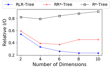
Figure 13. Changing Dimensions

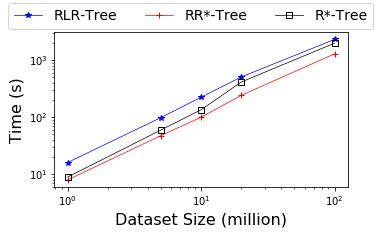
Figure 14. Index construction time

Index Construction Time and Size. The index construction time is similar for different data distributions of the same size, and we use the GAU dataset as an example. As shown in Figure 14, index construction time increases almost linearly with increase in dataset size. Note that the construction time of RLR-Tree is comparable to that of R*-Tree and RR*-Tree. And we expect RLR-Tree construction time to be shorter when using better GPU devices. For index size, the RLR-Tree and other baselines almost have the same size. Therefore, we report the RLR-Tree sizes for datasets of different sizes. As shown in Table 4, RLR-Tree size increases linearly as dataset size increases.

Table 4. Index size for GAU datasets

Dataset size (million)	1	5	10	20	100
RLR-Tree size (MB)	39	195	390	780	3900

5. Related Work

5.1. Spatial Indices

We next introduce three categories of spatial indices.

Data partitioning based indices: R-Tree and its variants. The category of indices partitions the dataset into subsets and indexes the subsets. Typical examples include the R-Tree and its variants, such as R^∗-Tree (Beckmann et al., 1990), R⁺-Tree (Sellis et al., 1987), RR^∗-Tree (Beckmann and Seeger, 2009). An R-Tree is usually built through a one-by-one insertion approach, and is maintained by dynamic updates. As discussed in Section 1, these R-Tree variants are equipped with various heuristic rules for the two key operations of building an R-Tree, $\mathsf{ChooseSubtree}$ or $\mathsf{Split}$, but none of the rules have dominant query performance. This partly motivates us to design learning-based solutions for $\mathsf{ChooseSubtree}$ and $\mathsf{Split}$ operations in this work.

There exist R-Tree variants that explore the query workload property or the special property of data. For example, in QUASII (Pavlovic et al., 2018) and CUR-Tree (Ross et al., 2001), the query workload is utilized to build an R-Tree. These extensions are orthogonal to our work.

Data partitioning based indices: Packing. An alternative way of building an R-Tree is to pack data points into leaf nodes and then build an R-Tree bottom up. The original R-Tree and almost all of its variants are designed for a dynamic environment, being able to handle insertions and deletions, while packing methods are for static databases (Kamel and Faloutsos, 1993). Packing needs to have all the data before building indices, which are not always available in many situations. The existing packing methods explore different ways of sorting spatial objects to achieve better ordering of the objects and eventually better packing. Some ordering methods (Arge et al., 2008) are based on the coordinates of objects, such as STR (Leutenegger et al., 1997), TGS (García R et al., 1998) and the lowx packed R-Tree (Roussopoulos and Leifker, 1985) and other ordering methods are based on space filling curves such as z-ordering (Orenstein, 1986; Qi et al., 2018), Gray coding (Faloutsos, 1986) and the Hilbert curve (Faloutsos and Roseman, 1989).

Other spatial indices. In space partitioning based indices, such as kd-Tree (Bentley, 1975) and Quad-Tree (Finkel and Bentley, 1974), the space is recursively partitioned until the number of objects in a partition reaches a threshold.

5.2. Learned Indices

Learned one-dimensional indices. The idea behind learned index is to learn a function that maps a search key to the storage address of a data object. The idea of learned indices is first introduced by (Kraska et al., 2018), which proposes the Recursive Model Index (RMI) to learn the data distribution in a hierarchical manner. It essentially learns a cumulative distribution function (CDF) using a neural network to predict the rank of a search key. The idea inspires a number of follow-up studies (Ding et al., 2020a; Ferragina and Vinciguerra, 2020; Kipf et al., 2020; Wu et al., 2021) on learned indices.

Learned spatial indices. Inspired by the idea of learned one-dimensional indices, several learned spatial indices have been proposed. The Z-order model (Wang et al., 2019) extends RMI to spatial data by using a space filling curve to order data points and then learning the CDF to map the key of a data point to its rank. Recursive spatial model index (RSMI) (Qi et al., 2020) further develops the Z-order idea (Wang et al., 2019) and RMI. RSMI maps the data points to a rank space using the rank space-based transformation technique (Qi et al., 2018). LISA (Li et al., 2020) is a disk-based learned index. It partitions the data space with a grid, numbers the grid cells, and learns a data distribution based on this numbering. Similar to Z-order model (Wang et al., 2019) and RSMI (Qi et al., 2020), Flood (Nathan et al., 2020) also maps a dataset to a uniform rank space before learning a CDF. Differently, it utilizes workload to optimize the learning of the CDF, and it learns the CDF of each dimension separately. Tsunami (Ding et al., 2020b) extends Flood to better utilize workload to overcome the limitation of Flood in handling skewed workload and correlated data. The ML-Index (Davitkova et al., 2020) generalizes the idea of the iDistance scaling method (Jagadish et al., 2005) to map point objects to a one-dimensional space and then learns the CDF.

Remark. These learned indices all aim to learn a CDF for a particular data to replace the traditional indices. However, RLR-Tree is fundamentally different —— Instead of learning any CDF, we train RL models to handle $\mathsf{ChooseSubtree}$ and $\mathsf{Split}$ operations. Furthermore, these learned indices have the following limitations compared with our solution: First, they can only handle spatial point objects while our proposed method is able to handle any spatial data, such as rectangular objects. Second, they all need customized algorithms to handle each type of query. They focus on certain types of queries and it is not clear how they can process other types of queries. For example, some of them  (Nathan et al., 2020; Ding et al., 2020b; Davitkova et al., 2020) do not consider KNN queries, an important type of spatial queries; Some learned indices (Li et al., 2020) extend their algorithm for range queries to handle KNN queries by issuing a series of range queries until $k$ points are found. However, the query performance largely depends on the size of the region used. In contrast, the RLR-Tree simply uses existing query processing algorithms for R-Tree to handle different types of queries. Third, some of these learned indices (Wang et al., 2019; Qi et al., 2020) return approximate query results while our query results are accurate. Fourth, both Flood and Tsunami need the query workload as the input. However, we do not assume the query workload to be known. Finally, updates are not discussed for Flood, Tsunami or the ML-Index. Although RSMI (Qi et al., 2020) and LISA (Li et al., 2020) can handle updates, their models have to be retrained periodically to retain good query performances. In contrast, our proposed RLR-Tree readily handles updates without the need to keep retraining the models.

5.3. Applications of Reinforcement Learning

To the best of our knowledge, no work is done to use RL to improve on the R-Tree index or its variants. RL has been successfully applied to solve other database applications, such as database tuning tasks (Trummer et al., 2019; Zhang et al., 2019; Liang et al., 2019a), similarity search (Wang et al., 2020), join order selection (Yu et al., 2020), index selection (Sadri et al., 2020), and QD-Tree for data partitioning (Yang et al., 2020). In particular, to build a QD-Tree, an RL model is trained to learn a policy to make partitioning decisions to maximize the data skipping ratio for a given query workload. The MDP design of our RLR-Tree is fundamentally different from that of QD-Tree, which is based on NeuroCuts (Liang et al., 2019b), in at least three aspects. 1) State design: QD-Tree follows a tree-structured MDP where a cut at a node (state) creates 2 new nodes (next states). In contrast, in an RLR-Tree, an RL ChooseSubtree decision at a node (state) leads to the selected child node (next state) and an RL Split decision at a node (state) leads to the parent node (next state). 2) Action space: For QD-Tree, the query workload is assumed to be known and candidate cuts are generated from a standard SQL planner. For RLR-Tree, we do not assume any prior knowledge of the query workload and have to come out with suitable actions ourselves. 3) Reward: Among others, QD-Tree computes rewards after the whole tree is built, while RLR-Tree computes rewards after each splitting/insertion process. We would also like to highlight that QD-Tree cannot handle updates as the RLR-Tree does.

6. Conclusions and Future Work

We propose the RLR-Tree to improve on the R-Tree and its variants designed for a dynamic environment. Experimental results show that RLR-Tree is able to outperform the RR*-Tree, the best R-Tree variant, by up to 78.6% for range queries and up to 30.4% for KNN queries. Although the models of the RLR-Tree are trained on a small training dataset of size 100,000, the trained models are readily applied on large datasets and are able to handle dynamic updates even with changes in data distribution.

This work take a first step to use machine learning to improve on the R-Tree, and we believe it we would open a few promising directions for future work: 1) further explore and refine the designs of the states, the action space and the reward signal; 2) extend the idea to index enriched spatial data, such as spatial-temporal data, moving objects, and spatial-textual data; 3) explore other machine learning models.

References

- (1)
- Arge et al. (2008) Lars Arge, Mark De Berg, Herman Haverkort, and Ke Yi. 2008. The priority R-tree: A practically efficient and worst-case optimal R-tree. ACM Transactions on Algorithms (TALG) 4, 1 (2008), 1–30.
- Beckmann et al. (1990) Norbert Beckmann, Hans-Peter Kriegel, Ralf Schneider, and Bernhard Seeger. 1990. The R*-tree: an efficient and robust access method for points and rectangles. In Proceedings of the 1990 ACM SIGMOD international conference on Management of data. 322–331.
- Beckmann and Seeger (2009) Norbert Beckmann and Bernhard Seeger. 2009. A revised r*-tree in comparison with related index structures. In Proceedings of the 2009 ACM SIGMOD International Conference on Management of data. 799–812.
- Bentley (1975) Jon Louis Bentley. 1975. Multidimensional binary search trees used for associative searching. Commun. ACM 18, 9 (1975), 509–517.
- Davitkova et al. (2020) Angjela Davitkova, Evica Milchevski, and Sebastian Michel. 2020. The ML-Index: A Multidimensional, Learned Index for Point, Range, and Nearest-Neighbor Queries.. In EDBT. 407–410.
- Ding et al. (2020a) Jialin Ding, Umar Farooq Minhas, Jia Yu, Chi Wang, Jaeyoung Do, Yinan Li, Hantian Zhang, Badrish Chandramouli, Johannes Gehrke, Donald Kossmann, et al. 2020a. ALEX: an updatable adaptive learned index. In Proceedings of the 2020 ACM SIGMOD International Conference on Management of Data. 969–984.
- Ding et al. (2020b) Jialin Ding, Vikram Nathan, Mohammad Alizadeh, and Tim Kraska. 2020b. Tsunami: A learned multi-dimensional index for correlated data and skewed workloads. arXiv preprint arXiv:2006.13282 (2020).
- Faloutsos (1986) Christos Faloutsos. 1986. Multiattribute hashing using gray codes. In Proceedings of the 1986 ACM SIGMOD international conference on Management of data. 227–238.
- Faloutsos and Roseman (1989) Christos Faloutsos and Shari Roseman. 1989. Fractals for secondary key retrieval. In Proceedings of the eighth ACM SIGACT-SIGMOD-SIGART symposium on Principles of database systems. 247–252.
- Ferragina and Vinciguerra (2020) Paolo Ferragina and Giorgio Vinciguerra. 2020. The PGM-index: a fully-dynamic compressed learned index with provable worst-case bounds. Proceedings of the VLDB Endowment 13, 10 (2020), 1162–1175.
- Finkel and Bentley (1974) Raphael A. Finkel and Jon Louis Bentley. 1974. Quad trees a data structure for retrieval on composite keys. Acta informatica 4, 1 (1974), 1–9.
- García R et al. (1998) Yván J García R, Mario A López, and Scott T Leutenegger. 1998. A greedy algorithm for bulk loading R-trees. In Proceedings of the 6th ACM international symposium on Advances in geographic information systems. 163–164.
- Greene (1989) Diane Greene. 1989. An implementation and performance analysis of spatial data access methods. In Proceedings. Fifth International Conference on Data Engineering. IEEE Computer Society, 606–607.
- Guttman (1984) Antonin Guttman. 1984. R-trees: A dynamic index structure for spatial searching. In Proceedings of the 1984 ACM SIGMOD international conference on Management of data. 47–57.
- Jagadish et al. (2005) Hosagrahar V Jagadish, Beng Chin Ooi, Kian-Lee Tan, Cui Yu, and Rui Zhang. 2005. iDistance: An adaptive B+-tree based indexing method for nearest neighbor search. ACM Transactions on Database Systems (TODS) 30, 2 (2005), 364–397.
- Kamel and Faloutsos (1993) Ibrahim Kamel and Christos Faloutsos. 1993. On packing R-trees. In Proceedings of the second international conference on Information and knowledge management. 490–499.
- Kanth et al. (1997) Kothuri Venkata Ravi Kanth, Divyakant Agrawal, Ambuj K Singh, and Amr El Abbadi. 1997. Indexing non-uniform spatial data. In Proceedings of the 1997 International Database Engineering and Applications Symposium (Cat. No. 97TB100166). IEEE, 289–298.
- Kipf et al. (2020) Andreas Kipf, Ryan Marcus, Alexander van Renen, Mihail Stoian, Alfons Kemper, Tim Kraska, and Thomas Neumann. 2020. RadixSpline: a single-pass learned index. In Proceedings of the Third International Workshop on Exploiting Artificial Intelligence Techniques for Data Management. 1–5.
- Klambauer et al. (2017) Günter Klambauer, Thomas Unterthiner, Andreas Mayr, and Sepp Hochreiter. 2017. Self-normalizing neural networks. Advances in neural information processing systems 30 (2017), 971–980.
- Kraska et al. (2018) Tim Kraska, Alex Beutel, Ed H Chi, Jeffrey Dean, and Neoklis Polyzotis. 2018. The case for learned index structures. In Proceedings of the 2018 International Conference on Management of Data. 489–504.
- Leutenegger et al. (1997) Scott T Leutenegger, Mario A Lopez, and Jeffrey Edgington. 1997. STR: A simple and efficient algorithm for R-tree packing. In Proceedings 13th International Conference on Data Engineering. IEEE, 497–506.
- Li et al. (2020) Pengfei Li, Hua Lu, Qian Zheng, Long Yang, and Gang Pan. 2020. LISA: A learned index structure for spatial data. In Proceedings of the 2020 ACM SIGMOD International Conference on Management of Data. 2119–2133.
- Liang et al. (2019b) Eric Liang, Hang Zhu, Xin Jin, and Ion Stoica. 2019b. Neural packet classification. In Proceedings of the ACM Special Interest Group on Data Communication. 256–269.
- Liang et al. (2019a) Xi Liang, Aaron J Elmore, and Sanjay Krishnan. 2019a. Opportunistic view materialization with deep reinforcement learning. arXiv preprint arXiv:1903.01363 (2019).
- Mnih et al. (2015) Volodymyr Mnih, Koray Kavukcuoglu, David Silver, Andrei A Rusu, Joel Veness, Marc G Bellemare, Alex Graves, Martin Riedmiller, Andreas K Fidjeland, Georg Ostrovski, et al. 2015. Human-level control through deep reinforcement learning. Nature 518, 7540 (2015), 529–533.
- Nathan et al. (2020) Vikram Nathan, Jialin Ding, Mohammad Alizadeh, and Tim Kraska. 2020. Learning multi-dimensional indexes. In Proceedings of the 2020 ACM SIGMOD International Conference on Management of Data. 985–1000.
- Orenstein (1986) Jack A Orenstein. 1986. Spatial query processing in an object-oriented database system. In Proceedings of the 1986 ACM SIGMOD international conference on Management of data. 326–336.
- Pandey et al. (2020) Varun Pandey, Alexander van Renen, Andreas Kipf, Ibrahim Sabek, Jialin Ding, and Alfons Kemper. 2020. The case for learned spatial indexes. arXiv preprint arXiv:2008.10349 (2020).
- Pavlovic et al. (2018) Mirjana Pavlovic, Darius Sidlauskas, Thomas Heinis, and Anastasia Ailamaki. 2018. QUASII: query-aware spatial incremental index. In 21st International Conference on Extending Database Technology (EDBT).
- Puterman (2014) Martin L Puterman. 2014. Markov decision processes: discrete stochastic dynamic programming. John Wiley & Sons.
- Qi et al. (2020) Jianzhong Qi, Guanli Liu, Christian S Jensen, and Lars Kulik. 2020. Effectively learning spatial indices. Proceedings of the VLDB Endowment 13, 12 (2020), 2341–2354.
- Qi et al. (2018) Jianzhong Qi, Yufei Tao, Yanchuan Chang, and Rui Zhang. 2018. Theoretically optimal and empirically efficient r-trees with strong parallelizability. Proceedings of the VLDB Endowment 11, 5 (2018), 621–634.
- Ross et al. (2001) Kenneth A Ross, Inga Sitzmann, and Peter J Stuckey. 2001. Cost-based unbalanced R-trees. In Proceedings Thirteenth International Conference on Scientific and Statistical Database Management. SSDBM 2001. IEEE, 203–212.
- Roussopoulos et al. (1995) Nick Roussopoulos, Stephen Kelley, and Frédéric Vincent. 1995. Nearest neighbor queries. In Proceedings of the 1995 ACM SIGMOD international conference on Management of data. 71–79.
- Roussopoulos and Leifker (1985) Nick Roussopoulos and Daniel Leifker. 1985. Direct spatial search on pictorial databases using packed R-trees. In Proceedings of the 1985 ACM SIGMOD international conference on Management of data. 17–31.
- Sadri et al. (2020) Zahra Sadri, Le Gruenwald, and Eleazar Leal. 2020. Online index selection using deep reinforcement learning for a cluster database. In 2020 IEEE 36th International Conference on Data Engineering Workshops (ICDEW). IEEE, 158–161.
- Sellis et al. (1987) Timos Sellis, Nick Roussopoulos, and Christos Faloutsos. 1987. The R+-Tree: A Dynamic Index for Multi-Dimensional Objects. Technical Report.
- Trummer et al. (2019) Immanuel Trummer, Junxiong Wang, Deepak Maram, Samuel Moseley, Saehan Jo, and Joseph Antonakakis. 2019. Skinnerdb: Regret-bounded query evaluation via reinforcement learning. In Proceedings of the 2019 International Conference on Management of Data. 1153–1170.
- Wang et al. (2019) Haixin Wang, Xiaoyi Fu, Jianliang Xu, and Hua Lu. 2019. Learned Index for Spatial Queries. In 2019 20th IEEE International Conference on Mobile Data Management (MDM). IEEE, 569–574.
- Wang et al. (2020) Zheng Wang, Cheng Long, Gao Cong, and Yiding Liu. 2020. Efficient and effective similar subtrajectory search with deep reinforcement learning. Proceedings of the VLDB Endowment 13, 12 (2020), 2312–2325.
- Wu et al. (2021) Jiacheng Wu, Yong Zhang, Shimin Chen, Jin Wang, Yu Chen, and Chunxiao Xing. 2021. Updatable Learned Index with Precise Positions. arXiv preprint arXiv:2104.05520 (2021).
- Yang et al. (2020) Zongheng Yang, Badrish Chandramouli, Chi Wang, Johannes Gehrke, Yinan Li, Umar Farooq Minhas, Per-Åke Larson, Donald Kossmann, and Rajeev Acharya. 2020. Qd-tree: Learning data layouts for big data analytics. In Proceedings of the 2020 ACM SIGMOD International Conference on Management of Data. 193–208.
- Yu et al. (2020) Xiang Yu, Guoliang Li, Chengliang Chai, and Nan Tang. 2020. Reinforcement learning with tree-lstm for join order selection. In 2020 IEEE 36th International Conference on Data Engineering (ICDE). IEEE, 1297–1308.
- Zhang et al. (2019) Ji Zhang, Yu Liu, Ke Zhou, Guoliang Li, Zhili Xiao, Bin Cheng, Jiashu Xing, Yangtao Wang, Tianheng Cheng, Li Liu, et al. 2019. An end-to-end automatic cloud database tuning system using deep reinforcement learning. In Proceedings of the 2019 International Conference on Management of Data. 415–432.