Weather Analogs with a Machine Learning Similarity Metric for
Renewable Resource Forecasting

Abstract

The Analog Ensemble (AnEn) technique is a technique that has been shown effective on several weather problems. Unlike previous weather analogs that are sought within a large spatial domain and an extended temporal window, AnEn strictly confines space and time, and independently generates results at each grid point within a short time window. AnEn can find similar forecasts that lead to accurate and calibrated ensemble forecasts.

The central core of the AnEn technique is a similarity metric that sorts historical forecasts with respect to a new target prediction. A commonly used metric is a Euclidean distance function which computes the distance between a target and a historical set of forecasts using a weighted difference of all multivariate parameters, normalized by the standard deviation of the historical set. A significant difficulty using this metric is the definition of the weights for all the parameters. Generally, the AnEn methodology starts with a feature selection task, where a subset of parameters are selected, and then weights are identified using heuristics or an optimization process. While this method has been proven effective, it is expedient and error inducing. AnEn is, in fact, characterized by a systematic bias when applied to extreme events, and this bias can potentially be hard to compensate if only a limited set of historical forecasts is available.

This paper proposes a novel definition of weather analogs through a Machine Learning (ML) based similarity metric. The similarity metric uses neural networks that are trained and instantiated to search for weather analogs. This new metric allows incorporating all variables without requiring a prior feature selection and weight optimization. Experiments are presented on the application of this new metric to forecast wind speed and solar irradiance. Results show that the ML metric generally outperforms the original metric. The ML metric has a better capability to correct for larger errors and to take advantage of a larger search repository. Spatial predictions using a learned metric also show the ability to define effective latent features that are transferable to other locations.

1 Introduction

Analog Ensemble (AnEn) [1] is a technique to generate ensemble predictions from a deterministic Numerical Weather Prediction (NWP) model and the corresponding observations. Different from its predecessors [2, 3], AnEn identifies weather analogs independently at each grid point [4] over a short time window, e.g., three hours, which is sometimes referred to as the Independent Search (IS) AnEn [5]. AnEn works seamlessly with high-resolution NWP models because predictions at each model grid can be directly input into AnEn to generate prediction ensembles. IS allows AnEn to be computationally efficient when deployed to supercomputers [6, 7].

AnEn has been shown to generate accurate and calibrated ensembles in forecasting renewable energy resources, e.g., solar irradiance and wind speed. To generate final power forecasts, these meteorological forecasts can be coupled with an additional energy simulator or can be used with the actual observed power data during the analog ensemble generation to predict power. Alessandrini et al. applied AnEn to short-term Photovoltaic (PV) power forecasts at three power plants at Italy. They compared AnEn with a quantile regression method and a persistence model and showed that AnEn were better calibrated and had a lower error. Cervone et al. investigated the performance of AnEn plus a feed-forward neural network to further account for the physical and the engineering bias. Both Missing Rate Error (MRE) and Continuous Rank Probability Score (CRPS) were improved, showing better forecast accuracy and ensemble quality. Zhang et al. proposed a blending technique that combines weather analogs from multiple NWP models for day-ahead PV energy market forecast. Experiments were carried out for Southeastern Massachusetts and showed that the blending technique reduces about 60% of the error compared to a persistence model and around 20% compared to baseline NWP models and a data-driven Support Vector Machine (SVM) model. Wang et al. extended the work of Zhang et al. to the forecasting of PV power ramps and frequent fluctuations in energy production within the next hour. They proposed to use meteorological forecasts from a persistence model because it has a high accuracy for very short-term forecasts and avoids the computational complexity involved with running NWP models. Results showed that it outperformed six baseline models, reaching up to a 40% of error reduction. The capability of AnEn generating accurate and calibrated ensembles has also been studied and tested for wind speed forecast at the surface [8], in the stratosphere [11], and air quality predictions [12]. Vanvyve et al. and Shahriari et al. applied AnEn for long-term and large-scale wind energy assessment. Results showed that the uncertainty information reconstructed by AnEn is more accurate and more reliable compared to other statistical and dynamical ensembles.

AnEn, as it was originally defined, defines a weather similarity metric, shown in Equation (1). The fact that weather analogs are sought with a short temporal window at each location drastically reduces the degrees of freedom of the problem at stake. Given an adequate forecast model, AnEn is able to find similar historical forecasts and then uses the corresponding observations to correct for forecast biases that might be present in the current model forecast. There are some key aspects of the current metric definition: (1) prior knowledge on predictors and the associated weights are needed for optimal performance. AnEn benefits from using a few predictors to identify weather analogs and it is sensitive to predictor weights [15]. Since weight optimization is a computationally expansive procedure, typically AnEn is run using only a few predictors, although NWP models simulate hundreds. (2) AnEn assumed a frozen model. In an operational environment, however, NWP models are constantly subject to parameter changes. These parameterization updates are intended for better performance of the NWP model, but they might break the assumption of a static model and, as a result, AnEn might not yield the expected improvement when a longer search period (e.g., spanning several years) is used.

The paper seeks to address the above issues by proposing an Machine Learning (ML) based similarity metric, inspired by the recent progress in target detecting and face recognition in Computer Vision (CV). Face recognition systems are able to associate a face with an identity. The key idea is that, instead of matching two face images on a pixel basis, high-level features from face images are first extracted, such as eyes and noses. These features are then compared against all the features present in a database. If a satisfactory match can be found, the associated identification in the database is queried and used as the output of the system. Presumably, there are thousands of features one can define to describe a person’s face, e.g., the skin color, the curvature of eyebrows, and the shape of the nose. However, the features used by an ML algorithm are optimized to separate images of different identities and cluster images of the same identity. These features are usually learnable, and the approach to building effective facial features is model training. A more in-depth review on this matter is provided in Section 2.2.

Neural Network (NN) has been used for power forecasting [16, 17, 18, 19]. In this work, we extend the original AnEn by using a non-linear similarity metric driven by a deep embedding network, namely an Long Short-Term Memory (LSTM) network structure. Instead of using NN as an end-to-end modeling technique as in the contributions mentioned above for power, here we seek to refine the AnEn forecast generation with a more powerful metric characterized by a group of trained equations rather than a single equation to account for the high level of complexity in NWP models. Building effective weather features requires model training and therefore, model training requires known similar and dissimilar weather patterns as targets. We propose a reverse analog technique to automatically select forecast pairs that could be used during the model training.

The rest of the paper is organized as follows: Section 2 introduces, in order, the original AnEn, the proposed architecture with NN, and then the reverse analogs as an effective auto-labeling technique during model training; Section 3 describes the observational and NWP forecast data used in this research; Section 4 shows results of the various aspects in ensemble verification; finally, Section 5 includes a summary and conclusions.

2 Methodology

2.1 Analog Ensemble

AnEn generates forecast ensembles from an archive of deterministic model predictions and the corresponding observations of interest. AnEn first identifies the $M$ most similar historical forecasts to the current target forecast and then, the observations corresponding to the selected historical forecasts consist of the ensemble members. This process is repeated for each forecast cycle time (e.g., when the forecast was initiated), each forecast lead time, and each grid location independently. The parameter $M$, also called the number of analog ensemble members, is usually an integer number larger than five. The choice is often practical and depends on the size of the historical archive of predictions and observations.

AnEn can generate accurate and representative forecast ensembles from a deterministic forecast model. It assumes that similar weather forecasts have similar error patterns and these errors can be corrected when using observations associated with similar weather forecasts. The end forecast product, being an ensemble of historical observations, is able to compensate for the random bias, possibly associated with the observations and the underlying forecasts.

The key component of AnEn is the definition of weather similarity. Delle Monache et al. proposed the following equation as a measure for dissimilarity:

$$\|F_{t},A_{t^{\prime}}\|=\sum_{i=1}^{N_{v}}\frac{w_{i}}{\sigma_{f_{i}}}\sqrt{\sum_{j=-\tilde{t}}^{\tilde{t}}(F_{i,t+j}-A_{i,t^{\prime}+j})^{2}},$$ (1)

where $F_{t}$ is the multivariate target forecast at the time $t$; $A_{t^{\prime}}$ is a historical multivariate analog forecast at a historical time point $t^{\prime}$; $N_{v}$ is the number of variables from forecasts; $w_{i}$ is the weight parameter for the forecast variable $i$ as its importance; $\sigma_{f_{i}}$ is the standard deviation of the respective variable during the historical time period; $\tilde{t}$ indicates a short time window over which the metric is computed and it equals half the number of the additional time points to consider; finally, $F_{i,t+j}$ and $A_{i,t^{\prime}+j}$ are are the values of the respective target forecast and the past analog forecast in the time window for the variable $i$.

This metric has been proven to work in various circumstances [15, 20, 1, 21, 22, 23]. Its efficient implementation [24] and application to large scale simulation [6] have also been studied with success. AnEn thrives in cases where historical archives of observations and forecasts are sufficient and the uncertainty information associated with a deterministic prediction is desired. It provides an accurate and computationally efficient solution to the statistical reconstruction of ensemble members.

The current definition of weather similarity, however, poses a dilemma in its optimization process. For example, most of the past literature has been involving only a handful of predictors to calculate the dissimilarity metric while, in reality, NWP models usually provide simulations for hundreds of weather variables that characterize a wide range of the vertical profile at a certain location. Although using fewer parameters can be more permissive to finding weather analogs with lower dissimilarity metric but these analogs might not actually be the “good analogs” [2, 3] in a physical sense. To another extreme, if all variables have been fed into the dissimilarity calculation in favor of finding better weather analogs in the physical sense, weight optimization then becomes a significant factor that impedes its successful application. The AnEn performance depends heavily on the parameter weights. Currently, sensitivity studies on identifying the best weight combination usually use an extensive search algorithm or a random sampling technique. The computation of the extensive search algorithm scales exponentially with the number of variables while the random sampling technique does not guarantee to give you the optimal solution. Neither these approaches are suitable for ingesting a large number of predictor variables. As a result, the process of finding weather analogs is usually confined within a few parameters, and it is subject to individual researchers to provide a good combination of weights to the best of their knowledge.

Another potential limitation is that, the current metric uses a linear combination of weather variables to formulate the similarity metric. It is, however, likely that the response variable has a non-linear relationship with the predictor variables. Part of the non-linearity can be approximated when using the actual observations as ensemble members. But the linear assumption for defining weather analogs can still cause problems in cases of rare events. AnEn forecasts have been found to have a systematic bias when predicting extreme events, e.g., extreme wind speed [25] and heatwaves [26, 27]. On the other hand, if the predictor variables per se are associated with a significant error, the weather analogs generated using these variables will also be compromised and they only contribute to a wrong type of ensembles. A potential solution is to consider a larger pool of predictor variables and formulate an overall non-linear similarity measure.

In the following sections, an Artificial Intelligence (AI) framework for identifying weather analogs combining a triplet structure and an LSTM network is proposed. Details of the framework and the training techniques are then introduced.

2.2 Machine Learning Model Architecture

Computer scientists have long sought algorithms for efficient feature transformation and learning. Throughout the years, NN have become increasingly popular and reliable for achieving impressive results on tasks like image classification and face recognition. Siamese and triplet NN s are specifically designed to solve problems of identifying similar images and produce representative embeddings. Baldi and Chauvin and Bromley et al. are probably the first groups to formulate the early ideas of the Siamese networks. The Siamese network is a type of NN for tackling image identification. Instead of training a network that generates a binary output, e.g., whether two images are similar or not, the Siamese network focuses the model training on generating effective embedding vectors. These embedding vectors, also referred to as the feature vectors, characterize the original image with fewer digits. For example, an RGB image with a dimension of 128x128x3 pixels can be compressed to an embedding vector containing only 16 values. The original image representation in pixels usually has redundant information, e.g., nearby pixels having similar colors. Thus, the embedding vector seeks a efficient and compact representation of the original image. This process is referred to as image compression or dimensionality reduction. The Siamese network is particularly effective at training embedding networks. Model weights are tuned so that similar images are placed closer to each other in a transformed space and dissimilar images are placed further away. Baldi and Chauvin proposed to use the Siamese network and this type of training technique to extract features from fingerprints. Bromley et al. developed a similar architecture independently to solve signature verification problems and coined the term Siamese network. More recent work has focused on the effectiveness of such a learned embedding. Chopra et al. proposed that Siamese networks should be trained in a competitive style to encourage smaller distances between similar targets and larger distances between dissimilar targets. Human-level performance in face recognition was achieved using such an architecture [31].

At this point, the Siamese network is able to handle two input images at a time, e.g., predicting whether two face images are of the same individual. It is, however, limited in cases where a new face image is provided and the goal is to predict whether it is of individual A or B. As a result, Siamese networks were soon extended to triplet networks. Three, rather than two, images are used during one iteration of training. The three input images are referred to as the anchor, the positive, and the negative images. The convention is that the anchor image is more similar to the positive image than to the negative image. They were designed to encourage more general and robust high-level embeddings than their predecessor because, during training, the network receives guidance not only on how two images are similar, but also how two images are different. Triplet networks have outperformed Siamese networks in generating embeddings with less contextual information [32]. Later research shown interest in both approaches, using the Siamese [33, 34, 35, 36] and the triplet [37, 38] networks for tasks like classification and tracking.

The key idea of a triplet network is the scheme that shares model parameters during model training. During forward propagation, three images are processed and compressed but this is not accomplished with three different models. Rather, the embeddings for input images are generated using the same embedding network. This is usually referred to, in the literature, as “copies” of the network but, in practice, these embedding networks have the same weight during training. This scheme contributes to two important properties [33]: prediction consistency and network symmetry. Prediction consistency ensures that similar inputs are mapped to a hyperspace with close vicinity and dissimilar inputs are mapped with large distances; network symmetry ensures that the order within input pairs (or triplets) will not affect the final prediction. This is important for building an effective transformation so that similar observations are indeed associated with similar weather forecasts.

This paper follows the paradigm of a triplet network. An LSTM network is used as the embedding network. Hochreiter and Schmidhuber proposed LSTM to encode sequence information of arbitrary lengths and it has been successfully applied to time series prediction tasks [40, 17, 18, 19, 41]. LSTM uses memory cells and gate units to allow information from previous time lags to flow easily into later predictions. Recall the term $\tilde{t}$ from Equation (1) indicating a time window. This parameter is usually set to 1 but it can vary based on the application. In other words, when generating AnEn, the length of time series could vary depending on the time window size. Therefore, the ability to encode an arbitrarily long time sequence is desired when generating embeddings for similarity calculation.

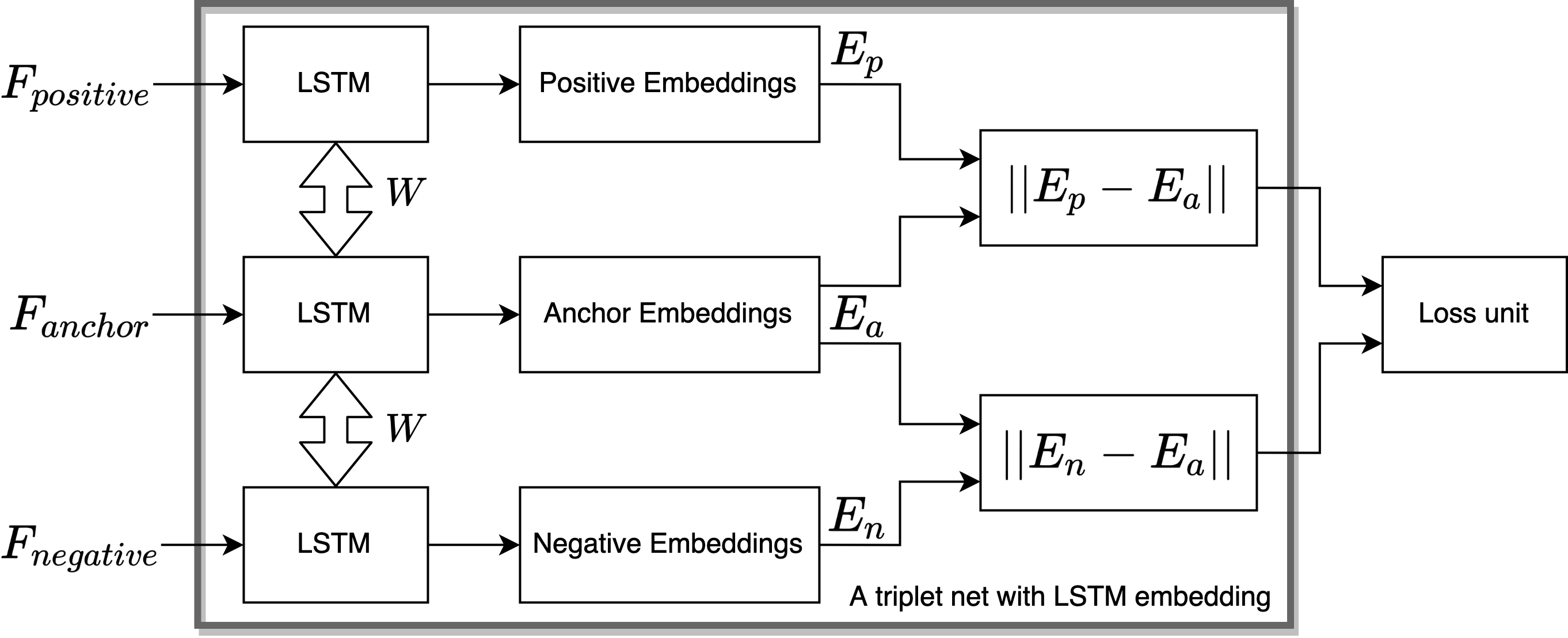
Figure 1: Triplet architecture with an LSTM embedding network. $F$ denotes the multivariate forecast time series; $E$ denotes the embeddings; $p$ denotes the positive case; $a$ denotes the anchor case; $n$ denotes the negative case.

Figure 1 shows the architecture proposed in this paper, and the mathematical formulation is as follows: we seek to find a transformation function group $E_{W}(F)$ parameterized by $W$ and acting on a multivariate forecast time series $F$ so that, given the observations having Euclidean distances $||O_{a}-O_{p}||<||O_{a}-O_{n}||$, the transformation function gives $||E_{W}(F_{a})-E_{W}(F_{p})||<||E_{W}(F_{a})-E_{W}(F_{n})||$, where $a$, $p$, and $n$ denote the anchor, positive, and negative cases. Note that in this work, $E_{W}(F)$, rather than being a single function, consists of a group of functions characterized by an LSTM network.

To explain in more details, the function group $E_{W}$ performs a non-linear feature transformation on the original forecast time series. The multivariate input includes a variety of variables, e.g., wind speed, temperature, and pressure. The output of this transformation is usually referred to as the embeddings, or the latent features. The latent features are usually fewer than the original input features because the latent features are intended to be more compact and abstract than the original features. More discussions about latent features are made for Figure 5. As mentioned before, $E_{W}(F)$ is a group of functions following the definition of LSTM. It consists of the following governing equations:

1. An update gate:

   $$\Gamma_{u}=\sigma\left(W_{u}\left(\begin{array}[]{l}\mathrm{a}^{<t-1>}\\ \mathrm{x}^{<t>}\end{array}\right)+b_{u}\right),$$ (2)

2. A forget gate:

   $$\Gamma_{f}=\sigma\left(W_{f}\left(\begin{array}[]{l}\mathrm{a}^{<t-1>}\\ \mathrm{x}^{<t>}\end{array}\right)+b_{f}\right),$$ (3)

3. An output gate:

   $$\Gamma_{o}=\sigma\left(W_{o}\left(\begin{array}[]{l}\mathrm{a}^{<t-1>}\\ \mathrm{x}^{<t>}\end{array}\right)+b_{o}\right),$$ (4)

4. Input transformation:

   $$\tilde{c}^{<t>}=\tanh\left(W_{c}\left(\begin{array}[]{l}\mathrm{a}^{<t-1>}\\ \mathrm{x}^{<t>}\end{array}\right)+b_{c}\right),$$ (5)

5. Cell state update:

   $$c^{<t>}=\Gamma_{u}*\tilde{c}^{<t>}+\Gamma_{f}*c^{<t-1>},$$ (6)

6. Activation output:

   $$a^{<t>}=\Gamma_{o}*\tanh c^{<t>},$$ (7)

where $\sigma$ is a non-linear activation function for gates, usually a sigmoid function; $t$ denotes the current timestamp in the input sequence and $t-1$ denotes the previous timestamp in the input sequence; $a^{<t-1>}$ denotes the activation output from the neuron at the previous timestamp $t-1$; $x^{<t>}$ denotes the input value from the sequence at current timestamp $t$; $W$ consists of the weight parameters and $b$ denotes the linear bias term associated with a particular neuron.

LSTM can be conceptually viewed as a combination of several NN s. Equation (2) through (4) resemble each other in that the equations are composed of first a linear transformation of the input, conditioned on parameters $W$, and second a non-linear activation function. The difference in the activation functions, $\sigma$ and $tanh$, is a practical choice in LSTM definition. In Equation (6), $\Gamma_{u}*\tilde{c}^{<t>}$ determines how much information to keep from this neuron at the current timestamp $t$; $\Gamma_{f}*c^{<t-1>}$ determines how much information to remember from the the neuron at the previous timestamp $t-1$. When $\Gamma_{u}$ is set to 0 and $\Gamma_{f}$ is set to 1, LSTM constructs long-term memory by allowing information from previous neurons to pass without any update. The fact that LSTM has two separate gates, $\Gamma_{u}$ and $\Gamma_{f}$, contributes to its flexibility when developing long-term and short-term memory structures. The number of neurons and hidden layers are important to LSTM. A network with more neurons and hidden layers has more weights and is more capable of learning complex patterns. But it also takes more time and more computer memory to train and it is more prone to problems like overfitting. Choosing an appropriate configuration for the network is a cyclic procedure that involves trial and error.

The activation output, in Equation (7), at the last timestamp $t$ is fed into a fully connected linear layer to generate final embeddings. These embeddings are then treated as latent features to identify weather analogs using a Euclidean distance function. To identify the weights for this network, we used the Adaptive Moment Estimation (ADAM) algorithm [42] to minimize the following loss function with a learning rate of 0.005 and a dropout rate of 0.015 to prevent model overfitting:

$$L=\sum_{i}^{N}[||E_{W}(F_{a}^{i})-E_{W}(F_{p}^{i})||-||E_{W}(F_{a}^{i})-E_{W}(F_{n}^{i})||+\alpha],$$ (8)

given $||O_{a}^{i}-O_{p}^{i}||<||O_{a}^{i}-O_{n}^{i}||$ $\forall i\in\{1,...,N\}$ where $N$ is the number of samples and $O^{i}$ is the corresponding observations for the forecast $F^{i}$. $E_{W}$ denotes the embedding LSTM network with learned weights $W$; $||E_{W}(F_{a}^{i})-E_{W}(F_{p}^{i})||$ denotes the L-2 norm between the anchor and the positive forecasts for the $i$-th sample. $\alpha$ denotes a margin value and it encourages the optimization to make distances between positive pairs to be smaller than the negative pairs by this margin value.

2.3 Machine Learning Model Training

There is yet one more problem to address: how to sample triplets for model training, or in other words, how to determine $F_{a}$, $F_{n}$, and $F_{p}$. If triplets are sampled based on Equation (1), the learned model simply acts like a dimension reduction technique that approximates a sub-optimal similarity definition. No more insights are added by this learning process. Inspired by the negative sampling technique [43, 44, 45, 46], we propose the reverse analog technique for identifying virtually optimal triplets for model training.

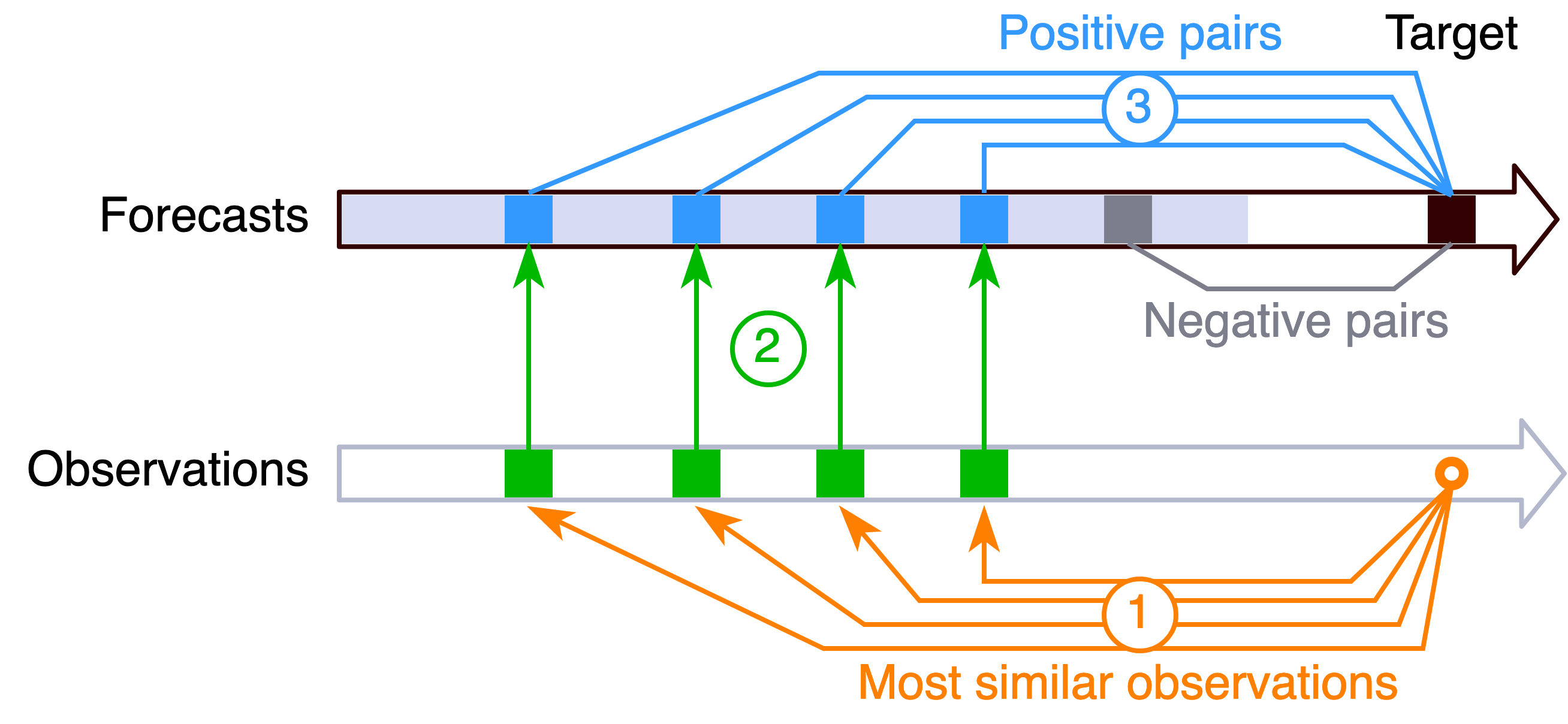
Figure 2: Schematic for identifying reverse analogs during the triplet sampling from historical forecasts and observations

Figure 2 shows the schematic for the reverse analog process. It echos the AnEn schematic presented in Hu and Cervone’s paper but the direction of information flow has been reversed for the specific purpose of optimization. To identify which forecasts should be truly more similar than others, we refer to the corresponding observation field. In other words, similarity of forecasts is determined not from forecasts per se, but rather from the corresponding observations. If the associated observations are very similar, the corresponding forecasts are deemed analogs, although the original Euclidean distance calculated directly from forecast variables might be large. And this is indeed the additional information the triplet network aims to learn: the forecast error patterns coupled with certain types of observation values. Specifically, the reverse analog technique works as follows:

1. Most similar historical observations (green rectangles) to the current observation (orange circle) are found.

2. The associated historical forecasts (blue rectangles) are queried.

3. The current target forecast (black rectangle) is deemed to be more similar to the matched historical forecasts (blue rectangles) than other unmatched historical forecasts (grey rectangle).

One might argue that similar observations might not necessarily indicate actual similar weather patterns. The degree of freedom is hard to control, subject to seasonality, diurnal variability, and random variation. We offer two counterpoints in this light: (1) similar forecasts and observations are sought independently at each location and each forecast lead time which would control for spatial and diurnal variability; (2) we incorporate a fitness proportionate selection stage [47, 48] to introduce randomness and to prevent greedy search [49, 50, 23]. The goal is not to distinguish every nuance of the observational difference, but to learn an effective embedding function relating forecast errors and observations.

3 Research Datasets

Experiments have been carried out at two geographic scales to show the effectiveness of using a ML driven similarity metric.

The first geographic scale is a small scale study located at Pennsylvania State University. The ground observation station is actively maintained by the Surface Radiation Budget (SURFRAD) project . Observations of solar irradiance and surface wind speed have been collected from SURFRAD between 2011 and 2019. SURFRAD [51, 52] project was established in 1993 to provide high-quality, continuous, and long-term measurements of the surface radiation budget. Observations from SURFRAD have been used in various validation procedures for satellite-derived estimates and NWP models. In our case, the verified NWP model is the North American Mesoscale Model (NAM) forecast system. NAM is one of the major operational models run by National Centers for Environmental Prediction (NCEP) for weather predictions. It uses boundary conditions from the Global Forecast System (GFS) model and is initialized four times per day at 00, 06, 12, and 18 UTC. Each initialization produces forecasts for the next 84 hours. The first 37 lead times are hourly and then the temporal resolution is reduced to every three hours until the maximum lead time is reached. NAM has various grid types each associated with a different spatial resolution. The outer domain with 12-km horizontal grid increments covering the Continental United States (CONUS) is used in this work. NAM provides simulations for over three hundred weather variables that cover a wide range of vertical profile of the atmosphere. It simulates in total 60 vertical layers on a hybrid sigma-pressure coordinate system. It also simulates a single compound atmospheric layer for variables like downwelling shortwave solar radiation and total precipitation. NAM forecasts [53] initialized at 00 UTC from 2011 to 2019 have been collected and subset to the region of Pennsylvania. The closest model grid to the SURFRAD stations is identified. Model forecasts from this grid are verified with SURFRAD stations.

The second geographic scale is a large scale study that covers Pennsylvania. The variables of interest are solar irradiance and wind speed at the surface and 80 meters above ground. Please note that the analysis of wind speed forecasts at 80 meters above ground is omitted in the small scale study because observations are not available from SURFRAD, but it is included in the large scale study because it is the most relevant variable for regional wind power assessment. The NWP model remains to be NAM but SURFRAD observations do not have sufficient spatial coverage of this area, so the model analysis field is used during verification. NAM analysis initialized at 00, 06, 12, and 18 UTC are collected. Model analysis is used as a best-scenario approximation to ground truth where the ground measurements are not available. The state of Pennsylvania is chosen due to its direct closeness to the SURFRAD station. There are in total 1225 grid points in the selected domain.

4 Results

Results for wind speed and solar irradiance predictions are organized into several sections. All experiments have the same test period of 2019. The training period for the ML model and the search period of AnEn are both from 2011 to 2018 to ensure a fair comparison, except for Section 4.3 where the length of search is of particular interest. All experiments have 11 members in forecast ensembles.

There are two configurations of AnEn that are treated as baselines. The first configuration is the optimal AnEn. This configuration is deemed optimal in a sense that the predictors used are selected based on literature [6, 1, 25, 14, 4] and the respective weights are then optimized via an extensive search that tests for all possible combinations of weights with an increment of 0.1 from 0 to 1. The selected predictors include downwelling shortwave radiation, surface wind speed and wind direction, relative humidity and temperature at 2 meters above ground.

The second configuration is the equal weighting scheme, namely the equally weighted AnEn. This configuration uses the same predictors as the ML model. There are in total 227 variables selected from NAM for both the equal weight scheme and the ML model. Several variables are excluded from the training process due to being soil attributes, not necessarily related to atmospheric conditions. Due to the sheer number of variables, an extensive search would not be possible and therefore, equal weighting is the next most practical thing to do.

We trained two separate ML models, one for wind speed predictions and one for solar irradiance predictions, with both following the same model architecture. The LSTM embedding network has 20 hidden features and three hidden layers. In other words, 383 predictors are transformed into a 20-dimensional space which is then used to identify analogs. These hyper-parameters are decided based on several trials with 3, 5, 20, and 50 hidden features and 1, 2, and 3 hidden layers respectively. The maximum training iteration is 200,000 and early stopping is engaged to prevent model overfitting. In the rest of the description, predictions generated from the ML driven similarity metric will be referred to as Deep Analog (DA) for simplicity.

4.1 Weight Optimization

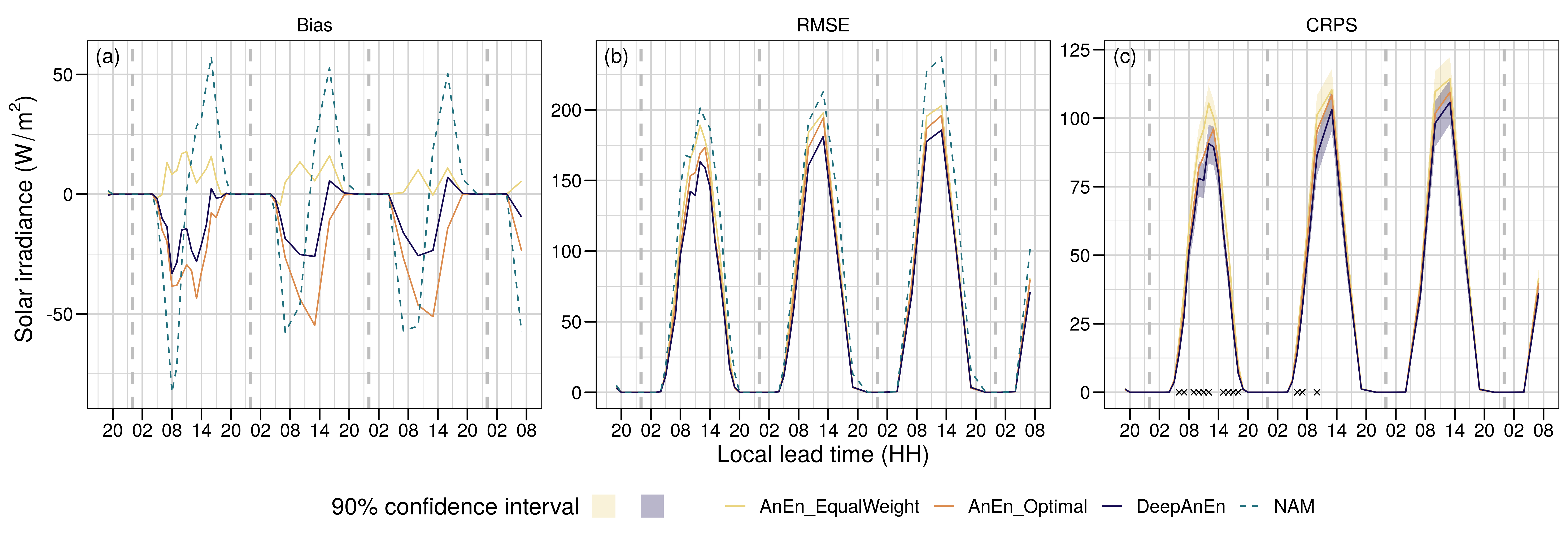
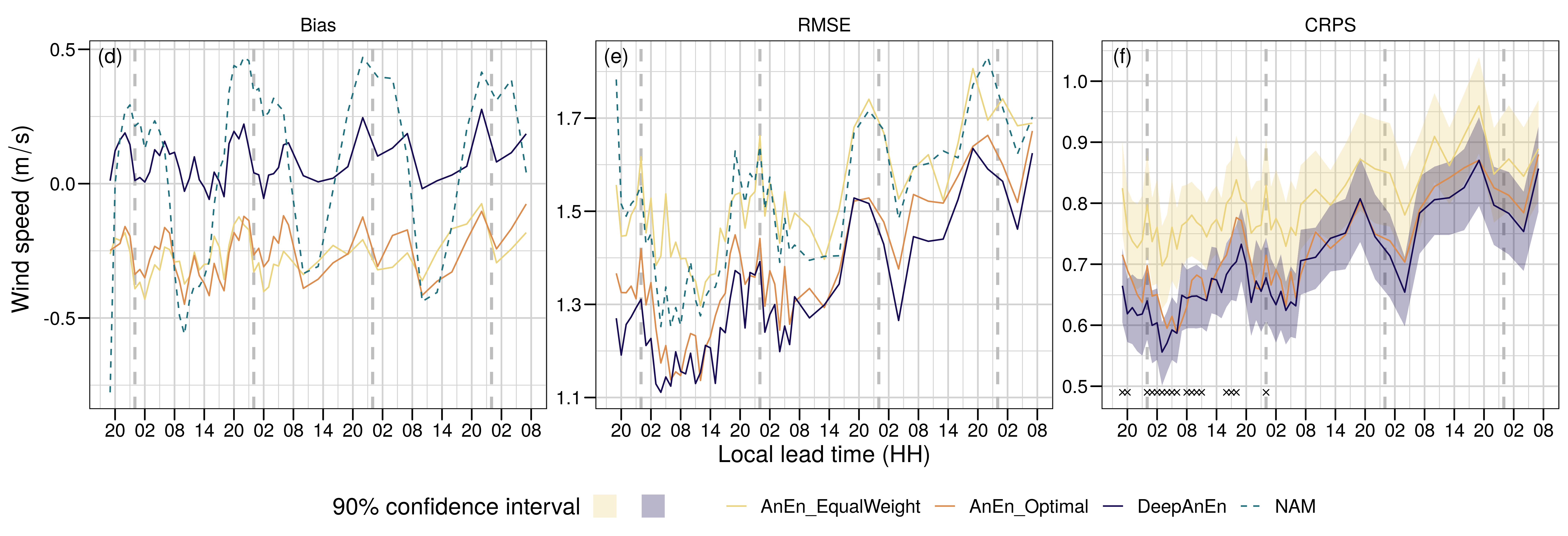
Figure 3: Verification comparisons for (a, b, c) solar irradiance and (d, e, f) wind speed forecasts. Black crosses on the bottom of (c, f) indicate the lead time hours that DA is significantly better than AnEn with equal weighting at a 90% confidence level. Vertical dashed lines indicate individual forecast days.

Figures 3 (a, b, c) show the bias, Root Mean Square Error (RMSE), and CRPS for solar irradiance forecasts. Overall, based on comparisons of RMSE and CRPS, DA outperforms all other methods. Specifically, DA significantly outperforms the equally weighted AnEn for most of the lead times in the first 24 hours. This time period, namely the day-ahead horizon, is of particular interest in terms of the energy market bidding and it is important for energy system planning and scheduling that tries to match power demand and supply. From the bias panel, NAM demonstrates a negative bias during mornings and a positive bias during afternoons. This suggests that NAM has problems simulating the exact diurnal trend. All configurations of AnEn have been able to correct this behavior but they produce slightly different results. The equally weighted AnEn shows a positive bias while the optimal AnEn shows a negative bias possibly caused by giving a dominant weight on downwelling shortwave radiation and then taking the average of the ensemble members. DA achieves better bias than the optimal AnEn for almost all lead times. This indicates that by using the transformed features from many more predictors, DA is able to find better analogs that are missed by the optimal AnEn. Although all configurations of AnEn still produce bias, the bias magnitudes are very small compared to other error statistics, like RMSE and CRPS.

Verification on wind speed predictions demonstrates similar results, shown in Figures 3 (d, e, f). DA is shown to outperform both the optimal AnEn and the AnEn with equal weighting for most of the forecast lead times on average for RMSE and CRPS. DA is significantly better, in CRPS, than the equally weighted AnEn for most of the lead times in the first 24 hours. These results are consistent with the verification on solar irradiance predictions. It should be noted that the RMSE of the equally weighted AnEn has degraded to the level of NAM for most of the lead times when predicting wind speed. This suggests that simply increasing the number of predictor variables does not guarantee an improved accuracy. Bias-wise, DA clearly achieves better bias than all other methods. NAM has a similar problem, as in Figure 3 (a), in simulating the diurnal changes in wind speed resulting to a sine wave-like bias diagram. By average, the equally weighted AnEn has a bias of -0.271 $m/s$ and the optimal AnEn has a bias of -0.260 $m/s$. DA is able to reduce the bias to an average level of 0.080 $m/s$.

In terms of significance level, DA remains significantly better than the equally weighted AnEn for most of the lead times in the first forecast day period at a 90% confidence level. This suggests the effectiveness of ML model training as a weight optimization process.

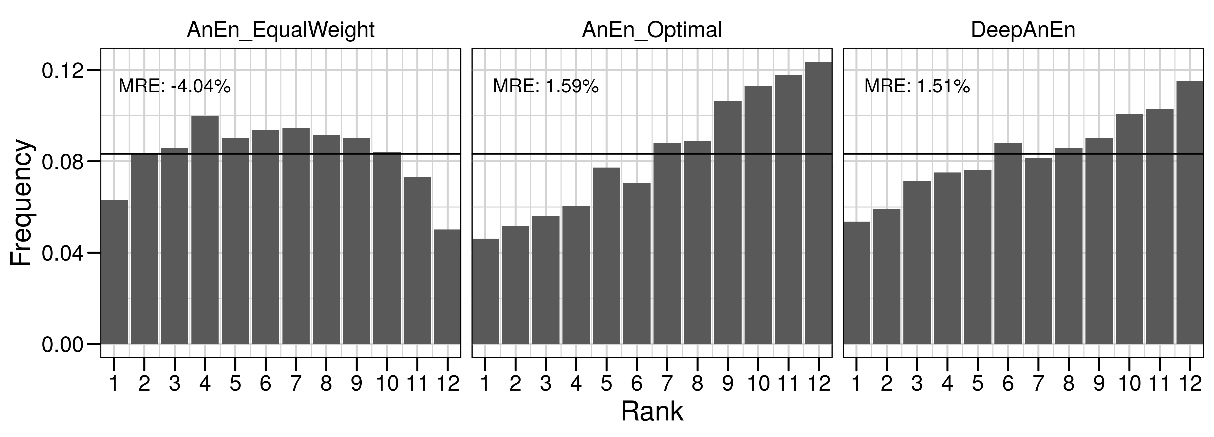
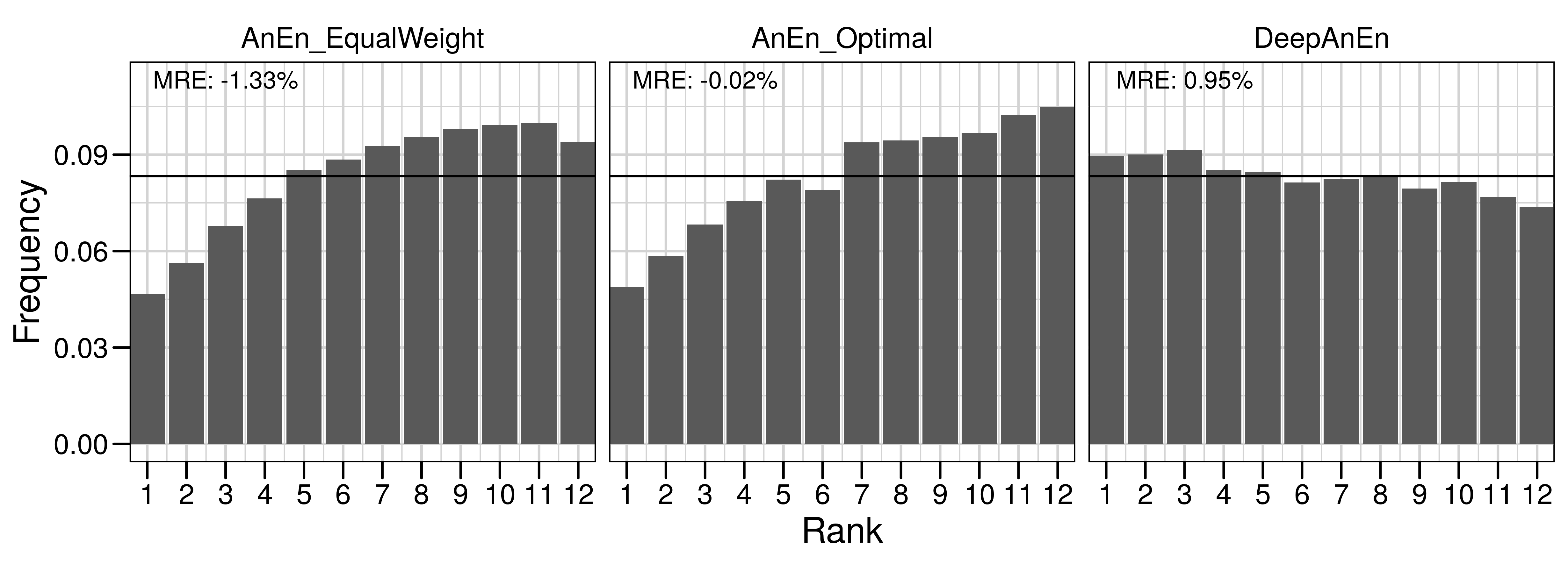
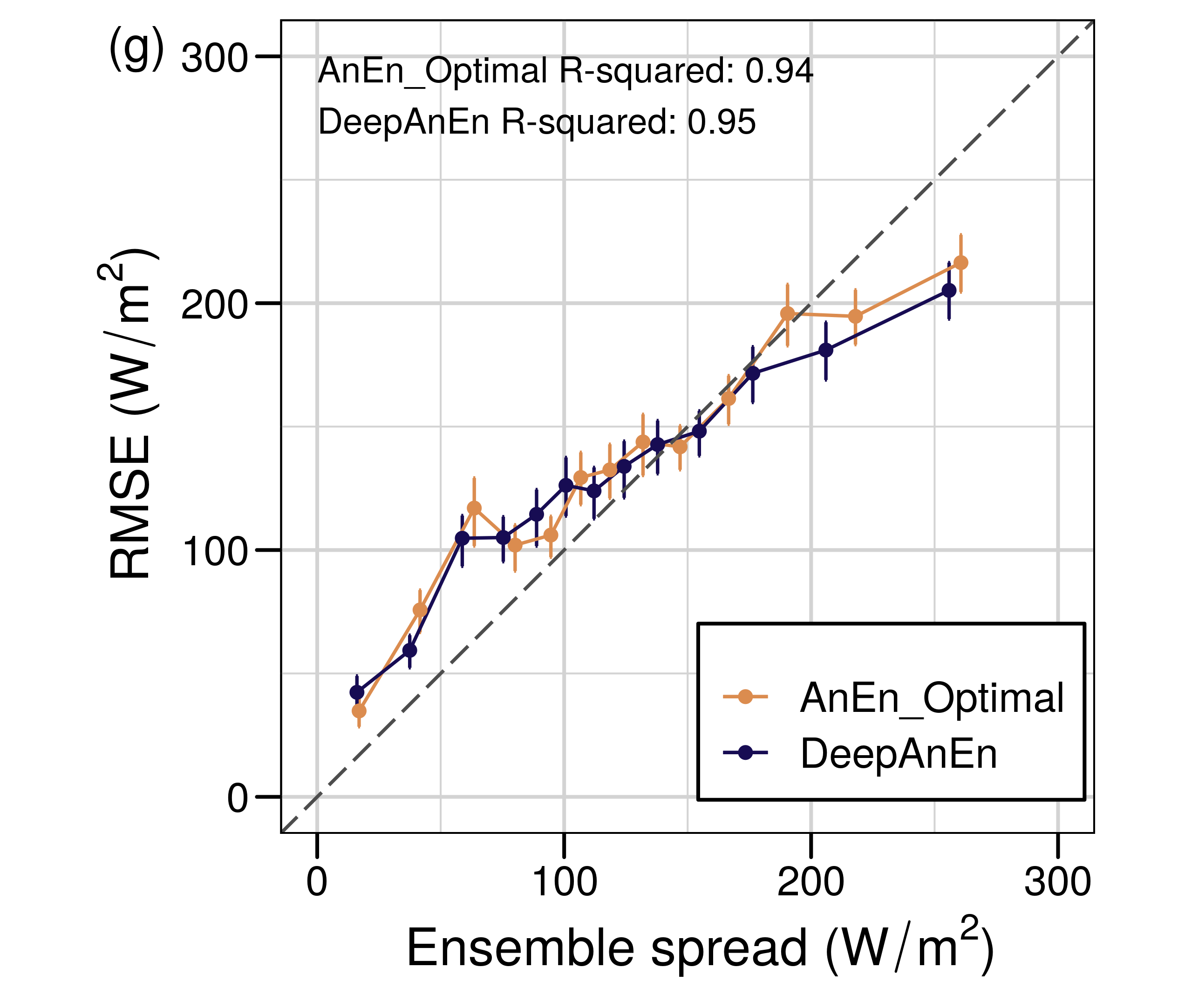
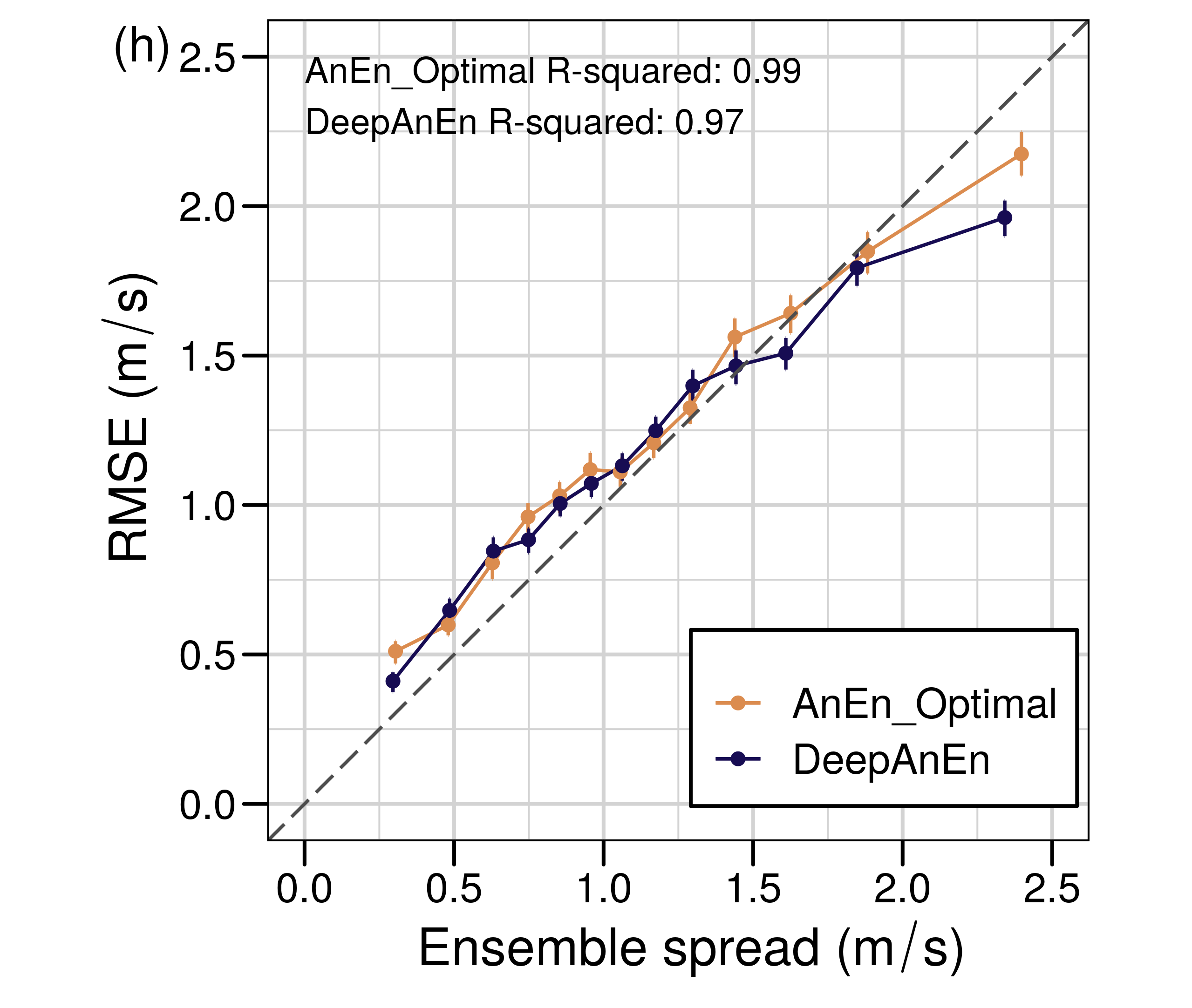
Figure 4: Rank histograms and reliability diagrams for solar irradiance and wind speed forecasts. (a, b, c) and (d, e, f) show the rank histograms respectively for solar irradiance and wind speed forecasts with 11 ensemble members across all lead times. (g) and (h) show the binned spread-error relationship diagrams respectively for solar irradiance and wind speed forecasts. RMSE is used as the error measure on the vertical axes in (g, h). Vertical lines on each dot indicate the 90% confidence interval.

Next, the statistical consistency and the spread-skill relationship of DA and AnEn are evaluated with rank histograms and binned spread-error diagram, respectively, as shown in Figure 4. Figures 4 (a, b, c) show the rank histograms for solar irradiance forecasts. The ensembles from equally weighted AnEn is slightly over-dispersed, or under-confidence, confirmed by a negative MRE and a convex shape of the rank histogram. When using all available variables without discrimination, weather analogs that are actually associated with the variable of interest are hard to find and as a results, the ensemble spread tends to be too large. Both DA and the optimal AnEn produce slightly under-dispersed ensembles as indicated by a positive MRE while DA is closer to zero than AnEn. The prevailing positive slope in both rank histograms confirms the systematic low bias shown in Figure 3 (a). Figures 4 (d, e, f) show the rank histograms for wind speed forecasts. Consistent with Figure 3 (d), DA successfully reduce biases in other two configurations of AnEn by yielding an almost flat rank histogram. Its MRE is still positive indicating ensembles being slightly under-dispersive. The ensemble characteristics of the two configurations of AnEn are highly similar, both having a negative bias and over-dispersive ensembles.

The spread-error diagram, shown in Figures 4 (g, h), quantifies the ability of the ensemble in estimating the prediction errors. Forecasts from DA and the optimal AnEn have very similar ability to quantify uncertainty except for ensembles with a larger spread (right tails). DA is able to reduce errors while hardly impacting the spread for ensembles with a spread that is larger than 180 $W/m^{2}$ and 1.8 $m/s$. The slightly lower R-squared measure is primarily caused by the right tails of DA correlation deviating further from the diagonal line than the optimal AnEn. This indicates that DA carries out a shift to the forecasted distribution to the correct direction without changing the shape of the distribution. It is worthwhile to note that DA achieves similar performance as the optimal AnEn in most cases but they start to become different when looking at the hard-to-predict cases that are associated with larger errors. Some examples of such hard-to-predict cases include: (1) abrupt weather regime changes, and (2) constantly moving partial clouds. This difference will be further discussed in the following section.

4.2 Relationship between Performances and Training Length

Results from Section 4.1 have shown that the triplet network with an LSTM embedding is able to learn an effective transformation function from over hundreds of predictor variables down to twenty latent features. Overall, DA outperforms the optimal AnEn. Since the cases where differences exist between the two methods likely lies within the hard-to-predict scenarios, as shown in Figures 4 (g, h), this section focuses on comparing the ability of two methods in correcting the underlying NAM when it is making larger errors.

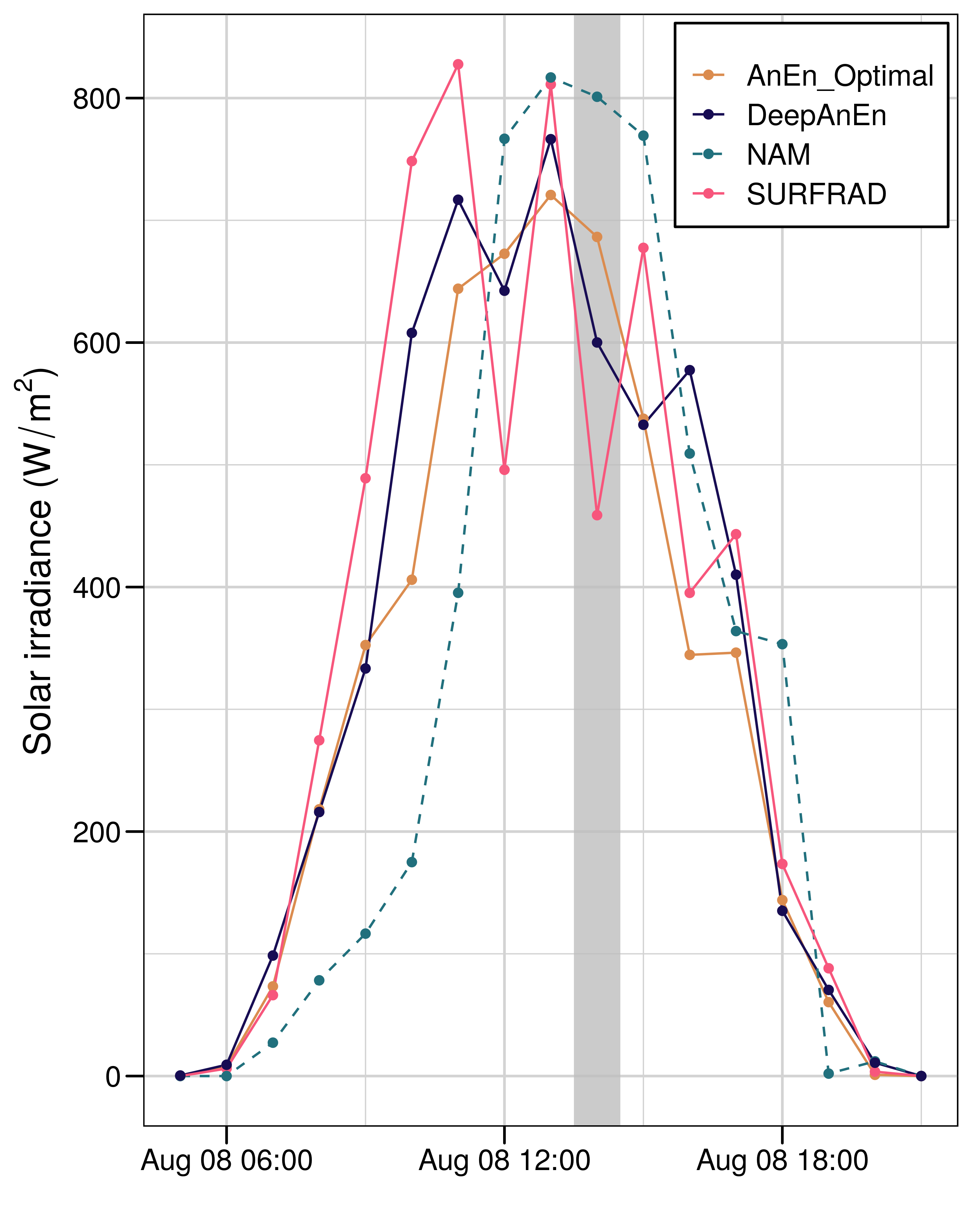
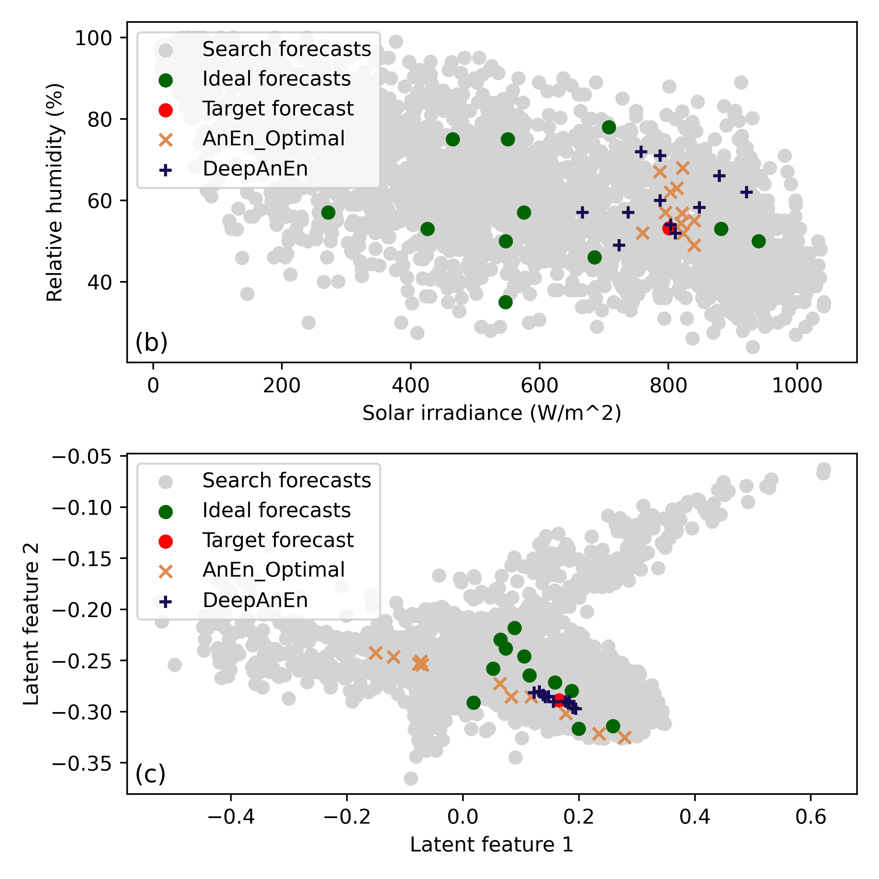
Figure 5: A case study of solar irradiance prediction on August 8th, 2019, showing the predicted time series from various methods (a). The average of ensemble members are calculated to show a single predicted time series. The shaded area is 2 PM location time. A subset of the original forecast variables and the latent features at this particular time point are shown in (b) and (c).

First, let’s consider a case study of solar irradiance prediction on August 8th, 2019. Figure 5 (a) shows the observed and predicted time series from NAM, and the ensemble mean of DA and the optimal AnEn. SURFRAD time series shows a bumpy temporal trend with a large amount of variation from the late morning to the early afternoon. The average irradiance during noon, however, is around 600 $W/m^{2}$ which amounts to a typical semi-cloudy day. The large variation is likely attributable to the passage of clouds over the sites that alternate with clear-sky periods. This type of sky condition is particularly hard for a medium-range forecast system, like NAM, to simulate and predict. In fact, NAM does not capture well the cloud dynamics on this particular day, producing a smooth time series peaking at 800 $W/m^{2}$, which corresponds to an irradiance value in the lower end of the distribution associated with clear-sky conditions. The optimal AnEn is able to compensate for the high bias of NAM predictions, leading to an increase in the prediction variability around the averaged observed value, although the observed variance still appears to be underestimated. DA, on the other hand, is able to reconstruct the observed temporal variability and to better correct NAM.

To better understand the method’s performances, Figures 5 (b, c) shows a subset of the original forecast variables and the latent features learned by DA at 2 PM on August 8th, 2019, denoted by the shaded timestamp on Figure 5 (a). The optimal AnEn uses five predictors while DA uses all 227 predictors available. Due to the limit of visualization, only solar irradiance and surface relative humidity are plotted in Figure 5 (b) from the original forecast variable space; only the first two latent features are plotted in Figure 5 (c) from the transformed latent space. The grey dots indicate all the historical forecasts in the search repository from 2011 to 2018 and they collectively show the distribution of these historical forecasts in the two-dimensional space. The target forecast, namely the NAM forecast valid at 2 PM on August 8th, 2019, is shown as a red point. The historical forecasts selected by optimal AnEn are denoted as orange crosses and the historical forecasts selected by DA are denoted as blue pluses. The ideal members are the historical forecasts selected by the reverse analog process, denoted as green dots. These members are ideal in the sense that the corresponding observations to these forecasts will produce the most accurate predictions. In other words, these forecasts are associated with the observations that are closest in values to the true solar irradiance value (at around 460 $W/m^{s}$). An ideal analog similarity function would lead to selecting these 11 green dots as weather analogs, and then the resulted ensemble would center around the true value with a sharp distribution.

It is clear in the original forecast variable space, as in Figure 5 (b), the green dots are scattered across different regions of the forecast distribution. Because a Euclidean distance is used to define similarity, the optimal AnEn selected dots that are closest to the target forecast in the original space. Note that it might not seem as obvious from the figure because only two dimensions are plotted. In practice, there are five dimensions for the optimal AnEn. This inability to choose good analogs could be caused by not having enough examples in the training for the standard AnEn algorithm, or that the metric or the selected set of predictors is not optimal. However, as shown in Figure 5 (c), DA first transformed the variable space into a 20-dimensional latent space, and then selected the closest candidates. Although none of the green dots (the ideal forecasts) are actually selected as analogs, they are much more clustered around the target forecast compared to the original space, making them more likely to be selected. This is likely the result of adopting an improved metric and set of predictors. Indeed, the difference in the similarity metric leads to the result that weather analogs selected by the optimal AnEn are further apart in the latent space while the weather analogs selected by DA are further apart in the original forecast variable space. This difference in the analog selection behaviors is causing the differences in the final predictions. It indicates that additional knowledge has been ingested into the transformation function employed by DA. The improved performance benefits from the training stage of the triplet network with a reverse analog procedure. Similar behaviors have also been observed in wind speed predictions (not shown).

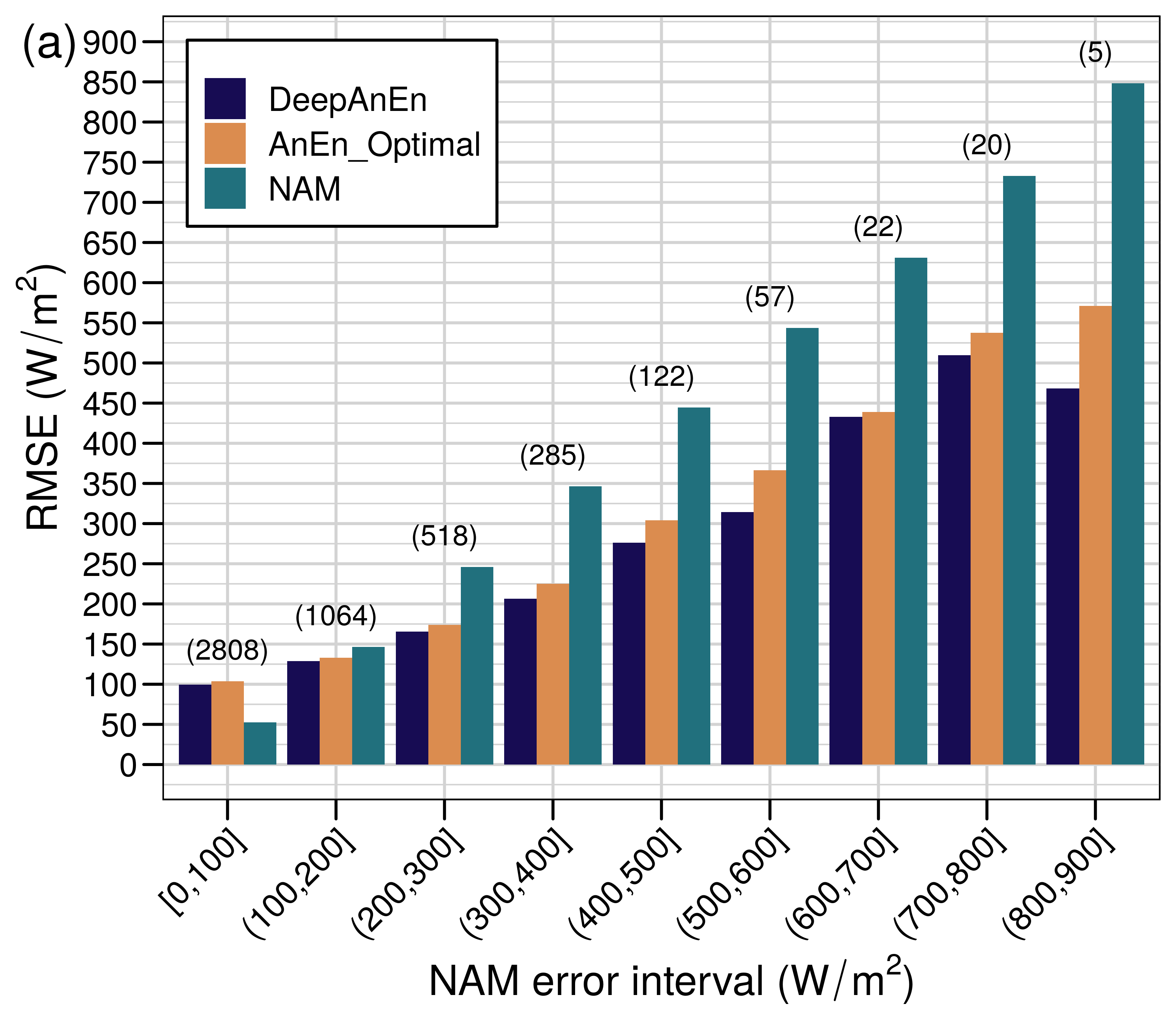
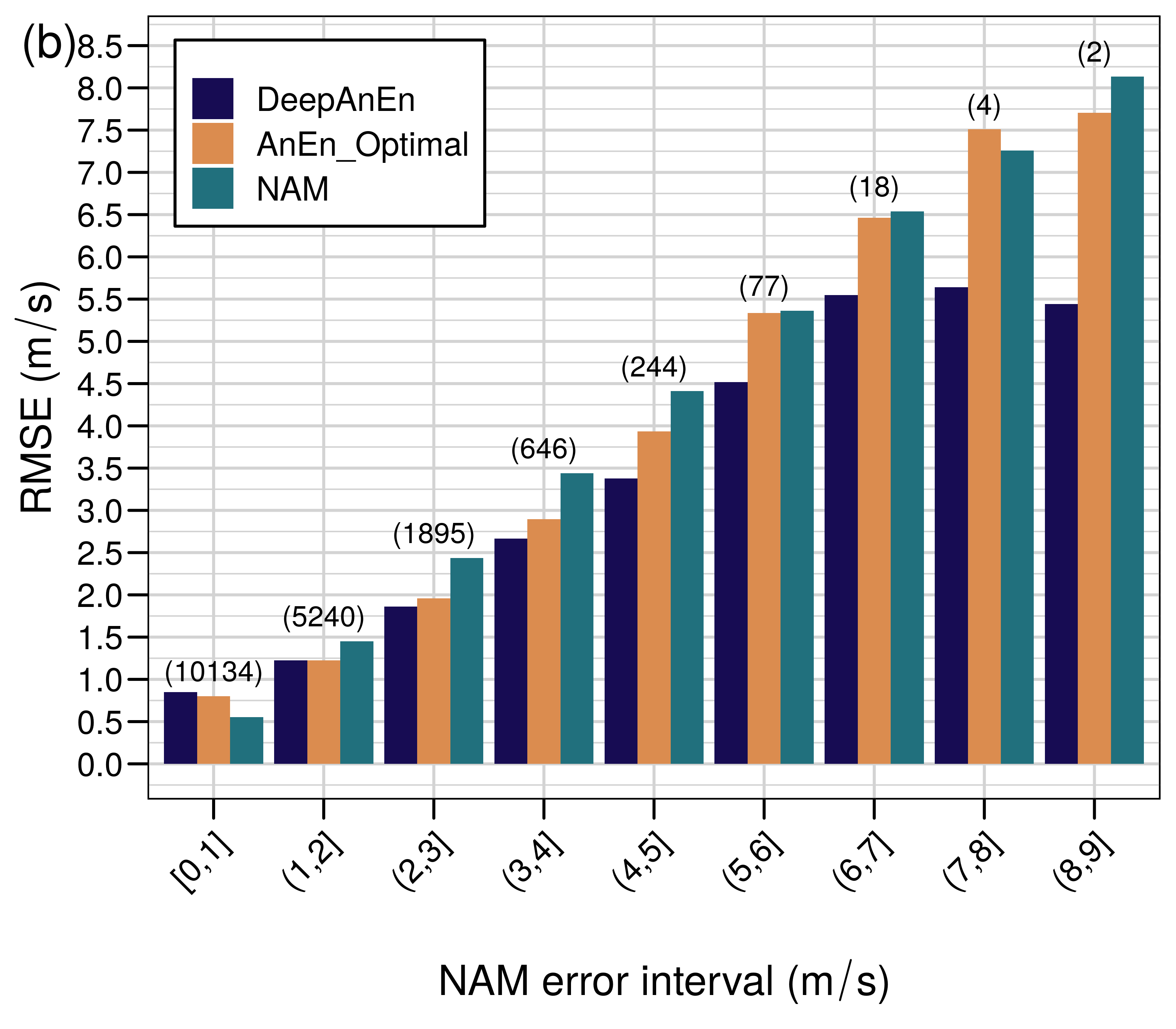
Figure 6: RMSE for (a) solar irradiance and (b) wind speed forecasts binned with NAM prediction error intervals. Verification for wind speed forecasts are done for all forecast lead times; verification for solar irradiance forecasts are only done for lead times valid during day times to prevent possible skewing of the results. The number on top of each bar group denotes the total number of forecasts verified in the particular error interval group.

To quantify the ability of DA and the optimal AnEn in reducing errors of different magnitudes, NAM predictions are binned based on their individual forecast error. Figure 6 shows the RMSE summary for solar irradiance forecasts. It is clear that analog-based ensemble techniques improve NAM for all error intervals except for the lowest ones. At the same time, DA consistently demonstrate greater capability of error correction compared to AnEn, indicating by a smaller RMSE compared to AnEn. Similar results can be observed from Figure 6 on wind speed predictions. While the improvement from NAM to AnEn is not as great as in the case of solar irradiance predictions, DA consistently offers better error correction to NAM compared to AnEn, leading to a lowest RMSE, except for the lowest error interval group. Interestingly, neither analog-based ensemble technique beats the underlying NAM model in the lowest error interval. This indicates that, if NAM already provides an accurate deterministic prediction, the analog-based ensemble technique might decrease, rather than further increase, the prediction accuracy.

In summary, using more variables with an ML driven similarity metric while identifying weather analogs has the advantage to correct predictions for cases where the underlying NWP model produces significant errors, as shown by DA greater ability to correct larger errors than the optimal AnEn. This has a great implication for its application to hard-to-predict events where the NWP model fails and the conventional AnEn has been found to produce a systematic bias [25].

4.3 Effect of Model Updates

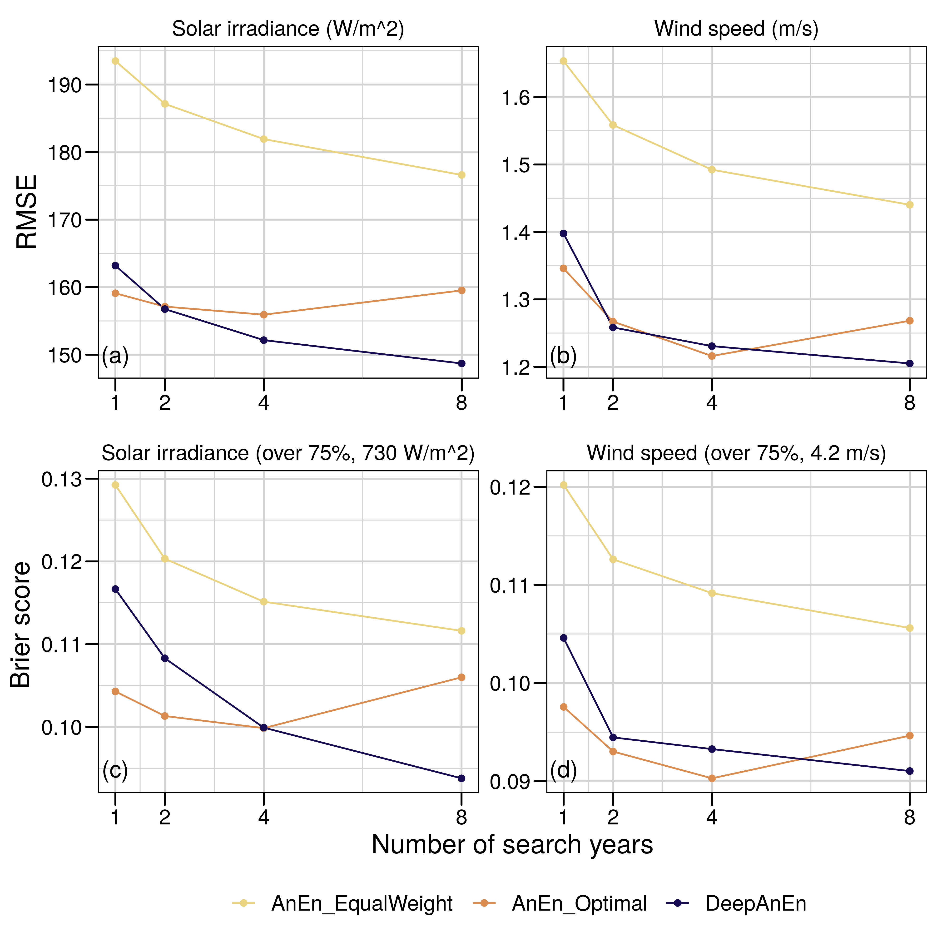
Figure 7: Sensitivity studies of the length of historical search repository for predicting solar irradiance and wind speed. Historical forecasts from 2018 are used for the single-year case; forecasts from 2017 to 2018 are used for the two-year case; forecasts from 2015 to 2018 are used for the four-year case; and forecasts from 2011 to 2018 are used for the eight-year case. (a, b) show the RMSE and (c, d) show the Brier scores. The performance metrics are generated from a subset of lead times (11 AM to 12 PM) to prevent skewed verification due to night times. Weights used by the optimal AnEn are optimized using the eight-year case; the embedding network used by DA is trained with the eight-year case.

It is often assumed that better weather analogs can be found with a longer repository of historical forecasts, particularly for less frequent events. This assumption, however, can be violated whenever there are updates to the underlying NWP model, which can potentially pose a limit on the performance of any postprocessing method built on that model. Depending on the nature of the updates, a long historical search repository of an operational model might not be as useful as one would initially expect. This section focuses on sensitivity of the length of the historical search repository and its impact on prediction errors.

NAM has been constantly updated with major and minor changes. The most important change was an update of its core from the Eta model to the Weather Research and Forecasting (WRF) model in 2006. After that, NAM has had roughly a minor update every several months . There is currently little information on how tolerant AnEn is in terms of model updates. Part of the reason lies within the intrinsic difficulty in quantifying the tolerance because the impact of a model update on the model itself can be highly complex and sometimes even unknown. Quantifying the impact on AnEn performance would add another layer of complexity.

This paper shows results using two common metrics, RMSE and the Brier score, comparing the performance of analog-based methods with different lengths of search repository. Results do not focus on causal relationship but only examine the sensitivity of various analog-based methods.

Figures 7 show the verification for solar irradiance and wind speed predictions with different numbers of historical years in the search repository. The Brier score quantifies how well the analog-based methods predict an event over the 75%-percentile value of the observed distribution. This 75%-percentile value corresponds to 730 $W/m^{2}$ in irradiance and 4.2 $m/s$ in wind speed. To prevent possible skew of verification since solar irradiance is only abundant during the daytime, results are calculated the local time from 11 AM to 12 PM over the entire test period of 2019.

All four panels in Figure 7 demonstrate a similar pattern when increasing the number of historical years in the search repository. The optimal AnEn (orange solid line) has a “saturation point” at around four years where it then stops decreasing its forecast errors given more historical forecasts. Its error starts to increase given more than four years of historical forecasts. Interestingly, the equally weighted AnEn with 227 input forecast variables, shown in solid yellow lines, continues to decrease when more historical data are added, although the error remains high. DA, shown in solid blue lines, has a similar pattern that continues to decrease forecast errors given more historical forecasts while achieving significantly better results than the equally weighted AnEn. The consistent trend of the error decreasing for DA suggests that it is able to account for more degrees of freedom in the forecasts and that additional data allows to find more robust latent features throughout multiple years even when the NWP model has gone through routine updates. However, it is not definitive that the “saturation point” for regular AnEn is at four years because the magnitude of error changes is relatively small. It has only been 11 years since NAM changed its model core in 2009, so a longer data repository from a different model is needed to study this problem in a more conclusive fashion.

4.4 Prediction Spatial Patterns

Previous sections have evaluated the three analog-based methods (DA, the optimal AnEn, and the equally weighted AnEn) at Pennsylvania State University. To investigate the effectiveness of DA on a spatial domain, this section extends the geographic scale from Pennsylvania State University to the entire region of Pennsylvania. The area of Pennsylvania, consisting of 1225 grid locations, is selected for its direct vicinity to our previously studied area. Analogs are sought independently at each location and the ML models are trained with the same architecture. Prediction errors are calculated with regard to NAM model analysis initiated at later forecast cycles, 1800 UTC, due to the lack of a continuous spatial coverage from SURFRAD networks. RMSE is average across the test period of August 2019, and four forecast lead times valid at 2, 3, 4, 5 PM local time. This is primarily to test the performance during daytime when larger variations in both solar irradiance and wind speed are to be expected.

Experiment	Predictand	Vertical Level	Trained ML Models	Training Data Sites
1	Solar irradiance	Surface	1	1
2	Solar irradiance	Surface	1	100
3	Wind speed	Surface	1	1
4	Wind speed	Surface	1	100
5	Wind speed	Surface	8	408
6	Wind speed	80 meters above ground	1	1
7	Wind speed	80 meters above ground	1	100
8	Wind speed	80 meters above ground	9	408

Table 1: A summary of experiments for training configurations of ML models for spatial predictions of DA

Variable	Configuration	Average RMSE (Min / Max)	Improvement (%)
Solar irradiance ($W/m^{2}$)	NAM	158.02 (136.59 / 182.06)	*
	AnEn_EqualWeight	162.43 (145.33 / 182.16)	-2.79
	AnEn_Optimal	133.66 (119.47 / 151.88)	15.42
	DeepAnEn 1 @ 1	136.63 (120.87 / 161.42)	13.54
	DeepAnEn 1 @ 100	130.31 (111.24 / 148.01)	17.54
Surface wind speed ($m/s$)	NAM	0.81 (0.61 / 1.12)	*
	AnEn_EqualWeight	1.06 (0.78 / 1.68)	-30.76
	AnEn_Optimal	0.75 (0.54 / 1.07)	7.56
	DeepAnEn 1 @ 1	0.83 (0.64 / 1.62)	-2.62
	DeepAnEn 1 @ 100	0.68 (0.51 / 1.07)	15.74
	DeepAnEn 8 @ 408	0.7 (0.52 / 1.09)	13.27
80-meter wind speed ($m/s$)	NAM	1.09 (0.91 / 1.46)	*
	AnEn_EqualWeight	1.46 (1.16 / 2)	-34.08
	AnEn_Optimal	1.01 (0.81 / 1.32)	7.47
	DeepAnEn 1 @ 1	1.09 (0.87 / 1.8)	0.00
	DeepAnEn 1 @ 100	0.94 (0.77 / 1.33)	13.21
	DeepAnEn 9 @ 408	0.95 (0.75 / 1.33)	13.07

Table 2: A summary of results from various methods. DeepAnEn 1 @ 1 represents DA predictions with 1 ML model trained with data from 1 site.

Table 1 summarizes the different configurations of ML models for spatial predictions of DA. A series of experiments have been carried out specifically to investigate

1. the performance of DA on three weather variables,

2. the impact of including more training data from nearby locations,

3. and the potential benefit of training more than one ML model for DA.

When only one training data site is used (Exp. 1, 3, and 6), the model grid closest to the SURFRAD station at Pennsylvania State University is used. The ML model is trained using data from only this grid point and then applied to the entire Pennsylvania. When 100 training data sites are used (Exp. 2, 4, and 7), these sites are equally spaced across Pennsylvania. Exp. 5 and 8 have used a total of 408 training data sites and trained several ML models. The sites and the number of models are determined as follows: the annual wind speed for each grid point is first calculated and then, all grid points are classified and binned with a 0.5 $m/s$ interval; for each interval, an ML is trained using data from the model grids belonging to this interval. Due to the machine memory limit, the maximum number of training data sites for a particular ML is 100. When the total number of grid pints belonging to a particular interval exceeds this limit, 100 sites are randomly selected from the grid points.

Table 2 shows the average RMSE from various forecast methods across the entire domain. The test period is 2019 daily from 2 to 5 PM. The night time is excluded from the verification period because of the reduced variation and amount of solar irradiance and wind speed during nights. Verification of the entire daytime period is unfortunately impossible because, due to data management and archive limit, NAM does not provide the analysis field for a continuous daytime verification. Wind speed verification is carried out for strong wind cases ($>4m/s$). For all three variables, the equally weighted AnEn generally has a higher error than the baseline NAM predictions. This is because weight optimization is essential to the performance of the AnEn technique. In the cases of the optimal AnEn, when the number of predictor variables has been reduced and the respective weights have been optimized using historical data, the average RMSE shows consistent drops compared with the baseline NAM predictions, 15.42% for solar irradiance, 7.56% for surface wind speed, and 7.47% for 80-meter wind speed. When comparing DA and the optimal AnEn, the single ML model trained on 100 equally spaced sites consistently yields the best results, having the lowest RMSE out of all alternative forecasts. When comparing multiple configurations of DA, the ML models trained on 100 locations are generally superior to the models trained on a single location. However, the expected improvement from using a mixture of ML models (DeepAnEn 8 @ 408 and DeepAnEn 9 @ 408) is not observed for wind speed predictions. In these experiments, when more than one ML model is used by DA, each model is responsible of predicting for a subset of the domain that has similar wind speed climatology. This chunking mechanism might be deemed inefficient for choosing the appropriate models. It implies that consuming more computation to train models might not necessarily help to further improve the performance of DA. A different chunking mechanism that divides the domain considering both the physical variable (e.g., wind speed) and orography should be further investigated.

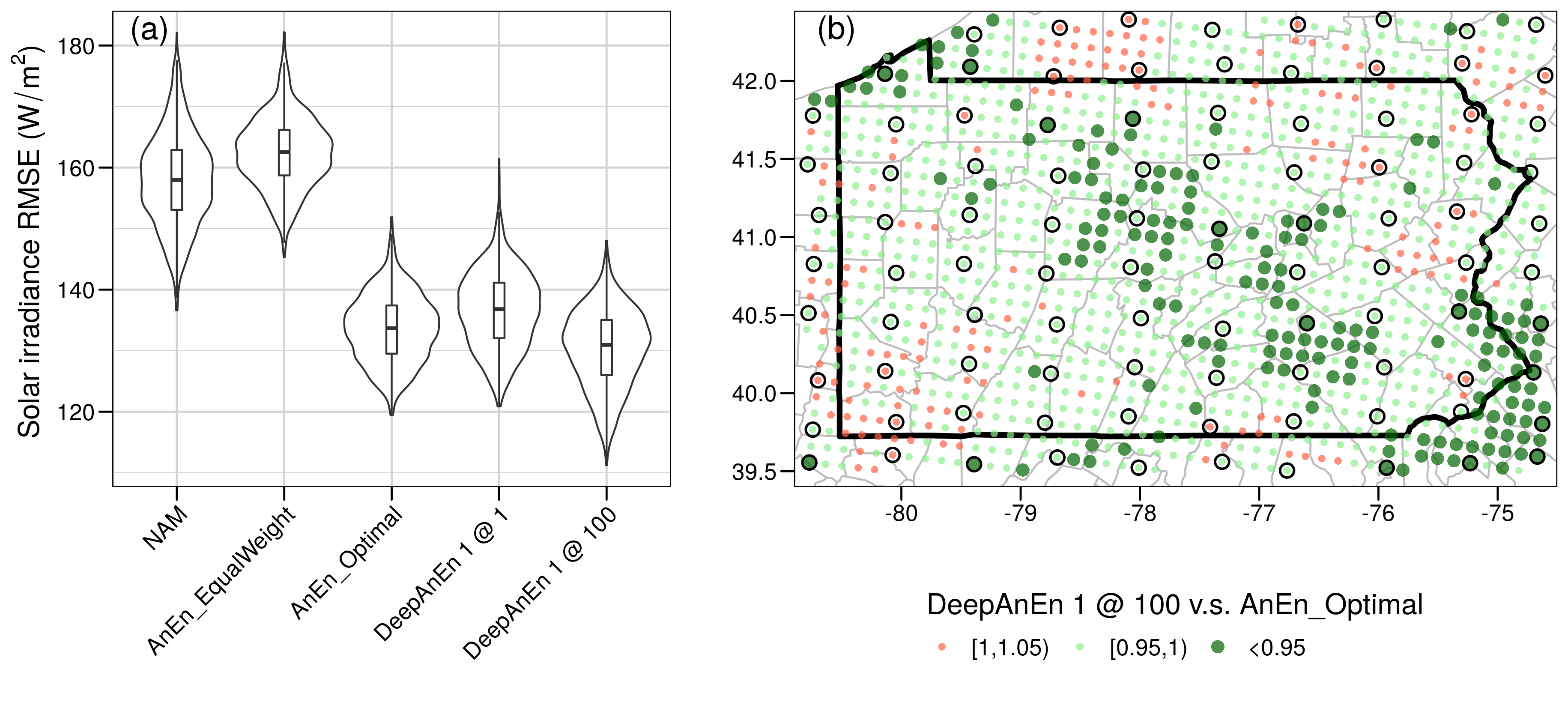
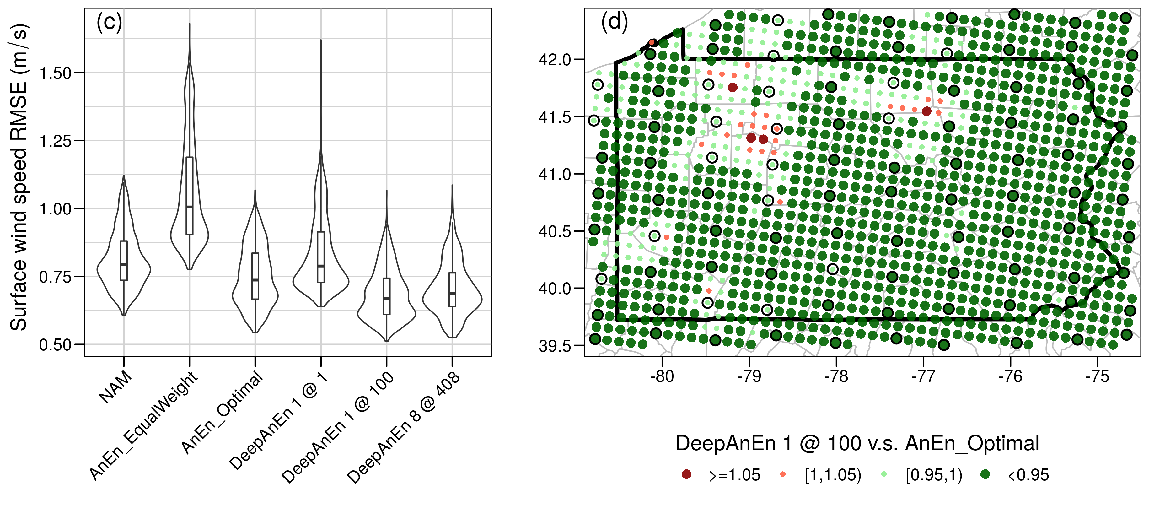
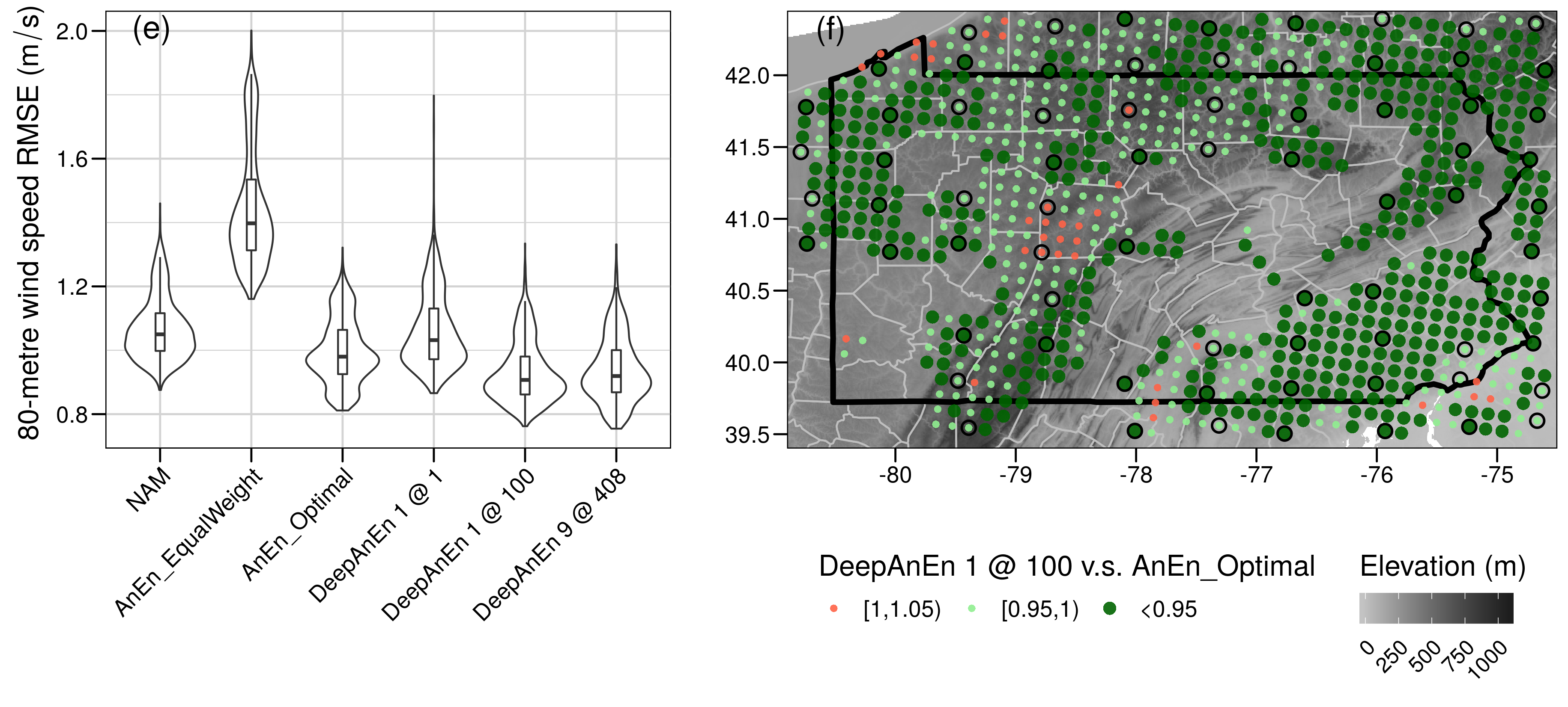
Figure 8: Distributions of prediction errors (a, c, e) and geographic maps comparing DA and the optimal AnEn (b, d, f). The verification period is 2019 daily from 2 to 5 PM to favor the daytime period and only large wind (¿ 4 $m/s$) cases are verified. Predictions over water (upper-left in b, d, f) have been removed to focus predictions on land. In (a, c, e), the three hinges are, in turn, the first, second, and third quartiles; the whiskers extend from the hinge to the value at 1.5 * inter-quantile range of the hinge. Locations with an annual wind speed over 4 $m/s$ are shown in (f) to highlight strong wind region. Training data sites are circled in black.

Figures 8 (a, c, e) show the distributions of prediction errors from different methods and configurations. Figure 8 (a) shows the error distribution of solar irradiance predictions. NAM and the equally weighted AnEn have similar errors while the optimal AnEn and DA show reduced errors. Out of the five methods, DA with 100 training data sites yield the best results. The long tail of large errors produced by DeepAnEn 1 @ 1 suggests that training an ML model using only one data site could lead to a model ignorance on the spatial variation in the domain. This problem can be addressed by increasing the training data and the number of training data sites, as shown by DeepAnEn 1 @ 100. Similar patterns can be observed from Figures 8 (b, c) on wind speed forecasts. Figure 8 (b) shows the the verification on surface wind speed over 4 $m/s$ and Figure 8 (c) shows the the verification on 80-meter wind speed over 4 $m/s$. Again, the equally weighted AnEn failed to improve the baseline NAM model while the optimal AnEn reduces the prediction error. DA with the model trained on 100 data sites doubles the improvements of the optimal AnEn, producing 15.74% for surface wind speed forecasts and 13.21% for 80-meter wind speed forecasts.

Figures 8 (b, d, f) show the geographic maps of RMSE comparing DeepAnEn 1 @ 100 with the optimal AnEn. Green indicates DA has a lower error than AnEn while red indicates DA has a higher error than AnEn. Dots are slightly enlarged when this difference is bigger than 5% of the error of AnEn. The depicted DA uses an ML model trained on 100 locations, circled in black. Figure 8 (f) only shows the verification at the locations where the annual wind speed at 80 meters above ground exceeds 4 $m/s$. These regions are favorable because of the wind abundance and their potential for wind farm investment. The predominant green region shows a consistent outperformance of DA over the optimal AnEn across a spatial domain. DA reduces the prediction error for solar irradiance and wind speed when both resources are abundant temporally and spatially. This indicates DA is suitable as an improved version of AnEn implementation for renewable energy resource forecasts.

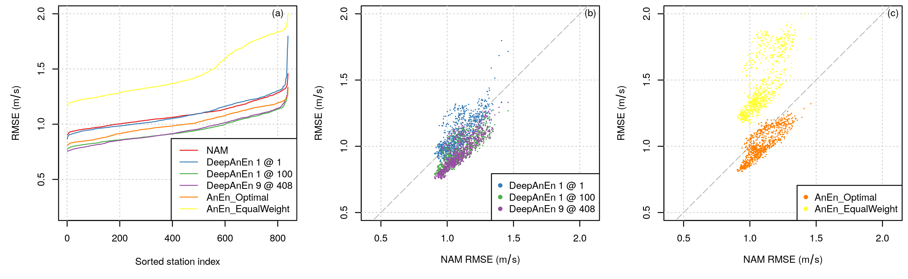
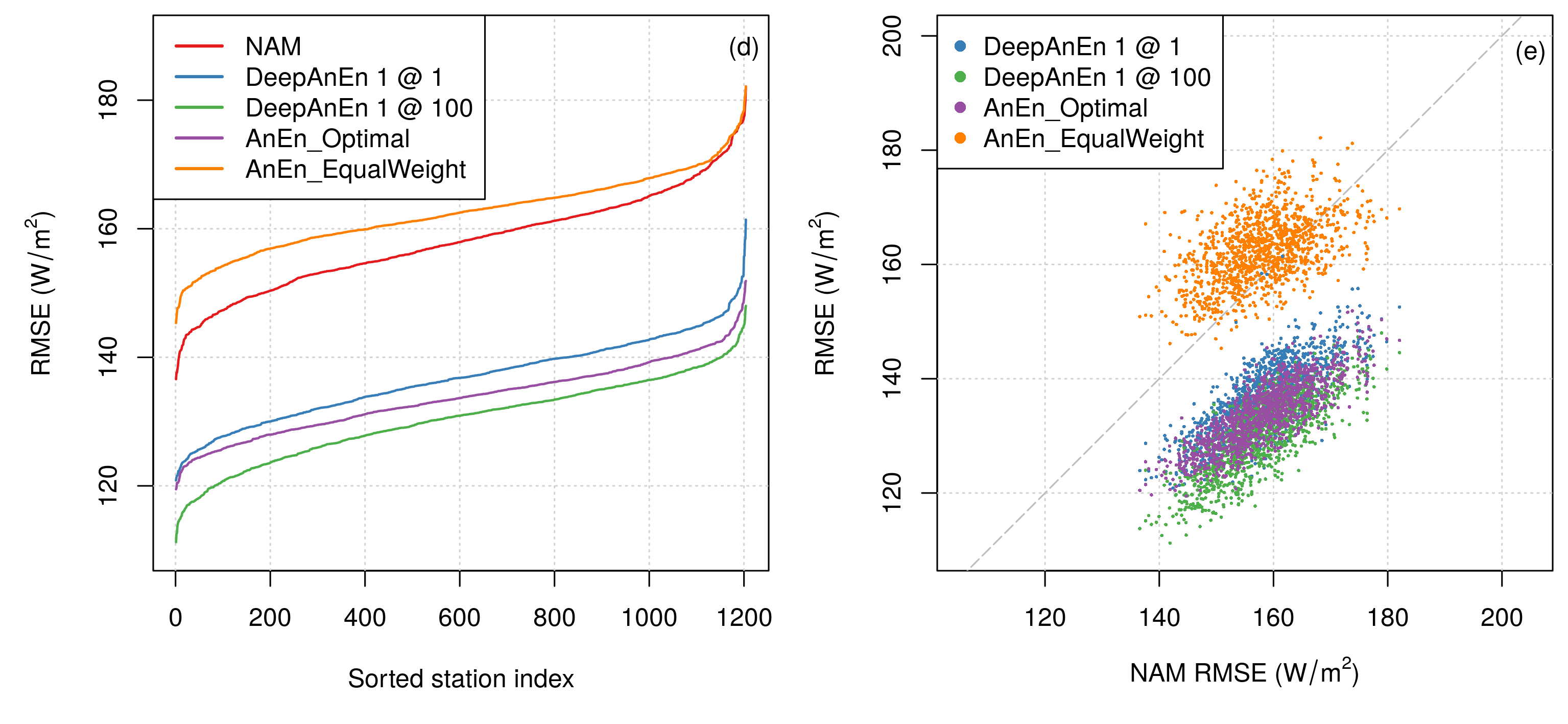
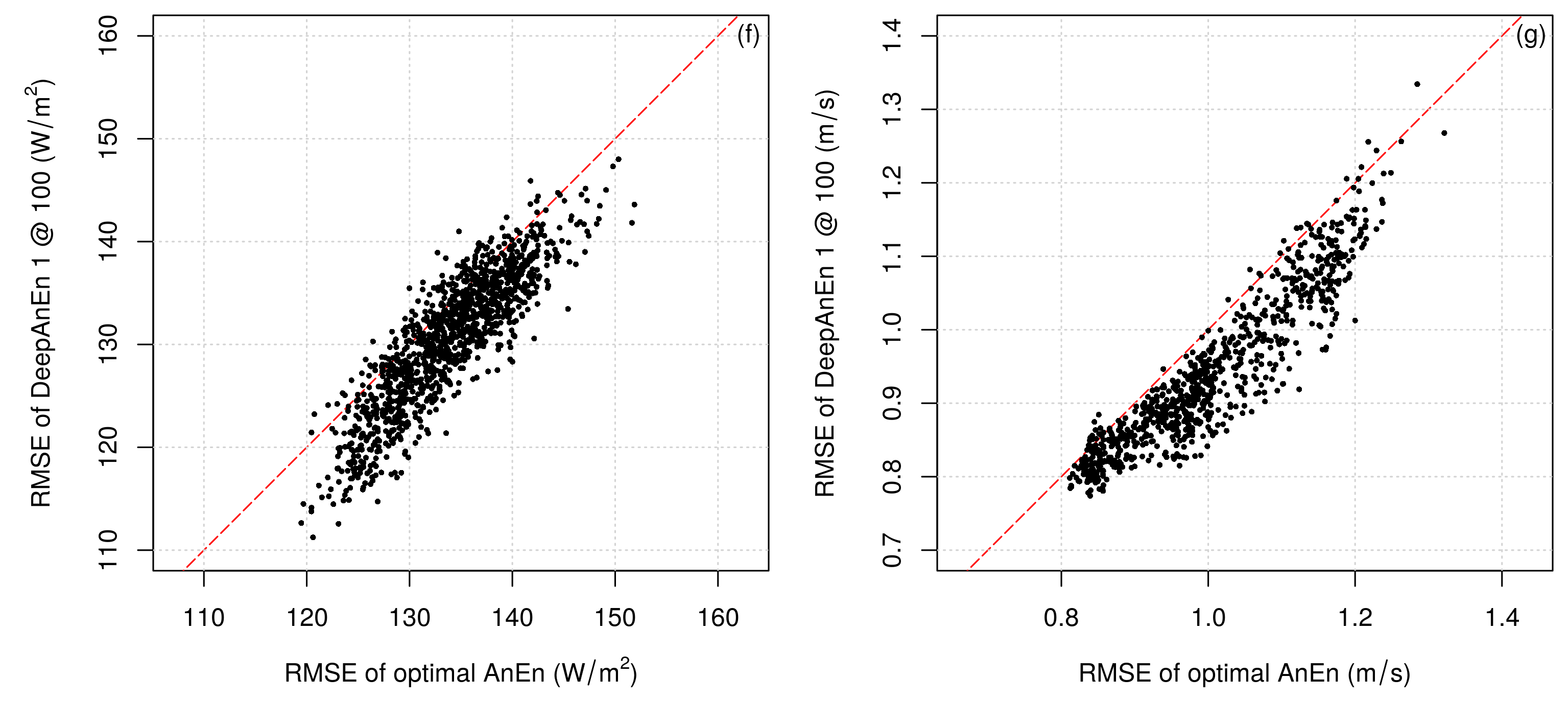
Figure 9: RMSE comparison for spatial predictions between various methods and configurations. (a, d) show the distribution of RMSE and compare the sorted RMSE from each location. (b, c) show the RMSE scatter plots for wind speed forecasts at 80 meters above ground; (e) shows the RMSE scatter plot for solar irradiance forecasts. (f, g) compares the RMSE from the optimal AnEn and DeepAnEn 1 @ 100, for 80-meter wind speed (f) and solar irradiance (g).

To further illustrate the difference among the equally weighted AnEn, the optimal AnEn, and DA, RMSE for solar irradiance and 80-meter wind speed forecasts are compared in Figure 9. Figure 9 (a) shows the sorted RMSE at each location for 80-meter wind speed. RMSE of the equally weighted AnEn is much higher than the RMSE of NAM and DeepAnEn 1 @ 1. In this case, the ML model trained on only one location does not improve DA predictions compared to NAM. However, the optimization of using a trained model shows a great preference compared to the equally weighted AnEn. The ML model, although only trained on one location, is still able to learn the relative importance of 383 forecast variables from NAM and to significantly reduce prediction errors compared to no optimization on weights at all. Going further down is the optimal AnEn and then other two configurations of DA, DeepAnEn 1 @ 100 and DeepAnEn 9 @ 408. The two configurations of DA have similar RMSE, both lower than the optimal AnEn, suggesting DA with the model trained on multiple locations has the ability to outperform the optimal AnEn. Note that training nine individual models would require nine times as much computation as for training one model, given similar amount of training data. However, this additional computation does not necessarily lead to the expected gain in prediction accuracy. Figures 9 (b, c) shows the RMSE scatter plot using the verification results from Figure 9 (a). DeepAnEn 1 @ 1 (in blue) mostly lie on top of the diagonal line, indicating its similarity in RMSE with NAM. The equally weighted AnEn (in yellow) lies high above the diagonal line suggesting the low prediction accuracy. Point clouds of DeepAnEn 1 @ 100, DeepAnEn 9 @ 408, and the optimal AnEn are clustered below the diagonal line, suggesting better accuracy than the baseline NAM predictions.

Figures 9 (d, e) show the RMSE on solar irradiance forecasts following the same argument. Figure 9 (d) shows the sorted RMSE at each location and Figure 9 (e) compares the RMSE scatter plots. There are generally two clusters, one from NAM and the equally weighted AnEn and another one from DeepAnEn 1 @ 1, DeepAnEn 1 @ 100, and the optimal AnEn. In the second cluster, there is a clear cascade in the sorted RMSE that DeepAnEn 1 @ 100 outperforms the optimal AnEn and then the DeepAnEn 1 @ 1. This is supported by the vertical shift of cloud points on Figure 9 (e), from green, purple, to blue. These experiments demonstrate the effectiveness of DA in predicting solar irradiance.

Finally, Figures 9 (f, g) specifically compare RMSE between the best configuration of DA, DeepAnEn 1 @ 100, and the optimal AnEn. In both figures, most of points lie below the diagonal line suggesting DA has a lower RMSE and therefore a higher accuracy in predicting solar irradiance and 80-meter wind speed. Specifically, 85.88% (1034 out of 1204) of the points in Figure 9 (f) and 95.95% (805 out of 839) in Figure 9 (g) lie below the referential line. These results show the ability of DA to predict day time solar irradiance and wind speed variation for a spatial domain, achieving an improved accuracy compared to the optimal AnEn.

5 Discussion and Conclusions

This paper introduces a new technique of generating weather analogs using ML. Specifically, weather analogs are sought in a transformed space generated by a pre-trained ML model, and as a result, the similarity metric is renovated and redefined in the transformed space. We, hereby, highlight some of the major motivation and findings for the ML driven AnEn technique:

1. The conventional similarity metric [1] calculates weighted Euclidean distances in the original predictor variable space. Due to this practice, AnEn is subject to using a few predictor variables and a computationally expensive weight optimization process. DA overcomes the limits on the number of predictors by training an ML model for feature transformation and representation.

2. Optimizing predictor weights for the conventional AnEn is found to be even more difficult for generating spatial predictions or gridded forecast output [15, 54]. However, DA is able to generate more accurate predictions than the optimal AnEn over a spatial domain. This is largely due to the powerful ML model architecture trained using data from multiple sites.

3. Using more weather variables to define weather analogs offers greater flexibility to various weather regimes, and it is more robust to model forecast errors. DA has been found to be more accurate in predicting hard-to-forecast cases compared to AnEn using only a few predictor variables.

4. Finally, DA has also been found to be more tolerant to model updates when increasing the historical archive for weather analog search. During model training using the proposed reverse analog technique, DA builds a relationship between model forecasts and the analysis error, and later on, relies on this relationship to generate informed predictions.

The triplet training architecture is another key to learn effective weather features. Fanfarillo et al. proposed to use a encoder-decoder architecture for analog generation to save computation and memory. They achieve constant scaling in computation and memory when the size of model archive increases. But yet the generative model was not able to achieve as good results as AnEn. This work, however, is able to show that DA outperforms the optimal AnEn with the original similarity metric. This suggests that the features learned by the ML embedding network are more powerful than identifying analogs in the original predictor variable space or in the latent space learned by an auto-encoder. There are two potential reasons: (1) auto-encoder, acting like a data compressor, seeks to represent the complex NWP model forecasts with a few features. The NWP model, however, is highly complex. And there is no guidance when constructing the latent features that will help to generate accurate ensemble forecasts. The only guidance is to represent the NWP model forecasts. The quality of the latent features is yet to be ensured; (2) the features generated by an auto-encoder might not be continuous in the latent space. Clustered points in the latent space might not necessarily correspond to actually similar weather forecasts. Triplet networks, however, were specifically designed to overcome these issues. Its combination with a contrastive loss function particularly encourages to cluster points if they correspond to actual similar features in the original space. These clustered points can then contribute to an ensemble with better quality and improved accuracy (as shown in Figure 5). The reverse analog technique, introduced in Section 2.3, offers specific guidance during the triplet network training, to learn features that would consider the final ensemble prediction and compensate for model errors.

Van den Dool once estimated that $10^{30}$ years are needed to find good analogs. This estimation, fortunately, has been significantly reduced to several years using new analog theories. In general, it was assumed that better analogs can be found given a longer search history and these better analogs can lead to better predictions and improved ensembles. This work, however, shows that with the current implementation of AnEn, the similarity metric is limited in flexibility and model update tolerance. DA offers a good solution to these problems, yet a timely one because of the recent advancement in earth observation, weather modeling, and high-performance computing. Long archives of historical model simulations and observations are becoming easily accessible and DA shows a great capability to harvest the recent advancement in weather analog identification. Future research should be directed to the application of such a framework in extreme weather forecasting and forecasts over a large spatial domain. LSTM is used as the embedding network in this work, but studies are also encouraged to systematically evaluate the performance of different NN s as the embedding network.

References

- Delle Monache et al. [2013] Luca Delle Monache, F. Anthony Eckel, Daran L. Rife, Badrinath Nagarajan, and Keith Searight. Probabilistic Weather Prediction with an Analog Ensemble. Monthly Weather Review, 141(10):3498–3516, October 2013. ISSN 0027-0644, 1520-0493. doi: 10.1175/MWR-D-12-00281.1. URL http://journals.ametsoc.org/doi/10.1175/MWR-D-12-00281.1.
- van den Dool [1989] H. M. van den Dool. A New Look at Weather Forecasting through Analogues. Monthly Weather Review, 117(10):2230–2247, October 1989. ISSN 0027-0644. doi: 10.1175/1520-0493(1989)117¡2230:ANLAWF¿2.0.CO;2. URL https://journals.ametsoc.org/doi/abs/10.1175/1520-0493(1989)117%3C2230%3AANLAWF%3E2.0.CO%3B2. Publisher: American Meteorological Society.
- Toth [1989] Zoltan Toth. Long-Range Weather Forecasting Using an Analog Approach. Journal of Climate, 2(6):594–607, June 1989. ISSN 0894-8755. doi: 10.1175/1520-0442(1989)002¡0594:LRWFUA¿2.0.CO;2. URL https://journals.ametsoc.org/jcli/article/2/6/594/31576/Long-Range-Weather-Forecasting-Using-an-Analog. Publisher: American Meteorological Society.
- Sperati et al. [2017] Simone Sperati, Stefano Alessandrini, and Luca Delle Monache. Gridded probabilistic weather forecasts with an analog ensemble: Gridded Probabilistic Forecasts with an Analog Ensemble. Quarterly Journal of the Royal Meteorological Society, 143(708):2874–2885, October 2017. ISSN 00359009. doi: 10.1002/qj.3137. URL http://doi.wiley.com/10.1002/qj.3137.
- Clemente-Harding [2019] Laura Clemente-Harding. Extension of the Analog Ensemble Technique to the Spatial Domain. PhD thesis, Pennsylvania State University, University Park, Pennsylvania, 2019. URL https://catalog.libraries.psu.edu/catalog/28948273.
- Cervone et al. [2017] Guido Cervone, Laura Clemente-Harding, Stefano Alessandrini, and Luca Delle Monache. Short-term photovoltaic power forecasting using Artificial Neural Networks and an Analog Ensemble. Renewable Energy, 108:274–286, August 2017. ISSN 09601481. doi: 10.1016/j.renene.2017.02.052. URL https://linkinghub.elsevier.com/retrieve/pii/S0960148117301386.
- Hu et al. [2020a] Weiming Hu, Davide Del Vento, and Shiquan Su. Proceedings of the 2020 Improving Scientific Software Conference. Technical report, UCAR/NCAR, June 2020a. URL https://opensky.ucar.edu/islandora/object/technotes:585.
- Alessandrini et al. [2015] S. Alessandrini, L. Delle Monache, S. Sperati, and J. N. Nissen. A novel application of an analog ensemble for short-term wind power forecasting. Renewable Energy, 76:768–781, April 2015. ISSN 0960-1481. doi: 10.1016/j.renene.2014.11.061. URL http://www.sciencedirect.com/science/article/pii/S0960148114007915.
- Zhang et al. [2019] X. Zhang, Y. Li, S. Lu, H. F. Hamann, B. Hodge, and B. Lehman. A Solar Time Based Analog Ensemble Method for Regional Solar Power Forecasting. IEEE Transactions on Sustainable Energy, 10(1):268–279, January 2019. ISSN 1949-3037. doi: 10.1109/TSTE.2018.2832634. Conference Name: IEEE Transactions on Sustainable Energy.
- Wang et al. [2020] Jingyue Wang, Zheng Qian, Jingyi Wang, and Yan Pei. Hour-Ahead Photovoltaic Power Forecasting Using an Analog Plus Neural Network Ensemble Method. Energies, 13(12):3259, January 2020. doi: 10.3390/en13123259. URL https://www.mdpi.com/1996-1073/13/12/3259. Number: 12 Publisher: Multidisciplinary Digital Publishing Institute.
- Candido et al. [2020] Salvatore Candido, Aakanksha Singh, and Luca Delle Monache. Improving wind forecasts in the lower stratosphere by distilling an analog ensemble into a deep neural network. Geophysical Research Letters, 47(15):e2020GL089098, 2020. doi: https://doi.org/10.1029/2020GL089098. URL https://agupubs.onlinelibrary.wiley.com/doi/abs/10.1029/2020GL089098.
- Monache et al. [01 Oct. 2020] Luca Delle Monache, Stefano Alessandrini, Irina Djalalova, James Wilczak, Jason C. Knievel, and R. Kumar. Improving air quality predictions over the united states with an analog ensemble. Weather and Forecasting, 35(5):2145 – 2162, 01 Oct. 2020. doi: 10.1175/WAF-D-19-0148.1. URL https://journals.ametsoc.org/view/journals/wefo/35/5/wafD190148.xml.
- Vanvyve et al. [2015] Emilie Vanvyve, Luca Delle Monache, Andrew J. Monaghan, and James O. Pinto. Wind resource estimates with an analog ensemble approach. Renewable Energy, 74:761–773, February 2015. ISSN 0960-1481. doi: 10.1016/j.renene.2014.08.060. URL http://www.sciencedirect.com/science/article/pii/S0960148114005308.
- Shahriari et al. [2020] M. Shahriari, G. Cervone, L. Clemente-Harding, and L. Delle Monache. Using the analog ensemble method as a proxy measurement for wind power predictability. Renewable Energy, 146:789–801, February 2020. ISSN 0960-1481. doi: 10.1016/j.renene.2019.06.132. URL http://www.sciencedirect.com/science/article/pii/S0960148119309668.
- Junk et al. [2015] Constantin Junk, Luca Delle Monache, Stefano Alessandrini, Guido Cervone, and Lueder von Bremen. Predictor-weighting strategies for probabilistic wind power forecasting with an analog ensemble. Meteorologische Zeitschrift, 24(4):361–379, July 2015. ISSN 0941-2948. doi: 10.1127/metz/2015/0659. URL http://www.schweizerbart.de/papers/metz/detail/24/84737/Predictor_weighting_strategies_for_probabilistic_w?af=crossref.
- Khodayar and Teshnehlab [2015] Mahdi Khodayar and Mohammad Teshnehlab. Robust deep neural network for wind speed prediction. In 2015 4th Iranian Joint Congress on Fuzzy and Intelligent Systems (CFIS), pages 1–5, September 2015. doi: 10.1109/CFIS.2015.7391664.
- Xiaoyun et al. [2016] Qu Xiaoyun, Kang Xiaoning, Zhang Chao, Jiang Shuai, and Ma Xiuda. Short-term prediction of wind power based on deep Long Short-Term Memory. In 2016 IEEE PES Asia-Pacific Power and Energy Engineering Conference (APPEEC), pages 1148–1152, October 2016. doi: 10.1109/APPEEC.2016.7779672.
- Gensler et al. [2016] André Gensler, Janosch Henze, Bernhard Sick, and Nils Raabe. Deep Learning for solar power forecasting — An approach using AutoEncoder and LSTM Neural Networks. In 2016 IEEE International Conference on Systems, Man, and Cybernetics (SMC), pages 002858–002865, October 2016. doi: 10.1109/SMC.2016.7844673.
- Qing and Niu [2018] Xiangyun Qing and Yugang Niu. Hourly day-ahead solar irradiance prediction using weather forecasts by LSTM. Energy, 148:461–468, April 2018. ISSN 0360-5442. doi: 10.1016/j.energy.2018.01.177. URL http://www.sciencedirect.com/science/article/pii/S0360544218302056.
- Frediani et al. [2017] Maria E. B. Frediani, Thomas M. Hopson, Joshua P. Hacker, Emmanouil N. Anagnostou, Luca Delle Monache, and Francois Vandenberghe. Object-Based Analog Forecasts for Surface Wind Speed. Monthly Weather Review, 145(12):5083–5102, December 2017. ISSN 0027-0644, 1520-0493. doi: 10.1175/MWR-D-17-0012.1. URL http://journals.ametsoc.org/doi/10.1175/MWR-D-17-0012.1.
- Delle Monache et al. [2018] Luca Delle Monache, Stefano Alessandrini, Irina Djalalova, James Wilczak, and Jason C. Knievel. Air Quality Predictions with an Analog Ensemble. Atmospheric Chemistry and Physics Discussions, pages 1–36, May 2018. ISSN 1680-7375. doi: 10.5194/acp-2017-1214. URL https://www.atmos-chem-phys-discuss.net/acp-2017-1214/.
- Alessandrini et al. [2018] Stefano Alessandrini, Luca Delle Monache, Christopher M. Rozoff, and William E. Lewis. Probabilistic Prediction of Tropical Cyclone Intensity with an Analog Ensemble. Monthly Weather Review, 146(6):1723–1744, June 2018. ISSN 0027-0644, 1520-0493. doi: 10.1175/MWR-D-17-0314.1. URL http://journals.ametsoc.org/doi/10.1175/MWR-D-17-0314.1.
- Hu and Cervone [2019] Weiming Hu and Guido Cervone. Dynamically Optimized Unstructured Grid (DOUG) for Analog Ensemble of numerical weather predictions using evolutionary algorithms. Computers & Geosciences, 133:104299, December 2019. ISSN 0098-3004. doi: 10.1016/j.cageo.2019.07.003. URL http://www.sciencedirect.com/science/article/pii/S0098300418306678.
- Hu et al. [2020b] Weiming Hu, Guido Cervone, Laura Clemente-Harding, and Martina Calovi. Parallel analog ensemble – the power of weatheranalogs. In Proceedings of the 2020 Improving Scientific Software Conference, May 2020b. doi: 10.5065/p2jj-9878.
- Alessandrini et al. [2019] Stefano Alessandrini, Simone Sperati, and Luca Delle Monache. Improving the Analog Ensemble Wind Speed Forecasts for Rare Events. Monthly Weather Review, 147(7):2677–2692, July 2019. ISSN 0027-0644. doi: 10.1175/MWR-D-19-0006.1. URL https://journals.ametsoc.org/mwr/article/147/7/2677/344570/Improving-the-Analog-Ensemble-Wind-Speed-Forecasts. Publisher: American Meteorological Society.
- Sidel et al. [2020] Alon Sidel, Weiming Hu, Martina Calovi, and Guido Cervone. Heat wave identification using an operational weather model and analog ensemble. In 100th American Meteorological Society Annual Meeting. AMS, 2020.
- Calovi et al. [2018] Martina Calovi, Guido Cervone, Luca Delle Monache, and Weiming Hu. Gfs downscaling using personal weather stations for heat wave vulnerability. AGUFM, 2018:NH31C–0992, 2018.
- Baldi and Chauvin [1993] Pierre Baldi and Yves Chauvin. Neural Networks for Fingerprint Recognition. Neural Computation, 5(3):402–418, May 1993. ISSN 0899-7667. doi: 10.1162/neco.1993.5.3.402. URL https://doi.org/10.1162/neco.1993.5.3.402. Publisher: MIT Press.
- Bromley et al. [1994] Jane Bromley, Isabelle Guyon, Yann LeCun, Eduard Säckinger, and Roopak Shah. Signature Verification using a ”Siamese” Time Delay Neural Network. Advances in neural information processing systems, pages 737–744, 1994.
- Chopra et al. [2005] S. Chopra, R. Hadsell, and Y. LeCun. Learning a similarity metric discriminatively, with application to face verification. In 2005 IEEE Computer Society Conference on Computer Vision and Pattern Recognition (CVPR’05), volume 1, pages 539–546 vol. 1, June 2005. doi: 10.1109/CVPR.2005.202. ISSN: 1063-6919.
- Taigman et al. [2014] Yaniv Taigman, Ming Yang, Marc’Aurelio Ranzato, and Lior Wolf. DeepFace: Closing the Gap to Human-Level Performance in Face Verification. Proceedings of the IEEE conference on computer vision and pattern recognition, pages 1701–1708, 2014. URL https://www.cv-foundation.org/openaccess/content_cvpr_2014/html/Taigman_DeepFace_Closing_the_2014_CVPR_paper.html.
- Hoffer and Ailon [2015] Elad Hoffer and Nir Ailon. Deep Metric Learning Using Triplet Network. In Aasa Feragen, Marcello Pelillo, and Marco Loog, editors, Similarity-Based Pattern Recognition, Lecture Notes in Computer Science, pages 84–92, Cham, 2015. Springer International Publishing. ISBN 978-3-319-24261-3. doi: 10.1007/978-3-319-24261-3˙7.
- Koch [2015] Gregory Koch. Siamese Neural Networks for One-Shot Image Recognition. ICML deep learning workshop, 2:30, 2015.
- Bertinetto et al. [2016] Luca Bertinetto, Jack Valmadre, João F. Henriques, Andrea Vedaldi, and Philip H. S. Torr. Fully-Convolutional Siamese Networks for Object Tracking. arXiv:1606.09549 [cs], September 2016. URL http://arxiv.org/abs/1606.09549. arXiv: 1606.09549.
- Zheng et al. [2017] Zhedong Zheng, Liang Zheng, and Yi Yang. A Discriminatively Learned CNN Embedding for Person Reidentification. ACM Transactions on Multimedia Computing, Communications, and Applications, 14(1):13:1–13:20, December 2017. ISSN 1551-6857. doi: 10.1145/3159171. URL https://doi.org/10.1145/3159171.
- Liu et al. [2019] X. Liu, Y. Zhou, J. Zhao, R. Yao, B. Liu, and Y. Zheng. Siamese Convolutional Neural Networks for Remote Sensing Scene Classification. IEEE Geoscience and Remote Sensing Letters, 16(8):1200–1204, August 2019. ISSN 1558-0571. doi: 10.1109/LGRS.2019.2894399. Conference Name: IEEE Geoscience and Remote Sensing Letters.
- Schroff et al. [2015] Florian Schroff, Dmitry Kalenichenko, and James Philbin. FaceNet: A Unified Embedding for Face Recognition and Clustering. Proceedings of the IEEE conference on computer vision and pattern recognition, pages 815–823, 2015. URL https://www.cv-foundation.org/openaccess/content_cvpr_2015/html/Schroff_FaceNet_A_Unified_2015_CVPR_paper.html.
- Dong and Shen [2018] Xingping Dong and Jianbing Shen. Triplet Loss in Siamese Network for Object Tracking. Proceedings of the European Conference on Computer Vision (ECCV), pages 459–474, 2018. URL https://openaccess.thecvf.com/content_ECCV_2018/html/Xingping_Dong_Triplet_Loss_with_ECCV_2018_paper.html.
- Hochreiter and Schmidhuber [1997] Sepp Hochreiter and Jürgen Schmidhuber. Long Short-Term Memory. Neural Computation, 9(8):1735–1780, November 1997. ISSN 0899-7667. doi: 10.1162/neco.1997.9.8.1735. URL https://doi.org/10.1162/neco.1997.9.8.1735. Publisher: MIT Press.
- Chung et al. [2014] Junyoung Chung, Caglar Gulcehre, KyungHyun Cho, and Yoshua Bengio. Empirical Evaluation of Gated Recurrent Neural Networks on Sequence Modeling. arXiv:1412.3555 [cs], December 2014. URL http://arxiv.org/abs/1412.3555. arXiv: 1412.3555.
- Gao et al. [2019] Mingming Gao, Jianjing Li, Feng Hong, and Dongteng Long. Day-ahead power forecasting in a large-scale photovoltaic plant based on weather classification using LSTM. Energy, 187:115838, November 2019. ISSN 0360-5442. doi: 10.1016/j.energy.2019.07.168. URL http://www.sciencedirect.com/science/article/pii/S0360544219315105.
- Kingma and Ba [2014] Diederik P Kingma and Jimmy Ba. Adam: A method for stochastic optimization. arXiv preprint arXiv:1412.6980, 2014.
- Dyer [2014] Chris Dyer. Notes on noise contrastive estimation and negative sampling. arXiv preprint arXiv:1410.8251, 2014.
- Goldberg and Levy [2014] Yoav Goldberg and Omer Levy. word2vec explained: deriving mikolov et al.’s negative-sampling word-embedding method. arXiv preprint arXiv:1402.3722, 2014.
- Xu et al. [2015] Kun Xu, Yansong Feng, Songfang Huang, and Dongyan Zhao. Semantic relation classification via convolutional neural networks with simple negative sampling. arXiv preprint arXiv:1506.07650, 2015.
- Wang et al. [2018] Peifeng Wang, Shuangyin Li, et al. Incorporating gan for negative sampling in knowledge representation learning. arXiv preprint arXiv:1809.11017, 2018.
- Whitley [1994] Darrell Whitley. A genetic algorithm tutorial. Statistics and computing, 4(2):65–85, 1994.
- Hancock [1994] Peter JB Hancock. An empirical comparison of selection methods in evolutionary algorithms. In AISB workshop on evolutionary computing, pages 80–94. Springer, 1994.
- Vafaie and Imam [1994] Haleh Vafaie and Ibrahim F Imam. Feature selection methods: genetic algorithms vs. greedy-like search. In Proceedings of the international conference on fuzzy and intelligent control systems, volume 51, page 28, 1994.
- Wilt et al. [2010] Christopher Makoto Wilt, Jordan Tyler Thayer, and Wheeler Ruml. A comparison of greedy search algorithms. In third annual symposium on combinatorial search, 2010.
- Augustine et al. [2000] John A Augustine, John J DeLuisi, and Charles N Long. Surfrad–a national surface radiation budget network for atmospheric research. Bulletin of the American Meteorological Society, 81(10):2341–2358, 2000.
- Augustine et al. [2005] John A Augustine, Gary B Hodges, Christopher R Cornwall, Joseph J Michalsky, and Carlos I Medina. An update on surfrad—the gcos surface radiation budget network for the continental united states. Journal of Atmospheric and Oceanic Technology, 22(10):1460–1472, 2005.
- for Environmental Prediction/National Weather Service/NOAA/US Department of Commerce [2015] Environmental Modeling Center/National Centers for Environmental Prediction/National Weather Service/NOAA/US Department of Commerce. Ncep north american mesoscale (nam) 12 km analysis. 2015.
- Clemente-Harding et al. [2016] Laura Clemente-Harding, Guido Cervone, Luca Delle Monache, Sue Ellen Haupt, and Stefano Alessandrini. Analog ensemble (anen): Optimal predictor weighting and exploitation of spatial characteristics in anen generation. AGUFM, 2016:A41G–0131, 2016.
- Fanfarillo et al. [2020] Alessandro Fanfarillo, Behrooz Roozitalab, Weiming Hu, and Guido Cervone. Probabilistic forecasting using deep generative models. GeoInformatica, pages 1–21, 2020.
- Van den Dool [1994] HM Van den Dool. Searching for analogues, how long must we wait? Tellus A, 46(3):314–324, 1994.