Rydberg blockade in an ultracold strontium gas revealed by two-photon excitation dynamics

Abstract

We demonstrate the interaction-induced blockade effect in an ultracold ⁸⁸Sr gas via studying the time dynamics of a two-photon excitation to the triplet Rydberg series $5\mathrm{s}n\mathrm{s}\,^{3}\textrm{S}_{1}$ for five different principle quantum numbers $n$ ranging from 19 to 37. By using a multi-pulse excitation sequence to increase the detection sensitivity we could identify Rydberg-excitation-induced atom losses as low as $<1\%$. Based on an optical Bloch equation formalism, treating the Rydberg-Rydberg interaction on a mean-field level, the van der Waals coefficients are extracted from the observed dynamics, which agree fairly well with ab initio calculations.

I Introduction

The strong Rydberg-Rydberg interactions arising from large electric dipole moments Gallagher2008 are central to the research frontiers using ultracold Rydberg atoms, including quantum information processing with Rydberg-mediated quantum gates Saffman2010 ; Comparat2010 ; Saffman2016 , Rydberg nonlinear optics Pritchard2012a ; Firstenberg2016 , and Rydberg simulators of many-body physics Browaeys2016 ; Browaeys2020 . Recently, there is an increasing interest in extending the studies of Rydberg physics to alkali-earth-like atoms Dunning2016 . Due to the presence of an extra valence electron compared to the well-studied alkalies Gallagher2005 , divalent atoms offer Rydberg series of both singlet and triplet characters with richer interactions in a single element, the possibility of co-trapping Rydberg and ground state atoms Mukherjee2011 ; Wilson2019 ; Madjarov2020 , and the allowance of studying two-electron correlations Kalinski2003 . Alkali-earth-like Rydberg atoms also find applications in realizing spin-squeezing for precision metrology Gil2014 ; Kaubruegger2019 , generating high-fidelity entanglement for quantum information processing Wilson2019 ; Madjarov2020 , as well as simulating strongly correlated many-body systems Mukherjee2011 .

Most applications involving Rydberg atoms rely on the ab initio calculated Rydberg-Rydberg interaction potentials using for example open-source codes Weber2017 ; Robertson2021 , which have been confirmed for alkali atoms by experiments (see like Gallagher2008 ; Marcassa2014 ; Beguin2013 ). Specifically, Ref. Beguin2013 directly extracted the van der Waals (vdW) interaction between two isolated Rydberg atoms by measuring the excitation dynamics and comparing it to solutions of an optical Bloch equation (OBE). The observed suppression of Rydberg excitations at strong interactions is called blockade effect Lukin2001 ; Urban2009 ; Gaetan2009 , which was also studied in larger cold atom ensembles Singer2004 ; Tong2004 ; Heidemann2007 ; Pritchard2010 ; Dudin2012 ; Schauss2012 . Mean-field theories have been applied to account for related observations in bulk atomic gases Tong2004 ; Weimer2008 ; Helmrich2018 ; DeHond2018 .

The ab initio calculations of Rydberg properties in alkali-earth-like systems are much more complicated than that for alkali atoms due to the existing of two-electron effects Vaillant2012 ; Ye2013a ; Vaillant2014 ; Robicheaux2019 . Although the direct method of measuring the vdW interactions like Ref. Beguin2013 provides the most reliable benchmark for these calculations, the experiment requires a challenging setup for being able to control the distance between two isolated single atoms in a large scale ($1\sim 20$ $\mu$m). So far, the experimental studies of the Rydberg-Rydberg interactions in alkali-earth-like atoms are quite limited, where the blockade effect was studied spectroscopically in strontium Zhang2015 ; DeSalvo2016 and high-fidelity entanglement was generated via the strong Rydberg-Rydberg interactions in an optical tweezer experiment Madjarov2020 .

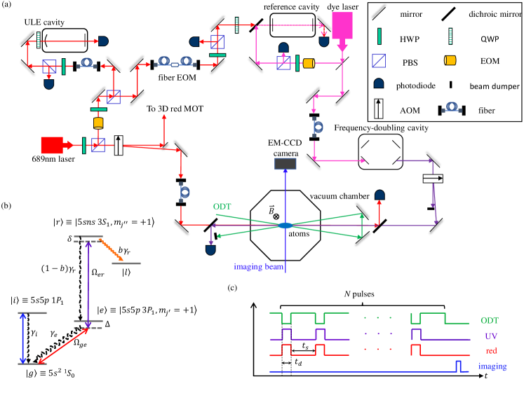
Figure 1: Two-photon pulsed excitation to the $5sns\text{ }^{3}S_{1}$ states. (a) Schematic view of the experimental setup. The abbreviations are: HWP—half wave-plate, QWP—quarter wave-plate, PBS—polarizing beam-splitter, EOM—electro-optic modulator, AOM—accousto-optic modulator, ULE—ultra-low expansion. Many optical elements are omitted here, like lenses. See text for detailed descriptions. (b) The relevant energy levels. The Rydberg state $\ket{r}$ is addressed via a two-photon process from the ground state $\ket{g}$ via an intermediate state $\ket{e}$. $\Omega_{er}$ ($\Omega_{ge}$) represents the Rabi frequency driving the $\ket{e}-\ket{r}$ ($\ket{g}-\ket{e}$) transition and $\Delta$ ($\delta$) is the one-photon (two-photon) detuning. Atoms at $\ket{g}$ are detected by absorption imaging with the broad $\ket{g}-\ket{i}$ transition. $\gamma_{g,e,i}$ are the natural linewidths of the corresponding states and the branching ratio from $\ket{r}$ to $\ket{e}$ ($\ket{l}$) is $1-b$ ($b$). Here $\ket{l}$ represents the low-lying states that $\ket{r}$ decays to, except $\ket{e}$. (c) The $N$-pulse sequence. The two beams are operated simultaneously with $N$ pulses, each of equal duration $t_{d}$ and equally separated by $t_{s}$. The ODT is temporarily switched off during the excitation pules.

In this work we present a systematic study of the Rydberg blockade effect in an ultracold gas of ⁸⁸Sr atoms using two-photon excitations from the ground state $5s^{2}\text{ }^{1}S_{0}$ ($\equiv\ket{g}$) to the triplet Rydberg series $5sns\text{ }^{3}S_{1}$ ($\equiv\ket{r}$) via the long-lived $5s5p\text{ }^{3}P_{1}$ state ($\equiv\ket{e}$), where five different principle quantum numbers $n$ in the range of $19\leq n\leq 37$ are addressed. By making use of a multi-pulse scheme to increase the detection sensitivity DeSalvo2016 , we could identify Rydberg-excitation-induced atom losses smaller than $1\%$. The suppression of the Rydberg excitations is observed by comparing the dynamics at two different atomic densities. The measurements are modelled by a single-particle OBE taking the Rydberg-Rydberg interaction into account with a self-consistent mean-field theory Helmrich2018 ; DeHond2018 , from which the vdW interaction coefficients $C_{6}$ are extracted and compared to the ab initio calculations in Ref. Vaillant2012 . Despite the simplicity of our model, a fairly good agreement is found between the measured and calculated $C_{6}$ coefficients.

The article is organized as follows: The experimental details are presented in Sec. II.1 and the mean-field model is introduced in Sec. II.2. The experimental results and the mean-field modelling are discussed in Secs. III.1 and III.2, from which the vdW coefficients are extracted and compared to theoretical calculations in Sec. III.3. We conclude the paper with Sec. IV.

II Methods

II.1 Experimental Setup

Our experimental setup for producing ultracold strontium gases via a two-stage magneto-optical cooling and trapping has been described previously in Refs. Nosske2017 ; Hu2019 ; Qiao2019a . In brief, a three-dimension (3D) magneto-optical trap (MOT) operating on the broad $\ket{g}\rightarrow 5s5p\text{ }^{1}P_{1}$ ($\equiv\ket{i}$) transition at $461\text{\,}\mathrm{n}\mathrm{m}$ is loaded from a two-dimension (2D) MOT using the same transition Nosske2017 . Atoms in this broadband MOT can decay to the $5s5p\text{ }^{3}P_{2}$ state, which is long-lived and magnetically trappable Nagel2003 . Then, via a single-frequency repumping at $481\text{\,}\mathrm{n}\mathrm{m}$ Hu2019 , atoms accumulated in the MOT magnetic quadrupole field for $5\text{\,}\mathrm{s}$ are transferred to a second 3D MOT (red MOT) operating on the narrow $\ket{g}\rightarrow\ket{e}$ transition with a natural linewidth of $\gamma_{e}=2\pi\times$ $7.5\text{\,}\mathrm{k}\mathrm{H}\mathrm{z}$. The red MOT stage lasts for about $200\text{\,}\mathrm{m}\mathrm{s}$ Qiao2019a and a crossed optical dipole trap (ODT) at $532\text{\,}\mathrm{n}\mathrm{m}$ is turned on $150\text{\,}\mathrm{m}\mathrm{s}$ before switching off the red MOT. Then the atoms are held in the ODT for certain time before applying Rydberg excitation pulses. The two ODTs cross at an angle of $18\text{\,}\mathrm{\SIUnitSymbolDegree}$ [see Fig. 1(a)], which results in an elongated atomic cloud with an aspect ratio of about $3:1$ ($\sim$$25\text{\,}\mu\mathrm{m}$ in the radial direction). Due to the very small collisional rates in the gas of ground state ⁸⁸Sr atoms Yan2011 , the atomic density monotonically decays during the holding in the ODT while the temperature and cloud size remain almost unchanged. The resulting atomic densities are listed in Table 1 at holding times of $100\text{\,}\mathrm{m}\mathrm{s}$ and $1000\text{\,}\mathrm{m}\mathrm{s}$ for various principle quantum numbers.

The Rydberg states $\ket{r}$ are addressed via a two-photon process [see Fig. 1(b) for the corresponding level structures]. The optical setup for generating and controlling the two excitation beams is schematically shown in Fig. 1(a). The 689-nm red beam driving the $\ket{g}-\ket{e}$ transition is delivered from an external cavity diode laser, which is frequency locked to a passive ultra-stable cavity resulting in a linewidth smaller than $10\text{\,}\mathrm{k}\mathrm{H}\mathrm{z}$ Qiao2019a . The upper transition ($\ket{e}-\ket{r}$) is driven by a UV beam at $\sim$$319\text{\,}\mathrm{n}\mathrm{m}$, which is obtained by frequency doubling a dye laser using resonant cavity second harmonic generation Arias2017 . The commercial dye laser (Matisse 2 DX, Sirah) is locked to a low-finesse ($\sim 700$) reference cavity to reduce the linewidth (below $20\text{\,}\mathrm{k}\mathrm{H}\mathrm{z}$ over $1\text{\,}\mathrm{m}\mathrm{s}$ Couturier2018 ). Via a standard PDH setup, the length of this low-finesse cavity is stabilized to the frequency-locked 689-nm laser, between which a fiber electro-optic modulator (EOM) is inserted. Since one of the first-order modulation sidebands is used in the stabilization, output frequency of the dye laser can be tuned by the EOM driving frequency to cover the free spectral range of the reference cavity ($\sim$$1.2\text{\,}\mathrm{G}\mathrm{H}\mathrm{z}$). The power of both excitation beams are actively stabilized before the last AOMs for switching and monitored after passing through the atomic cloud with two photodiodes [see Fig. 1(a)].

The two excitation beams counter-propagate horizontally along the axial direction of the atomic cloud [see Fig. 1(a)]. The red (UV) beam is linearly polarized in the horizontal (vertical) direction with a $1/e^{2}$-diameter of $1.4\text{\,}\mathrm{m}\mathrm{m}$ ($1.2\text{\,}\mathrm{m}\mathrm{m}$). A quantization field of about $1.16\text{\,}\mathrm{G}$ is applied vertically, giving rise to a Zeeman splitting of about $h\times$$4.86\text{\,}\mathrm{M}\mathrm{H}\mathrm{z}$ ($8.10\text{\,}\mathrm{M}\mathrm{H}\mathrm{z}$) for the $\ket{e}$ ($\ket{r}$) state. The frequency of the 689-nm light is tuned close to the $\sigma^{+}$ transition ($\Delta m_{j}=+1$) such that $\ket{e}$ refers to the $m_{j^{\prime}}=+1$ level of the $5s5p\text{ }^{3}P_{1}$ state hereafter. Here $m_{j}$ are the magnetic quantum numbers. The vertically polarized UV beam drives only the $\pi$ transition ($\Delta m_{j}=0$), $\ket{r}$ also refers to the $m_{j^{\prime\prime}}=+1$ level of Rydberg states. As seen in Fig. 1(b), the one-photon (two-photon) detuning is defined as $\Delta=\omega_{\textrm{red}}-(\omega_{e}-\omega_{g})$ [$\delta=\omega_{\textrm{UV}}+\omega_{\textrm{red}}-(\omega_{r}-\omega_{g})$], where $\omega_{\textrm{red}}$ ($\omega_{\textrm{UV}}$) is the angular frequency of the red (UV) excitation light and $\hbar\omega_{g,e,r}$ are the energies of corresponding levels. A loss state $\ket{l}$ is introduced to represent all the lower-lying states, that the Rydberg state $\ket{r}$ decays to, except $\ket{e}$. The branching ratio $b$ from $\ket{r}$ into $\ket{l}$ can be calculated to be $2/3$ using the Wigner-Eckart theorem DeSalvo2016 .

The excitation sequence is schematically illustrated in Fig. 1(c). The two excitation beams are pulsed with $N$ equally spaced (of $t_{s}$) pulses of a duration $t_{d}$. To avoid the possible differential AC Stark effects on both red and UV transitions, the ODT is also pulsed simultaneously with the excitation beams. We keep $t_{s}$ long enough when compared to the lifetimes of $\ket{r}$ and $\ket{e}$, such that all the atoms populate $\ket{g}$ at the beginning of each pulse. The remaining ground state atom number after the pulse sequence is recorded by absorption imaging on the broad $\ket{g}\rightarrow\ket{i}$ transition.

II.2 The mean-field model

Describing the Rydberg-Rydberg interaction on a mean-field level, the evolution of the system within a single excitation pulse can be modelled by a single-particle OBE with dephasing effects in the Lindblad form ($\hbar=1$) DeSalvo2016 ; Helmrich2018 ; DeHond2018

$$\dot{\rho}=-i[H,\rho]+\sum\limits_{i}L_{i}\rho L_{i}^{\dagger}-\frac{1}{2}\{L_{i}^{\dagger}L_{i},\rho\}\,.$$ (1)

Here $\rho$ is the density matrix for a four-level system of $\ket{g}$, $\ket{e}$, $\ket{r}$, and $\ket{l}$ (see Fig. 1(b)), and $[\cdots]$ ($\{\cdots\}$) denotes the (anti-)commutator. We refer to the matrix element of $\rho$ as $\rho_{ab}\ket{a}\bra{b}$ with $a,b\in\{g,e,r,l\}$. In the experiment, we monitor the remaining atom number fraction in the ground state $\ket{g}$ after the excitation, which can be represented as

$$1-p_{d}=1-\rho_{ll}-b\rho_{rr}.$$ (2)

Here $p_{d}$ is the loss fraction of a pulse of length $t_{d}$, including all the atoms populated the loss state $\ket{l}$ during and after the single-pulse excitation.

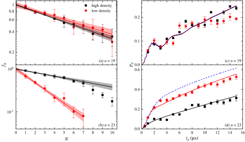
Figure 2: Measurements of the loss fraction per pulse $p_{d}$ for $n=19$ and $n=23$. (a, b) The remaining fraction of atoms $f_{N}$ as a function of the pulse number $N$ for these two states at two different atomic densities (see Table 1). The solid curves are fits to Eq. (5) to extract $p_{d}$ and the shaded areas mark the $95\%$ confidence level. See text for detailed discussions. (c, d) $p_{d}$ as a function of the single-pulse length $t_{d}$. In (c), the black, red, and blue curves are parameter-free calculations for the $n=19$ state with $V/h=0.62$, 0.10, and 0 (see text), respectively. In (d), the solid curves are fits of the high- and low-density data to the mean-field model, from which we obtain $\gamma_{er}/2\pi=$ $0.98(36)\text{\,}\mathrm{M}\mathrm{H}\mathrm{z}$, $V^{e}/2\pi=$ $-71(10)\text{\,}\mathrm{M}\mathrm{H}\mathrm{z}$ for the high-density measurement (black curve), and $\gamma_{er}/2\pi=$ $0.10(9)\text{\,}\mathrm{M}\mathrm{H}\mathrm{z}$, $V^{e}/2\pi=$ $-3.4(7)\text{\,}\mathrm{M}\mathrm{H}\mathrm{z}$ for the low-density data (red curve). The fitted parameters are listed in Table 1. As a comparison, the blue dashed line represents the non-interacting case ($V=0$) with $\gamma_{er}/2\pi=$ $0.10\text{\,}\mathrm{M}\mathrm{H}\mathrm{z}$.

The Hamiltonian $H$ governing the two-photon excitation dynamics Helmrich2018 ; DeHond2018 reads

$$H= (\frac{\Omega_{ge}}{2}\ket{g}\bra{e}+\frac{\Omega_{er}}{2}\ket{e}\bra{r}+h.c.)$$ (3)

$$-(\delta-V\rho_{rr}^{2})\ket{r}\bra{r}-\Delta\ket{e}\bra{e}\,,$$

where the Rabi frequencies and detunings are as shown in Fig. 1(b) and $\rho_{rr}$ is the Rydberg fraction. We have omitted the diagonal term with $\ket{l}$ since it plays no role in determining the population dynamics. The characteristic interaction energy $V$ reads

$$V=C_{6}(\frac{4\pi}{3}n_{0})^{2}\,.$$ (4)

Here $C_{6}$ is the coefficient for the vdW interaction between atoms in $\ket{r}$ and $n_{0}$ is the ground state atomic density. This mean-field form is derived self-consistently in Ref. Helmrich2018 .

The spontaneous decays of $\ket{e}$ and $\ket{r}$ are described by quantum jump operators $L_{e}=\sqrt{\gamma_{e}}\ket{g}\bra{e}$ and $L_{r}=\sqrt{(1-b)\gamma_{r}}\ket{e}\bra{r}+\sqrt{b\gamma_{r}}\ket{l}\bra{r}$, where $b=2/3$ is the branching ratio from $\ket{r}$ to $\ket{l}$ Footnote1 . Effects like laser frequency noises, magnetic field fluctuations, and Doppler effects, cause the fluctuations of the detunings and lead to dephasing, especially the two-photon detuning $\delta$, can be accounted for by additional jump operators in the form of $L_{er}=\sqrt{\gamma_{er}}\ket{r}\bra{r}$ and $L_{ge}=\sqrt{\gamma_{ge}}\ket{e}\bra{e}$. $\gamma_{ge}$ is characterized by measuring the damped Rabi oscillations between $\ket{g}$ and $\ket{e}$ (see Appendix A).

III Results

III.1 The noninteracting case

Table 1: Rydberg-Rydberg interaction. $n_{0}$ are the atomic densities with determination uncertainties in the corresponding brackets. Two free parameters, the mean-field interaction energy $V^{e}=C_{6}^{e}(\frac{4\pi}{3}n_{0})^{2}$ and the dephasing rate $\gamma_{er}$, are extracted from experiments and listed (see text for details). The numbers in brackets are the fitting errors from the measurement statistics, while those in super- and sub-scripts are systematic uncertainties resulting from the Rydberg lifetime ($1/\gamma_{r}$) uncertainty Kunze1993 .

$n$	$n_{0}$	$V^{e}/h$	$\gamma_{er}/2\pi$	Rydberg lifetime ($1/\gamma_{r}$) Kunze1993
	$10^{12}$ cm-3	MHz	MHz	$\mu$s
$19$	1.47(21)	$0^{+4.2}$	0.03(1)	$1.83\pm 0.20$
	0.58(13)
$23$	1.14(19)	$71(10)^{+31}_{-18}$	$0.98(36)^{+0.06}_{-0.08}$	$3.36\pm 0.71$
	0.40(7)	$3.4(7)^{+1.9}_{-1.1}$	$0.10(9)^{+0.01}_{-0.03}$
$27$	1.52(25)	$226(18)^{+63}_{-37}$	$0.70(9)^{+0.06}_{-0.27}$	$5.9\pm 1.2$
	0.62(9)	$48(4)^{+21}_{-12}$	$0.31(9)^{+0.02}_{-0.03}$
$30$	0.88(25)	$689(94)^{+174}_{-101}$	$1.13(31)^{+0.02}_{-0.05}$	$8.4\pm 1.8$
	0.33(10)	$31(14)^{+17}_{-13}$	$1.31(12)^{+0.04}_{-0.07}$
$37$	$0.95(11)$	$2870(194)^{+446}_{-240}$	$2.41(37)^{+0.19}_{-0.30}$	$16.9\pm 3.6$
	0.36(4)	$321(31)^{+61}_{-38}$	$1.47(16)^{+0.07}_{-0.10}$

Figure 2(a) shows the measurement of the fractional ground state atom number $f_{N}$ as a function of the applied pulse number $N$ with $t_{d}=$ $4\text{\,}\mu\mathrm{s}$ and $t_{s}=$ $50\text{\,}\mu\mathrm{s}$ [see Sec. II.1 and Fig. 1(c)] at two different atomic densities for $n=19$ (see Table 1). The Rabi frequencies $\Omega_{ge}$ and $\Omega_{er}$ are calibrated to be $2\pi\times$ $813(20)\text{\,}\mathrm{k}\mathrm{H}\mathrm{z}$ and $2\pi\times$ $862(40)\text{\,}\mathrm{k}\mathrm{H}\mathrm{z}$ by driving Rabi oscillations between $\ket{g}$ and $\ket{e}$ state and measuring the Aulter-Townes splitting (ATS) of $\ket{e}$ caused by the UV light, respectively. The details of these calibrations are presented in the Appendix A. The one-photon (two-photon) detuning $\Delta$ ($\delta$) is $2\pi\times$$3\text{\,}\mathrm{M}\mathrm{H}\mathrm{z}$ ($2\pi\times$$0.27\text{\,}\mathrm{M}\mathrm{H}\mathrm{z}$).

Since $t_{s}$ is long compared to the lifetimes of both $\ket{r}$ $\{1/\gamma_{r}=$1.83(20)\text{\,}\mu\mathrm{s}$$ Kunze1993 $\}$ and $\ket{e}$ ($1/\gamma_{e}\sim$$21\text{\,}\mu\mathrm{s}$), we can safely assume that all the atoms are at the ground state at the beginning of each pulse. The fraction of lost atoms $p_{d}$ due to a single pulse is a constant if the interaction $V$ is unchanged or zero during the measurement and the remaining atom fraction $f_{N}$ as a function of $N$ is expressed as

$$f_{N}=(1-p_{d})^{N},$$ (5)

which is used to fit the experiment data in Figs. 2(a) and (b) to extract the corresponding loss fraction per excitation pulse $p_{d}$. In Fig. 2(c) we show the measurement of $p_{d}$ with different pulse lengths $t_{d}$. Similar $p_{d}$ are observed for all the data points at two densities differed by a factor of about 2.5 (see Table 1). Eq. (1) is numerically solved with and without including the vdW interactions to obtain $p_{d}$ from Eq. (2), which are also shown in Fig. 2(c). Here in the numerical calculations the dephasing term $\gamma_{ge}$ is determined experimentally (see Appendix A), $\gamma_{er}$ is set to zero, and the $C_{6}$ coefficient is from Ref. Vaillant2012 . By comparing the experimental measurements and the numerical results we conclude that the vdW interactions are negligible for the observed excitation dynamics at $n=19$. However, an upper bound of the interaction $V$ can still be obtained, as will be discussed later in Sec. III.2 and also shown in Table 1.

III.2 The interacting case

An example measurement of $f_{N}$ for the $n=23$ state with $t_{d}=$ $4\text{\,}\mu\mathrm{s}$ and $t_{s}=$ $50\text{\,}\mu\mathrm{s}$, similar as that for $n=19$ in Fig. 2(a), is shown in Fig. 2(b). The Rabi frequencies $\Omega_{ge}$ and $\Omega_{er}$ are $2\pi\times$ $784(5)\text{\,}\mathrm{k}\mathrm{H}\mathrm{z}$ and $2\pi\times$ $1225(7)\text{\,}\mathrm{k}\mathrm{H}\mathrm{z}$, respectively, and $\Delta$ ($\delta$) is $2\pi\times$$3\text{\,}\mathrm{M}\mathrm{H}\mathrm{z}$ ($-2\pi\times$$0.09\text{\,}\mathrm{M}\mathrm{H}\mathrm{z}$). We fit the experimental data in 2(b) to Eq. (5). At the low density all the measured points fit very well to the equation, while at the high density only data up to $N=5$ is used in the fitting due to the non-negligible change of $V$ after significant decreasing of atomic densities due to atom losses. The measurements at larger $N$ showing heavier losses agree with the fact that Rydberg excitations are less suppressed at smaller atomic densities.

Similar measurements of $p_{d}$ for $n=23$ as those in Fig. 2(c) are also performed and presented in Fig. 2(d). We observe a much smaller $p_{d}$ at the higher atomic density, especially with longer pulses. To extract quantitative information about the vdW interactions, we fit the data in Figs. 2(c) and 2(d) to numerical solutions of Eq. (1), the implementation of which is benchmarked with previous measurements in Refs. DeSalvo2016 ; DeHond2018 (see Appendix B). The fit is done by minimizing the following cost function

$$\chi=\sum\limits_{i}[p_{d}^{t}(t_{i})-y_{i}]^{2}/\sigma_{i}^{2},$$ (6)

where $y$ and $\sigma$ are the measured $p_{d}$ and their corresponding uncertainties [see Figs. 2(c) and 2(d)]. The theoretical loss fraction per pulse $p_{d}^{t}$ is obtained from Eq. (2) by numerically solving Eq. (1) for certain pulse length $t_{d}$. For each $n$ and each density, the interaction parameter $V$ and the dephasing rate $\gamma_{er}$ are the two fitting parameters, while others are either experimentally determined or from existing literatures (see Appendix A). As seen in Fig. 2(d), the experimental data can be fitted well by the mean-field model (solid curves) with the obtained fitting parameters ($V^{e}$ and $\gamma_{er}$) listed in Table 1. The numbers in brackets indicate the fitting errors coming from the error bars shown in Fig. 2(d).

In the above fitting procedure, the dominating systematic uncertainties (indicated by super- and sub-scripts for the fitting parameters in Table 1) are from the Rydberg-state lifetimes $1/\gamma_{r}$, which are taken or scaled from Ref. Kunze1993 . For $n=19$ and $23$ the lifetimes measured there are directly used, while for higher $n$ they are scaled from the lifetime of $n=23$ by assuming $\gamma_{r}\propto(n-\delta n)^{-3}$ with the quantum defects $\delta n$ from Ref. Couturier2019 . Here we only take the radiative lifetimes into consideration since the blackbody-radiation-induced transitions to neighbouring levels may still contribute to the blockade effect. We are aware of the lifetime measurement of $n=35$ in Ref. Kunze1993 and $n=38$ in Ref. Camargo2016 and the scaled lifetime of $n=37$ in Table 1 agrees better with the latter.

In total, the same measurements as those presented in Fig. 2 are performed for five different principle quantum numbers of $n=19,23,27,30,37$. The data is fitted to the mean-field model in Sec. II.2 following the procedure outlined above and all the fitted parameters are listed in Table 1. For the $n=19$ state, an upper bound of the interaction energy $V^{e}$ is given instead of a fitted value. Larger interaction energies $V^{e}$ are obtained for higher densities and larger $n$. In most cases, the dephasing rate $\gamma_{er}$ is larger when the interaction is stronger, indicating a interaction-induced dephasing DeSalvo2016 .

III.3 The vdW coefficients

Figure 3: The vdW coefficients $C_{6}$. The black and red points are from fits to the experimental data at high and low densities, respectively, while the blue ones are from Ref. Vaillant2012 . See text for more details.

Via the relation in Eq. (4), we extract the vdW coefficients $C_{6}$ for the measured principle quantum numbers $n$ from the fitted characteristic interaction energy $V^{e}$ and compare them in Fig. 3 to the values calculated in Ref. Vaillant2012 (blue points). For each $n$ (except $n=19$), two $C_{6}$ values are obtained from the high- (black circles) and low-density (red circles) measurements, respectively. The error bars represent the uncertainties coming from the errors in fitting $V^{e}$ and determining the atomic densities, both of which are indicated as numbers in brackets in Table 1. The shaded areas mark the uncertainties of $C_{6}$ resulting from the systematic errors of $V^{e}$ when performing the fits (see Table 1 and Sec. III.2).

The dependence of fitted $C_{6}$ values on $n$ agree qualitatively with the theoretical calculations based on the single-active-electron (SAE) approximation Vaillant2012 , which is appropriate for high-$n$ states ($n\geq 30$ in Ref. Vaillant2012 ). The blue points in Fig. 3 for the three $n<30$ states are direct extrapolations of the calculation. The largest deviations between experimental and theoretical values happen at $n=23$ and $n=37$. For $n=23$, the fitted $C_{6}$ from the high-density (low-density) data is a factor of 4 (2) larger than the extrapolated value, which may be due to the inaccuracy of the SAE model for lower-$n$ states. For $n=37$, the measured $C_{6}$ is smaller than the SAE calculation by a factor of 3. This may be caused by the neglect of effects like level crossings with other molecular potentials and the higher-order terms in the multipole expansion using the current mean-field model, which play more important roles with stronger interactions at higher $n$.

However, we also note that larger uncertainties of the measured $C_{6}$ could be possible due to imperfections of the experiments as well as possibly larger uncertainties of Rydberg lifetime determination. For example, we have checked laser frequency drifts in our modelling (not included in Fig. 3), especially that of the UV laser affecting the two-photon detuning $\delta$. A drift of $2\pi\times$ $100\text{\,}\mathrm{k}\mathrm{H}\mathrm{z}$ in $\delta$ would lead to a change of about $15\%$ in the fitted $V$ for the $n=23$ high-density measurement (see Table 1). This effect is more significant when the drifting is not small compared to the interaction energy, i.e. the low-density measurements at smaller $n$. We also cannot rule out the effect of any possible residual DC electric fields in our setup, which can lead to smaller $C_{6}$ values Ravets2015 . The used Rydberg lifetimes in our model are scaled from Ref. Kunze1993 and even larger uncertainties could happen. As mentioned in the second last paragraph of Sec. III.2, disagreements are observed among the scaled $n=37$ lifetime in Table 1, the $n=35$ measured in Ref. Kunze1993 , and that for $n=38$ in Ref. Camargo2016 . Significant improvements could be obtained by having better control on the experimental parameters and performing more precise calculations or measurements on the Rydberg lifetimes.

IV Conclusion

In conclusion, we have shown the blockade effect in two-photon excitations of strontium triplet Rydberg states by directly measuring the density-dependent excitation dynamics. Using a mean-field model we have extracted the vdW interaction coefficients $C_{6}$ from the measured dynamics and compared the results to theoretical calculations. Considering the simplicity of our model, the agreement between the extracted and calculated $C_{6}$ values is fairly good. Such a method could be the first option to investigate the Rydberg physics, when the Rydberg-Rydberg interaction potentials are not well-known for the studied atomic species and no advanced experimental setup like optical tweezers Beguin2013 is available. However, improvements from both the experimental and theoretical sides are needed to mitigate the still existing experiment-theory deviations.

Appendix A Calibrations of experimental parameters

A.1 Rabi oscillations between $\ket{g}$ and $\ket{e}$

The Rabi frequency $\Omega_{ge}$ is calibrated by directly monitoring the Rabi oscillation between $\ket{g}$ and $\ket{e}$ states. The resonance position of $\ket{g}-\ket{e}$ transition is characterized by performing absorption imaging using this narrow line, the details of which can be found elsewhere Hu2021 . For driving the Rabi oscillation, we start from atoms at the ground state in the ODT and apply an on-resonance pulse with the power used in the Rydberg excitation, after which the ground state atom number is measured via absorption imaging on the $\ket{g}-\ket{i}$ transition within $1\text{\,}\mu\mathrm{s}$. This imaging time is short compared to the $\ket{e}$ lifetime ($\sim$ $21\text{\,}\mu\mathrm{s}$), thus minimizing the decay from $\ket{e}$ to $\ket{g}$ during the detection.

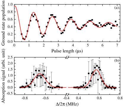
Figure 4: Calibrations of Rabi frequencies. (a) Rabi oscillation between $\ket{g}$ and $\ket{e}$. The solid lines are fits to a damped cosinusoidal function (see text) and the obtained fitting parameters are: $\Omega_{ge}/2\pi=$ $784(5)\text{\,}\mathrm{k}\mathrm{H}\mathrm{z}$, $\tau=$ $3.0(3)\text{\,}\mu\mathrm{s}$, and $t_{0}=$ $0.05(2)\text{\,}\mu\mathrm{s}$. (b) ATS caused by the UV light measured via absorption imaging on the red transition. The data is fitted to the analytic expression in Eq. (7), from which we obtain: $\Omega_{er}/2\pi=$ $1235(13)\text{\,}\mathrm{k}\mathrm{H}\mathrm{z}$ and the UV detuning $\delta_{er}/2\pi=$ $86(7)\text{\,}\mathrm{k}\mathrm{H}\mathrm{z}$.

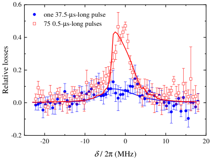
Figure 5: Comparison between the experimental data (blue and red points) from Fig. 1(b) of Ref. DeHond2018 and our mean-field calculation (solid curves). See text for descriptions.

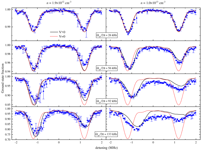
Figure 6: Comparison between the experimental data from Figs. 8 and 9 of Ref. DeSalvo2016 and our mean-field calculation. The black curves represent the case of including the Rydberg interaction term while the red dashed ones are free of interaction ($V=0$). See text for more details.

One example of the Rabi oscillation is shown in Fig. 4(a). The data is fitted to a damped cosinusoidal function $A\exp[-(t-t_{0})/\tau]\cos[\Omega(t-t_{0})]+y_{0}$ to extract the oscillation frequency $\Omega$ and the decay time constant $\tau$. We introduce $t_{0}$ in the fits to account for the finite rising and falling edges of the square pulses used in the experiment ($\sim$$50\text{\,}\mathrm{n}\mathrm{s}$ for both). The detection fidelity is inferred to be about $96\%$.

The oscillation frequency $\Omega$ is interpreted as the Rabi frequency $\Omega_{ge}$ and the decay time constant is related to the dephasing term $\gamma_{ge}$ as $\gamma_{ge}=2/\tau-\gamma_{e}$ in the limit of $1/\tau\gg\gamma_{e}$. However, we observed a much smaller decay rate of the Rabi oscillations for smaller Rabi frequencies ($\sim$$20\text{\,}\mu\mathrm{s}$). Such a dependence of $\tau$ on the Rabi frequency suggests homogeneous dephasing effects and may result from the characteristic phase noise distribution of our PDH-locked laser Qiao2019a , where only noises at frequencies around $\Omega_{ge}$ play the important role for the dephasing. The inhomogeneous Doppler shifts due to the finite temperature (with a Doppler width $\sim 2\pi\times$ $52\text{\,}\mathrm{k}\mathrm{H}\mathrm{z}$) have significant effects only when the power-broadened linewidth is around the Doppler one.

A.2 The UV-induced Aulter-Townes splitting

To characterize the Rabi frequency $\Omega_{er}$ and the two-photon detuning $\delta$, we measure the ATS of the $\ket{e}$ state via probing the absorption of a weak red beam by the atomic cloud in the presence of a strong UV light. The red probe light is overlapped with our blue imaging beam and we use a standard sequence for performing the red absorption imaging with a pulse of $150\text{\,}\mu\mathrm{s}$ Hu2021 . The total absorption over the whole atomic cloud is measured as a function of the probe detuning, as shown in Fig. 4(b) for $n=23$.

The spectrum is fitted to an analytic expression for the ATS [solid line in Fig. 4(b)] Fleischhauer2005 , which reads

$$\sigma\propto\frac{\gamma_{ge}^{2}\gamma_{er}+\gamma_{er}\delta^{2}+\gamma_{ge}\Omega_{er}^{2}/4}{(\gamma_{er}\delta+\gamma_{ge}\Delta)^{2}+(\gamma_{er}\gamma_{ge}-\delta\Delta+\Omega_{er}^{2}/4)^{2}}\,.$$ (7)

Here $\sigma$ represents the absorption cross section. The UV Rabi frequency $\Omega_{er}$ and the two-photon detuning $\delta$ is obtained from this fitting. The two dephasing terms $\gamma_{ge}$ and $\gamma_{er}$ are also free fitting parameters. In Fig. 4(b), $\gamma_{ge}=2\pi\times 0.08(2)$ is smaller than the dephasing rate obtained in Fig. 4(a) due to smaller $\Omega_{ge}$ used here. We obtain $\gamma_{er}=2\pi\times 0.04(2)$, which agrees with the fitted dephasing in Table 1 for the low-density data.

Appendix B Benchmarking the mean-field model

The mean-field model presented in Sec. II.2 is benchmarked here with previously published experimental data from two different experiments, e.g. Refs. DeHond2018 and DeSalvo2016 .

The authors in in Ref. DeHond2018 used the same treatment of the Rydberg-Rydberg interaction term as presented here and they simplified the four-level system to a three-level problem by adiabatically elimilating the intermediate level $\ket{e}$ due to a large one-photon detuning ($\sim 2\pi\times$$100\text{\,}\mathrm{M}\mathrm{H}\mathrm{z}$). The experimental data in Fig. 1(b) of Ref. DeHond2018 is reproduced in Fig. 5, where the atomic losses were measured as a function of the two-photon detuning $\delta$ for two different excitation cases, e.g. a single long excitation pulse of $37.5\text{\,}\mu\mathrm{s}$ (red squares) and 75 equally-separated short pulses of $0.5\text{\,}\mu\mathrm{s}$ (blue circles). The latter pulse scheme is similar as what we implement here [see Fig. 1(c)]. Two theoretical curves modelling these two excitation schemes with parameters taken from Ref. DeHond2018 are also shown in Fig. 5, which agree quite well with the experimental data.

The comparison between our mean-field calculations with the experimental data shown in Figs. 8 and 9 of Ref. DeSalvo2016 is presented in Fig. 6, where atom losses in an optically trapped strontium gas were recorded in the same multi-pulse excitation scheme as we use here while scanning the red laser detuning with the UV frequency fixed. This atom-loss ATS spectrum was measured for four different $\Omega_{ge}$ at two atomic densities. A similar mean-field analysis was performed in Ref. DeSalvo2016 and described the data excellently, where the main difference from ours is that a different interaction term $V^{\prime}=\frac{4\pi}{3}\sqrt{2C_{6}\Omega_{er}}n_{0}\rho_{rr}$ compared to Eqs. (3) and (4) was used. In despite of that, our mean-field calculation with the Hamiltonian (3) also agrees quantitatively well with the experimental data. Both interaction terms incorporate the short-range correlations induced by the Rydberg blockade by introducing a hardcore cutoff $R_{b}$, which was given by the blockade radius $(C_{6}/2\Omega_{er})^{1/6}$ in Ref. DeSalvo2016 and determined self-consistently in the model used here Helmrich2018 .

References

- [1] Thomas F. Gallagher and Pierre Pillet. Dipole–Dipole Interactions of Rydberg Atoms. In Advances In Atomic, Molecular, and Optical Physics, volume 56 of Advances in Atomic, Molecular, and Optical Physics, pages 161–218. Academic Press, January 2008.
- [2] M. Saffman, T. G. Walker, and K. Mølmer. Quantum information with Rydberg atoms. Reviews of Modern Physics, 82(3):2313–2363, August 2010.
- [3] Daniel Comparat and Pierre Pillet. Dipole blockade in a cold Rydberg atomic sample [Invited]. JOSA B, 27(6):A208–A232, June 2010.
- [4] M. Saffman. Quantum computing with atomic qubits and Rydberg interactions: Progress and challenges. Journal of Physics B: Atomic, Molecular and Optical Physics, 49(20):202001, October 2016.
- [5] Jonathan D. Pritchard, Kevin J. Weatherill, and Charles S. Adams. Nonlinear optics using cold rydberg atoms. In Annual Review of Cold Atoms and Molecules, volume Volume 1 of Annual Review of Cold Atoms and Molecules, pages 301–350. WORLD SCIENTIFIC, October 2012.
- [6] O. Firstenberg, C. S. Adams, and S. Hofferberth. Nonlinear quantum optics mediated by Rydberg interactions. Journal of Physics B: Atomic, Molecular and Optical Physics, 49(15):152003, June 2016.
- [7] Antoine Browaeys and Thierry Lahaye. Interacting Cold Rydberg Atoms: A Toy Many-Body System. In Olivier Darrigol, Bertrand Duplantier, Jean-Michel Raimond, and Vincent Rivasseau, editors, Niels Bohr, 1913-2013: Poincaré Seminar 2013, Progress in Mathematical Physics, pages 177–198. Springer International Publishing, Cham, 2016.
- [8] Antoine Browaeys and Thierry Lahaye. Many-body physics with individually controlled Rydberg atoms. Nature Physics, 16(2):132–142, February 2020.
- [9] F. B. Dunning, T. C. Killian, S. Yoshida, and J. Burgdörfer. Recent advances in Rydberg physics using alkaline-earth atoms. Journal of Physics B: Atomic, Molecular and Optical Physics, 49(11):112003, 2016.
- [10] Thomas F. Gallagher. Rydberg Atoms. Cambridge University Press, 2005.
- [11] R. Mukherjee, J. Millen, R. Nath, M. P. A. Jones, and T. Pohl. Many-body physics with alkaline-earth Rydberg lattices. Journal of Physics B: Atomic, Molecular and Optical Physics, 44(18):184010, September 2011.
- [12] Jack Wilson, Samuel Saskin, Yijian Meng, Shuo Ma, Rohit Dilip, Alex Burgers, and Jeff Thompson. Trapped arrays of alkaline earth Rydberg atoms in optical tweezers. arXiv:1912.08754 [physics, physics:quant-ph], December 2019. Comment: edited references.
- [13] Ivaylo S. Madjarov, Jacob P. Covey, Adam L. Shaw, Joonhee Choi, Anant Kale, Alexandre Cooper, Hannes Pichler, Vladimir Schkolnik, Jason R. Williams, and Manuel Endres. High-fidelity entanglement and detection of alkaline-earth Rydberg atoms. Nature Physics, 16(8):857–861, August 2020.
- [14] Maciej Kalinski, J. H. Eberly, J. A. West, and C. R. Stroud. Rutherford atom in quantum theory. Physical Review A, 67(3):032503, March 2003.
- [15] L. I. R. Gil, R. Mukherjee, E. M. Bridge, M. P. A. Jones, and T. Pohl. Spin Squeezing in a Rydberg Lattice Clock. Physical Review Letters, 112(10):103601, March 2014.
- [16] Raphael Kaubruegger, Pietro Silvi, Christian Kokail, Rick van Bijnen, Ana Maria Rey, Jun Ye, Adam M. Kaufman, and Peter Zoller. Variational Spin-Squeezing Algorithms on Programmable Quantum Sensors. Physical Review Letters, 123(26):260505, December 2019.
- [17] Sebastian Weber, Christoph Tresp, Henri Menke, Alban Urvoy, Ofer Firstenberg, Hans Peter Büchler, and Sebastian Hofferberth. Calculation of Rydberg interaction potentials. Journal of Physics B: Atomic, Molecular and Optical Physics, 50(13):133001, June 2017.
- [18] E. J. Robertson, N. Šibalić, R. M. Potvliege, and M. P. A. Jones. ARC 3.0: An expanded Python toolbox for atomic physics calculations. Computer Physics Communications, 261:107814, April 2021.
- [19] Luis G. Marcassa and James P. Shaffer. Chapter Two - Interactions in Ultracold Rydberg Gases. In Ennio Arimondo, Paul R. Berman, and Chun C. Lin, editors, Advances In Atomic, Molecular, and Optical Physics, volume 63, pages 47–133. Academic Press, January 2014.
- [20] L. Béguin, A. Vernier, R. Chicireanu, T. Lahaye, and A. Browaeys. Direct Measurement of the van der Waals Interaction between Two Rydberg Atoms. Physical Review Letters, 110(26):263201, June 2013.
- [21] M. D. Lukin, M. Fleischhauer, R. Cote, L. M. Duan, D. Jaksch, J. I. Cirac, and P. Zoller. Dipole Blockade and Quantum Information Processing in Mesoscopic Atomic Ensembles. Physical Review Letters, 87(3):037901, June 2001.
- [22] E. Urban, T. A. Johnson, T. Henage, L. Isenhower, D. D. Yavuz, T. G. Walker, and M. Saffman. Observation of Rydberg blockade between two atoms. Nature Physics, 5(2):110–114, February 2009.
- [23] Alpha Gaëtan, Yevhen Miroshnychenko, Tatjana Wilk, Amodsen Chotia, Matthieu Viteau, Daniel Comparat, Pierre Pillet, Antoine Browaeys, and Philippe Grangier. Observation of collective excitation of two individual atoms in the Rydberg blockade regime. Nature Physics, 5(2):115–118, February 2009.
- [24] Kilian Singer, Markus Reetz-Lamour, Thomas Amthor, Luis Gustavo Marcassa, and Matthias Weidemüller. Suppression of Excitation and Spectral Broadening Induced by Interactions in a Cold Gas of Rydberg Atoms. Physical Review Letters, 93(16):163001, October 2004.
- [25] D. Tong, S. M. Farooqi, J. Stanojevic, S. Krishnan, Y. P. Zhang, R. Côté, E. E. Eyler, and P. L. Gould. Local Blockade of Rydberg Excitation in an Ultracold Gas. Physical Review Letters, 93(6):063001, August 2004.
- [26] Rolf Heidemann, Ulrich Raitzsch, Vera Bendkowsky, Björn Butscher, Robert Löw, Luis Santos, and Tilman Pfau. Evidence for Coherent Collective Rydberg Excitation in the Strong Blockade Regime. Physical Review Letters, 99(16):163601, October 2007.
- [27] J. D. Pritchard, D. Maxwell, A. Gauguet, K. J. Weatherill, M. P. A. Jones, and C. S. Adams. Cooperative Atom-Light Interaction in a Blockaded Rydberg Ensemble. Physical Review Letters, 105(19):193603, November 2010.
- [28] Y. O. Dudin and A. Kuzmich. Strongly Interacting Rydberg Excitations of a Cold Atomic Gas. Science, 336(6083):887–889, May 2012.
- [29] Peter Schauß, Marc Cheneau, Manuel Endres, Takeshi Fukuhara, Sebastian Hild, Ahmed Omran, Thomas Pohl, Christian Gross, Stefan Kuhr, and Immanuel Bloch. Observation of spatially ordered structures in a two-dimensional Rydberg gas. Nature, 491(7422):87–91, November 2012.
- [30] Hendrik Weimer, Robert Löw, Tilman Pfau, and Hans Peter Büchler. Quantum Critical Behavior in Strongly Interacting Rydberg Gases. Physical Review Letters, 101(25):250601, December 2008.
- [31] S. Helmrich, A. Arias, and S. Whitlock. Uncovering the nonequilibrium phase structure of an open quantum spin system. Physical Review A, 98(2):022109, August 2018.
- [32] Julius de Hond, Rick van Bijnen, S. J. J. M. F. Kokkelmans, R. J. C. Spreeuw, H. B. van Linden van den Heuvell, and N. J. van Druten. From coherent collective excitation to Rydberg blockade on an atom chip. Physical Review A, 98(6):062714, December 2018.
- [33] C. L. Vaillant, M. P. A. Jones, and R. M. Potvliege. Long-range Rydberg–Rydberg interactions in calcium, strontium and ytterbium. Journal of Physics B: Atomic, Molecular and Optical Physics, 45(13):135004, June 2012.
- [34] S. Ye, X. Zhang, T. C. Killian, F. B. Dunning, M. Hiller, S. Yoshida, S. Nagele, and J. Burgdörfer. Production of very-high-$n$ strontium Rydberg atoms. Physical Review A, 88(4):043430, October 2013.
- [35] C. L. Vaillant, M. P. A. Jones, and R. M. Potvliege. Multichannel quantum defect theory of strontium bound Rydberg states. Journal of Physics B: Atomic, Molecular and Optical Physics, 47(15):155001, July 2014.
- [36] F. Robicheaux. Calculations of long range interactions for 87Sr Rydberg states. Journal of Physics B: Atomic, Molecular and Optical Physics, 52(24):244001, November 2019.
- [37] X. Zhang, F. B. Dunning, S. Yoshida, and J. Burgdörfer. Rydberg blockade effects at $n\ensuremath{\sim}300$ in strontium. Physical Review A, 92(5):051402, November 2015.
- [38] B. J. DeSalvo, J. A. Aman, C. Gaul, T. Pohl, S. Yoshida, J. Burgdörfer, K. R. A. Hazzard, F. B. Dunning, and T. C. Killian. Rydberg-blockade effects in Autler-Townes spectra of ultracold strontium. Physical Review A, 93(2):022709, February 2016.
- [39] Ingo Nosske, Luc Couturier, Fachao Hu, Canzhu Tan, Chang Qiao, Jan Blume, Y. H. Jiang, Peng Chen, and Matthias Weidemüller. Two-dimensional magneto-optical trap as a source for cold strontium atoms. Physical Review A, 96(5):053415, November 2017.
- [40] Fachao Hu, Ingo Nosske, Luc Couturier, Canzhu Tan, Chang Qiao, Peng Chen, Y. H. Jiang, Bing Zhu, and Matthias Weidemüller. Analyzing a single-laser repumping scheme for efficient loading of a strontium magneto-optical trap. Physical Review A, 99(3):033422, March 2019.
- [41] Chang Qiao, C. Z. Tan, F. C. Hu, Luc Couturier, Ingo Nosske, Peng Chen, Y. H. Jiang, Bing Zhu, and Matthias Weidemüller. An ultrastable laser system at 689 nm for cooling and trapping of strontium. Applied Physics B, 125(11):215, October 2019.
- [42] S. B. Nagel, C. E. Simien, S. Laha, P. Gupta, V. S. Ashoka, and T. C. Killian. Magnetic trapping of metastable ${}{̂3}{P}_{2}$ atomic strontium. Physical Review A, 67(1):011401, January 2003.
- [43] M. Yan, R. Chakraborty, A. Mazurenko, P. G. Mickelson, Y. N. Martinez de Escobar, B. J. DeSalvo, and T. C. Killian. Numerical modeling of collisional dynamics of Sr in an optical dipole trap. Physical Review A, 83(3), March 2011.
- [44] Alda Arias, Stephan Helmrich, Christoph Schweiger, Lynton Ardizzone, Graham Lochead, and Shannon Whitlock. Versatile, high-power 460 nm laser system for Rydberg excitation of ultracold potassium. Optics Express, 25(13):14829–14839, June 2017.
- [45] Luc Couturier. High-Resolution Spectroscopy of Strontium Triplet Rydberg Series in an Ultracold Gas. PhD thesis, University of Science and Technology of China, Shanghai, 2018.
- [46] Note that was taken to be 1 in Ref. [38] due to the shallow trap depth compared to the UV-induced recoil energy in their case. While in our case most likely atoms decayed from the Rydberg state can be retrapped by the ODT.
- [47] S. Kunze, R. Hohmann, H. J. Kluge, J. Lantzsch, L. Monz, J. Stenner, K. Stratmann, K. Wendt, and K. Zimmer. Lifetime measurements of highly excited Rydberg states of strontium I. Zeitschrift für Physik D Atoms, Molecules and Clusters, 27(2):111–114, June 1993.
- [48] Luc Couturier, Ingo Nosske, Fachao Hu, Canzhu Tan, Chang Qiao, Y. H. Jiang, Peng Chen, and Matthias Weidemüller. Measurement of the strontium triplet Rydberg series by depletion spectroscopy of ultracold atoms. Physical Review A, 99(2):022503, February 2019.
- [49] F. Camargo, J. D. Whalen, R. Ding, H. R. Sadeghpour, S. Yoshida, J. Burgdörfer, F. B. Dunning, and T. C. Killian. Lifetimes of ultra-long-range strontium Rydberg molecules. Physical Review A, 93(2):022702, February 2016.
- [50] Sylvain Ravets, Henning Labuhn, Daniel Barredo, Thierry Lahaye, and Antoine Browaeys. Measurement of the angular dependence of the dipole-dipole interaction between two individual rydberg atoms at a förster resonance. Phys. Rev. A, 92:020701, Aug 2015.
- [51] Fachao Hu, Canzhu Tan, Yuhai Jiang, Matthias Weidemüller, and Bing Zhu. Narrow-line absorption at 689 nm in an ultracold strontium gas. arXiv:2101.11176 [physics], January 2021. Comment: 9 pages, 6 figures, comments are welcome.
- [52] Michael Fleischhauer, Atac Imamoglu, and Jonathan P. Marangos. Electromagnetically induced transparency: Optics in coherent media. Reviews of Modern Physics, 77(2):633–673, July 2005.