FastFlowNet: A Lightweight Network for Fast Optical Flow Estimation

Abstract

Dense optical flow estimation plays a key role in many robotic vision tasks. In the past few years, with the advent of deep learning, we have witnessed great progress in optical flow estimation. However, current networks often consist of a large number of parameters and require heavy computation costs, largely hindering its application on low power-consumption devices such as mobile phones. In this paper, we tackle this challenge and design a lightweight model for fast and accurate optical flow prediction. Our proposed FastFlowNet follows the widely-used coarse-to-fine paradigm with following innovations. First, a new head enhanced pooling pyramid (HEPP) feature extractor is employed to intensify high-resolution pyramid features while reducing parameters. Second, we introduce a new center dense dilated correlation (CDDC) layer for constructing compact cost volume that can keep large search radius with reduced computation burden. Third, an efficient shuffle block decoder (SBD) is implanted into each pyramid level to accelerate flow estimation with marginal drops in accuracy. Experiments on both synthetic Sintel data and real-world KITTI datasets demonstrate the effectiveness of the proposed approach, which needs only $\nicefrac{{1}}{{10}}$ computation of comparable networks to achieve on par accuracy. In particular, FastFlowNet only contains 1.37M parameters; and can execute at 90 FPS (with a single GTX 1080Ti) or 5.7 FPS (embedded Jetson TX2 GPU) on a pair of Sintel images of resolution $1024\times 436$.

Code is available at: https://git.io/fastflow

I Introduction

Optical flow estimation is a fundamental task in computer vision and benefits a variety of downstream vision tasks, including target tracking [1], autonomous navigation [2], obstacle avoidance [3] and action-based human-robot interaction [4, 5]. Given two time-adjacent image frames, optical flow offers rich information for robotics to interact in complex dynamic environments, by estimating the projected 2D velocity field on the image plane, which is caused by relative 3D motion between an observer and a scene. However, extracting accurate motion information from RGB images is a complicated and computationally intensive task. Decades of research efforts have been spent on optical flow estimation. While traditional methods [6, 7, 8, 9] of optimizing an energy function with brightness constancy and spatial smoothness usually fail in large movement and illumination change cases, recent deep learning approaches significantly surpass them in both accuracy and speed thanks to large synthetic datasets and powerful GPUs. Existing Convolutional Neural Networks (CNNs) based architectures can be categorized into two classes: the encoder-decoder structure and the coarse-to-fine structure.

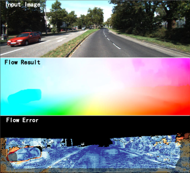
Figure 1: FastFlowNet can estimate accurate optical flow in real-time on embedded devices, which consumes only $\nicefrac{{1}}{{10}}$ computation of comparable networks to achieve on par performance.

Representative works of the first category include FlowNet [10] and FlowNet2 [11]. The pioneering FlowNet [10] designs two versions of models, named FlowNetS and FlowNetC. They both adopt the U-shape network. Specifically, FlowNetS only concatenates two input images while FlowNetC also contains a correlation layer. The successor FlowNet2 [11] further cascades multiple FlowNet models and employs carefully designed learning schedules on multiple datasets. FlowNet2 shows that CNNs can learn to estimate accurate optical flow with orders of magnitude faster than traditional competitors. However, these networks typically use a large number of channels in low resolutions for feature encoding, resulting in large model sizes, e.g., FlowNet2 containing more than 160M parameters. Moreover, the correlation layer in FlowNetC locates at a relative high resolution with large search radius, which leads to heavy computation burden. Both shortcomings have hindered them for lightweight mobile applications.

On the other hand, some approaches attempt to estimate residual flow among decomposed spatial levels where SPyNet [12] may be the first one in this category. SPyNet first constructs image pyramids, then concatenates the upsampled prior flow, first image and warped second image to estimate residual flow fields in a coarse-to-fine manner. Since each sub-module is only responsible for the small magnitude residual flow, SPyNet [12] can achieve the accuracy of FlowNet [10] with only 1.2M parameters. Almost at the same time, PWC-Net [13] and LiteFlowNet [14] replace image pyramids with better feature pyramids and introduce the correlation layer into each spatial level for better correspondence representation. Highly ranked results confirm the effectiveness of coarse-to-fine based approaches. As a result, following works appeared along this line of research [15, 16, 17, 18, 19].

Most recent works on optical flow [17, 19, 20] have focused almost exclusively on pursuing accuracy, the resulting methods with intensive computation are hardly deployed to energy-constrained embedded devices, such as unmanned aerial vehicles (UAV) and mobile phones. For example, as we show later, the efficient LiteFlowNet [14] barely breaks the 1 FPS barrier when inferring Sintel resolution images ($1024\times 436$) on Jetson TX2, which is still far from practical deployment.

To speed up accurate optical flow estimation and facilitate practical applications, we propose a lightweight and fast network, termed FastFlowNet in this paper. Our model is based on the widely used coarse-to-fine residual structure and we improve it on three aspects: 1) pyramid feature extraction, 2) cost volume construction and 3) optical flow decoding, covering all components of flow estimation pipeline.

First, we present a head enhanced pooling pyramid (HEPP) feature extractor, which uses convolution layers at higher levels while adopting parameter-free pooling at other lower levels. This efficient module can be viewed as a combination of feature pyramid in PWC-Net [13] and pooling pyramid of SPyNet [12], which aims to extract good matching features with considerably reduced parameters and computation. Second, recent studies [13, 19] have shown that increasing the search radius of the correlation layer can improve flow accuracy. However, feature channels of the cost volume are squared in terms of the search radius and computation complexity of following decoder network is 4th power of the search radius. In FastFlowNet, we keep the search radius to be 4 as in PWC-Net [13] for perceiving large movement. Differently, to reduce computation burden, we down sample feature channels in large residual regions and propose a new center dense dilated correlation (CDDC) layer for constructing compact cost volume. Our motivation is that residual flow distributions are more focused on small motions, and experiments show that CDDC behaves better than other compression methods. Third, we observe that flow decoders at each pyramid level occupy a relatively large proportion of parameters and computation as for the whole network. To further reduce computation and meanwhile retain superior performance, we build a new shuffle block decoder (SBD) module referring to the lightweight ShuffleNet [21], for its low computation budget and high classification precision. Different from ShuffleNet [21] as a backbone network, our SBD module is employed for regressing optical flow, which is only located in the middle part of decoder network. The overall architecture of FastFlowNet is illustrated in Fig. 2.

Based on the above improvements, our proposed network can achieve impressive performance on the Sintel [22] and KITTI [23] benchmarks with significantly reduced computation cost. In particular, FastFlowNet runs $3\times$ faster than PWC-Net [13] with $\nicefrac{{1}}{{7}}$ computation; and $5\times$ faster than LiteFlowNet [14] with $\nicefrac{{1}}{{13}}$ computation when predicting quarter resolution flow fields. Moreover, it only contains 1.37M parameters which is as light as SPyNet [12], but behaves much better with $5\times$ speed up, confirming state-of-the-art size-accuracy trade-off. Thanks to the coarse-to-fine structure, FastFlowNet can naturally trade accuracy for speed according to specific robotic applications. For example, our model can process $1024\times 436$ resolution images within a range of $5.7$-$26$ FPS on a single Jetson TX2 GPU. To our knowledge, FastFlowNet represents the first real-time solution for accurate optical flow on embedded devices.

II Related work

FlowNet [10] is the first work to use CNNs for optical flow estimation. It propose two variants of FlowNetS and FlowNetC together with the synthetic FlyingChairs dataset for end-to-end training. The improved version FlowNet2 [11] fuses cascaded FlowNets with a small displacement module, and uses FlyingThings3D [24] dataset for a further fine-tuning schedule. These encoder-decoder based networks have exceeded variational solutions with orders of magnitude faster speed. However, these models are not sufficiently compact and fast for mobile applications.

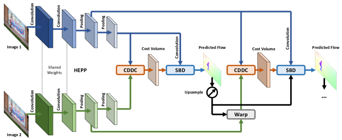
Figure 2: Architecture overview of the proposed FastFlowNet. HEPP, CDDC and SBD are efficient modules for extracting pyramid feature, constructing cost volume and regressing optical flow respectively. Only two levels are shown here for clarity.

Inspired by the traditional image pyramid, SPyNet [12] estimates residual flow in decomposed spatial levels with only 1.2M parameters, by sacrificing some performance accuracy. Following the coarse-to-fine residual structures, i.e., PWC-Net [13] and LiteFlowNet [14] employ feature pyramid, warping and correlation in each level to achieve good accuracy with a reduced number of parameters, representing the most efficient optical flow architecture.

Most recent works on optical flow focus on improving accuracy. IRR-PWC [15] shares the flow decoder and context network among all spatial scales for joint optical flow and occlusion estimation. HD3-Flow [16] decomposes contiguous flow fields into discrete grids and adopts a better backbone. FDFlowNet [18] employs better U-shape network and partial fully connected flow estimators for efficient inference. MaskFlowNet [17] adds additional occlusion mask module into PWC-Net [13] and uses cascaded refinement. Recently, RAFT [20] outperforms other approaches by first calculating all-pairs similarity and then performing iterations at a high resolution. The price is that it incurs significantly larger computation burden. We instead pay more attention to designing a compact model while retaining good optical flow accuracy here.

III Our method

III-A Overview of the Approach

Given two time-adjacent input images $I_{1},I_{2}\in\mathbb{R}^{H\times W\times 3}$, our proposed FastFlowNet exploits the coarse-to-fine residual structure to estimate gradually refined optical flow $F^{l}\in\mathbb{R}^{H^{l}\times W^{l}\times 2},l=6,5,\ldots,2$. But it is extensively reformed to accelerate inference by properly reducing parameters and computation cost. To this end, we first replace the dual convolution feature pyramid in PWC-Net [13] with the head enhanced pooling pyramid for enhancing high resolution pyramid feature and reducing model size. Then we propose a novel center dense dilated correlation layer for constructing compact cost volume while keeping the large search radius. Finally, new shuffle block decoders are employed at each pyramid level to regress optical flow with significantly cheaper computation. The structure details of the model are listed in Table I.

III-B Head Enhanced Pooling Pyramid

Traditional methods [25, 7] apply image pyramid to optical flow estimation for speeding up optimization or dealing with large displacement. SPyNet [12] transfers this classical paradigm and first introduces the pooling based image pyramid to deep models. Since raw images are variant to illumination changes and the fixed pooling pyramid is vulnerable to noise [26], such as shadows and reflection, PWC-Net [13] and LiteFlowNet [14] replace it by learnable feature pyramids with significant improvement. Concretely, they gradually expands feature channels while shrinking spatial size by half to extract robust matching features.

However, large channel numbers in low resolutions result in a large number of parameters. Moreover, it can be redundant for the coarse-to-fine structure, since low level pyramid features are only responsible to estimate coarse flow fields. Thus, we combine the feature pyramid at high levels with a pooling pyramid at other lower levels to obtain both strengths as shown in Fig. 2. On the other hand, high resolution pyramid features are relatively shallow in the PWC-Net, as each pyramid level only contains two convolutions with 3$\times$3 kernel that has small receptive field. Therefore, we add one more convolution at high levels to intensify pyramid features with a small extra cost. By balancing computation among different scales, we have presented a head enhanced pooling pyramid feature extractor as listed in the top of Table I. Like FlowNetC, PWC-Net and LiteFlowNet, HEPP generates six pyramid levels from $\nicefrac{{1}}{{2}}$ resolution (level 1) to $\nicefrac{{1}}{{64}}$ resolution (level 6) by a scale factor of 2.

III-C Center Dense Dilated Correlation

One crucial step in modern optical flow architectures is to calculate feature correspondence by the inner product based correlation layer [10]. Given two pyramid features of ${\rm f}_{1}^{l},{\rm f}_{2}^{l}$ in level $l$, like many coarse-to-fine residual approaches, we first adopt the bilinear interpolation based warping operation [12, 11] to warp the second feature ${\rm f}_{2}^{l}$ according to $2\times$ upsampled previous flow field ${\rm up_{2}}(F^{l+1})$. The warped target feature ${\rm f}_{\rm warp}^{l}$ can significantly reduce displacement caused by large motions, which helps to narrow the search region and simplify the task to estimate relatively small residual flow. Recent models [13][14] construct cost volume by correlating source features with corresponding warped target features within a local square area that can be formulated as

$$c^{l}({\bf x},{\bf d})={\rm f}_{1}^{l}({\bf x})\cdot{\rm f}_{\rm warp}^{l}({\bf x}+{\bf d})/N,\,{\bf d}\in[-r,r]\times[-r,r]$$ (1)

where $\bf x$ and $\bf d$ represent spatial and offset coordinates. $N$ is the length of input features. $r$ means search radius; and $\cdot$ stands for inner product.

Existing works [13, 19] have shown that increasing the search radius when building the cost volume can lead to lower end-point error during both training and testing, especially for large displacement cases. However, feature channels of the cost volume are squared in terms of the search radius and computation complexity of following decoder network becomes fourth power. As shown in Fig. 3a, many flow networks [13, 18, 15, 16] set $r=4$, and the resulting large computation burden has impeded low-power applications. A simple way to reduce computation cost is to decrease $r$, such as setting $r=3$ in Fig .3b. It can reduce cost volume features from 81 to 49, however this method is at the expense of sacrificing perception range and accuracy.

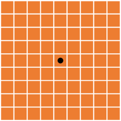
(a) $r=4$

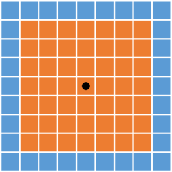
(b) $r=3$

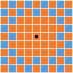
(c) CDDC

Figure 3: Different approaches for constructing the cost volume. Orange squares represent considered search grids. (a) and (b) are traditional square matching costs while (c) is the new proposed center dense dilated cost volume.

Inspired by the atrous spatial pyramid pooling (ASPP) module in DeepLabv3 [27], we propose a novel center dense dilated correlation (CDDC) layer that samples search grids densely around the center while down sampling grid points in large motion areas as shown in Fig. 3c.

Different from ASPP which uses parallel atrous convolutions to capture multi-scale context information, our proposed CDDC is designed to reduce computation when constructing large radius cost volume. In FastFlowNet, it outputs 53 feature channels which has similar computation budget with traditional $r=3$ setting. Our motivation is that the residual flow distribution is more focused on small motions. Our experiments show that CDDC behaves better than the naive compression method.

TABLE I: Architecture of FastFlowNet. HEPP, MFC, SBD represents head enhanced pooling pyramid, multiple feature construction and shuffle block decoder. MFC and SBD share the same structure across all pyramid levels, thus only level 5 are listed for brevity. ‘Pool’ stands for average pooling. Fconv5_2, fconv5_3 and fconv5_4 are convolutions with group $=$3. ‘Shuffle’ means the channel shuffle operation [21]. Convolution layers except upconv6 (deconvolution) and fconv5_7 are followed by a LeakyReLU activation.

	Layer Name	Kernel	Stride	Input	Ch I/O
HEPP	pconv1_1	3$\times$3	2	img1 or img2	3/16
	pconv1_2	3$\times$3	1	pconv1_1	16/16
	pconv2_1	3$\times$3	2	pconv1_2	16/32
	pconv2_2	3$\times$3	1	pconv2_1	32/32
	pconv2_3	3$\times$3	1	pconv2_2	32/32
	pconv3_1	3$\times$3	2	pconv2_3	32/64
	pconv3_2	3$\times$3	1	pconv3_1	64/64
	pconv3_3	3$\times$3	1	pconv3_2	64/64
	pool4	2$\times$2	2	pconv3_3	64/64
	pool5	2$\times$2	2	pool4	64/64
	pool6	2$\times$2	2	pool5	64/64
MFC	upconv6	4$\times$4	1/2	flow6	2/2
	warp5	-	-	pool5b,upconv6	64,2/64
	cddc5	1$\times$1	1	pool5a,warp5	64,64/53
	rconv5	3$\times$3	1	pool5a	64/32
	concat5	rconv5 + cddc5 + upconv6			32,53,2/87
SBD	fconv5_1	3$\times$3	1	concat5	87/96
	fconv5_2	3$\times$3	1	fconv5_1	3$\times$32/3$\times$32
	shuffle5_2	-	-	fconv5_2	3$\times$32/32$\times$3
	fconv5_3	3$\times$3	1	shuffle5_2	3$\times$32/3$\times$32
	shuffle5_3	-	-	fconv5_3	3$\times$32/32$\times$3
	fconv5_4	3$\times$3	1	shuffle5_3	3$\times$32/3$\times$32
	shuffle5_4	-	-	fconv5_4	3$\times$32/32$\times$3
	fconv5_5	3$\times$3	1	shuffle5_4	96/64
	fconv5_6	3$\times$3	1	fconv5_5	64/32
	fconv5_7	3$\times$3	1	fconv5_6	32/2

III-D Shuffle Block Decoder

After building the cost volume, coarse-to-fine models usually concatenate context features, cost volume and upsampled previous flow as inputs for the following decoder networks. Due to each pyramid level, the decoder part takes up most parameters and computation of the whole network. Thus, better speed-accuracy trade-off is critically important.

PWC-Net [13] shows that the dense connected flow decoder can improve accuracy after fine-tuning on the FlyingThings3D [24] dataset at the price of increasing the model size and computation. LiteFlowNet [14] uses sequential connected flow estimator and also shows improved performance. To achieve better trade-off between these two schemes, FDFlowNet [18] employs the partial fully connected structure. However, all these methods can not well support real-time inference on embedded systems.

Thanks to the compact cost volume built by CDDC, we can directly decrease maximal feature channels in decoder network from 128 to current 96 without issues. To further reduce computation and model size, we reform the middle three 96-channel convolutions into group convolutions followed by channel shuffle operations, which we term ‘shuffle block’. Different from ShuffleNet [21] as a backbone network, our shuffle block decoder is employed for regressing optical flow. As listed in the bottom of Table I, each decoder network contains three shuffle blocks with group $=3$, which can efficiently reduce computation with marginal drops in accuracy.

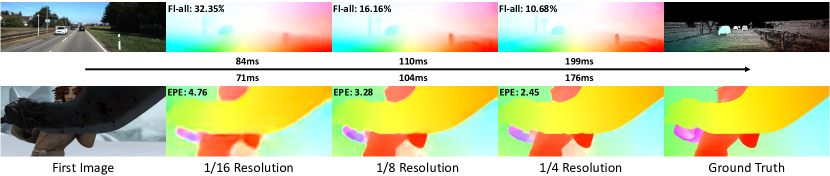
Figure 4: Visual examples of anytime inference. FastFlowNet can naturally trade speed for accuracy according to specific robotic applications. Black arrow means inference timeline which is measured on an embedded Jetson TX2 GPU.

TABLE II: Ablation study on structure variants with different pyramid feature extractor, cost volume constructor and optical flow decoder. Flow accuracy is measured by end point error. FLOPs are calculated on Sintel resolution images.

Pyramid	Cost	Decoder	Sintel	KITTI	Params.	FLOPs
conv	$r=4$	$g=1$	3.12	2.37	4.23M	28.2G
conv+pool	$r=4$	$g=1$	3.00	2.25	3.22M	27.7G
HEPP	$r=4$	$g=1$	2.92	2.13	3.27M	28.3G
HEPP	$r=3$	$g=1$	2.93	2.33	2.18M	19.1G
HEPP	CDDC	$g=1$	2.95	2.18	2.20M	19.2G
HEPP	CDDC	$g=2$	3.04	2.22	1.57M	14.0G
HEPP	CDDC	$g=3$	3.11	2.29	1.37M	12.2G
HEPP	CDDC	$g=4$	3.22	2.47	1.26M	11.3G
HEPP	CDDC	$g=6$	3.35	2.59	1.16M	10.4G

III-E Loss Function

Since FastFlowNet has the same pyramid scales as FlowNet [10] and PWC-Net [13], we adopt the same multi-scale L2 loss for training

$$L_{epe}=\sum_{l=2}^{6}\alpha_{l}\sum_{\bf x}|F^{l}({\bf x})-F_{gt}^{l}({\bf x})|_{2}$$ (2)

where $|\cdot|_{2}$ computes L2 norm between predicted and ground-truth flow fields. When fine-tuning on datasets with real scene structure, such as KITTI, we use following robust loss

$$L_{robust}=\sum_{l=2}^{6}\alpha_{l}\sum_{\bf x}(|F^{l}({\bf x})-F_{gt}^{l}({\bf x})|+\epsilon)^{q}$$ (3)

where $|\cdot|$ denotes L1 norm, $\epsilon=0.01$ is a small constant and $q<1$ makes loss more robust for large magnitude outliers. For fair comparison with previous methods [10, 11, 13, 14], weights in Eq. (2) and Eq. (3) are set to $\alpha_{6}=0.32,\alpha_{5}=0.08,\alpha_{4}=0.02,\alpha_{3}=0.01$ and $\alpha_{2}=0.005$.

TABLE III: Performance comparison on benchmark datasets. Speed and computation are measured on Sintel resolution images. Results in parentheses are that of networks being trained on the same dataset. Default accuracy metric is the end-point error.

Method	Sintel Clean		Sintel Final		KITTI 2012		KITTI 2015			Params	FLOPs	Time (s)
	train	test	train	test	train	test	train	train (Fl-all)	test (Fl-all)	(M)	(G)	1080Ti	TX2
FlowNetC [10]	4.31	7.28	5.87	8.81	9.35	-	-	-	-	39.18	6055.3	0.029	0.427
FlowNetC-ft	(3.78)	6.85	(5.28)	8.51	8.79	-	-	-	-	39.18	6055.3	0.029	0.427
FlowNet2 [11]	2.02	3.96	3.14	6.02	4.09	-	10.06	30.37%	-	162.52	24836.4	0.116	1.547
FlowNet2-ft	(1.45)	4.16	(2.01)	5.74	(1.28)	1.8	(2.30)	(8.61%)	11.48%	162.52	24836.4	0.116	1.547
SPyNet [12]	4.12	6.69	5.57	8.43	9.12	-	-	-	-	1.20	149.8	0.050	0.918
SPyNet-ft	(3.17)	6.64	(4.32)	8.36	(4.13)	4.7	-	-	35.07%	1.20	149.8	0.050	0.918
PWC-Net [13]	2.55	-	3.93	-	4.14	-	10.35	33.67%	-	8.75	90.8	0.034	0.485
PWC-Net-ft	(2.02)	4.39	(2.08)	5.04	(1.45)	1.7	(2.16)	(9.80%)	9.60%	8.75	90.8	0.034	0.485
LiteFlowNet[14]	2.48	-	4.04	-	4.00	-	10.39	28.50%	-	5.37	163.5	0.055	0.907
LiteFlowNet-ft	(1.35)	4.54	(1.78)	5.38	(1.05)	1.6	(1.62)	(5.58%)	9.38%	5.37	163.5	0.055	0.907
PWC-Net-small	2.83	-	4.08	-	-	-	-	-	-	4.08	-	0.024	-
LiteFlowNetX	3.58	-	4.79	-	6.38	-	15.81	34.90%	-	0.90	-	0.035	-
FastFlowNet	2.89	-	4.14	-	4.84	-	12.24	33.10%	-	1.37	12.2	0.011	0.176
FastFlowNet-ft	(2.08)	4.89	(2.71)	6.08	(1.31)	1.8	(2.13)	(8.21%)	11.22%	1.37	12.2	0.011	0.176

IV Experiments

IV-A Implementation Details

To compare FastFlowNet with other networks, we follow the two-stage training strategy proposed in FlowNet2 [11]. Ground truth optical flow is divided by 20 and down sampled as supervision at different levels. Since final flow prediction is in a quarter resolution, we use bilinear interpolation to obtain the full resolution optical flow. During both training and fune-tuning, we use the same data augmentation methods as in [11], including mirror, translate, rotate, zoom, squeeze and color jitter. All our experiments are implemented in PyTorch and conducted on a machine equipped with 4 NVIDIA GTX 1080 Ti GPU cards. To compare performance of different optical flow models on mobile devices, we further evaluate inference time on the embedded Jetson TX2 GPU.

We first train FastFlowNet on FlyingChairs [10] using $S_{short}$ learning schedule [11], i.e., the learning rate is initially set to $1e-4$ and decays half at 300k, 400k and 500k iterations. We crop $320\times 448$ patches during data augmentation and adopt a batch size of 8. Then the model is fine-tuned on FlyingThings3D [24] using the $S_{fine}$ schedule [11], i.e., the learning rate is initially set to $1e-5$ and decays by half at 200k, 300k and 400k iterations. Random crop size is $384\times 768$ and the batch size is set to 4. The Adam [28] optimizer and multi-scale L2 loss in Eq. 2 are always used. We call the model FastFlowNet after above two-stage learning schedules whose results on Sintel and KITTI training sets are listed in Table III.

IV-B Ablation Study

To explore the efficient optical flow structure with low computation cost, we perform ablations on the pyramid feature extractor, cost volume constructor and optical flow decoder. Results of the gradually lightened models are listed in Table II. All variants are first trained on FlyingChairs and evaluated on Sintel Clean training sets. To test in large displacement cases, which are common when robots move forward or backward, they are fine-tuned on KITTI 2015 training subset for 5-fold cross-validation. Since change of inference time is not distinct based on our PyTorch implementation, we use FLOPs [29, 21] which means number of floating point multiply-add operations to measure real computation complexity. In Table II, ‘conv’ represents dual convolution feature pyramid used in PWC-Net, ‘conv+pool’ stands for combining dual convolution feature pyramid in top 3 levels with pooling pyramid in bottom 3 levels. Note that traditional $r=4$ cost volume has sequential connected flow decoders, whose maximal feature channel is 128 rather than 96, in order to make it fully convergent. $g=1$ means no grouping convolution without shuffle block in flow decoder.

Surprisingly, the lighter ‘conv+pool’ pyramid feature extractor behaves better than the traditional ‘conv’ method. Our analysis is that parameter-free average pooling may share gradients among different levels during back-propagation, which may have made pyramid features more robust to scale changes.

By replacing ‘conv+pool’ with HEPP, we can achieve better results with small additional overhead. Then, we decrease the search radius for constructing lightened $r=3$ cost volume to reduce computation. Flow accuracy on Sintel shows almost no change, while results on large displacement KITTI decline clearly. To mitigate performance degradation, we adopt CDDC to build a compact cost volume with larger receptive field at each pyramid level. Although it does not improve on Sintel training which contains many small movements, it works better on the more challenging KITTI 2015 validation set.

Finally, we employ SBD for further compression on parameters and computation. In Table III, we gradually lighten the network by setting incremental group numbers in SBD. It can be seen that computation reduction becomes relatively small when $g>3$, whereas clear performance degradation appears. Thus, we adopt $g=3$ in FastFlowNet which shows a better computation-accuracy trade-off.

IV-C MPI Sintel

When fine-tuning on the Sintel [22] training sets, we crop $320\times 768$ patches and set the batch size to 4. Robust loss in Eq. 3 is adopted with $q=0.4$. Like PWC-Net, we set the initial learning rate to $5e-5$ and change it to $3e-5$, $2e-5$ and $1e-5$ every 150k iterations in total 600k iterations, where the learning rate decays to zero in each period. We report results on the Sintel test sets by submitting predictions to the MPI Sintel online benchmark, which are listed in Table III. For mobile applications, we also measure computation burden of different networks in FLOPs and real inference time on both desktop GTX 1080Ti GPU and embedded Jetson TX2. All experiments are conducted in PyTorch for fair comparison.

In Table III, FastFlowNet outperforms FlowNetC [10] in all items due to the advanced coarse-to-fine residual structure. It runs $2.5\times$ faster than FlowNetC on both GTX 1080Ti and Jetson TX2 with $500\times$ less computation. The reason why competition complexity is not proportional to inference time is that correlation and warping layers have large memory access cost (MAC) while they are low FLOPs operations.

FastFlowNet outperforms SPyNet [12] by $26.4\%$ and $27.3\%$ on Sintel Clean and Final test sets respectively. Although containing slightly more parameters, our network runs $5\times$ faster with $12\times$ less computation. Compared with the state-of-the-art LiteFlowNet [14], we can approach $90\%$ of its performance with $13.4\times$ less (only 12.2 GFLOPs) computation cost.

To further verify the effectiveness of the proposed flow architecture, we compare FastFlowNet with compact versions of PWC-Net [13] and LiteFlowNet [14] provided in their papers. PWC-Net-small is the small version of PWC-Net by dropping dense connections in flow decoders; and LiteFlowNetX is the small variant by shrinking convolution channels in feature pyramid and flow estimators. We can see that FastFlowNet achieves almost the same good results with PWC-Net-small on Sintel training datasets after two-stage pretraining, while being additional $3\times$ samller and $2\times$ faster.

IV-D KITTI

To test the proposed architecture on more challenging large displacement real world data, we fine-tune FastFlowNet on mixed KITTI 2012 [30] and KITTI 2015 [23] training sets. Like [11, 13, 14], we crop $320\times 896$ patches and adopt a batch size of 4. The same fine-tuning schedule on Sintel is employed and $q$ in robust loss is set to $0.2$ for outlier suppression. To adapt to driving scenes, spatial augmentation methods of rotate, zoom and squeeze are skipped with a probability of $0.5$ as [13, 14]. Then we evaluate the fine-tuned FastFlowNet on the online KITTI benchmarks which are listed in Table III.

Compared with the encoder-decoder based FlowNet2 [11], our model can achieve on par or better results on KITTI test datasets while being $120\times$ smaller and $10\times$ faster.

We can achieve similar accuracy compared to PWC-Net [13] with $7.5\times$ less multiply-add computation cost. For LiteFlowNetX which simply reduces feature channels, our proposed HEPP, CDDC and SBD modules work better on all metrics confirming effectiveness of our contribution. Some visual results in anytime setting [31, 32] are shown in Fig. 4.

V Conclusion

In this paper, we have proposed a fast and lightweight network for accurate optical flow estimation for mobile applications. Our method is based on the well-known coarse-to-fine structure and is extensively reformed to accelerate inference by properly reducing parameters and computation. The proposed head enhanced pooling pyramid, center dense dilated correlation and shuffle block decoder are efficient modules for pyramid feature extraction, cost volume construction and optical flow decoding, which covers all components of flow estimation pipeline. We have evaluated each component on both synthetic Sintel and real-world KITTI datasets to verify their effectiveness. The proposed FastFlowNet can be directly plugged into any optical flow based robotic vision systems with much less resource consumption, achieving good accuracy.

References

- [1] K. Shuang, Y. Huang, Y. Sun, Z. Cai, and H. Guo, “Fine-grained motion representation for template-free visual tracking,” in Proc. Winter Conf. Applications Comp. Vis., pp. 660–669, 2020.
- [2] C. Wang, T. Ji, T. Nguyen, and L. Xie, “Correlation flow: Robust optical flow using kernel cross-correlators,” in Proc. Int. Conf. Robotics Automation, pp. 836–841, 2018.
- [3] K. Souhila and A. Karim, “Optical flow based robot obstacle avoidance,” Int. J. Advanced Robotic Systems, vol. 4, no. 1, p. 2, 2007.
- [4] J. Chang, A. Tejero-de-Pablos, and T. Harada, “Improved optical flow for gesture-based human-robot interaction,” in Proc. Int. Conf. Robotics Automation, pp. 7983–7989, 2019.
- [5] X. Yang, L. Kong, and J. Yang, “Unsupervised motion representation enhanced network for action recognition,” in Proc. IEEE Int. Conf. Acoustics, Speech and Signal Process., 2021.
- [6] B. K. P. Horn and B. G. Schunck, “Determining optical flow,” in Artif. Intell., 1981.
- [7] T. Brox and J. Malik, “Large displacement optical flow: Descriptor matching in variational motion estimation,” in IEEE Trans. Pattern Anal. Mach. Intell., 2011.
- [8] C. Zach, T. Pock, and H. Bischof, “A duality based approach for realtime tv-l1 optical flow,” in Pattern Recognition (F. A. Hamprecht, C. Schnörr, and B. Jähne, eds.), 2007.
- [9] T. Kroeger, R. Timofte, D. Dai, and L. Van Gool, “Fast optical flow using dense inverse search,” in Proc. Eur. Conf. Comp. Vis. (B. Leibe, J. Matas, N. Sebe, and M. Welling, eds.), 2016.
- [10] P. Fischer, A. Dosovitskiy, E. Ilg, P. Häusser, C. Hazirbas, V. Golkov, P. van der Smagt, D. Cremers, and T. Brox, “Flownet: Learning optical flow with convolutional networks,” in Proc. IEEE Int. Conf. Comp. Vis., 2015.
- [11] E. Ilg, N. Mayer, T. Saikia, M. Keuper, A. Dosovitskiy, and T. Brox, “Flownet 2.0: Evolution of optical flow estimation with deep networks,” in Proc. IEEE Conf. Comp. Vis. Patt. Recogn., 2017.
- [12] A. Ranjan and M. J. Black, “Optical flow estimation using a spatial pyramid network,” in Proc. IEEE Conf. Comp. Vis. Patt. Recogn., 2017.
- [13] D. Sun, X. Yang, M.-Y. Liu, and J. Kautz, “PWC-Net: CNNs for optical flow using pyramid, warping, and cost volume,” in Proc. IEEE Conf. Comp. Vis. Patt. Recogn., 2018.
- [14] T.-W. Hui, X. Tang, and C. Change Loy, “Liteflownet: A lightweight convolutional neural network for optical flow estimation,” in Proc. IEEE Conf. Comp. Vis. Patt. Recogn., 2018.
- [15] J. Hur and S. Roth, “Iterative residual refinement for joint optical flow and occlusion estimation,” in Proc. IEEE Conf. Comp. Vis. Patt. Recogn., 2019.
- [16] Z. Yin, T. Darrell, and F. Yu, “Hierarchical discrete distribution decomposition for match density estimation,” in Proc. IEEE Conf. Comp. Vis. Patt. Recogn., June 2019.
- [17] S. Zhao, Y. Sheng, Y. Dong, E. I.-C. Chang, and Y. Xu, “Maskflownet: Asymmetric feature matching with learnable occlusion mask,” in Proc. IEEE Conf. Comp. Vis. Patt. Recogn., 2020.
- [18] L. Kong and J. Yang, “Fdflownet: Fast optical flow estimation using a deep lightweight network,” in Proc. IEEE Int. Conf. Image Process., 2020.
- [19] M. Hofinger, S. R. Bulò, L. Porzi, A. Knapitsch, T. Pock, and P. Kontschieder, “Improving optical flow on a pyramid level,” in Proc. Eur. Conf. Comp. Vis., 2020.
- [20] Z. Teed and J. Deng, “Raft: Recurrent all-pairs field transforms for optical flow,” in Proc. Eur. Conf. Comp. Vis., 2020.
- [21] X. Zhang, X. Zhou, M. Lin, and J. Sun, “Shufflenet: An extremely efficient convolutional neural network for mobile devices,” in Proc. IEEE Conf. Comp. Vis. Patt. Recogn., 2018.
- [22] D. J. Butler, J. Wulff, G. B. Stanley, and M. J. Black, “A naturalistic open source movie for optical flow evaluation,” in Proc. Eur. Conf. Comp. Vis., 2012.
- [23] M. Menze and A. Geiger, “Object scene flow for autonomous vehicles,” in Proc. IEEE Conf. Comp. Vis. Patt. Recogn., pp. 3061–3070, 2015.
- [24] N. Mayer, E. Ilg, P. Häusser, P. Fischer, D. Cremers, A. Dosovitskiy, and T. Brox, “A large dataset to train convolutional networks for disparity, optical flow, and scene flow estimation,” in Proc. IEEE Conf. Comp. Vis. Patt. Recogn., 2016.
- [25] J. yves Bouguet, “Pyramidal implementation of the lucas kanade feature tracker,” Intel Corporation, Microprocessor Research Labs, 2000.
- [26] T. Brox, A. Bruhn, N. Papenberg, and J. Weickert, “High accuracy optical flow estimation based on a theory for warping,” in Proc. Eur. Conf. Comp. Vis., 2004.
- [27] L.-C. Chen, G. Papandreou, F. Schroff, and H. Adam, “Rethinking atrous convolution for semantic image segmentation,” arXiv: Comp. Res. Repository, vol. abs/1706.05587, 2017.
- [28] D. P. Kingma and J. Ba, “Adam: A method for stochastic optimization,” in Proc. Int. Conf. Learn. Representations, 2015.
- [29] A. G. Howard, M. Zhu, B. Chen, D. Kalenichenko, W. Wang, T. Weyand, M. Andreetto, and H. Adam, “Mobilenets: Efficient convolutional neural networks for mobile vision applications,” arXiv: Comp. Res. Repository, vol. abs/1704.04861, 2017.
- [30] A. Geiger, P. Lenz, and R. Urtasun, “Are we ready for autonomous driving? the kitti vision benchmark suite,” in Proc. IEEE Conf. Comp. Vis. Patt. Recogn., 2012.
- [31] Y. Wang, Z. Lai, G. Huang, B. H. Wang, L. Van Der Maaten, M. Campbell, and K. Q. Weinberger, “Anytime stereo image depth estimation on mobile devices,” in Proc. Int. Conf. Robotics Automation, 2019.
- [32] P. L. Dovesi, M. Poggi, L. Andraghetti, M. Martí, H. Kjellström, A. Pieropan, and S. Mattoccia, “Real-time semantic stereo matching,” in Proc. Int. Conf. Robotics Automation, 2020.