Predictive Visual Tracking: A New Benchmark and Baseline Approach

Abstract

As a crucial robotic perception capability, visual tracking has been intensively studied recently. In the real-world scenarios, the onboard processing time of the image streams inevitably leads to a discrepancy between the tracking results and the real-world states. However, existing visual tracking benchmarks commonly run the trackers offline and ignore such latency in the evaluation. In this work, we aim to deal with a more realistic problem of latency-aware tracking. The state-of-the-art trackers are evaluated in the aerial scenarios with new metrics jointly assessing the tracking accuracy and efficiency. Moreover, a new predictive visual tracking baseline is developed to compensate for the latency stemming from the onboard computation. Our latency-aware benchmark can provide a more realistic evaluation of the trackers for the robotic applications. Besides, exhaustive experiments have proven the effectiveness of the proposed predictive visual tracking baseline approach. Our code is on  https://github.com/vision4robotics/LAE-PVT-master.

I Introduction

Visual tracking, one of the fundamental perception tasks for mobile robots, has introduced various real-world applications [1, 2, 3]. In the past decade, visual tracking benchmarks [4, 5, 6, 7] have generally focused on the offline evaluation, i.e., they query the state of the object on each image frame with a ground-truth annotation. In the real world, however, when the algorithm finishes processing a captured frame, the surrounding environment has changed in varying degrees, i.e., the output of the tracker is always outdated.

Especially for Unmanned Aerial Vehicle (UAV) tracking applications, such latency can be more detrimental due to: 1) the scarce onboard computation resource ends up in longer processing time, i.e., more remarkable latency, 2) the fast motion scenarios on UAV cause drastic state changes of the target objects in a very short time. Consequently, the delayed tracking results can jeopardize the robot perception and planning modules. In visual tracking community, many attempts are made to improve the tracking accuracy and robustness on the existing offline benchmarks [8, 9, 10, 11]. Although the performance has been largely improved, a latency-aware benchmark/approach jointly considering the accuracy as well as latency is more desirable for the robotics community.

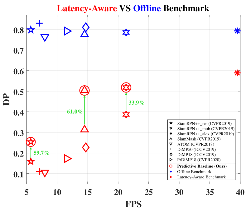
Figure 1: Performance of the state-of-the-art trackers with offline latency-free and online latency-aware benchmarks on DTB70 [12]. The distance precision (DP) is employed for evaluation. The same shape indicates the same tracker, e.g., star for SiamRPN++ [9] with ResNet50 as backbone. Blue denotes the results on the offline benchmark. Red means the results on the latency-aware benchmark. Our predictive tracking baseline is marked out by red circles, where the original performance is improved by a considerable margin, denoted by green arrows and percentages.

In this work, different from the offline evaluation querying the state of the object on each image, we propose a latency-aware evaluation (LAE) approach by querying the state of the target object at each timestamp. In our settings, the onboard computation would introduce extra time, therefore, the trackers have to output the future states of the object, to compensate for the latency. Essentially, visual tracking has become a joint perception and forecasting task, whereas the offline tracking is solely a perception mission. We name such a novel task as predictive visual tracking (PVT). Compared to the offline tracking, PVT is more realistic and can yield the states of the object in real time, yet suffers from increased uncertainties and is more challenging.

In the context of predictive visual tracking, we firstly benchmark several state-of-the-art trackers [13, 9, 10, 11, 14] against the latency-aware criteria on a high-end UAV processor. As illustrated in Fig. 1, compared to the offline latency-free benchmark (in blue color), the tracking performance is greatly lowered in the latency-aware settings (in red color), especially for the trackers with low speed. Moreover, we propose a novel and effective plug-in prediction module (in red circles). Our contributions are three-fold:

• A novel task of joint tracking and forecasting, i.e., predictive visual tracking (PVT), is proposed to bridge the gap between computer vision and real-world robotics.

• A new latency-aware evaluation (LAE) benchmark is developed to comprehensively evaluate the trackers in terms of both accuracy and efficiency.

• Exhaustive experiments have been extended on an onboard device to point out the urgent latency issue and validate the proposed PVT baseline.

To the best of our knowledge, we are the first to establish a realistic latency-aware benchmark in visual tracking. The results in Fig. 1 indicate the significance for the robotics and vision community to focus on PVT. We release our code and toolkit to facilitate further investigations for the community. Important notations used for deduction are shown in TABLE I for clear reference.

II Related Works

II-A Visual Tracking Approaches

Visual tracking aims to localize the object of interest in the image streams given solely the information of the target on the first frame. Current methods generally consider the tracking as a confidence regression problem: given the filter/template and the current frame, cross correlation is implemented and the location with the highest confidence score will be the output. Discriminative correlation filter (DCF)-based [15, 16, 17, 18, 19, 3] and Siamese network-based trackers [8, 9, 10, 11] are two main paradigms in visual tracking community. DCF-based trackers are highly efficient thanks to the fast Fourier transform (FFT) and are frequently used in robotics applications [20, 21, 22, 23, 24]. Yet there is still an obvious gap between their performance and that of deep learning methods. Siamese trackers have excellent performance but is much slower especially on the mobile robots with constrained calculation resources. In this work, we benchmark the advanced deep trackers in the latency-aware scenarios and try to improve the performance via a predictive baseline.

II-B Visual Tracking Benchmarks

Since OTB was proposed in 2013 [4], many visual object tracking datasets have been developed following the evaluation metrics in OTB, such as LaSOT [6], TrackingNet [25], GOT-10K [7], etc., in order to improve the diversity of the tracking scenarios. Moreover, multi-modality tracking [26, 27], first-person view tracking [28], day-and-night tracking [29], aerial tracking [5, 12] were also proposed to further boost the real-world applications of visual tracking. In addition to OTB protocol, VOT [30, 31, 32], an annual visual object tracking challenge, has employed a re-initialization scheme when encountering tracking failure. In a word, existing tracking benchmarks generally address the tracking accuracy and robustness in various tracking scenes, while neglecting the evaluation of the real-world latency introduced by the computation. In this work, we reformulate the evaluation protocol in visual tracking by jointly assessing the tracking accuracy and latency. We employ the aerial tracking benchmarks [5, 12, 33] captured by the real-world UAV for realistic evaluations.

II-C Latency in Perception

In the computer vision community, the problem of latency has been extensively studied. [34, 35, 36] proposed lightweight architectures to ease the computation. [3, 19] proposed efficient algorithms to decrease the running time. Researchers generally claim that the algorithm is real-time when the running speed is higher than the frame rates. However, even for the algorithms faster than the frame rates, the output is still not real-time since the state of the world has already changed when a specific frame is processed. [37] instantiated a benchmark of streaming object detection to highlight the importance of the latency in the real-time perception. Yet there is still no latency-aware benchmark and baseline approach in the area of visual object tracking, where latency issue is actually more critical.

TABLE I: List of the important notations in this work.

Symbol	Meaning	Dimension
$i$	World frame number	$\mathbb{R}$
$T$	Sequence length	$\mathbb{R}$
$k$	Serial number of the processed frame	$\mathbb{R}$
$j_{k}$	Input frame id for the tracker (World frame id of the processed frame)	$\mathbb{R}$
$K$	Total number of the processed frames	$\mathbb{R}$
$t_{\mathrm{g}}^{i}$	World timestamp	$\mathbb{R}$
$t_{\mathrm{r}}^{j_{k}}$	Tracker timestamp	$\mathbb{R}$
$\mathcal{T}^{j_{k}}$	Processing time of frame $j_{k}$	$\mathbb{R}$
$\psi(i)(=j_{h})$	Input frame id to be paired with frame $i$	$\mathbb{R}$
$\Delta t_{k}$	Time interval between two frames $j_{k+1}$ and $j_{k}$	$\mathbb{R}$
$\Delta t_{i}$	Time interval between two frames $i$ and $\psi{i}$	$\mathbb{R}$
$\Delta t_{h}$	Time interval between two frames $j_{h+1}$ and $j_{h}$	$\mathbb{R}$
$\mathbf{b}_{\mathrm{g}}^{i}$	Ground-truth bounding box in frame $i$	$\mathbb{R}^{1\times 4}$
$\mathbf{b}_{\mathrm{r}}^{j_{k}}$	Raw output bounding box in frame $j_{k}$	$\mathbb{R}^{1\times 4}$
$\hat{\mathbf{b}}_{\mathrm{r}}^{i}$	Final output bounding box to be evaluated	$\mathbb{R}^{1\times 4}$
$\mathbf{s}_{j_{k}}$	Updated object state in frame $j_{k}$	$\mathbb{R}^{8\times 1}$
$\hat{\mathbf{s}}_{j_{k}}$	Predicted object state in frame $j_{k}$	$\mathbb{R}^{8\times 1}$
$\mathbf{z}_{j_{k+1}}$	Measured (Tracked) object box in frame $j_{k+1}$	$\mathbb{R}^{4\times 1}$
$\mathbf{P}_{j_{k}}$	Updated covariance matrix in frame $j_{k}$	$\mathbb{R}^{8\times 8}$
$\hat{\mathbf{P}}_{j_{k}}$	Predicted covariance matrix in frame $j_{k}$	$\mathbb{R}^{8\times 8}$
$\mathbf{F}(\Delta t)$	Transition matrix for time interval $\Delta t$	$\mathbb{R}^{8\times 8}$
$\mathbf{Q}(\Delta t)$	Noise matrix for time interval $\Delta t$	$\mathbb{R}^{8\times 8}$
$\mathbf{K}_{j_{k}}$	Kalman gain for frame $j_{k}$	$\mathbb{R}^{4\times 4}$
$\mathbf{H}$	Slicing matrix	$\mathbb{R}^{4\times 8}$
$\mathbf{I}_{N}$	Identity matrix	$\mathbb{R}^{N\times N}$

III Latency-Aware Benchmark

III-A Ground-truth Reformulation

To query the object’s state at each timestamp, we firstly define a world frame rate $\kappa$ set as 30 frames/s (FPS). So the ground-truths $\mathbf{G}=[\mathbf{g}_{0},\mathbf{g}_{1},\dots,\mathbf{g}_{T-1}]\in\mathbb{R}^{6\times T}$ are:

$$\mathbf{g}_{i}=[i,\mathbf{b}_{\mathrm{g}}^{i},t_{\mathrm{g}}^{i}]^{\mathrm{T}}~{},$$ (1)

where $i$ and $T$ denote frame number and sequence length respectively, $\mathbf{b}_{\mathrm{g}}^{i}=[x_{i},y_{i},w_{i},h_{i}]$ indicates the ground-truth bounding box in the $i$-th frame, and $t_{\mathrm{g}}^{i}=\frac{i}{\kappa}$ is the world timestamp.

III-B Tracking Schedule

In the real-world tracking scenarios, a tracker faster than the world frame rate is able to process every captured frame. However, slow trackers with large latency can simply process the latest frame, discarding the frames captured during the calculation. The output results $\mathbf{R}=[\mathbf{r}_{0},\mathbf{r}_{1},\dots,\mathbf{r}_{K-1}]\in\mathbb{R}^{6\times K}$ of the tracker can be formulated as:

$$\mathbf{r}_{k}=[j_{k},\mathbf{b}_{\mathrm{r}}^{j_{k}},t_{\mathrm{r}}^{j_{k}}]^{\mathrm{T}}~{},$$ (2)

where $k$ denotes the $k$-th processed frames with a length of $K$ and $j_{k}$ denotes the world frame number. $\mathbf{b}_{\mathrm{r}}^{j_{k}}$ represents the output bounding box on frame ${j_{k}}$. $t_{\mathrm{r}}^{j_{k}}$ means the tracker timestamp, i.e., the time after the tracker finishes processing frame ${j_{k}}$. Specifically, define $\mathcal{T}^{j_{k}}$ as the time consumed by the tracker to process frame ${j_{k}}$, $t_{\mathrm{r}}^{j_{k}}$ can be calculated as:

$$t_{\mathrm{r}}^{j_{k}}=\sum_{x=0}^{k}\mathcal{T}^{j_{x}}~{}.$$ (3)

In this case, the latency-aware output $\mathbf{R}$ depends on ${j_{k}}$, i.e., which frame to be processed. This work considers ${j_{k}}$ as the latest available frame number as:

$$\mathcal{I}_{f},\mathcal{I}_{0},,\mathcal{I}_{1},,\mathcal{I}_{2},,\mathcal{I}_{3},\mathcal{I}_{4}$$ (4)

Remark 1: Due to the latency, the processed frame id $j_{k}$ could be nonconsecutive, i.e., $\mathbf{j}=[j_{0},j_{1},\dots,j_{K-1}]\subseteq[0,1,\dots,T-1]$. Consequently, the motion between frame $j_{k}$ and $j_{k+1}$ is much stronger, making latency-aware tracking more challenging $\mathcal{H}_{\phi(11)}$.

III-C Evaluation Process

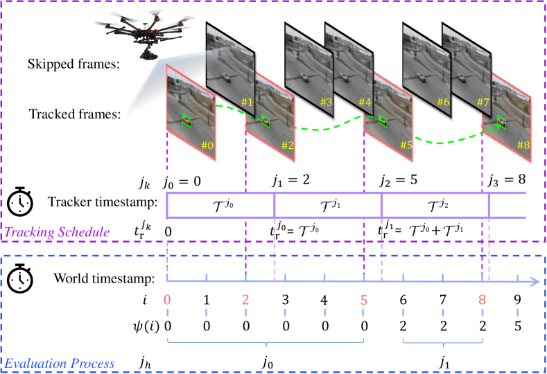
Figure 2: Example of the proposed latency-aware benchmark. If the tracker is slower than the world frame rate, some frames would be skipped. Also, there is a mismatch between the evaluated frame $i$ and the latest tracked frame $\psi(i)$. The tracking schedule and evaluation metric are exhibited in purple and blue dotted lines, respectively.

Different from offline benchmark pairing the ground-truth in the $i$-th frame with the output in the $i$-th frame, the proposed LAE benchmark pairs ground-truth $\mathbf{b}^{i}_{\mathrm{g}}$ at time $t_{\mathrm{g}}^{i}$ with the latest output result $\mathbf{b}_{\mathrm{r}}^{\psi(i)}$ where $\psi(i)$ is:

$$\psi(i)=\left\{\begin{array}[]{crl}0&,&{t_{\mathrm{g}}^{i}<t_{\mathrm{r}}^{j_{0}}}\\ \mathop{\arg\max}_{j_{k}}\ t_{\mathrm{r}}^{j_{k}}\leq t_{\mathrm{g}}^{i}&,&{\mathrm{others}}\end{array}\right.~{}.$$ (5)

Remark 2: In practice, there is no “in time” tracking results. Since $\mathcal{T}^{j_{k}}>0$, the output time for frame $i$ will definitely satisfy $t_{\mathrm{r}}^{i}>t_{\mathrm{g}}^{i}$. This makes the latest input frame id $\psi(i)<i\ (i>0)$. Hence, the output will be at least one frame behind the ground-truth. Figure 2 illustrated the overall picture of the processing and evaluation in our LAE benchmark.

IV Predictive Visual Tracking

This section will introduce our PVT baseline framework which contains two forecasters based on the first-order Kalman Filter (KF) [38]. As is shown in Fig. 3, the pre-forecaster can make up for the skipped-frames and predict the search region. The post-forecaster aims at remedying the mismatch between the evaluated and processed frames. For clearer understanding, Alg. 1 illustrates how the proposed PVT works during online tracking.

IV-A Pre-Forecasting of Search Region

As is pointed out in Sec. III-B, the number of discarded frames could be very large because of the low tracking speed. In visual tracking framework, the search region for input frame $j_{k}$ is usually centered around the result of the previous processed frame $j_{k-1}$. If two successive input frames $j_{k-1}$ and $j_{k}$ stride too wide, the target object would has a large displacement and could be out of the search region, leading to tracking failure. Therefore, the pre-forecaster is proposed to predict the search region before the correlation operation.

Consider the optimal world state at frame $j_{k}$ as a vector $\mathbf{s}_{j_{k}}=[x_{j_{k}},y_{j_{k}},w_{j_{k}},h_{j_{k}},\dot{x}_{j_{k}},\dot{y}_{j_{k}},\dot{w}_{j_{k}},\dot{h}_{j_{k}}]^{\mathrm{T}}$, where $[x_{j_{k}},y_{j_{k}},w_{j_{k}},h_{j_{k}}]$ is the coordinate of the left top point, width as well height of the bounding box. The corresponding covariance matrix is $\mathbf{P}_{j_{k}}\in\mathbb{R}^{8\times 8}$. Then, the predicted state in frame ${j_{k}}$ and the updated covariance matrix are:

$$\hat{\mathbf{s}}_{j_{k}} = \ \mathbf{F}(\Delta t_{k})\mathbf{s}_{j_{k-1}}~{},$$ (6)

$$\hat{\mathbf{P}}_{j_{k}} = \ \mathbf{F}(\Delta t_{k})\mathbf{P}_{j_{k-1}}\mathbf{F}(\Delta t_{k})^{\mathrm{T}}+\mathbf{Q}(\Delta t_{k})~{},$$

where $\mathbf{F}(\Delta t)$ and $\mathbf{Q}(\Delta t)$ respectively denotes the transition matrix and the process noise covariance matrix in time interval $\Delta t$. During tracking, the latency accumulation makes the time interval $\Delta t_{k}=j_{k}-j_{k-1}$ between two successive processed frames variable. Thus, the Kalman Filter should be time-varying. The transition and noise matrix are:

$$\mathbf{F}(\Delta t) =\begin{bmatrix}\mathbf{I}_{4}&\Delta t\mathbf{I}_{4}\\ \mathbf{0}&\mathbf{I}_{4}\end{bmatrix}~{},$$ (7)

$$\mathbf{Q}(\Delta t) =(\Delta t)^{2}\mathbf{I}_{8}~{},$$

where $\mathbf{I}_{4}\in\mathbb{R}^{4\times 4}$ denotes identity matrix. Intuitively, the process noise is larger in longer time intervals. When frame $j_{k}$ arrives and the measured object state $\mathbf{z}_{j_{k}}=[x_{j_{k}},y_{j_{k}},w_{j_{k}},h_{j_{k}}]^{\mathrm{T}}$ is available, the Kalman Filter follows the calculation below for update:

$$\mathbf{K}_{j_{k}} = \ \hat{\mathbf{P}}_{j_{k}}\mathbf{H}^{\mathrm{T}}(\mathbf{H}\hat{\mathbf{P}}_{j_{k}}\mathbf{H}^{\mathrm{T}}+\mathbf{R})^{-1}~{},$$ (8)

$$\mathbf{s}_{j_{k}} = \ \hat{\mathbf{s}}_{j_{k}}+\mathbf{K}_{j_{k}}(\mathbf{z}_{j_{k}}-\mathbf{H}\hat{\mathbf{s}}_{j_{k}})~{},$$

$$\mathbf{P}_{j_{k}} = \ (\mathbf{I}-\mathbf{K}_{j_{k}}\mathbf{H})\hat{\mathbf{P}}_{j_{k}}~{},$$

where $\mathbf{H}=[\mathbf{I}_{4},\mathbf{0}]\in\mathbb{R}^{4\times 8}$ is the slicing operation and $\mathbf{R}$, equaling to $10\times\mathbf{I}_{4}$, remains constant. Hereafter, when a new frame $j_{k+1}$ arrives, the forecaster firstly adopts Eq. (6) to get the predicted object state $\hat{\mathbf{s}}_{j_{k+1}}$ to correct the search region. After the tracker finishes processing frame $j_{k+1}$ and obtains the measured object state $\mathbf{z}_{j_{k+1}}$, the forecaster is updated using Eq. (8), then waiting for the arrival of frame $j_{k+2}$.

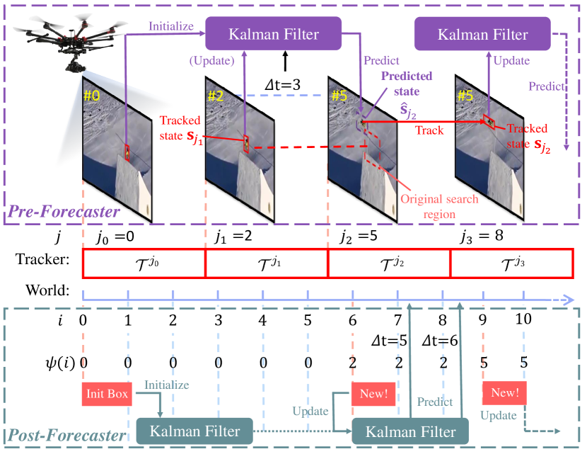
Figure 3: Visualization of the proposed predictive visual tracking framework. The red elements denote tracking procedure, the purple elements indicate pre-forecasting process, and the blue elements represent the post-forecaster.

Input: A video sequence of $T$ frames

          Init bounding box $\mathbf{b}_{\mathrm{g}}^{0}$ of the tracked object

Output: Paired estimated object bounding box $\hat{\mathbf{b}}^{i}_{\mathrm{r}}$ in all upcoming frames

1 Initialize world timestamp $t^{i}_{\mathrm{g}}$

2 Initialize the result box $\hat{\mathbf{b}}_{\mathrm{r}}^{0}=\mathbf{b}_{\mathrm{g}}^{0}$

3 for frame number $i=0$ to end do

4       if $i=0$ then

5             Tracker and forecasters initialization with $\mathbf{b}_{\mathrm{g}}^{0}$

6             Update $t^{0}_{\mathrm{r}}$ using Eq. (3)

7            

8      else

9             Find $j_{k}$ using Eq. (4)

10             if $j_{k}$ is new then

11                   Calculate $\Delta t_{k}=j_{k}-j_{k-1}$

12                   Predict $\hat{\mathbf{s}}_{j_{k}}$ with $\Delta t_{k}$ and $\mathbf{s}_{j_{k-1}}$ by Eq. (6)

13                   Correct search region with $\hat{\mathbf{s}}_{j_{k}}$

14                   Tracking in the corrected search region

15                   Update pre-forecaster with $\mathbf{s}_{j_{k}}$ by Eq. (8)

16                   $k++$

17                  

18            else

19                   Wait for the next new frame

20                  

21             end if

22            

23       end if

24      Find $\mathbf{b}_{\mathrm{r}}^{\psi(i)}$ using Eq. (5) (suppose $\psi(i)=j_{h}$)

25       if $\psi(i)>0$ then

26             Calculate $\Delta t_{\psi(i)}=i-\psi(i)$

27             if $\psi(i)$ is new then

28                   Calculate $\Delta t_{h}=j_{h}-j_{h-1}$

29                   Update post-forecaster with $\Delta t_{h}$ by Eq. (6) and Eq. (8)

30             end if

31            Predict $\hat{\mathbf{s}}_{i}$ using Eq. (9)

32             Obtain paired output box $\hat{\mathbf{b}}^{i}_{\mathrm{r}}=\mathbf{H}\hat{\mathbf{s}}_{i}$

33             Update tracker timestamp $t^{j_{k}}_{\mathrm{r}}$ using Eq. (3)

34            

35       end if

36      

37 end for

Algorithm 1 Predictive Visual Tracking

IV-B Post-Forecasting of Object States

As is illustrated in Sec. III-C, the latest input frame id $\psi(i)$ is smaller than the evaluated frame $i$. To compensate for the discrepancy between $\psi(i)$ and $i$, the post-forecaster basically follows the same work-flow of the pre-forecaster. Yet the update and prediction of KF in the post-forecaster are implemented asynchronously. Specifically, the prediction is carried out at each evaluation frame $i$, while the update is implemented only when $\psi(i)$ renovates. For a clear explanation, let’s suppose $\psi(i)=j_{h}$ below according to Eq. (5). For the prediction, the time interval $\Delta t_{\psi(i)}=i-\psi(i)$ is used to generate $\mathbf{F}(\Delta t_{\psi(i)})$ using Eq. (7). The predicted state $\hat{\mathbf{s}}_{i}$ and final output bounding box to be evaluated of frame $i$ is obtained using:

$$\hat{\mathbf{s}}_{i}=\mathbf{F}(\Delta t_{\psi(i)})\mathbf{s}_{j_{h}}~{},\hat{\mathbf{b}}^{i}_{\mathrm{r}}=\mathbf{H}\hat{\mathbf{s}}_{i}~{}.$$ (9)

When a new output $\mathbf{z}_{j_{h+1}}$ which corresponds to the input frame id $j_{h+1}$ becomes the latest processed frame, the time interval between 2 different raw output id $j_{h}$ and $j_{h+1}$ is $\Delta t_{h}=j_{h+1}-j_{h}$. With generated $\mathbf{F}(\Delta t_{h})$ and $\mathbf{Q}(\Delta t_{h})$ using Eq. (7), the post-forecaster adopts the same strategy to update as the pre-forecaster, i.e., Eq. (6) and Eq. (8), with different input id $j_{h}$ rather than $j_{k}$.

Remark 3: The speed of KF-based forecasters is about 500 FPS on a cheap CPU, and our prediction module is a generic framework which can be efficiently embedded into any tracker to improve the performance.

V Experiments

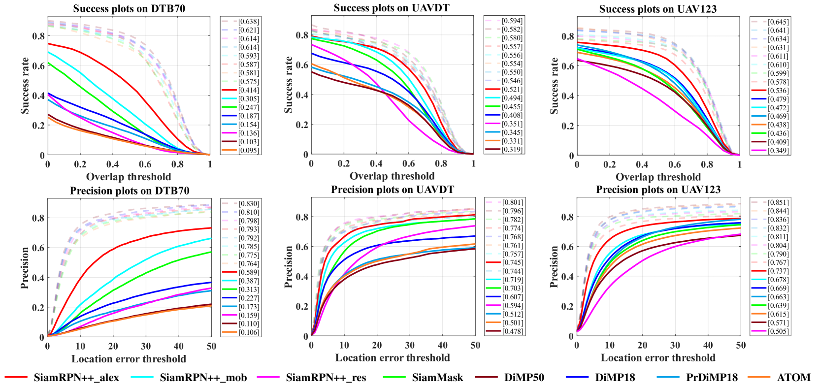
Figure 4: Performance of state-of-the-art trackers on the proposed LAE benchmark. The curves in solid colors report the performance of the 8 benchmarked trackers on LAE, whereas the dotted curves overlaid in semi-transparent same colors outline the performance obtained by the same trackers on the traditional offline benchmark. In brackets, we report the distance precision (DP) and area under curve (AUC) on LAE (in black) and on offline benchmark (in gray). Clearly, many offline promising trackers fail to maintain their robustness and accuracy in LAE benchmark.

TABLE II: Effect of the proposed PVT baseline on traditional SOTA trackers. The improvement in percentage and running speed are also reported for reference. ✓indecates whether the proposed 2 forecasters are enabled. Under most cases, the forecasters are able to boost the original performance of the SOTA trackers in new LAE benchmark.

Datasets	DTB70							UAVDT							UAV123
Metric	AUC			DP			FPS	AUC			DP			FPS	AUC			DP			FPS
Forecasters	✗	✓	$\Delta$(%)	✗	✓	$\Delta$(%)		✗	✓	$\Delta$(%)	✗	✓	$\Delta$(%)		✗	✓	$\Delta$(%)	✗	✓	$\Delta$(%)
SiamRPN++_res	0.136	0.201	+47.8	0.159	0.254	+59.7	6.0	0.351	0.467	+33.0	0.594	0.687	+15.7	6.0	0.349	0.434	+24.3	0.505	0.605	+19.8	5.6
SiamRPN++_mob	0.305	0.377	+23.6	0.387	0.518	+33.9	21.2	0.494	0.533	+7.9	0.719	0.74	+2.9	22.5	0.472	0.522	+10.6	0.678	0.722	+6.5	22.0
SiamMask	0.247	0.362	+46.6	0.313	0.504	+61.0	14.8	0.455	0.539	+18.5	0.703	0.751	+6.8	15.3	0.436	0.514	+17.9	0.639	0.701	+9.7	14.6

V-A Implementation Details

V-A1 Evaluation Platform

All the experimental evaluation in this work adopts NVIDIA Jetson AGX Xavier, a typical processing device onboard UAV.

V-A2 Evaluation Metric

This work adopts generally-used metrics in visual tracking for evaluation. The first is distance precision (DP) based on the center location error between the output box and the ground-truth box. The second is area under curve (AUC) represented by the intersection ratio of the predicted box and the ground-truth box.

Remark 4: Different from the offline benchmarks on which the tracking speed is separated from robustness, LAE actually considers the trade-off between efficiency and robustness of a tracker. A slow tracker may be extremely precise in offline benchmarks, while the large latency will make its performance drop significantly in LAE scenarios.

V-A3 Evaluation Datasets

We use three UAV tracking datasets for a comprehensive evaluation, i.e., DTB70 [12], UAVDT [33], and UAV123 [5] (all recorded at 30 FPS). Note that with the same datases, different benchmarks, i.e., offline latency-free benchmark and the proposed LAE benchmark are adopted while evaluation.

V-B Results on the LAE Benchmark

We employ eight SOTA trackers, i.e., SiamRPN++_res, SiamRPN++_mob, SiamRPN++_alex [9], SiamMask [13], ATOM [10], DiMP18, DiMP50 [11], and PrDiMP18 [14], to assess their performances in real-world tracking applications. Figure 4 exhibits the AUC and DP on traditional offline benchmark (curves in semi-transparent dash lines and values in gray) and the newly proposed LAE benchmark (curves in solid colors and values in black). In summary, all the SOTA trackers undergo a severe performance decline in LAE scenarios compared to the offline evaluation. For the fast trackers like SiamRPN++_alex [9], the performance drop caused by the latency is slightly smaller than the slow trackers like SiamRPN++_res [9]. For instance, in DTB70 [12], the DP of SiamRPN++_alex [9] is lowered by about 22.9% in LAE, while for SiamRPN++_res [9], the drop can be up to 76.7%. Such results have proven the importance of the tracking efficiency in the real-world latency-aware tracking. For DTB70 [12] with strong UAV motion, the trackers are faced with larger performance drop. Besides, the initialization time can also lead to non-negligible latency for the near-real-time trackers. Our LAE jointly assessing tracking accuracy and efficiency can provide a more realistic evaluation for the practical tracking applications.

V-C Predictive Visual Tracking Framework

V-C1 Overall Evaluation

The predictive framework is implemented on four SOTA trackers, i.e., SiamRPN++_res, SiamRPN++_mob, and SiamMask [13]. TABLE II presents the overall results on three datasets, where the DP, AUC, improvements in percentage, and running speed of the original trackers and predictive trackers are exhibited. In most cases, the predictive tracker can achieve far better results than its original framework with a gain of more than 20%. Besides, the slower the tracker runs, the larger improvements are achieved by the PVT framework. Take DTB70 [12] as an example, the PVT framework brings SiamRPN++_res [9] up by more than 40% in both DP and AUC. In terms of a faster tracker SiamRPN++_mob [9], the improvement is less remarkable (around 30%). Nevertheless, our PVT framework cannot work well on SiamRPN++_alex [9] with a real-time frame rate. The main reason is that the original tracker is fast enough to process each frame, so the original search region can be appropriately employed while the use of a pre-forecaster can be misleading.

Remark 5: Coupled with PVT, the non-real-time trackers can now achieve a comparable results than the real-time trackers lik eSiamRPN++_alex.

V-C2 Attribute-Based Evaluation

The performance under ten aerial tracking attributes (scale variation (SV), aspect ratio variation (ARV), occlusion (OCC), deformation (DEF), fast camera motion (FCM), in-plane rotation (IPR), out-of-plane rotation (OPR), out-of-view (OV), similar objects around (SOA), and motion blur (MB)) are reported in TABLE III. The proposed PVT has improved the robustness of the trackers notably, ranking the first in all attributes, e.g., in FCM, our tracker SimRPN++_mob_f outperforms its baseline by 57% and in the DEF scenario, our SiamMask_f nearly doubles its baseline. The attributes represent the typical challenges of the real-world UAV tracking compared with the general static object tracking, i.e., larger appearance variation and fast motion. In the LAE, the above difficulties are largely raised since some frames could be skipped. The attribute-based results have proven the promising effect of PVT in UAV tracking, alleviating the influence caused by the latency.

TABLE III: DP results in DTB70 [12] with LAE benchmark by UAV special attributes. Red denotes first place.

	ARV	DEF	FCM	IPR	MB	OCC	OPR	OV	SV	SOA
ATOM	0.116	0.070	0.079	0.101	0.060	0.140	0.071	0.076	0.114	0.091
DiMP18	0.214	0.158	0.197	0.22	0.153	0.256	0.135	0.236	0.287	0.210
DiMP50	0.127	0.083	0.082	0.111	0.055	0.155	0.077	0.236	0.124	0.112
PrDiMP18	0.154	0.150	0.136	0.142	0.100	0.197	0.136	0.071	0.210	0.146
SiamMask	0.247	0.246	0.241	0.236	0.167	0.361	0.128	0.222	0.287	0.34
SiamRPN++_mob	0.34	0.374	0.363	0.349	0.246	0.408	0.213	0.413	0.366	0.333
SiamRPN++_res	0.101	0.083	0.106	0.124	0.051	0.223	0.083	0.062	0.123	0.217
SiamMask_f (ours)	0.517	0.535	0.424	0.444	0.347	0.513	0.399	0.355	0.55	0.445
SiamRPN++_mob_f (ours)	0.427	0.429	0.572	0.482	0.483	0.409	0.219	0.498	0.501	0.436
SiamRPN++_res_f (ours)	0.227	0.241	0.181	0.206	0.087	0.286	0.133	0.18	0.203	0.295

V-C3 Ablation Study

To break down the performance gains from each part of PVT, ablation study is conducted on SiamRPN++_mob baseline [9]. As is shown in TABLE IV, each forecaster is embedded into the tracker individually. The results have illustrated that both forecasters can yield a performance gain on the original tracking framework (for the pre-forecaster, the improvement is about 11% and for the post-forecaster, it is around 20%). The final version equipped with both forecasters achieved the best result, up to 23.6% in AUC and 33.9% in DP.

TABLE IV: Ablation study of the 2 forecasters on SiamRPN++_mob [9]. ✓indicates whether the corresponding forecaster is enabled. Clearly, each forecaster can make an improvement and the final results with both forecasters are the best.

Tracker	Pre-Forecaster	Post-Forecaster	AUC	DP
Baseline			0.305	0.387
	✓		0.318	0.430
		✓	0.349	0.482
	✓	✓	0.377	0.518

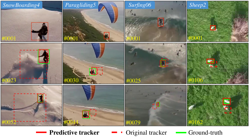
Figure 5: Visualization of representative latency-aware tracking scenes. The red boxes denotes bare tracker (dashed line) and proposed predictive tracker (solid line). The green boxes indicates ground truth. More latency-aware tracking sequences can be found at https://youtu.be/n8i8bREIFeM.

V-C4 Qualitative Evaluation

Figure 5 showed several tracking examples from DTB70 [12], adopting LAE benchmark. In the real-world latency-aware tracking, the bare trackers (in dashed red boxes) easily fall invalid, while the proposed PVT framework (in solid red boxes) has improved the robustness by a large margin.

VI Conclusions

We propose a brand-new task of predictive visual tracking along with a pioneering latency-aware evaluation (LAE) method for visual tracking community. The proposed LAE has formulated both accuracy and efficiency into a holistic evaluation process, to provide a realistic evaluation of the trackers for the robotics applications. Moreover, a generic and effective predictive tracking framework is proposed to compensate for the latency. The comprehensive experiments not only demonstrate the promising effect of our baseline approach, but also point out the demand to investigate latency-aware PVT for the robotics and computer vision community. We strongly believe our work can promote the applications of visual object tracking in the real world.

References

- [1] R. Bonatti, C. Ho, W. Wang, S. Choudhury, and S. Scherer, “Towards a Robust Aerial Cinematography Platform: Localizing and Tracking Moving Targets in Unstructured Environments,” in Proceedings of the IEEE/RSJ International Conference on Intelligent Robots and Systems (IROS), 2019, pp. 229–236.
- [2] C. Fu, A. Carrio, M. A. Olivares-Méndez, R. Suarez-Fernandez, and P. C. Cervera, “Robust Real-time Vision-Based Aircraft Tracking From Unmanned Aerial Vehicles,” in Proceedings of IEEE International Conference on Robotics and Automation (ICRA), 2014, pp. 5441–5446.
- [3] Y. Li, C. Fu, F. Ding, Z. Huang, and G. Lu, “AutoTrack: Towards High-Performance Visual Tracking for UAV with Automatic Spatio-Temporal Regularization,” in Proceedings of the IEEE Conference on Computer Vision and Pattern Recognition (CVPR), 2020, pp. 11 920–11 929.
- [4] Y. Wu, J. Lim, and M.-H. Yang, “Object Tracking Benchmark,” IEEE Transactions on Pattern Analysis and Machine Intelligence, vol. 37, pp. 1834–1848, 2015.
- [5] M. Mueller, N. Smith, and B. Ghanem, “A Benchmark and Simulator for UAV Tracking,” in Proceedings of European Conference on Computer Vision (ECCV), 2016, pp. 445–461.
- [6] H. Fan, L. Lin, F. Yang, P. Chu, G. Deng, S. Yu, H. Bai, Y. Xu, C. Liao, and H. Ling, “LaSOT: A High-Quality Benchmark for Large-Scale Single Object Tracking,” in Proceedings of the IEEE Conference on Computer Vision and Pattern Recognition (CVPR), 2019, pp. 5369–5378.
- [7] L. Huang, X. Zhao, and K. Huang, “GOT-10k: A Large High-Diversity Benchmark for Generic Object Tracking in the Wild,” IEEE Transactions on Pattern Analysis and Machine Intelligence, pp. 1–1, 2019.
- [8] B. Li, J. Yan, W. Wu, Z. Zhu, and X. Hu, “High Performance Visual Tracking with Siamese Region Proposal Network,” in Proceedings of the IEEE Conference on Computer Vision and Pattern Recognition (CVPR), 2018, pp. 8971–8980.
- [9] B. Li, W. Wu, Q. Wang, F. Zhang, J. Xing, and J. Yan, “SiamRPN++: Evolution of Siamese Visual Tracking With Very Deep Networks,” in Proceedings of the IEEE Conference on Computer Vision and Pattern Recognition (CVPR), 2019, pp. 4277–4286.
- [10] M. Danelljan, G. Bhat, F. Khan, and M. Felsberg, “ATOM: Accurate Tracking by Overlap Maximization,” in Proceedings of the IEEE Conference on Computer Vision and Pattern Recognition (CVPR), 2019, pp. 4655–4664.
- [11] G. Bhat, M. Danelljan, L. Gool, and R. Timofte, “Learning Discriminative Model Prediction for Tracking,” in Proceedings of the IEEE International Conference on Computer Vision (ICCV), 2019, pp. 6181–6190.
- [12] S. Li and D.-Y. Yeung, “Visual Object Tracking for Unmanned Aerial Vehicles: a Benchmark and New Motion Models,” in Proceedings of the AAAI Conference on Artificial Intelligence (AAAI), 2017.
- [13] Q. Wang, L. Zhang, L. Bertinetto, W. Hu, and P. H. S. Torr, “Fast Online Object Tracking and Segmentation: A Unifying Approach,” in Proceedings of IEEE Conference on Computer Vision and Pattern Recognition (CVPR), 2019, pp. 1328–1338.
- [14] M. Danelljan, L. Van Gool, and R. Timofte, “Probabilistic Regression for Visual Tracking,” in Proceedings of the IEEE Conference on Computer Vision and Pattern Recognition (CVPR), 2020, pp. 7181–7190.
- [15] J. F. Henriques, R. Caseiro, P. Martins, and J. Batista, “High-Speed Tracking with Kernelized Correlation Filters,” IEEE Transactions on Pattern Analysis and Machine Intelligence, vol. 37, no. 3, pp. 583–596, 2015.
- [16] H. K. Galoogahi, A. Fagg, and S. Lucey, “Learning Background-Aware Correlation Filters for Visual Tracking,” in Proceedings of IEEE International Conference on Computer Vision (ICCV), 2017, pp. 1144–1152.
- [17] M. Danelljan, G. Bhat, F. S. Khan, and M. Felsberg, “ECO: Efficient Convolution Operators for Tracking,” in 2017 IEEE Conference on Computer Vision and Pattern Recognition (CVPR), 2017, pp. 6931–6939.
- [18] M. Mueller, N. Smith, and B. Ghanem, “Context-Aware Correlation Filter Tracking,” in Proceedings of IEEE Conference on Computer Vision and Pattern Recognition (CVPR), 2017, pp. 1387–1395.
- [19] Z. Huang, C. Fu, Y. Li, F. Lin, and P. Lu, “Learning Aberrance Repressed Correlation Filters for Real-Time UAV Tracking,” in Proceedings of the IEEE International Conference on Computer Vision (ICCV), 2019, pp. 2891–2900.
- [20] Y. Li, C. Fu, F. Ding, Z. Huang, and J. Pan, “Augmented Memory for Correlation Filters in Real-Time UAV Tracking,” in Proceedings of the IEEE/RSJ International Conference on Intelligent Robots and Systems (IROS), 2020, pp. 1559–1566.
- [21] Y. Li, C. Fu, Z. Huang, Y. Zhang, and J. Pan, “Keyfilter-Aware Real-Time UAV Object Tracking,” in Proceedings of the IEEE International Conference on Robotics and Automation (ICRA), 2020, pp. 193–199.
- [22] F. Li, C. Fu, F. Lin, Y. Li, and P. Lu, “Training-Set Distillation for Real-Time UAV Object Tracking,” in Proceedings of the IEEE International Conference on Robotics and Automation (ICRA), 2020, pp. 9715–9721.
- [23] Y. He, C. Fu, F. Lin, Y. Li, and P. Lu, “Towards Robust Visual Tracking for Unmanned Aerial Vehicle with Tri-Attentional Correlation Filters,” in Proceedings of the IEEE/RSJ International Conference on Intelligent Robots and Systems (IROS), 2020, pp. 1575–1582.
- [24] C. Fu, F. Ding, Y. Li, J. Jin, and C. Feng, “Dr2track: Towards real-time visual tracking for uav via distractor repressed dynamic regression,” in Proceedings of the IEEE/RSJ International Conference on Intelligent Robots and Systems (IROS), 2020, pp. 1597–1604.
- [25] M. Müller, A. Bibi, S. Giancola, S. Al-Subaihi, and B. Ghanem, “TrackingNet: A Large-Scale Dataset and Benchmark for Object Tracking in the Wild,” in Proceedings of the European Conference on Computer Vision (ECCV), 2018, pp. 300–317.
- [26] Q. Liu, Z. He, X. Li, and Y. Zheng, “PTB-TIR: A Thermal Infrared Pedestrian Tracking Benchmark,” IEEE Transactions on Multimedia, vol. 22, pp. 666–675, 2020.
- [27] A. Lukezic, U. Kart, J. Käpylä, A. Durmush, J. Kämäräinen, J. Matas, and M. Kristan, “CDTB: A Color and Depth Visual Object Tracking Dataset and Benchmark,” in Proceedings of the IEEE/CVF International Conference on Computer Vision (ICCV), 2019, pp. 10 012–10 021.
- [28] M. Dunnhofer, A. Furnari, G. Farinella, and C. Micheloni, “Is First Person Vision Challenging for Object Tracking? The TREK-100 Benchmark Dataset,” ArXiv, vol. abs/2011.12263, 2020.
- [29] B. Li, C. Fu, F. Ding, J. Ye, and F. Lin, “All-Day Object Tracking for Unmanned Aerial Vehicle,” arXiv preprint arXiv:2101.08446, 2021.
- [30] M. Kristan, A. Leonardis, J. Matas, M. Felsberg, R. Pflugfelder, L. C. Zajc, et al., “The Visual Object Tracking VOT2017 Challenge Results,” in Proceedings of the IEEE International Conference on Computer Vision Workshops (ICCVW), 2017, pp. 1949–1972.
- [31] M. Kristan, A. Leonardis, J. Matas, M. Felsberg, R. Pflugfelder, L. C. Zajc, T. Vojír, et al., “The Sixth Visual Object Tracking VOT2018 Challenge Results,” in Proceedings of the European Conference on Computer Vision (ECCV) Workshops, 2018.
- [32] M. Kristan, J. Matas, A. Leonardis, M. Felsberg, R. Pflugfelder, Joni-Kristian, et al., “The Seventh Visual Object Tracking VOT2019 Challenge Results,” in Proceedings of the IEEE/CVF International Conference on Computer Vision Workshop (ICCVW), 2019, pp. 2206–2241.
- [33] D. Du, Y. Qi, H. Yu, Y. Yang, K. Duan, G. Li, W. Zhang, Q. Huang, and Q. Tian, “The unmanned aerial vehicle benchmark: object detection and tracking,” in Proceedings of the European Conference on Computer Vision (ECCV), 2018, Conference Proceedings, pp. 370–386.
- [34] N. Wang, W. Zhou, Y. Song, C. Ma, and H. Li, “Real-Time Correlation Tracking Via Joint Model Compression and Transfer,” IEEE Transactions on Image Processing, vol. 29, pp. 6123–6135, 2020.
- [35] A. G. Howard, M. Zhu, B. Chen, D. Kalenichenko, W. Wang, T. Weyand, M. Andreetto, and H. Adam, “Mobilenets: Efficient Convolutional Neural Networks for Mobile Vision Applications,” arXiv preprint arXiv:1704.04861, 2017.
- [36] M. Sandler, A. Howard, M. Zhu, A. Zhmoginov, and L.-C. Chen, “Mobilenetv2: Inverted Residuals and Linear Bottlenecks,” in Proceedings of the IEEE Conference on Computer Vision and Pattern Recognition (CVPR), 2018, pp. 4510–4520.
- [37] M. Li, Y.-X. Wang, and D. Ramanan, “Towards Streaming Perception,” in Proceedings of the European Conference on Computer Vision (ECCV), 2020, pp. 473–488.
- [38] R. E. Kalman, “A New Approach to Linear Filtering and Prediction Problems,” Transactions of the ASME-Joural of Basic Engineering, pp. 35–45, 1960.