Rapidly-exploring Random Forest: Adaptively Exploits Local Structure with Generalised Multi-Trees Motion Planning

Abstract

Sampling-based motion planners perform exceptionally well in robotic applications that operate in high-dimensional space. However, most works often constrain the planning workspace rooted at some fixed locations, do not adaptively reason on strategy in narrow passages, and ignore valuable local structure information. In this paper, we propose Rapidly-exploring Random Forest (rrf^*)—a generalised multi-trees motion planner that combines the rapid exploring property of tree-based methods and adaptively learns to deploys a Bayesian local sampling strategy in regions that are deemed to be bottlenecks. Local sampling exploits the local-connectivity of spaces via Markov Chain random sampling, which is updated sequentially with a Bayesian proposal distribution to learns the local structure from past observations. The trees selection problem is formulated as a multi-armed bandit problem, which efficiently allocates resources on the most promising tree to accelerate planning runtime. rrf^* learns the region that is difficult to perform tree extensions and adaptively deploys local sampling in those regions to maximise the benefit of exploiting local structure. We provide rigorous proofs of completeness and optimal convergence guarantees, and we experimentally demonstrate that the effectiveness of rrf^*’s adaptive multi-trees approach allows it to performs well in a wide range of problems.

I Introduction

Motion planning is one of the fundamental methods for robots to navigate and integrate with the real-world. Obstacles and physical constraints are ubiquitous regardless of the type of robotic applications, and we wish to safely and efficiently navigate the robot from some initial state to a target state. Sampling-based motion planners (SBPs) are of a class of robust methods to perform motion planning. SBPs do no need to explicitly construct the often intractable high-dimensional Configuration Space (C-space). SBP samples C-space randomly for valid connections and iteratively builds a roadmap of connectivity. SBPs are guaranteed to find a solution if one exists [1]. Further developments on SBPs had granted asymptotic optimality [2]—a guarantee that the solution will converge, in the limit, to the optimal solution.

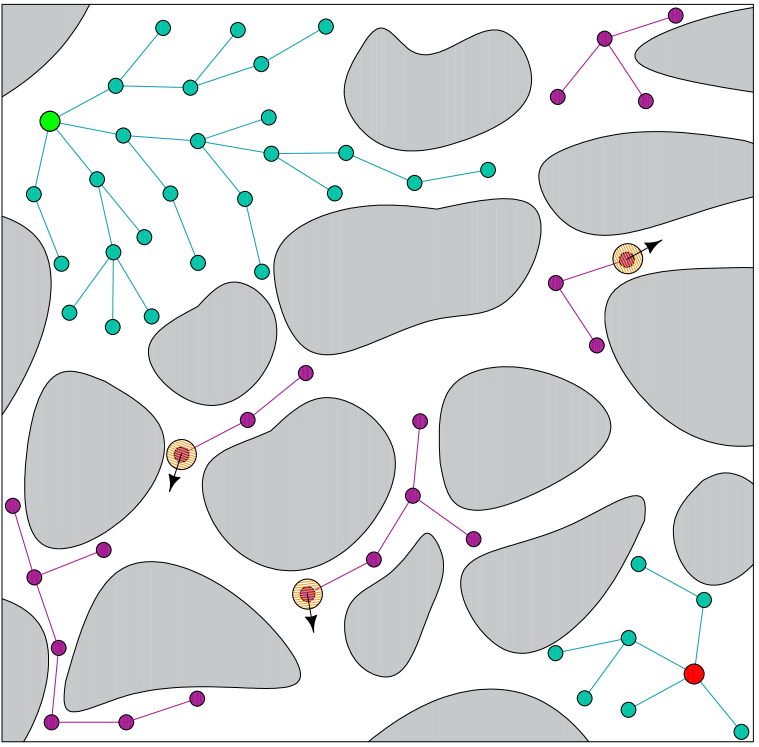
Figure 1: Overview illustration of rrf^* using multiple trees to adaptively plans on the current most promising tree, which rapidly explores visible space and exploits local structures with Bayesian local sampling. Green and red nodes refers to the initial $q_{\text{init}}$ and target $q_{\text{target}}$ configuration; teal and purple trees are the rooted $T_{\text{init}},T_{\text{target}}$ and local trees respectively. Orange hatched circles are the current states of local samplers sampling for their respective local trees. rrf^* learns to creates new local trees in highly constrained regions that are hard to extend from root trees, of which will be benefited from proposing informed samples through Bayesian local sampling.

One of the fundamental issues with SBPs lies in SBP’s approach—the exceedingly low likelihood of sampling within narrow passages. Intuitively, regions with low visibility will have a low probability to be randomly sampled. Therefore, when SBPs perform roadmap-based planning by random sampling and creating connections in C-space, highly constrained regions become problematic as they limit the connectivity of free space [3, 4]. Narrow passages severely restrict the performance of SBPs because SBPs throw away the unlikely samples that do fall within narrow passages if the tree failed to expand. Consequently, narrow passages will bottleneck the tree’s growth until a series of tree expansions had successfully created connections within the restricting narrow passages.

Our contribution is an incremental multi-trees SBP—Rapidly-exploring Random Forest (rrf^*)—that learns from sampling information and adjust planning strategy accordingly. We formulate rrf^* to learns regions that are likely to be bottlenecked and adaptively deploys Bayesian local sampling to exploits C-space’s local structure. Unlike previous local SBPs that deploy local trees everywhere regardless of the nearby region’s complexity, rrf^* utilises the rapid growth of the rooted trees approach for open spaces and adaptively uses local trees within bottlenecks. Bayesian local sampling tackles the narrow passage problem by performing sequential Markov chain Monte Carlo (MCMC) random walks within the passage, and at the same time, updates its proposal distribution from sampled outcomes. In additions, rrf^* plans with multiple trees and allocates planning resources on the most promising tree by the reward signal from our multi-armed bandit formulation. We provide rigorous proofs on completeness and optimal convergence guarantees. Experimentally, we show that rrf^* achieves superior results in a wide range of scenarios, especially, rrf^* yields high sample efficiency in highly constrained C-space.

II Related Work

One of the most influential works on SBPs is Probabilistic Roadmap (prm), which creates a random roadmap of connectivity that can be reused [5]. Rapidly-exploring Random Tree (rrt) [6] follows a similar idea but instead uses a tree structure to obtain a more rapid single-query solution. Most SBPs minimises some cost, e.g., distance metric or control cost. Therefore, prm^∗ [7] and rrt^* [8] are introduced that exhibit asymptotic optimal guarantee. The runtime performance of SBPs had been one of the main focus in existing works. For example, to address the narrow passage problem, some planners focus the random sampling to specific regions in C-space [9]. Such an approach often requires some technique to discover narrow passages, e.g., using bridge test [10], space projection [11], heuristic measures of obstacles boundary [12, 13], and densely samples at discovered narrow regions [14, 15, 16]. There are also sampling techniques that improve sampling efficiency by using a restricted or learned sampling distribution [17, 18, 19, 20], which either formulate some regions for generating samples or deploy a machine learning approach to learn from experience. However, while those approaches improved sampling efficiency, they do not directly address the limited visibility issue within narrow passages.

Some planners had employed a multi-tree approach to explore C-space more efficiently. For example, growing bidirectional trees can speed up the exploration process because tree extensions at different origin are subject to a different degree of difficulty [21]. Potential tree locations can be searched with the bridge test, followed by a learning technique to model the probability of tree selection [22]. Local trees had been employed for growing multiple trees in parallel [23, 4]. However, current approaches utilise local trees regardless of the complexity of the nearby regions. While those approaches had improved sampling efficiency, it would be more beneficial to deploy local planners dependent on the C-space complexity adaptively. Several SBPs had utilised Markov Chain Monte Carlo (MCMC) for local planning, as it allows utilisation of information observed from previous samples [24]. Monte Carlo random walk planner searches free space by constructing a Markov Chain to propose spaces with high contributions [25]. The roadmap of a PRM can be formulated as the result of simultaneously running a set of MCMC explorations [26]. Therefore, the connectives between feasible states can be modelled as a chain of samples walking within the free space. Our proposing rrf^* exploits this property by utilising a Bayesian approach in proposing chained samples by sequentially updating our belief on the space that are deemed to be bottlenecks.

III Rapidly-exploring Random Forest

Motion planning’s objective is to construct a feasible trajectory from an initial configuration $q_{\text{init}}$ to a target configuration $q_{\text{target}}$, where $q\in C\subseteq\mathbb{R}^{d}$ denotes a state the C-space and $d\geq 2$ is the dimensionality. The obstacle spaces $C_{\text{obs}}$ denotes the set of invalid states, and the set of free space $C_{\text{free}}$ is defined as the closure set $\text{cl}(C\setminus C_{\text{obs}})$. In motion planning, there is often some cost function that the planner wants to optimise.

Problem 1 (Asymptotic optimal planning)

Given $C$, $C_{\text{obs}}$, a pair of initial $q_{\text{init}}$ and target $q_{\text{target}}$ configurations, a cost function $\mathcal{L}_{c}\colon\sigma\to[0,\infty)$, and let $\Gamma(C_{\text{free}})$ denotes the set of all possible trajectories in $\text{cl}(C_{\text{free}})$. Find a solution trajectory $\sigma^{*}$ that exhibits the minimal cost. That is, find $\sigma^{*}$ such that $\sigma^{*}(0)=q_{\text{init}}$, $\sigma^{*}(1)=q_{\text{target}}$, and $\mathcal{L}_{c}(\sigma^{*})=\min_{\sigma\in\Gamma(C_{\text{free}})}\mathcal{L}_{c}(\sigma)$.

III-A High-level description

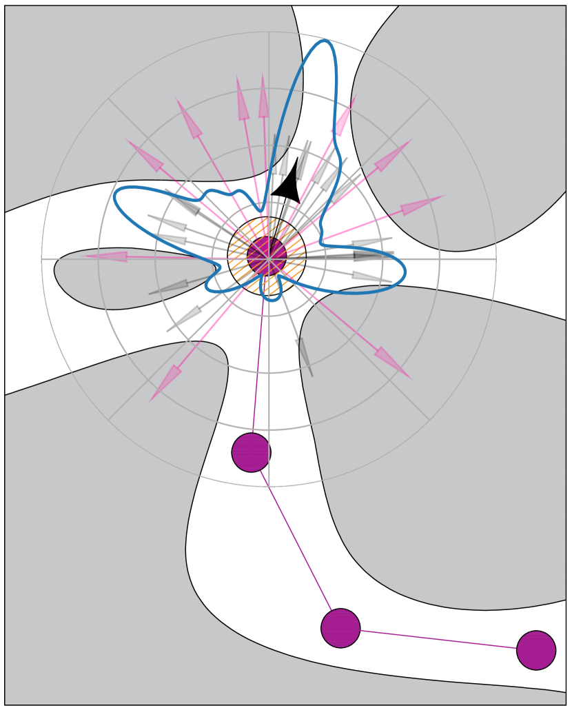
Figure 2: Illustration of rrf^* performing Bayesian local sampling for a local tree. The spherical proposal distribution is overlaid on the local sampler as a blue curve, which is sequentially learned after 10 previous failed samples (purple arrows). The transparent grey arrows illustrates the likelihood of sampling 20 times from the probability distribution shown.

rrf^* uses multiple trees to adaptively explores and exploits different regions of C-space. Traditional approaches use only a single tree rooted at $q_{\text{initial}}$ to construct a roadmap of connected configurations. The tree grows outwards by sampling random configurations that create a new connection to the closest node. Since the tree expansion is limited to a local scope bounded by the neighbourhood visibility of the frontier tree nodes, such an approach will often reject updates from valid samples when there exists no free route from the closest existing node towards the sampled configuration. rrf^* overcomes this limitation by addressing the sampling-based motion planning problem with a divide-and-conquer approach. rrf^* follows the approach in [27] which uses local trees for Bayesian local sampling. However, instead of purely using Markov Chain to plan within C-space [27], rrf^* adaptively locates difficult regions for tree extensions and only proposes new local trees when local planning is beneficial. rrf^* uses two rooted trees and reformulate the spawning of local-trees as an adaptive selection process. Previous work replaces the motion planning problem entirely with Markov Chains; however, we argue that the most effective approach relies on deploying the most appropriate strategy in specific regions. As a result, rrf^* is biased more on exploration in regions that contain lots of free space, whereas in restricted bottlenecks, rrf^* will adaptively deploy local sampling within narrow passages.

rrf^* formulates the tree-selection problem as a multi-armed bandit (MAB) problem. Using a MAB approach helps develop an adaptive selection strategy that actively selects the tree that is more promising in tree extensions. MAB allows rrf^* to focus its resources on trees that are more likely to successfully expand and switch to the local sampling approach when it is more profitable.

III-B Learning Local Sampling with Bayesian Updates

We model the local sampling procedure as a Markovian process. A local planner’s state $\Theta_{t}$ refers to its spatial location and $C_{\text{obs}}$ nearby at step $t$. It cannot be directly observed, but we can observe the outcome by sampling a direction $x_{\text{new}}$ from the local planner’s current location $q_{t}$ at $t$ and use $x_{\text{new}}$ to extends towards a nearby configuration $q_{\text{new}}$. The observation outcome is said to be successful if $\sigma_{\mathchoice{\vbox{\halign{#\cr\rightarrowfill@{\scriptstyle}\crcr\nointerlineskip\cr$\hfil\displaystyle q_{n}q_{\text{new}}\hfil$\crcr}}}{\vbox{\halign{#\cr\rightarrowfill@{\scriptstyle}\crcr\nointerlineskip\cr$\hfil\textstyle q_{n}q_{\text{new}}\hfil$\crcr}}}{\vbox{\halign{#\cr\rightarrowfill@{\scriptscriptstyle}\crcr\nointerlineskip\cr$\hfil\scriptstyle q_{n}q_{\text{new}}\hfil$\crcr}}}{\vbox{\halign{#\cr\rightarrowfill@{\scriptscriptstyle}\crcr\nointerlineskip\cr$\hfil\scriptscriptstyle q_{n}q_{\text{new}}\hfil$\crcr}}}}\in C_{\text{free}}$, where the notation $\sigma_{\mathchoice{\vbox{\halign{#\cr\rightarrowfill@{\scriptstyle}\crcr\nointerlineskip\cr$\hfil\displaystyle q_{i}q_{j}\hfil$\crcr}}}{\vbox{\halign{#\cr\rightarrowfill@{\scriptstyle}\crcr\nointerlineskip\cr$\hfil\textstyle q_{i}q_{j}\hfil$\crcr}}}{\vbox{\halign{#\cr\rightarrowfill@{\scriptscriptstyle}\crcr\nointerlineskip\cr$\hfil\scriptstyle q_{i}q_{j}\hfil$\crcr}}}{\vbox{\halign{#\cr\rightarrowfill@{\scriptscriptstyle}\crcr\nointerlineskip\cr$\hfil\scriptscriptstyle q_{i}q_{j}\hfil$\crcr}}}}$ denote the connection between the configurations $q_{i}$ and $q_{j}$. We use a Bayesian approach in our work to sequentially update and improve our proposal distribution based on the observed outcomes.

When a local sampler at state $\Theta_{t}$ is expanding a local tree via Bayesian local sampling, it draws a direction $x_{t,i}$ from a proposal distribution $\mathcal{Q}_{t}$ and extend towards $x_{t,i}$, where $i$ denotes the $i$^th attempt to extends the connection. If it is unsuccessful, the local planner remains at state $\Theta_{t}$, and another sample is drawn from the updated proposal distribution $x_{t,i+1}\sim\mathcal{Q}_{t}(x\>|\>x_{t-1},\mathcal{X}_{i+1})$, where $x_{t-1}$ is the previous successful direction and $\mathcal{X}_{i+1}$ is the set of all previously failed directions at iteration $i+1$. Whereas if the extension towards $x_{t,i}$, we say that $x_{t}:=x_{t,i}$ (the successful direction at $t$), and local planner will transits to state $\Theta_{t+1}$ and proceed to draws sample from $x_{t+1,1}\sim\mathcal{Q}_{t+1}(x\>|\>x_{t},\mathcal{X}_{1})$ in the next iteration, where $\mathcal{X}_{1}:=\emptyset$. Therefore, the update follows the Bayesian updating scheme where $f_{\text{posterior}}\propto f_{\text{prior}}\cdot f_{\text{likelihood}}$ and subsequently uses current posterior as the next prior.

rrf^* uses the von-Mises Fisher distribution [28] $f(\boldsymbol{x}\>|\>\boldsymbol{\mu},\kappa)$ as the initial prior $f_{\text{prior}}$ with $\boldsymbol{\mu}$ being the previous successful direction. After observing the sampling outcome, we use a likelihood function to reduce the probability to sample again in the previously failed directions. The likelihood function is formulated as $f_{\text{likelihood}}(x\>|\>x^{\prime})\propto\big{(}1-k(x,x^{\prime})\big{)}$, where $k$ is the kernel function to incorproate failure information from $\mathcal{X}$. We can write the posterior of the proposal distribution for local sampler at state $\Theta_{t}$ as

$$\mathcal{Q}_{t}(x\>|\>x_{t-1},\mathcal{X}_{i}) =\frac{\mathcal{Q}_{t}(x\>|\>x_{t-1},\mathcal{X}_{i-1})\left(1-\beta\cdot k(x,x^{\prime}_{i-1})\right)}{\alpha_{i}},$$ (1)

where $x^{\prime}_{i-1}\in\mathcal{X}_{i}=\set{x^{\prime}_{1},\ldots x^{\prime}_{i-1}}$ for $i>1$, $\beta$ is a scalar that controls the influence of the kernel, and $\alpha_{i}$ is the normalising factor. Note that $\mathcal{Q}_{i}(x\>|\>x_{i-1},\mathcal{X}_{1})$ reduces to $f_{\text{prior}}(x\>|\>x_{i-1})$ as $\mathcal{X}_{1}:=\emptyset$. We use the periodic squared exponential [29] to sequentially incorporate past sampled results into $\mathcal{Q}$, given by $k(x,x^{\prime})=\sigma^{2}\exp({-{2\sin^{2}(\pi(x-x^{\prime})/p)}/{\lambda^{2}}}),$ where $\lambda$ is the length scale, $\sigma$ is a scaling factor, and $p=2\pi$ is the period of repetition. Fig. 2 illustrates an example of the sequentially updated distribution $\mathcal{Q}$ after 10 failed samples.

III-C Maximising Successes with Multi-Armed Bandit

The tree selections process is formulated as a MAB problem to maximise resource allocation. Each tree $T_{i}\in\mathcal{T}$ is located at some configuration in $C_{\text{free}}$, which exhibits varying degree of complexity dependent on its surroundings. Hence, there are often some trees in $\mathcal{T}$ that exhibit a higher success tree expansion rates than others. Using MAB scheduler helps to bias the exploration of the trees rooted at $q_{\text{init}}$ and $q_{\text{target}}$ when there are abundant free spaces (usually results in a faster initial solution), or rrf^* can create local trees for local-connectivity exploitation when C-space is highly restricted (helps to plan within narrow passages). Because spaces with complex surroundings (narrow passages) can utilise local-connectivity information to exploits obstacles’ structure (as discussed in section III-B); whilst areas with high visibility allow us to allocate more resources on rapid exploring.

We formalise the tree selections in rrf^* as a Mortal MAB [30] with non-stationary reward sequences [31]. Each arm $a_{i}\in A$ is a stateful local sampler that transverse within $C_{\text{free}}$, with state at time $t$ denoted as $a_{i,t}$ that consists of the spatial location, previous successful direction and the number of failed expansions. At each $t$ it samples $C$ to makes an observation $o_{t}$ and receives a reward $R(a_{i,t})$. We consider discrete time and Bernoulli arms, with arms success probability at time $t$ formulated as

$$\forall{i\in\{1,...,k\}}\colon\mathbb{P}(a_{i,t}\mid a_{i,t-1},o_{t-1}).$$ (2)

We consider the arms as independent random variables with $\mathbb{P}(a_{i,t})$ having non-stationary distribution dependent on its previous samples. The reward $R(a_{i,t})$ is a functional mappings of the current state of the local sampler to a real value reward, where

$$R(a_{i,t})=\begin{cases}1&\text{if $a_{i,t}$ located in $C_{\text{free}}$}\\ 0&\text{otherwise}.\end{cases}$$ (3)

The reward sequence $R(a_{i,1}),\ldots,R(a_{i,t})$ is a stochastic sequence with unknown payoff distributions and can changes rapidly according to the complexity of C-space. Each arm has a stochastic lifetime after which they would expire due to events such as running into a dead-end or stuck in a narrow passage. In practice we prune away an arm $a_{i}$ if it is deemed unprofitable when its success probability $\mathbb{P}(a_{i,t}\mid a_{i,t-1},o_{t-1})$ is lower than some threshold $\eta$. The action space to create new local trees is infinite, but we identify high potential areas to spawn new arms through learning areas in $C_{\text{free}}$ that exhibit frequent failed tree-extension attempts.

III-D Implementation

Input: $q_{\text{init}},q_{\text{target}},N,k,\epsilon,\eta$

Initialise: $\mathcal{T}\leftarrow\{\;T_{\text{init}}(V=\{q_{\text{init}}\},E=\emptyset),\,T_{\text{target}}(V=\{q_{\text{target}}\},E=\emptyset)\;\}$; $A\leftarrow$ Initialise arms; $n\leftarrow 1$;

1 while $n\leq N$ do

2      

3      $\mathcal{T},A\leftarrow\texttt{ProposeLocalTree}(\mathcal{T},A,k,\epsilon)$

4       $T_{i},a_{i}\leftarrow\texttt{PickTreeMAB}(\mathcal{T},A)$

5      

6      if $T_{i}\in\set{T_{\text{init}},T_{\text{target}}}$ then

7             $q_{\text{rand}}\leftarrow$ SampleFree

8             $q_{\text{closest}}\leftarrow$ closest node in $T_{i}$

9             $q_{\text{new}}\leftarrow$ $q_{\text{closest}}$ with $\epsilon$ step towards $q_{\text{rand}}$

10            

11       else

12             $q_{\text{closest}}\leftarrow$ current location of local sampler in $T_{i}$

13             $q_{\text{new}}\leftarrow$ samples for $T_{i}$ locally via MCMC

14            

15      if $\sigma_{\mathchoice{\vbox{\halign{#\cr\rightarrowfill@{\scriptstyle}\crcr\nointerlineskip\cr$\hfil\displaystyle q_{\text{closest}}\;q_{\text{new}}\hfil$\crcr}}}{\vbox{\halign{#\cr\rightarrowfill@{\scriptstyle}\crcr\nointerlineskip\cr$\hfil\textstyle q_{\text{closest}}\;q_{\text{new}}\hfil$\crcr}}}{\vbox{\halign{#\cr\rightarrowfill@{\scriptscriptstyle}\crcr\nointerlineskip\cr$\hfil\scriptstyle q_{\text{closest}}\;q_{\text{new}}\hfil$\crcr}}}{\vbox{\halign{#\cr\rightarrowfill@{\scriptscriptstyle}\crcr\nointerlineskip\cr$\hfil\scriptscriptstyle q_{\text{closest}}\;q_{\text{new}}\hfil$\crcr}}}}\in C_{\text{free}}$ then

16             Join $q_{\text{new}}$ to all $T_{i}\in\mathcal{T}$ within $\epsilon$-distance

17             if $q_{\text{new}}$ joined to $T_{\text{init}}$ then Rewire($T_{\text{init}}$)

18             Update location of $a_{i}$ to $q_{\text{new}}$

19             $n\leftarrow n+1$

20            

21      Updates $T_{i},a_{i}$ probability

      

       $\triangleright$ Remove local tree with low prob

22       if $T_{i}\not\in\{T_{\text{init}},T_{\text{target}}\}$ and $\mathbb{P}(a_{i})<\eta$ then

23             $A\leftarrow A\setminus\{a_{i}\}$

24            

25      

Algorithm 1 rrf^* Algorithm

Algorithm 1 illustrates the overall flow of the rrf^* algorithm. The planner begins by initialising two trees rooted at $q_{\text{init}}$ and $q_{\text{target}}$, similar to Bidirectional RRT [21]. Then, arms are initialised into $A$, which stores the trees’ success probability, and subsequently used in the PickTreeMAB multi-armed bandit subroutine in Alg. 1. rrf^* explores C-space by picking $a_{i}\in A$ and its corresponding $T_{i}\in\mathcal{T}$ based on how likely it is for the $T_{i}$ tree extension to be successful. Am arm $a_{i}$ is drawn from a multinomial distribution with each $a_{i}\in A$ having probability formulated by eq. 2. Then, if $T_{i}$ is a tree rooted at either $q_{\text{init}}$ or $q_{\text{target}}$ (Alg. 1), the standard tree-based planning procedure is followed—a random free configuration $q_{\text{rand}}$ is uniformly and randomly sampled with SampleFree, followed by searching for the closest node in $T_{i}$ and attempting to extend the node towards $q_{\text{rand}}$ by an $\epsilon$ distance. On the other hand, if $T_{i}$ is a local tree we utilise local sampling to exploit local structure (Alg. 1). Local sampling incorporates past successes by utilising a Bayesian sequential updates procedure (section III-B), which uses a MCMC random walker that constructs a chained sampling with the sequentially learned proposal distribution $\mathcal{Q}$ in eq. 1 to propose $q_{\text{new}}$. In both cases, if the connection from $q_{\text{closest}}$ to $q_{\text{new}}$ is valid then the connection will be added to $T_{i}$ accordingly. Whenever we add a new node to $T_{i}$, we search its nearby $\epsilon$ radius for nodes from other trees and merges both trees (Alg. 1). This procedure naturally combines trees as part of the tree expansions process, which gradually reduces the number of local trees as the roadmap fills $C_{\text{free}}$. If a new node or tree is joined to the root tree $T_{\text{init}}$, the standard rewire procedure is performed to guarantees asymptotic optimality (see [7] for details on Rewire). Finally, rrf^* updates the arm $a_{i}$’s success probability and will discard the local sampler if its probability is lower than some threshold $\eta$, e.g., when the local sampler is stuck in some dead-end. The tree $T_{i}$ will remain to be in $\mathcal{T}$ for future connections, but the arm $a_{i}$ will be discarded such that there will be no local sampler actively performing local sampling for $T_{i}$.

Algorithm 2 shows the subroutine to propose new local tree locations. Local trees are only created when a constrained location with high potential are proposed in Alg. 2, where $p_{\text{potential}}$ denotes the probability that the proposing location will be benefited from local sampling. Numerous different techniques can be used for this proposal procedure. For example, (i) location’s proposal can be supplied by the user, (ii) by laying prior and using Bayesian optimisation to sequentially update the posterior, or (iii) directly learned by neural networks through past experiences. In our experiments, we implemented a simple cluster-based technique that is quick to compute. The location proposer identifies regions that have a considerable amount of samples $q_{\text{rand}}\in C_{\text{free}}$ that repeatedly failed to connect to existing trees and propose those regions based on the failure density. Our approach utilises sample information that is readily available without extra effort, which results in a non-trivial performance gain. The location proposer does not need to be perfect, but proposing regions near narrow passages will significantly enhance the effectiveness of exploiting local structures.

IV Analysis

In this section, we analyse the behaviour of the rrf^* algorithm and its algorithmic tractability. In additions, we provide proof of completeness and optimality guarantee.

IV-1 Tractability of Planning with Local Trees

Although rrf^* creates new local trees to explore narrow passages, tractability is retained as the number of local trees is bounded.

Assumption 1

The free space $C_{\text{free}}\subseteq C$ is a finite set.

Theorem 1 (Termination of creating new local trees)

Let Assumption 1 hold. Then, the accumulative number of local trees $n_{\text{local-tree}}$ for any given C-space is always finite. That is, there exists a constant $\varphi\in\mathbb{Z},\varphi\geq 0$ such that $n_{\text{local-tree}}\leq\varphi$ for any given $C$.

Proof:

From Alg. 2, if there exists other $T_{i}\in\mathcal{T}$ within $\epsilon$ distance (Alg. 2), the proposing configuration will be joined to the existing local tree $T_{i}$ and no new tree will be created (Alg. 2). Hence, every new local tree $T_{j}$ must be at least $\epsilon$-distance away from $T_{i}\in\mathcal{T}$ where $T_{i}\neq T_{j}$. We can formulate each node in $T_{i}\in\mathcal{T}$ as a $d$-dimensional volume hypersphere with $\epsilon$ radius centred at the node. In the limiting case, $C_{\text{free}}$ will be completely filled by the volume of $\epsilon$-balls. Let $\epsilon(q)$ denotes the $\epsilon$-ball of $q$, and $V_{t}$ be the set of all nodes from all trees $T\in\mathcal{T}$ at iteration $t$. Then, the above statement is formally stated as $\lim_{t\to\infty}C_{\text{free}}\setminus\bigcup_{q\in V_{t}}\epsilon(q)=\emptyset.$ Therefore, $n_{\text{local-tree}}$ is upper bounded by the number of $\epsilon$-balls that fully fills $C_{\text{free}}$. It is immediate that if $C_{\text{free}}$ is a finite set, $n_{\text{local-tree}}$ will always be bounded by a constant. ∎

1 function $\textnormal{{ProposeLocalTree}}(\mathcal{T},A,k,\epsilon)$

2       if $|A|<k$ then

3             $q_{\text{local}},p_{\text{potential}}\leftarrow$ Propose new local tree location

4             if $p_{\text{potential}}>\delta_{\text{threshold}}$ then

5                   Join $q_{\text{local}}$ to all $T\in\mathcal{T}$ within $\epsilon$-distance

6                   if Not joined to existing tree then

7                         $T\leftarrow G(V=\{q_{\text{local}}\},E=\emptyset)$

8                         $\mathcal{T}\leftarrow\mathcal{T}\cup\{T\}$

9                         $A\leftarrow$ Add new local sampler $a$ to $A$

10                        

11                  

12            

      return $\mathcal{T},A$

        $\triangleright$ new local tree is added

13      

Algorithm 2 Propose new local tree

IV-2 Joining of Local Trees

Local trees that are connectable are guaranteed to be eventually connected.

Theorem 2 (see [22])

Let $C_{\text{free}}^{\prime}\subseteq C_{\text{free}}$ be a connected free space. Select $k$ configurations $q_{1},...,q_{k}$ randomly from $C_{\text{free}}^{\prime}$ including $q_{\text{init}}$ and $q_{\text{target}}$. Set $q_{1},...,q_{k}$ as root nodes and extend $k$ trees from these points. Let $n$ be the total number of nodes that all these trees extended, and $\gamma\in\mathbb{R}$ be a real number in $(0,1]$. If $n$ satisfies

$$\begin{split}n\geq\,&k(\alpha\beta\epsilon)^{-1}\ln[4(1-\epsilon)]\ln\{3\ln[2k^{2}(1-\epsilon)]/\gamma\beta\}\\ &+k\mu(C_{\text{free}})/\mu(C)\ln(3k^{2}/2\gamma)\end{split}$$ (4)

then the probability that each pair of these $k$ trees can be attached successfully is at least $1-\gamma$.

Proof:

Due to space constrains, see [22] for full proof. ∎

Theorem 3 (Joining of local trees)

Let $T_{i},T_{j}\in\mathcal{T}$ be instances of local trees in $C_{\text{free}}^{\prime}$ where $T_{i}\neq T_{j}$. If there exists a feasible trajectory to connect $T_{i}$ to $T_{j}$, it is guaranteed that both trees will joined as a single tree as $t\to\infty$.

Proof:

Theorem 1 states that the number of local trees is finite. Hence, in the limiting case, all local trees satisfy the real-valued bound given by Theorem 2. ∎

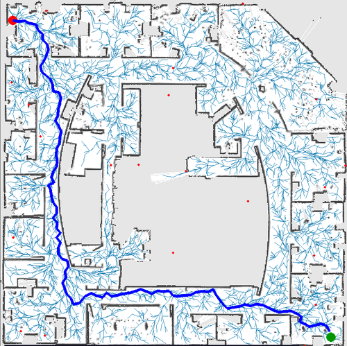
(a) Intel lab

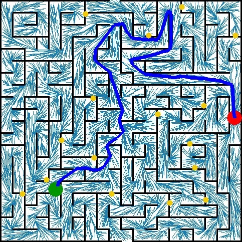
(b) Maze

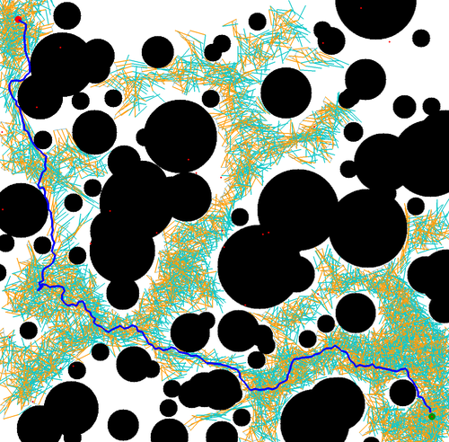
(c) 4D rover arm

(d) 6D manipulator

Figure 3: Environments. (3(a)) Intel lab map data and with a point mass robot as baseline. (3(b)) Cluttered maze environment with extremely limited visibility. (3(c)) Rover arm with two spatial dimensionality and two rotational joints. (3(d)) Manipulator with six rotational joints for an object pickup task.

IV-3 Probabilistic Completeness

rrf^* attains probabilistic completeness as its number of uniform random samples approaches infinity.

Theorem 4 (Infinite random sampling)

Let $n_{i,t}$ denotes the number of uniformly random configurations used for creating new node in rrf^* at time $t$. The number $n_{i,t}$ always increases without bound, i.e., as $t\to\infty$, $n_{i,t}\to\infty$.

Proof:

As stated in theorem 1, as $t\to\infty$ there will be no new local trees being created. Therefore, the behaviour of rrf^* sampling will be dominated by Alg. 1 Alg. 1 to Alg. 1 when all local trees in $\mathcal{T}$ are joined to $T_{\text{init}}$. Therefore, rrf^* will be reduced to use SampleFree to samples uniformly in $C_{\text{free}}$. ∎

Theorem 5

Let $n^{\textsc{rrf}\textsuperscript{*}}_{t}$ and $n^{\textsc{rrt}\textsuperscript{*}}_{t}$ be the number of uniformly random configurations sampled at time $t$ for rrf^* and rrt^* respectively. There exists a constant $\phi\in\mathbb{R}$ such that $\lim_{t\to\infty}\mathbb{E}[n^{\textsc{rrf}\textsuperscript{*}}_{t}/n^{\textsc{rrt}\textsuperscript{*}}_{t}]\leq\phi.$

Proof:

There exist two different sampling schemes being employed in rrf^*. The (i) uniform random sampling in Alg. 1 Alg. 1, and (ii) exploitative local sampling in Alg. 1. The total number of exploitative local sampling $n_{\text{local-samp}}$ by MCMC in (ii) is the summation of each local sampler’s sampled configurations $n_{\text{local-samp}}=\sum_{i=1}^{|\mathcal{T}|}n_{i,t}$. Deriving from Theorem 1, since the number of local trees in the lifetime of rrf^* is bounded by a constant, the number of local sampling $n_{\text{local-samp}}$ will also be bounded by a constant. On the other hand, Theorem 4 states that the number of uniformly sampled configurations in (i) is unbounded and approaches infinity. Therefore, the ratio of the total number of uniformly random configurations between rrf^* and rrt^* will be bounded by at most a constant as the behaviour of rrf^* will converge to rrt^* as $t\to\infty$. ∎

With Theorems 4 and 5, the probabilistic completeness of rrf^* is immediate.

Theorem 6 (Probabilistic Completeness)

rrf^* inherits the same probabilistic completeness of rrt^*, i.e., $\lim_{i\to\infty}\mathbb{P}(\{\sigma(i)\cap q_{\text{target}}\neq\emptyset\})=1$.

IV-4 Asymptotic optimality planning

Theorem 7 (Asymptotic optimality)

Let $\sigma^{*}_{t}$ be rrf^*’s solution at time $t$, and $c^{*}$ be the minimal cost for problem 1. If a solution exists, then the cost of $\sigma^{*}_{t}$ will converge to the optimal cost almost-surely. That is, $\mathbb{P}\left(\left\{\lim_{t\to\infty}c(\sigma^{*}_{t})=c^{*}\right\}\right)=1.$

Proof:

From Theorem 3, all local trees in the same $C_{\text{free}}^{\prime}$ will converge to a single tree. According to Theorem 4 there will be infinite sampling available to improve that tree. Together with adequate rewiring procedure at Alg. 1 Alg. 1 (see [7]), it is guaranteed that the solution will converge to the optimal solution as $t\to\infty$. ∎

V Experimental Results

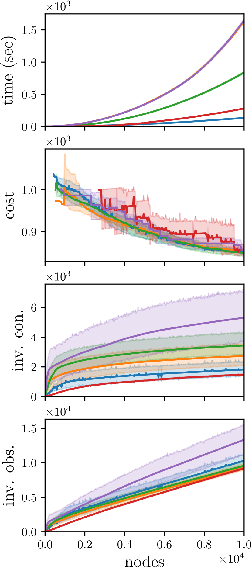
(a) Intel lab

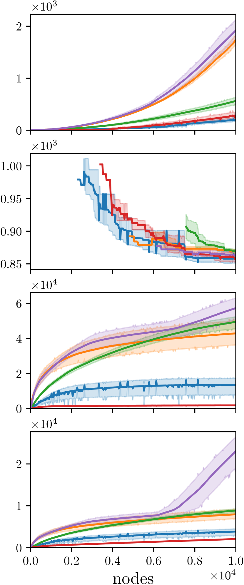
(b) Maze

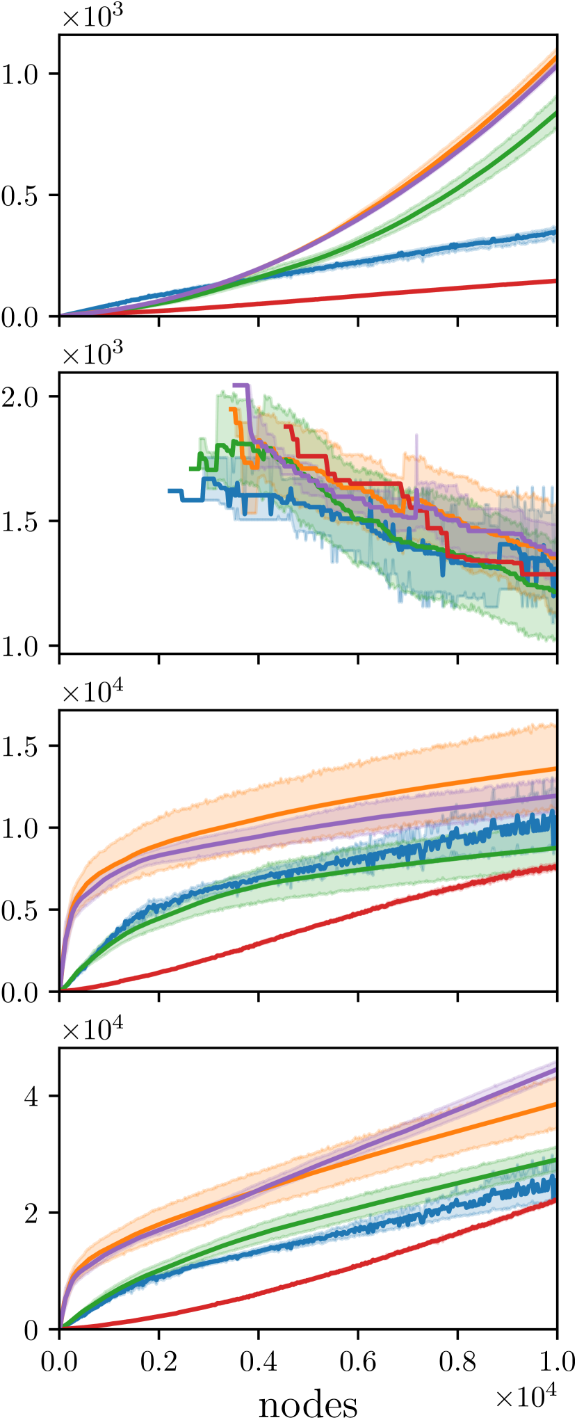
(c) Rover arm

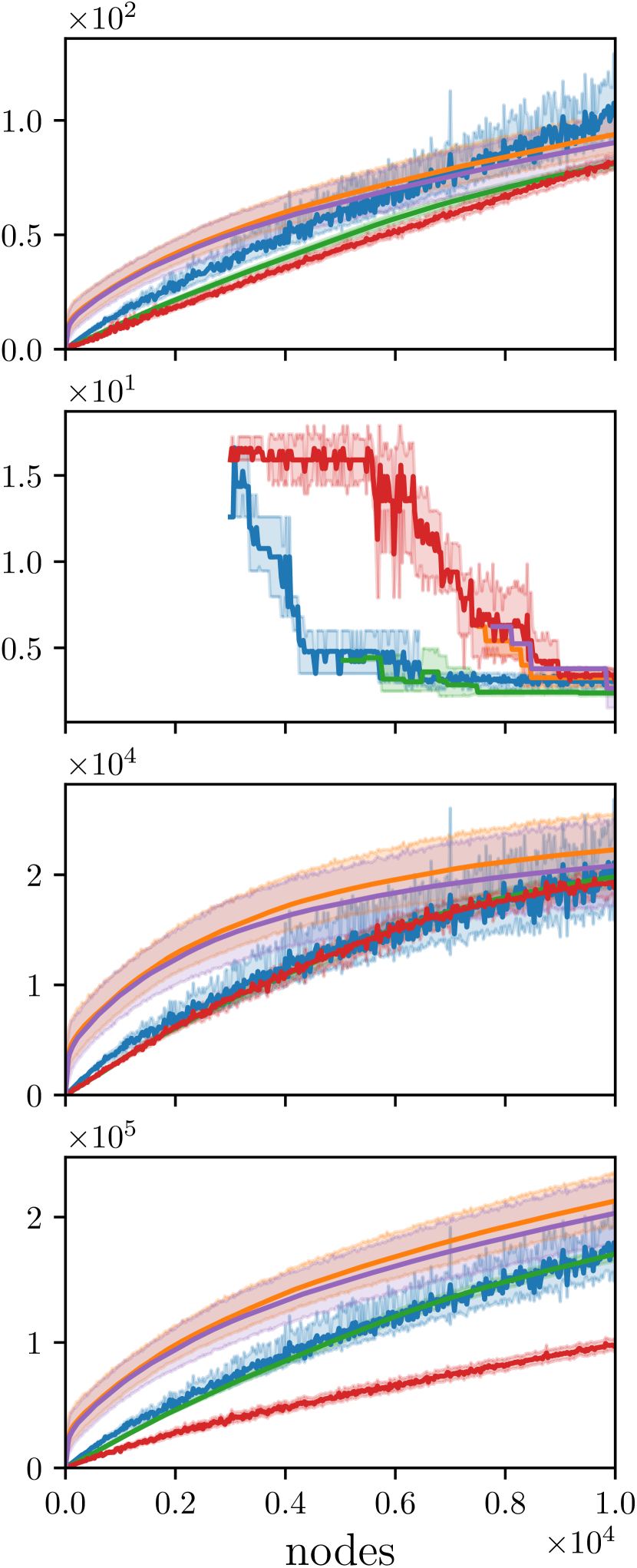
(d) Manipulator

Figure 4: Top to bottom are time (seconds), cost, invalid connections and invalid obstacles against number of nodes. Each experiment is repeated 10 times, with each solid line and shaded region representing the mean and $95\%$ confidence interval. Invalid obstacles and invalid connections refers to the number of invalid samples due to $q_{\text{rand}}\in C_{\text{obs}}$ or intermediate collision, respectively. For the cost metric, the line appears at the first instance that a solution is found.

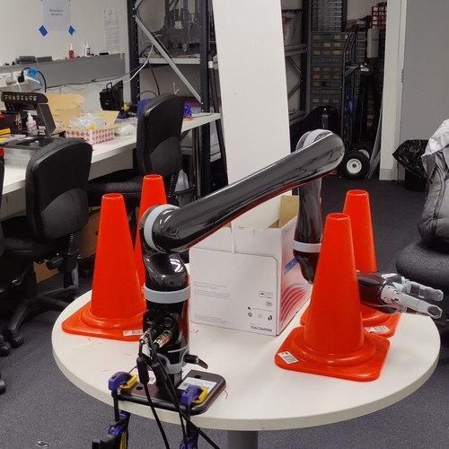
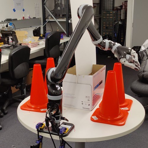
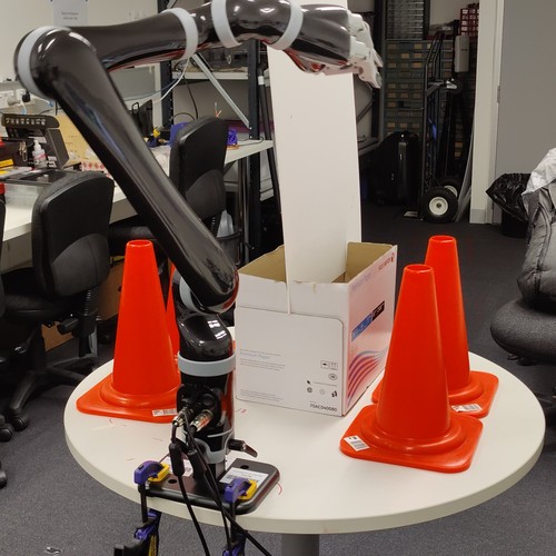
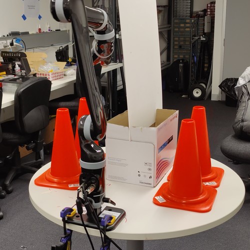
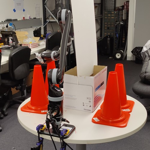
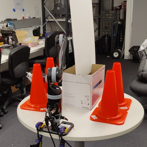
(a) Sequence of trajectory executed by JACO arm

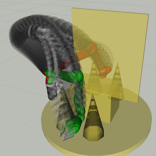
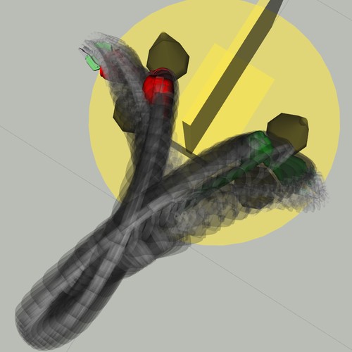
(b) Trajectory trail

Figure 5: Evaluation of rrf^*’s algorithmic robustness on a JACO robotic arm. (5(a)) Sequence of trajectory execution in a cluttered environment. (5(b)) Solution trajectory trail after planning with a time budget of five seconds.

We evaluate the performance of rrf^* in various environments with a range of degree of complexity, as shown in Fig. 3. Intel lab and maze are with a point mass robot in $\mathbb{R}^{2}$ to plan a trajectory from some initial configuration to a target configuration. Rover’s arm also has a two-dimensional spatial location, but with two additional rotational joints that denote the rotational angles of the robot arm. The rover arm needs to navigate while rotating its arm to avoid collisions. Manipulator environment is a 6 dof TX90 robotic manipulator that operates in a 3D cluttered environment; with a task to move the manipulator between two cupboards while holding a cup. The environment contains many structures that restrict the manipulator’s movement. Qualitatively, we evaluate rrf^*’s algorithmic robustness by testing the resulting trajectory in a real-world JACO arm (Fig. 5). In terms of environment complexity, maze (Fig. 3(b)) and manipulator (Fig. 3(d)) are highly cluttered due to the limited visibility and abundance of narrow passages; whereas the other two environments contain more free space with multiple homotopy classes of solution trajectories.

rrf^* is evaluated against rrt^* [7], bi-rrt^∗ [21], rrdt^∗ [4], and Informed rrt^* [17], implemented under the same planning framework in Python. Overall, rrf^* performs consistently across all environments regardless of its complexity. rrf^*’s performance is similar to rrdt^∗ because both methods are using multiple local trees to explore C-space. However, rrf^* adaptively creates new local trees only in regions deemed bottlenecks and coupled with a MAB selection that balances choosing rooted trees or local trees that are promising. Therefore, similar to bi-rrt^∗ it inherits the benefit of obtaining fast solution in open areas (e.g. see cost metric in Figs. 4(a) and 4(c)), and similar to rrdt^∗ it obtains fast solution in cluttered areas (see cost in Figs. 4(b) and 4(d)). The runtime savings of rrf^* comes from the reduced number of collision checks by reducing invalid samples. Since both rrf^* and rrdt^∗ uses multiple trees to explore C-space, their metric of invalid connections and invalid obstacles (bottom two rows of Fig. 4) are often the lowest among all others. However, unlike rrdt^∗, rrf^* is adaptive to the current workspace with a heuristic to only deploy local trees in highly constrained (section III-D). Therefore, the performance of rrf^* can be seen as a hybrid between traditional motion planner and multi-trees planner; the same reason allows rrf^* to quickly converges its solution when compared to rrdt^∗ (cost in Fig. 4(d)).

VI Conclusion

We present rrf^*, a generalised adaptive multi-tree approach for asymptotic optimal motion planning. rrf^* uses multiple local trees to adaptively utilise a beneficial local sampling strategy when constrained regions are discovered. Bayesian local sampling in a cluttered area allows rrf^* to exploit local structures and effectively tackle narrow passages. rrf^* adaptively deploys local sampling in restricted regions when necessary, which overcome the issue of multi-trees approach having slow initial time in open spaces.

References

- [1] Lydia E. Kavraki, Mihail N. Kolountzakis and J.-C. Latombe “Analysis of Probabilistic Roadmaps for Path Planning” In Proceedings of IEEE International Conference on Robotics and Automation, 1996 DOI: 10/d66p3t
- [2] Mohamed Elbanhawi and Milan Simic “Sampling-Based Robot Motion Planning: A Review” In IEEE Access 2, 2014, pp. 56–77 DOI: 10/gdkx6g
- [3] David Hsu et al. “On Finding Narrow Passages with Probabilistic Roadmap Planners” In Robotics: The Algorithmic Perspective: 1998 Workshop on the Algorithmic Foundations of Robotics, 1998
- [4] Tin Lai, Fabio Ramos and Gilad Francis “Balancing Global Exploration and Local-Connectivity Exploitation with Rapidly-Exploring Random Disjointed-Trees” In Proceedings of The International Conference on Robotics and Automation, 2019
- [5] Lydia E. Kavraki, Petr Svestka, J.. Latombe and Mark H. Overmars “Probabilistic Roadmaps for Path Planning in High-Dimensional Configuration Spaces” In IEEE Trans. Robot. Autom. 12.4, 1996, pp. 566–580 DOI: 10/fsgth3
- [6] Steven M. LaValle “Rapidly-Exploring Random Trees: A New Tool for Path Planning” In TR 98-11 Comput. Sci. Dept Iowa State Univ., 1998
- [7] S. Karaman and E. Frazzoli “Incremental Sampling-Based Algorithms for Optimal Motion Planning” In Proceedings of Robotics: Science and Systems, 2010 DOI: 10.15607/RSS.2010.VI.034
- [8] Sertac Karaman and Emilio Frazzoli “Sampling-Based Algorithms for Optimal Motion Planning” In Int. J. Robot. Res. 30.7, 2011, pp. 846–894 DOI: 10/c2wgw5
- [9] Anna Yershova, Léonard Jaillet, Thierry Siméon and Steven M. LaValle “Dynamic-Domain RRTs: Efficient Exploration by Controlling the Sampling Domain” In Proceedings of IEEE International Conference on Robotics and Automation, 2005
- [10] Steven A. Wilmarth, Nancy M. Amato and Peter F. Stiller “MAPRM: A Probabilistic Roadmap Planner with Sampling on the Medial Axis of the Free Space” In Proceedings of IEEE International Conference on Robotics and Automation, 1999
- [11] Andreas Orthey and Marc Toussaint “Rapidly-Exploring Quotient-Space Trees: Motion Planning Using Sequential Simplifications”, 2019 arXiv: http://arxiv.org/abs/1906.01350
- [12] Liangjun Zhang and Dinesh Manocha “An Efficient Retraction-Based RRT Planner” In Proceedings of IEEE International Conference on Robotics and Automation, 2008
- [13] Junghwan Lee, OSung Kwon, Liangjun Zhang and Sung-eui Yoon “SR-RRT: Selective Retraction-Based RRT Planner” In Proceedings of IEEE International Conference on Robotics and Automation, 2012
- [14] David Hsu, Tingting Jiang, John Reif and Zheng Sun “The Bridge Test for Sampling Narrow Passages with Probabilistic Roadmap Planners” In Proceedings of IEEE International Conference on Robotics and Automation, 2003
- [15] Zheng Sun, D. Hsu, Tingting Jiang and H. Kurniawati “Narrow Passage Sampling for Probabilistic Roadmap Planning” In IEEE Trans. Robot. 21.6, 2005, pp. 1105–1115 DOI: 10/bh6v9h
- [16] Wei Wang, Xin Xu, Yan Li and Jinze Song “Triple RRTs: An Effective Method for Path Planning in Narrow Passages” In Adv. Robot. 24.7, 2010, pp. 943 DOI: 10/fv9c9p
- [17] Jonathan D. Gammell, Timothy D. Barfoot and Siddhartha S. Srinivasa “Informed Sampling for Asymptotically Optimal Path Planning” In IEEE Trans. Robot. 34.4, 2018, pp. 966–984 DOI: 10/gd5sp3
- [18] Tin Lai and Fabio Ramos “Learning to Plan Optimally with Flow-Based Motion Planner”, 2020 arXiv: http://arxiv.org/abs/2010.11323
- [19] Brian Ichter, James Harrison and Marco Pavone “Learning Sampling Distributions for Robot Motion Planning” In 2018 IEEE International Conference on Robotics and Automation (ICRA), 2018 DOI: 10/gf7t7z
- [20] Guillaume Sartoretti et al. “PRIMAL: Pathfinding via Reinforcement and Imitation Multi-Agent Learning” In IEEE Robot. Autom. Lett. 4.3 IEEE, 2019, pp. 2378–2385 DOI: 10/ggzj7h
- [21] James J. Kuffner and Steven M. LaValle “RRT-Connect: An Efficient Approach to Single-Query Path Planning” In Proceedings of IEEE International Conference on Robotics and Automation, 2000
- [22] Wei Wang, Lei Zuo and Xin Xu “A Learning-Based Multi-RRT Approach for Robot Path Planning in Narrow Passages” In J. Intell. Robot. Syst. 90.1-2, 2018, pp. 81–100 DOI: 10/gc7cqd
- [23] Morten Strandberg “Augmenting RRT-Planners with Local Trees” In Proceedings of IEEE International Conference on Robotics and Automation, 2004
- [24] Weifeng Chen “Motion Planning with Monte Carlo Random Walks”, 2015
- [25] Hootan Nakhost, Jörg Hoffmann and Martin Müller “Resource-Constrained Planning: A Monte Carlo Random Walk Approach.” In International Conference on Automated Planning and Scheduling (ICAP), 2012
- [26] Ibrahim Al-Bluwi, Thierry Siméon and Juan Cortés “Motion Planning Algorithms for Molecular Simulations: A Survey” In Comput. Sci. Rev. 6.4, 2012, pp. 125–143 DOI: 10/gdkx6f
- [27] Tin Lai, Philippe Morere, Fabio Ramos and Gilad Francis “Bayesian Local Sampling-Based Planning” In IEEE Robot. Autom. Lett. 5.2 IEEE, 2020, pp. 1954–1961 DOI: 10/gg2n24
- [28] Nicholas I. Fisher “Statistical Analysis of Circular Data” Cambridge University Press, 1995
- [29] David JC MacKay “Introduction to Gaussian Processes” In NATO ASI Ser. F Comput. Syst. Sci. 168, 1998, pp. 133–166
- [30] Deepayan Chakrabarti, Ravi Kumar, Filip Radlinski and Eli Upfal “Mortal Multi-Armed Bandits” In Advances in Neural Information Processing Systems, 2009
- [31] Omar Besbes, Yonatan Gur and Assaf Zeevi “Stochastic Multi-Armed-Bandit Problem with Non-Stationary Rewards” In Advances in Neural Information Processing Systems, 2014