An Amazing Prime Heuristic

1. Introduction

The record for the largest known twin prime is constantly changing. For example, in October of 2000, David Underbakke found the record primes:

$$83475759\cdot 2^{64955}\pm 1.$$

The very next day Giovanni La Barbera found the new record primes:

$$1693965\cdot 2^{66443}\pm 1.$$

The fact that the size of these records are close is no coincidence! Before we seek a record like this, we usually try to estimate how long the search might take, and use this information to determine our search parameters. To do this we need to know how common twin primes are.

It has been conjectured that the number of twin primes less than or equal to $N$ is asymptotic to

$$2C_{2}\int_{2}^{N}\frac{dx}{(\log x)^{2}}\sim\frac{2C_{2}N}{(\log N)^{2}}$$

where $C_{2}$, called the twin prime constant, is approximately $0.6601618$. Using this we can estimate how many numbers we will need to try before we find a prime. In the case of Underbakke and La Barbera, they were both using the same sieving software (NewPGen by Paul Jobling) and the same primality proving software (Proth.exe by Yves Gallot) on similar hardware–so of course they choose similar ranges to search. But where does this conjecture come from?

In this chapter we will discuss a general method to form conjectures similar to the twin prime conjecture above. We will then apply it to a number of different forms of primes such as Sophie Germain primes, primes in arithmetic progressions, primorial primes and even the Goldbach conjecture. In each case we will compute the relevant constants (e.g., the twin prime constant), then compare the conjectures to the results of computer searches. A few of these results are new–but our main goal is to illustrate an important technique in heuristic prime number theory and apply it in a consistent way to a wide variety of problems.

1.1. The key heuristic

A heuristic is an educated guess. We often use them to give a rough idea of how long a program might run–to estimate how long we might need to wait in the brush before a large prime comes wandering by. The key to all the results in this chapter is the following:

The prime number theorem states that the number of primes less than $n$ is asymptotic to $1/\log n$. So if we choose a random integer $m$ from the interval $[1,n]$, then the probability that $m$ is prime is asymptotic to $1/\log n$.

Let us begin by applting this to a few simple examples.

First, as $n$ increases, $1/\log n$ decreases, so it seemed reasonable to Hardy and Littlewood to conjecture that there are more primes in the set $\{1,2,3,\ldots,k\}$ than in $\{n+1,n+2,n+3,\ldots,n+k\}$. In other words, Hardy and Littlewood [21] conjectured.

Conjecture 1.1.

For sufficiently large integers $n$, $\pi(k)\geq\pi(n+k)-\pi(n)$.

They made this conjecture on the basis of very little numerical evidence saying “An examination of the primes less than 200 suggests forcibly that $\rho(x)\leq\pi(x)(x\geq 2)$” (page 54). (Here $\rho(x)=\limsup_{n\rightarrow\infty}\pi(n+x)-\pi(x)$.) By 1961 Schinzel [37] had verified this to $k=146$ and by 1974 Selfridge et. al. [19] had verified it to 500. As reasonable sounding as this conjecture is, we will give a strong argument against it in just a moment.

Second, suppose the Fermat numbers $F_{n}=2^{2^{n}}+1$ behaved as random numbers. Then the probability that $F_{n}$ is prime should be about $1/\log(F_{n})\sim 1/(2^{n}\log 2)$. So the expected number of such primes would be on the order of $\sum_{n=0}^{\infty}1/(2^{n}\log 2)=2/\log 2$. This is the argument Hardy and Wright used when they presented the following conjecture [22, pp. 15, 19]:

Conjecture 1.2.

There are finitely many Fermat primes.

The same argument, when applied to the Mersenne numbers, Woodall numbers, or Cullen numbers suggest that there are infinitely many primes of each of these forms. But it would also imply there are infinitely many primes of the form $3^{n}-1$, even though all but one of these are composite. So we must be a more careful than just adding up the terms $1/\log n$. We will illustrate how this might be done in the case of polynomials in the next section.

As a final example we point out that in 1904, Dickson conjectured the following:

Conjecture 1.3.

Suppose $a_{i}$ and $b_{i}$ are integers with $a_{i}>1$. If there is no prime which divides each of

$$\{b_{1}x+a_{1},b_{2}x+a_{2},\ldots,b_{n}x+a_{n}\}$$

for every $x$, then there are infinitely many integers values of $x$ for which these terms are simultaneously prime.

How do we arrive at this conclusion? By our heuristic, for each $x$ the number $b_{i}x+a_{i}$ should be prime with a probability $1/\log N$. If the probabilities that each term is prime are independent, then the whole set should be prime with probability $1/(\log N)^{n}$. They are not likely to be independent, so we expect something on the order of $C/(\log N)^{n}$ for some constant $C$ (a function of the coefficients $a_{i}$ and $b_{i}$).

In the following section we will sharpen Dickson’s conjecture in to a precise form like that of the twin prime conjecture above.

1.2. A warning about heuristics

What (if any) value do such estimates have?

They may have a great deal of value for those searching for records and predicting computer run times, but mathematically they have very little value. They are just (educated) guesses, not proven statements, so not “real mathematics.” Hardy and Littlewood wrote: “Probability is not a notion of pure mathematics, but of philosophy or physics” [21, pg 37 footnote 4]. They even felt it necessary to apologize for their heuristic work:

Here we are unable (with or without Hypothesis $R$) to offer anything approaching a rigorous proof. What our method yields is a formula, and one which seems to stand the test of comparison with the facts. In this concluding section we propose to state a number of further formulae of the same kind. Our apology for doing so must be (1) that no similar formulae have been suggested before, and that the process by which they are deduced has at least a certain algebraic interest, and (2) that it seems to us very desirable that (in default of proof) the formula should be checked, and that we hope that some of the many mathematicians interested in the computative side of the theory of numbers may find them worthy of their attention. ([21, pg 40])

When commenting on this Bach and Shallit wrote:

Clearly, no one can mistake these probabilistic arguments for rigorous mathematics and remain in a state of grace. Nevertheless, they are useful in making educated guesses as to how number-theoretic functions should “behave.” ([2, p. 248])

Why this negative attitude? Mathematics seeks proof. It requires results without doubt or dependence on unnecessary assumptions. And to be blunt, sometimes heuristics fail! Not only that, they sometimes fail for even the most cautious of users. In fact we have already given an example (perhaps you noticed?)

Hardy and Littlewood, like Dickson, conjectured that if there is no prime which divides each of the following terms for every $x$, then they are simultaneously primes infinitely often:

$$\{x+a_{1},x+a_{2},x+a_{3},x+a_{4},x+a_{5},\ldots,x+a_{k}\}$$

[21, Conjecture X]. This is a special case of Dickson’s Conjecture is sometimes called the prime $k$-tuple conjecture. We have also seen that they conjectured $\pi(k)\geq\pi(n+k)-\pi(n)$ (conjecture 1.1). But in 1972, Douglas Hensley and Ian Richards proved that one of these two conjectures is false [24, 25, 35]!

Perhaps the easiest way to see the conflict between these conjectures is to consider the following set of polynomials found by Tony Forbes [16]:

$$\{n-p_{24049},n-p_{24043},\ldots,n-p_{1223},n-p_{1217},$$

$$n+p_{1217},n+p_{1223},\ldots,n+p_{24043},n+p_{24049}\}$$

where $p_{n}$ is the $n$-th prime. By Hardy and Littlewood’s first conjecture there are infinitely many integers $n$ so that each of these $4954$ terms are prime. But the width of this interval is just $48098$ and $\pi(48098)<4954$. So this contradicts the second conjecture.

If one of these conjectures is wrong, which is it? Most mathematicians feel it is the second conjecture that $\pi(k)\geq\pi(n+k)-\pi(n)$ which is wrong. The prime $k$-tuple conjecture receives wide support (and use!) Hensley and Richards predicted however

Now we come to the second problem mentioned at the beginning of this section: namely the smallest number $x_{1}+y_{1}$ for which $\pi(x_{1}+y_{1})>\pi(x_{1})+\pi(y_{1})$. We suspect, even assuming the $k$-tuples hypothesis (B) is eventually proved constructively, that the value of $x_{1}+y_{1}$ will never be found; and moreover that no pair $x,y$ satisfying $\pi(x+y)>\pi(x)+\pi(y)$ will ever be computed. ([19, p. 385])

What can we conclude from this example of clashing conjectures? First that heuristics should be applied only with care. Next they should then be carefully tested. Even after great care and testing you should not stake to much on their predictions, so read this chapter with the usual bargain hunter’s mottoes in mind: “buyer beware” and “your mileage may vary.”

1.3. Read the masters

The great mathematician Abel once wrote ”It appears to me that if one wants to make progress in mathematics, one should study the masters and not the pupils.” Good advice, but this is an area short of masters.

Hardy and Littlewood’s third paper on their circle method [21] is one of the first key papers in this area. In this paper they made the first real step toward the proving the Goldbach conjecture, then gave more than a dozen conjectures on the distribution of primes. Their method is far more complicated than what we present here–but it laid the basis for actual proofs of some related results.

The approach we take here may have first been laid out by Cherwell and Wright [11, section 3] (building on earlier work by Cherwell [10], Stäckel [43], and of course Hardy and Littlewood). The same approach was taken by Bateman and Horn [3] (see also [4]).

Many authors give similar arguments including Brent, Shanks [40, 42, 41] and P’olya [32].

There are also a couple excellent “students” we should mention. Ribenboim included an entire chapter on heuristics in his text “the new book of prime number records” [34]. Riesel also develops much of this material in his fine book [36]. See also Schroeder [39, 38].

And as enthusiastic students we also add our little mark. Again, most of what we present here was first done by others. Our only claim to fame is a persistent unrelenting application of one simple idea to a wide variety of problems. Enough talk, let’s get started!

2. The prototypical example: sets of polynomials

2.1. Sets of polynomials

We regularly look for integers that make a set of (one or more) polynomials simultaneously prime. For example, simultaneous prime values of $\{n,n+2\}$ are twin primes, of $\{n,2n+1\}$ are Sophie Germain primes, and of $\{n,2n+1,4n+3\}$ are Cunningham chains of length three. So this is an interesting test case for our heuristic.

What might stop a set of integer valued polynomials from being simultaneously prime? The same things that keep a single polynomial from being prime: It might factor like $9x^{2}-1$, or there might be a prime which divides every value of the polynomial such as $3$ and $x^{3}-x+9$. So before we go much further we need a few restrictions on our polynomials $f_{1}(x)$, $f_{2}(x)$, …, $f_{k}(x)$. We require that

• the polynomials $f_{i}(x)$ are irreducible, integer valued, and have positive leading terms, and

• the degree $d_{i}$ of $f_{i}(x)$ is greater than zero $(i=1,2,...,k)$.

If we could treat the values of these polynomials at $n$ as independent random variables, then by our key heuristic, the probability that they would be simultaneously prime at $n$ would be

(2.1) $$\prod\limits_{i=1}^{k}\frac{1}{\log\text{ }f_{i}(n)}\sim\frac{1}{d_{1}d_{2}...d_{k}(\log n)^{k}}.$$

So the number of values of $n$ with $0<n\leq N$ which yield primes would be primes approximately

$$\frac{1}{d_{1}d_{2}...d_{k}}\int_{2}^{N}\frac{dx}{(\log x)^{k}}\sim\frac{N}{d_{1}d_{2}...d_{k}(\log N)^{k}}.$$

However, the polynomials are unlikely to behave both randomly and independently. For example, $\{n,n+2\}$ are either both odd or both even; and the second of $\{n,2n+1\}$ is never divisible by two. To attempt to adjust for this, for each prime $p$, we will multiply by the ratio of the probability that $p$ does not divide the product of the polynomials at $n$, to the probability that $p$ does not divides one of $k$ random integers. In other words, we will adjust by multiplying by a measure of how far from independently random the values are.

To find this adjustment factor, we start with the following definition:

Definition 2.1.

$w(p)$ is the number of solutions to $f_{1}(x)f_{2}(x)\cdot...\cdot f_{k}(x)\equiv 0\pmod{p}$ with $x$ in $\{0,1,2,...,p-1\}$.

For each prime then, we need to multiply by

(2.2) $$\frac{\frac{p-w(p)}{p}}{(\frac{p-1}{p})^{k}}=\frac{1-w(p)/p}{(1-1/p)^{k}},$$

and our complete adjustment factor is found by taking the product over all primes $p$:

(2.3) $$\prod\limits_{p}\frac{1-w(p)/p}{(1-1/p)^{k}}.$$

This gives us the following conjecture (see [3, 13]).

Conjecture 2.2 (Dickson’s Conjecture).

Let the irreducible polynomials $f_{1}(x),$ $f_{2}(x),$ …, $f_{k}(x)$ be integer valued, have a positive leading term, and suppose $f_{i}(x)$ has degree $d_{i}>0$ $(i=1,2,\ldots,k)$. The number of values of $n$ with $0<n\leq N$ which yield simultaneous primes is approximately

(2.4) $$\frac{1}{d_{1}d_{2}...d_{k}}\prod\limits_{p}\frac{1-w(p)/p}{(1-1/p)^{k}}\int_{2}^{N}\frac{dx}{(\log x)^{k}}\sim\frac{N}{d_{1}d_{2}...d_{k}(\log N)^{k}}\prod\limits_{p}\frac{1-w(p)/p}{(1-1/p)^{k}}.$$

The ratio on the right is sufficient if $N$ is very large or we just need a rough estimate, but the integral usually gives a better estimate for small $N$. Sometimes we wish an even tighter estimate for relatively small $N$. Then we use the right side of equation 2.1 and write the integral in the conjecture above as

(2.5) $$\prod\limits_{p}\frac{1-w(p)/p}{(1-1/p)^{k}}\int_{2}^{N}\frac{dx}{\log f_{1}(x)\log f_{2}(x)\cdot\ldots\cdot\log f_{k}(x)}$$

3. Sequences of linear polynomials

Conjecture 2.4 gives us an approach to estimating the number of primes of several forms. In this section we will apply conjecture it to twin primes, Sophie Germain primes, primes of the form $n^{2}+1$, and several other forms of primes. In each case, we will compare the estimates in the conjecture to the actual numbers of such primes.

3.1. Twin primes

To find twin primes we can use the polynomials $n$ and $n+2$. Note that $w(2)=1$, and $w(p)=2$ for all odd primes $p$. With a little algebra, we see our adjustment factor 2.3 is

(3.1) $$2\prod\limits_{p>2}1-\frac{1}{(p-1)^{2}}=2\prod\limits_{p>2}\frac{p(p-2)}{(p-1)^{2}}.$$

This product over odd primes is called the twin primes constant:

$$C_{2}=0.66016\ 18158\ 46869\ 57392\ 78121\ 10014\ 55577\ 84326\ ...$$

Gerhard Niklasch has computed $C_{2}$ to over 1000 decimal places using the methods of Moree [30].

In this case, conjecture 2.4 becomes:

Conjecture 3.1 (Twin prime conjecture).

The expected number of twin primes $\{p,p+2\}$ with $p\leq N$ is

(3.2) $$2C_{2}\int_{2}^{N}\frac{dx}{(\log x)^{2}}\sim\frac{2C_{2}N}{(\log N)^{2}}.$$

(This is [20, Conjecture ??].) For a different heuristic argument for the same result see [22, section 22.20].

In practice this seems to be a exceptionally good estimate (even for small $N$)–see Table 1. (The last few values in Table 1 were calculated by T. Nicely [31]..)

Table 1. Twin primes less than $N$

	actual	predicted
$N$	number	integral	ratio
$10^{3}$	35	46	28
$10^{4}$	205	214	155
$10^{5}$	1224	1249	996
$10^{6}$	8169	8248	6917
$10^{7}$	58980	58754	50822
$10^{8}$	440312	440368	389107
$10^{9}$	3424506	3425308	3074426
$10^{10}$	27412679	27411417	24902848
$10^{11}$	224376048	224368865	205808661
$10^{12}$	1870585220	1870559867	1729364449
$10^{13}$	15834664872	15834598305	14735413063
$10^{14}$	135780321665	135780264894	127055347335
$10^{15}$	1177209242304	1177208491861	1106793247903

It has been proven by sieve methods, that if you replace the $2$ in our estimate (3.2) for the number of twin primes with a $7$, then you have a provable upper bound for $N$ sufficiently large. Brun first took this approach in 1919 when he showed we could replace the $2$ with a $100$ and get an upper bound from some point $N_{0}$ onward [8]. There has been steady progress reducing the constant since Brun’s article (and $7$ is not the current best possible value). Unfortunately there is no known way of changing this into a lower bound–as it has not yet been proven there are infinitely many twin primes.

3.2. Prime pairs $\{n,n+2k\}$ and the Goldbach conjecture

What if we replace the polynomials $\{n,n+2\}$ with $\{n,n+2k\}$? In this case $w(p)=1$ if $p|2k$ and $w(p)=2$ otherwise, so the adjustment factor 3.1 becomes

(3.3) $$C_{2,k}=C_{2}\prod\limits_{p\mid k,p>2}\frac{p-1}{p-2}.$$

With this slight change, conjecture 2.4 now is

Conjecture 3.2 (Prime pairs conjecture).

The expected number of prime pairs $\{p,p+2k\}$ with $p\leq N$ is

(3.4) $$2C_{2,k}\int_{2}^{N}\frac{dx}{(\log x)^{2}}\sim\frac{2C_{2,k}N}{(\log N)^{2}}.$$

(This is [21, Conjecture B].)

For example, when searching for primes $\{n,n+210\}$ we expect to find (asymptotically) $\frac{2}{1}\frac{4}{3}\frac{6}{5}=3.2$ times as many primes as we find twins. Table 2 shows that this is indeed the case.

Table 2. Prime pairs $\{n,n+2k\}$ with $n\leq N$

	$k=6$		$k=30$		$k=210$
$N$	actual	predicted	actual	predicted	actual	predicted
$10^{3}$	74	86	99	109	107	118
$10^{4}$	411	423	536	558	641	653
$10^{5}$	2447	2493	3329	3316	3928	3962
$10^{6}$	16386	16491	21990	21981	26178	26358
$10^{7}$	117207	117502	156517	156663	187731	187976
$10^{8}$	879980	880730	1173934	1174300	1409150	1409141
$10^{9}$	6849047	6850611	9136632	9134141	10958370	10960950

Note that asymptotically equation 3.4 must also give the expected number of consecutive primes whose difference is $k$. This can be shown (and the values estimated more accurately for small $N$) using the inclusion-exclusion principle [7, 29]. From this it is conjectured that the most common gaps between primes $\leq N$ is always either 4 or a primorial number ($2,6,30,210,2310,\ldots$) [23].

“But wait–there is more” the old infomercial exclaimed “it dices, it slices…” Look at the prime pairs set this way: $\{n,2k-n\}$. Now when both terms are prime we have found two primes which add to $2k$. Our adjustment factor is unchanged, so the number of ways of writing $2k$ as a sum of two primes, often denoted $G(2k)$, is approximately:

(3.5) $$G(2k)\sim 2C_{2,k}N\int_{2}^{N}\frac{dx}{\log x\log(2k-x)}.$$

This is equivalent to the conjecture as given by Hardy and Littlewood [21, Conjecture A]:

Conjecture 3.3 (Extended Goldbach conjecture).

The number of ways of writing $2k$ as a sum of two primes is asymptotic to

(3.6) $$2C_{2,k}\int_{2}^{N}\frac{dx}{(\log x)^{2}}\sim\frac{2C_{2,k}N}{(\log N)^{2}}.$$

Hardy and Littlewood suggest that for testing this against the actual results for small numbers, we follow Shah and Wilson and use $1/((\log N)^{2}-\log N)$ instead of $1/(\log N)^{2}$.

3.3. Primes in Arithmetic Progression

The same reasoning could be applied to estimate the number of arithmetic progressions of primes with length $k$ by seeking integers $n$ and $k$ such that each term of

$$\{n,n+d,n+2d,\ldots,n+(k-1)d\}$$

is prime. In this case $w(p)=1$ if $p$ divides $d$, and $w(p)=\min(p,k)$ otherwise. In particular, if we wish all of the terms to be primes we must have $p|d$ for all primes $p\leq k$. When this is the case, for a fixed $d$ we have

(3.7) $$A_{k,d}=\prod\limits_{p|d}\frac{1}{(1-1/p)^{k-1}}\prod\limits_{p\nmid d}\frac{1-k/p}{(1-1/p)^{k}}.$$

We can rewrite these in terms of the Hardy-Littlewood constants

(3.8) $$c_{k}=\prod\limits_{p>k}\frac{1-k/p}{(1-1/p)^{k-1}}$$

as follows

$$A_{k,d}=c_{k}\prod\limits_{p\leq k}\frac{1}{(1-1/p)^{k-1}}\prod\limits_{p>k,p\mid d}\frac{p-1}{p-k}.$$

Of course $A_{k,d}=0$ if $k\#$ does not divide $d$.

It is possible to estimate $c_{k}$ and $A_{k,k\#}$ to a half dozen significant digits using product above over the first several hundred million primes–but at the end of this section we will show a much better method. Table 3 contains approximations of the first of these constants.

Table 3. Adjustment factors $A_{k,k\#}$ for arithmetic sequences

$k$	$k\#$	$A_{k,k\#}$	$k$	$k\#$	$A_{k,k\#}$
2	2	1.32032363169374	11	2310	629913.461423349
3	6	5.71649719143844	12	2310	1135007.50238685
4	6	8.30236172647483	13	30030	45046656.1742087
5	30	81.0543595999686	13	30030	132128113.722194
6	30	138.388898492679	15	30030	320552424.308155
7	210	2590.65351840622	16	30030	527357440.662591
8	210	7130.47817586170	17	510510	23636723084.1607
9	210	16129.6476839631	18	510510	47093023670.0967
10	210	24548.2695388318	19	9699690	3153485401596.08

Once again we reformulate conjecture 2.4 for our specific case and this time find the following.

Conjecture 3.4.

The number of arithmetic progressions of primes with length $k$, common difference $d$, and beginning with a prime $p\leq N$ is

(3.9) $$A_{k,d}\int_{2}^{N}\frac{dx}{(\log x)^{k}}\sim\frac{A_{k,d}N}{(\log N)^{k}}.$$

To check this conjecture we counted the number of such arithmetic progressions with common differences $6$, $30$, $210$ and $2310$. The results (table 4) seem to support this estimate well.

Table 4. Primes in arithmetic progression, starting before $10^{9}$

common	length $k=3$		length $k=4$		length $k=5$
difference	actual	predicted	actual	predicted	actual	predicted
6	758163	759591	56643	56772	0	0
30	1519360	1519170	227620	227074	28917	28687
210	2276278	2278725	452784	454118	85425	86037
2310	2847408	2848284	648337	648640	142698	143326
	length $k=6$		length $k=7$		length $k=8$
30	2519	2555	0	0	0	0
210	15146	15315	2482	2515	353	370
2310	30339	30588	6154	6266	1149	1221

This conjecture also includes some of the previous results as special cases. For example, when $k$ is one, we are just counting primes, and as expected, $A_{1,d}=1$. It is also easy to show that $A_{2,d}=2C_{2,d}$ and $A_{2,2}=2C_{2}$, so $A_{2,d}$ matches the values from the Prime Pairs Conjecture 3.4.

What if we do not fix the common difference? Instead we might ask how many arithmetic progressions of primes(with any common difference) there are all of whose terms are less than $x$. Call this number $N_{k}(x)$. Grosswald [17] modified Hardy & Littlewoods’ Conjecture X to conjecture:

Conjecture 3.5.

The number of arithmetic progressions of primes $N_{k}(N)$ with length $k$ all of whose terms are less than $N$ is

(3.10) $$N_{k}(x)\sim\frac{D_{k}N^{2}}{2(k-1)(\log N)^{k}}$$

where

(3.11) $$D_{k}=\prod_{p\leq k}\frac{1}{p}\left(\frac{p}{p-1}\right)^{k-1}\prod_{p>k}\left(\frac{p}{p-1}\right)^{k-1}\frac{p-k+1}{p}.$$

Grosswald was able to prove this result in the case $k=3$ [18]. His article also included approximations of these constants $D_{k}$ with five significant digits. Writing these in terms of the Hardy-Littlewood constants

$$D_{k}=c_{k-1}\prod_{p<k}\frac{1}{p}\left(\frac{p}{p-1}\right)^{k-1}$$

we have calculated these with 13 significant digits in Table 5.

Table 5. Adjustment factors $D_{k}$ for arithmetic sequences

$k$	$D_{k}$	$k$	$D_{k}$
3	1.320323631694	12	1312.319711299
4	2.858248595719	13	2364.598963306
5	4.151180863237	14	7820.600030245
6	10.13179495000	15	22938.90863233
7	17.29861231159	16	55651.46255350
8	53.97194830013	17	91555.11122614
9	148.5516286638	18	256474.8598544
10	336.0343267492	19	510992.0103092
11	511.4222820590	20	1900972.584874

The longest known sequence of arithmetic primes (at the time this was written) was found in 1993 [33]: it begins with the prime $11410337850553$ and continues with common difference $4609098694200$. Ribenboim [34, p. 287] has a table of the first known occurrence of arithmetic sequences of primes of length $k$ for $12\leq k\leq 22$.

3.4. Evaluating the adjustment factors

In 1961 Wrench [45] evaluated the the twin prime constant with just forty-two decimal place accuracy. He clearly did not do this with the product from equation (3.1)! Just how do we calculate these adjustment factors (also called Hardy Littlewood constants and Artin type constants) with any desired accuracy? The key is to rewrite them in terms of the zeta-functions which are easy to evaluate [1, 6].

Let $P(s)$ be the prime zeta-function:

$$P(s)=\sum_{p}\frac{1}{p^{s}}.$$

We can rewrite this using the usual zeta-function $\zeta(s)=\sum_{n=1}^{\infty}\frac{1}{n^{s}}$ and the Möbius function $\mu(k)$ as follows (see [36, pg. 65]):

$$P(s)=\sum_{k=1}^{\infty}\frac{\mu(k)}{k}\log\zeta(ks).$$

To evaluate $c_{k}$ we take the logarithm of equation 3.8 and find

$$\log\left(\prod_{p>k}\frac{1-k/p}{(1-1/p)^{k}}\right)=\sum_{p>k}\left(\log(1-k/p)-k\log(1-1/p)\right).$$

Using the McClaurin expansion for the $\log$ this is

$$-\sum_{p>k}\sum_{j=1}^{\infty}\frac{k^{j}-k}{jp^{j}}=-\sum_{j=2}^{\infty}\frac{k^{j}-k}{j}\sum_{p>k}p^{j}=-\sum_{j=2}^{\infty}\frac{k^{j}-k}{j}\left(P(j)-\sum_{p\leq k}p^{-j}\right).$$

It is relatively easy to calculate the zeta-function (see [6, 36]), so we now have a relatively easy way to calculate $c_{k}$ and $A_{k,d}$. This approach will easily get us the fifteen significant decimal place accuracy shown in table 3.

If we need more accuracy, then we could use the techniques found in Moree [30] which Niklasch used to calculate many such constants with $1000$ decimal places of accuracy. Moree’s key result is that the product

$$C_{f,g}(n)=\prod_{p>p_{n}}\left(1-\frac{f(p)}{g(p)}\right)$$

(where $f$ and $g$ are monic polynomials with integer coefficients satisfying $\deg(f)+2\leq\deg(g)$ and $p_{n}$ is the $n$th prime) can be written as

$$C_{f,g}(n)=\sum_{k=2}^{\infty}\zeta_{n}(k)^{-e_{k}}$$

where the exponents $-e_{k}$ are integers and $\zeta_{n}(s)=\zeta(s)\prod_{p\leq p_{n}}(1-p_{n}^{-s})$ is the partial zeta function.

3.5. Sophie Germain primes

Recall that $p$ is a Sophie Germain prime if $2p+1$ is also prime [46]. Therefore, we will use the polynomials $n$ and $2n+1$. Again, $w(2)=1$ and $w(p)=2$ for all odd primes $p$; so again our adjustment factor is the twin primes constant $C_{2}$. This gives us exactly the same estimated number of primes as in (3.2). We can improve this estimate by not replacing $\log(2n+1)$ with $\log n$ (as we did in (2.1)). This gives us the following,

Conjecture 3.6.

The number of Sophie Germain primes $p$ with $p\leq N$ is approximately

$$2C_{2}\int_{2}^{N}\frac{dx}{\log x\log 2x}\sim\frac{2C_{2}N}{(\log N)^{2}}$$

Again, this estimate (at least the integral) is surprisingly accurate for small values of $N$, see Table 6.

Table 6. Sophie Germain primes less than $N$

	actual	predicted
$N$	number	integral	ratio
1,000	37	39	28
10,000	190	195	156
100,000	1171	1166	996
1,000,000	7746	7811	6917
10,000,000	56032	56128	50822
100,000,000	423140	423295	389107
1,000,000,000	3308859	3307888	3074425
10,000,000,000	26569515	26568824	24902848
100,000,000,000	218116524	218116102	205808662

3.6. Cunningham chains

Cunningham chains can be thought of as a generalization of Sophie Germain primes. If the terms of the sequence

$$\{p,2p+1,4p+3,\ldots,2^{k-1}p+2^{k-1}-1\}$$

are all prime, then this sequence is called a Cunningham chain of length $k$. (Sophie Germain primes yield Cunningham chains of length two.) There is a second type of these chains, called Cunningham chains of the second kind, which are prime sequences of the form

$$\{p,2p-1,4p-3,\ldots,2^{k-1}p-2^{k-1}+1\}.$$

For either of these forms it is easy to show that $w(2)=1$, and that for odd primes $p$, $w(p)=\min(k,ord_{p}(2))$. So the resulting estimate is as follows.

Conjecture 3.7.

The number of Cunningham chains of length $k$ beginning with primes $p$ with $p\leq N$ is approximately

$$B_{k}\int_{2}^{N}\frac{dx}{\log x\log(2x)\ldots\log(2^{k-1}x)}\sim\frac{B_{k}N}{(\log N)^{k}}$$

where $B_{k}$ is the product

$$B_{k}=2^{k-1}\prod\limits_{p>2}\frac{p^{k}-p^{k-1}min(k,ord_{p}(2))}{(p-1)^{k}}\text{.}$$

(This conjecture for $k=2,3$ and $4$, can be found in [28].)

Note that $min(k,ord_{p}(2))$ is just $k$ when $p>2^{k}$, so we can again write these adjustment factors in terms of the Hardy-Littlewood constants:

$$B_{k}=2^{k-1}c_{k}\prod\limits_{k<p<2^{k}}\frac{p-min(k,ord_{p}(2))}{p-k}\prod\limits_{2<p\leq k}\frac{1-min(k,ord_{p}(2))/p}{(1-1/p)^{k}}.$$

We then count the Cunningham Chains less than $10^{9}$ as an example to test our conjecture. As one would expect the agreement is better for the lower $k$ because these forms yield many more primes for this small choice of $N$.

Table 7. Cunningham chains of length $k$ starting before $10^{9}$

length	adjustment	actual number		predicted
$k$	factor $B_{k}$	first kind	second kind	integral	ratio
2	1.320323631694	3308859	3306171	3307888	3074426
3	2.858248595719	342414	341551	342313	321163
4	5.534907817650	30735	30962	30784	30011
5	20.26358989999	5072	5105	5092	5302
6	71.96222721619	531	494	797	909
7	233.8784426339	47	46	112	142

3.7. Primes of the form $n^{2}+1$

If we use the single polynomial $n^{2}+1$, then $w(2)=1$, and $w(p)=1+(-1|p)$ for odd primes $p$. Here $(-1|p)$ is the Legendre symbol, so it is $1$ if there is a solution to $n^{2}\equiv-1\pmod{p}$, and $-1$ otherwise. Now the adjustment factor (after a little algebra) is

$$2\prod\limits_{p>2}1-\frac{(-1|p)}{(p-1)^{2}}=1.3728134628...$$

Calling this constant $C_{+}$ we conjecture that the expected number of values of $n\leq N$ yielding primes $n^{2}+1$ is

$$\frac{C_{+}}{2}\int_{2}^{N}\frac{dx}{\log x}\sim\frac{C_{+}}{2}\frac{N}{\log N}.$$

But this is not how we usually word our estimates. Often, we would desire instead the number of primes $n^{2}+1$ that are at most $N$ (the resulting prime is at most $N$, rather than the variable $n$ is at most $N$). So we need to replace $N$ by $\sqrt{N}$ in the integrals’ limit, to get:

Conjecture 3.8.

The expected number of primes of the form $n^{2}+1$ less than or equal to $N$ is

(3.12) $$\frac{C_{+}}{2}\int_{2}^{\sqrt{N}}\frac{dx}{\log x}\sim C_{+}\frac{\sqrt{N}}{\log N}.$$

(This is [21, Conjecture E].)

Again these estimates are quite close, see Table 8.

Table 8. Primes $n^{2}+1$ less than $N$

	actual	predicted
$N$	number	integral	ratio
1,000,000	112	121	99
100,000,000	841	855	745
10,000,000,000	6656	6609	5962
1,000,000,000,000	54110	53970	49684
100,000,000,000,000	456362	456404	425861

In 1978 Iwaniec showed [26] that there are infinitely many $P_{2}$’s (products of two primes) among the numbers of the form $n^{2}+1$. It has also be shown that there are infinitely many of the form $n^{2}+m^{4}$, but both of these results are far from proving there are infinitely many primes of the form $n^{2}+1$.

4. Non-polynomial forms

In this section we attempt to apply similar reasoning to non-polynomial forms. There are quite a few examples of this in the literature: Mersenne [39, 44], Wieferich [12], generalized Fermat [14], primorial and factorial [9], and primes of the form $k\cdot 2^{n}+1$ [5]. We will look at several of these cases below including the Cullen and Woodall primes (perhaps for the first time).

In the previous sections we took advantage of the fact that for a polynomial $f(x)$ with integer coefficients, $f(x+p)\equiv f(x)\pmod{p}$. This is rarely the case when $f(x)$ has a more general form, and is definitely not true for the form $2^{n}-1$. So rather than use Dickson’s Conjecture 2.4 as we did in all of the previous sections, we will proceed directly from our key heuristic: associating with the random number $n$ the probability $1/\log n$ of being prime–then trying to adjust for ‘non-randomness’ in each case.

A second common problem we will have with these examples is that very few primes of each form are known, usually only a couple dozen at best. When we look back at the numerical evidence for the polynomial examples, we can not help but notice the spectacular agreement between the heuristic estimate and the actual count just begins to show itself after we have many hundreds, or thousands, of examples. For that reason it will be difficult to draw conclusion below from simply counting. We will also look at the distribution of the know examples and in some cases the gaps between these examples.

4.1. Mersenne primes and the Generalized Repunits

A repunit is an integer all of whose digits are all one such as the primes $11$ and $1111111111111111111$. The generalized repunits (repunits in radix $a$) are the numbers $R_{k}(a)=(a^{k}-1)/(a-1)$. When $a$ is 2 these are the Mersenne numbers. When $a$ is 10, they are the usual repunits.

Before we estimate the number of generalized repunit primes, we must first consider their divisibility properties. For example, if $k$ is composite, then the polynomial $x^{k}-1$ factors, so for $R_{k}(a)$ to be prime, $k$ must be a prime $p$. As a first estimate we might guess the probability that $R_{k}(a)$ is prime is roughly $(1/\log R_{k}(a))(1/\log k)\sim 1/((k-1)\log k\log a)$.

Next suppose that the prime $q$ divides $R_{p}(a)$ with $p$ prime. Then the order of $a\pmod{q}$ divides $p$, so is $1$ or $p$. If the order is $1$, then $a\equiv 1\pmod{q}$, $R_{p}(a)\equiv p$ and therefore $p=q$. If the order is $p$, then since the order divides $q-1$, we know $p$ divides $q-1$. We have shown that every prime divisor $q$ of $R_{p}(a)$ is either $p$ (and divides $a-1$) or has the form $kp+1$ for some integer $k$.

Among other things, this means that for most primes $p$, $R_{p}(a)$ in not divisible by any prime $q<p$, so we can adjust our estimate that $R_{k}(a)$ is prime by multiplying by $1/(1-1/q)$ for each of these primes. Here we need to recall an important tool:

Theorem 4.1 (Merten’s Theorem).

$$\prod_{\begin{subarray}{c}q\leq x\\ q\text{ prime}\end{subarray}}\left(1-\frac{1}{q}\right)=\frac{e^{-\gamma}}{\log x}+O(1),$$

(For a proof see [22, p. 351].) So our second estimate of the probability that $R_{k}(a)$ is prime is $e^{\gamma}/k\log a$.

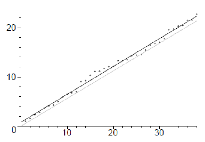
Figure 1. $\log_{2}\log_{2}n$th Mersenne prime verses $n$

http://www.utm.edu/research/primes/mersenne/heuristic.html

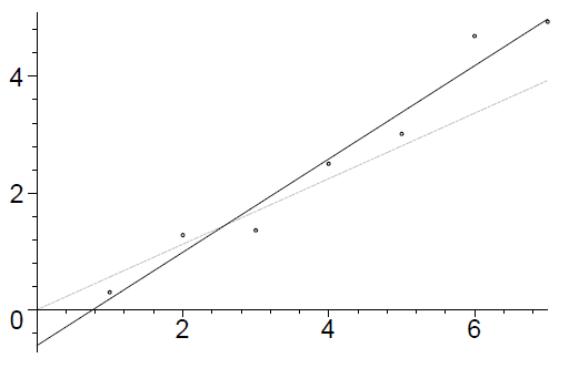
Figure 2. $\log_{10}\log_{10}n$th repunit prime verses $n$

4.2. Cullen and Woodall primes

The Cullen and Woodall primes are $C(n)=n2^{n}+1$, and $W(n)=n2^{n}-1$. In this case we have

$$C(n+p(p-1))\equiv C(n)\pmod{p(p-1)}$$

and

$$W(n+p(p-1))\equiv W(n)\pmod{p(p-1)}\text{.}$$

By the Chinese remainder theorem, both of these have $ord_{p}(2)$ solutions in

$$\{0,1,2,...,p\cdot ord_{p}(2)\},$$

so we might again assume that the probabilities that $p$ divides $C(n)$ and $W(n)$ are both $1/p$ for odd primes $p$–the same as for an arbitrary random integers. But are these probabilities independent for different primes $p$ and $q$? We must ask this because $p(p-1)$ and $q(q-1)$ are not relatively prime. We verify this independence as follows:

Theorem 4.2.

Let $p$ and $q$ be distinct odd primes and let $a$ and $b$ be any integers. The the system of congruences

$$\left\{\begin{array}[]{c}n2^{n}\equiv a\pmod{p}\\ n2^{n}\equiv b\pmod{q}\end{array}\right.$$

has $lcm(pq,ord_{p}(2),ord_{q}(2))/pq$ solutions in $\{0,1,2,...,lcm(pq,ord_{p}(2),ord_{q}(2))\}$.

Proof.

For each $r$ modulo $d=lcm(ord_{p}(2),ord_{q}(2))$ write $n=r+sd$. Then the system above is

$$\left\{\begin{array}[]{c}sd\equiv a/2^{r}-r\pmod{p}\\ sd\equiv b/2^{r}-r\pmod{q}\end{array}\right.$$

Assume that $q$ is the larger of the two primes, then we know $q\nmid ord_{p}(2)$, so the second of these congruences has a unique solution (modulo $q$). If $p\nmid d$, then the first congruence also has a unique solution, giving a total of $d$ solution to the original system (one for each $r$). In this case $d$ is $lcm(pq,ord_{p}(2),ord_{q}(2))/pq$. On the other hand, if $p\mid d$, then the only acceptable choices of $r$ are those for which $r2^{r}\equiv a\pmod{p}$. There are $d/p$ of these–which again is $lcm(pq,ord_{p}(2),ord_{q}(2))/pq$. ∎

For each odd prime the analog of the adjustment factor (2.2) is therefore one, and the complete adjustment factor (2.3) is $2$ in both cases (Cullen and Woodall). This gives us the following.

Conjecture 4.3.

The expected number of Cullen and Woodall primes with $n\leq N$ are each

(4.1) $$2\int_{2}^{N}\frac{dx}{\log x2^{x}}\backsim 2\frac{\log N-\log 2}{\log 2}$$

Table 9 shows us that what little evidence we have does not support (4.1) well for the Cullen numbers, though it does appear reasonable for Woodall numbers.

Table 9. Cullen $C(n)$ and Woodall $W(n)$ primes

	actual (with $n<N)$		predicted
$N$	Woodall	Cullen	integral	ratio
1000	15	2	15	18
10,000	18	5	22	25
100,000	24	10	29	31
500,000	$\geq$26	$\geq$13	33	36
1,000,000			35	38

Since we have so few data points it might offer some insight to graph the expected number of Cullen and Woodall primes below each of the known primes of these forms (see graph ?removed?). If our estimate holds, then this graph would remain “near” the diagonal.

4.3. Primorial primes

Primes of the form $p\#\pm 1$ are sometimes called the primorial primes (a term introduced by H. Dubner as a play on the words prime and factorial). Since $\log p\#$ is the Chebyshev theta function, it is well known that asymptotically $\theta(p)=\log p\#$ is approximately $p$. In fact Dusart [15] has shown

$$\lvert\theta(x)-x\rvert\leq 0.006788\frac{x}{\log x}\text{ \ \ \ \ \ \ for }x\geq 2.89\times 10^{7}.$$

We begin (as usual) noting that by the prime number theorem the probability of a “random” number the size of $p\#\pm 1$ being prime is asymptotically $\frac{1}{p}$. However, $p\#\pm 1$ does not behave like a random variable because primes $q$ less than $p$ divide $1/q^{\text{th}}$ of a random set of integers, but can not divide $p\#\pm 1$. So we adjust our estimate by dividing by $1-\frac{1}{q}$ for each of these primes $q$. By Mertens’ theorem 4.1 our final estimate of the probability that $p\#\pm 1$ is prime is $\frac{e^{\gamma}\log p}{p}$.

By this simple model, the expected number of primes $p\#\pm 1$ with $p\leq N$ would then be

$$\sum_{p\leq N}\frac{e^{\gamma}\log p}{p}\sim e^{\gamma}\log N$$

Conjecture 4.4.

The expected number of primorial primes of each of the forms $p\#\pm 1$ with $p\leq N$ are both approximately $e^{\gamma}\log N$.

The known, albeit limited, data supports this conjecture. What is known is summarized in Table 10.

Table 10. The number of primorial primes $p\#\ \pm 1$ with $p\leq N$

	actual		predicted
$N$	$p\#+1$	$p\#-1$	(of each form)
10	4	2	4
100	6	6	8
1000	7	9	12
10000	13	16	16
100000	19	18	20

Remark 4.5.

By the above estimate, the $n^{\text{th}}$ primorial prime should be about $e^{n/e^{\gamma}}$.

4.4. Factorial primes

The primes of the forms $n!\pm 1$ are regularly called the factorial primes, and like the “primorial primes” $p\#\pm 1$, they may owe their appeal to Euclid’s proof and their simple form. Even though they have now been tested up to $n=10000$ (approximately 36000 digits), there are only $39$ such primes known. To develop a heuristical estimate we begin with Stirling’s formula:

$$\log n!=(n+\frac{1}{2})\log n-n+\frac{1}{2}\log 2\pi+O\left(\frac{1}{n}\right)$$

or more simply: $\log n!\sim n(\log n-1)$. So by the prime number theorem the probability a random number the size of $n!\pm 1$ is prime is asymptotically $\frac{1}{n(\log n-1)}$.

Once again our form, $n!\pm 1$ does not behave like a random variable–this time for several reasons. First, primes $q$ less than $n$ divide $1/q$–th of a set of random integers, but can not divide $n!\pm 1$. So we again divide our estimate by $1-\frac{1}{q}$ for each of these primes $q$ and by Mertens’ theorem we estimate the probability that $n!\pm 1$ is prime to be

(4.2) $$\frac{e^{\gamma}\log n}{n(\log n-1)}.$$

To estimate the number of such primes with $n$ less than $N$, we may integrate this last estimate to get:

Conjecture 4.6.

The expected number of factorial primes of each of the forms $n!\pm 1$ with $n\leq N$ are both asymptotic to $e^{\gamma}\log N$

Table 11 shows a comparison of this estimate to the known results.

Table 11. The number of factorial primes $n!\pm 1$ with $n\leq N$

	actual		predicted
$N$	$n!+1$	$n!-1$	(of each form)
10	3	4	4
100	9	11	8
1000	16	17	12
10000	18	21	16

As an alternate check on this heuristic model, notice that it also applies to the forms $k\cdot n!\pm 1$ ($k$ small). For $1\leq k\leq 500$ and $1\leq n\leq 100$ the form $k\cdot n!+1$ is a prime 4275 times, and the form $k\cdot n!-1$, 4122 times. This yields an average of 8.55 and 8.24 primes for each $k$, relatively close to the predicted $8.20$.

But what of the other obstacles to $n!\pm 1$ behaving randomly? Most importantly, what effect does accounting for Wilson’s theorem have? These turn out not to significantly alter our estimate above. To see this we first we summarize these divisibility properties as follows.

Theorem 4.7.

Let $n$ be a positive integer.

1. $n$ divides $1!-1$ and $0!-1$.

2. If $n$ is prime, then $n$ divides both $(n-1)!+1$ and $(n-2)!-1$.

3. If $n$ is odd and $2n+1$ is prime, then $2n+1$ divides exactly one of $n!\pm 1$.

4. If the prime $p$ divides $n!\pm 1$, then $p-n-1$ divides one of $n!\pm 1$.

Proof.

(ii) is Wilson’s theorem. For (iii), note that if $2n+1$ is prime, then Wilson’s theorem implies

$$-1\equiv 1\cdot 2\cdot\ldots\cdot n\cdot(-n)\cdot\ldots\cdot(-1)\equiv(-1)^{n}(n!)^{2}\pmod{2n+1}.$$

When $n$ is odd this is $(n!)^{2}\equiv 1$, so $n!\equiv\pm 1\pmod{2n+1}$. Finally, to see (iv), suppose $n!\equiv\pm 1\pmod{p}$. Since $(p-1)!\equiv-1$, this is

$$(p-1)(p-2)\cdot\ldots\cdot(n+1)\equiv(-1)^{p-n-1}(p-n-1)!\equiv\mp 1\pmod{p}.$$

This shows $p$ divides exactly one of $(p-n-1)!\pm 1$. ∎

To adjust for the divisibility properties (ii) and (iii), we should multiply our estimate 4.2 by $1-\frac{1}{\log n}$, which is roughly the probability that $n+1$ or $n+2$ is composite; and then by $1-\frac{1}{4\log 2n}$, which is the probability $n$ is odd and $2n+1$ is prime. The other two cases of Theorem 4.7 require no adjustment. This gives us the following estimate of the primality of $n!\pm 1$.

(4.3) $$\left(1-\frac{1}{4\log 2n}\right)\frac{e^{\gamma}}{n}$$

Integrating as above suggests there should be $e^{\gamma}(\log N-\frac{1}{4}\log\log 2N)$ primes of the forms $n!\pm 1$ with $n\leq N$. Since we are using an integral of probabilities in our argument, we can not hope to do much better than an error of $o(\log N)$, so this new estimate is essentially the same as our conjecture above.

References

- [1] E. Bach, The complexity of number-theoretic constants, Inform. Process. Lett. 62 (1997), no. 3, 145–152. MR 98g:11148
- [2] E. Bach and J. Shallit, Algorithmic number theory, Foundations of Computing, vol. I: Efficient Algorithms, The MIT Press, Cambridge, MA, 1996. MR 97e:11157
- [3] P. T. Bateman and R. A. Horn, A heuristic asymptotic formula concerning the distribution of prime numbers, Math. Comp. 16 (1962), 363–367. MR 26 #6139
- [4] by same author, Primes represented by irreducible polynomials in one variable, Proc. Symp. Pure Math. (Providence, RI), vol. VIII, Amer. Math. Soc., 1965, pp. 119–132. MR 31 #1234
- [5] A. Björn and H. Riesel, Factors of generalized Fermat numbers, Math. Comp. 67 (1998), 441–446. MR 98e:11008
- [6] J. M. Borwein, D. M. Bradley, and R. E. Crandall, Computational strategies for the Riemann zeta function, J. Comput. Appl. Math. 121 (2000), no. 1–2, 247–296, Numerical analysis in the 20th century, Vol. I, Approximation. MR 2001h:11110
- [7] R. P. Brent, The distribution of small gaps between succesive primes, Math. Comp. 28 (1974), 315–324. MR 48 #8356
- [8] V. Brun, La serie 1/5 + 1/7 + [etc.] où les denominateurs sont “nombres premiers jumeaux” est convergente ou finie, Bull. Sci. Math. 43 (1919), 100–104,124–128.
- [9] C. Caldwell and Y. Gallot, On the primality of and , Math. Comp. 71 (2002), no. 237, 441–448. MR 2002g:11011
- [10] Lord Cherwell, Note on the distribution of the intervals between primes numbers, Quart. J. Math. Oxford 17 (1946), no. 65, 46–62. MR 8,136e
- [11] Lord Cherwell and E. M. Wright, The frequency of prime-patterns, Quart. J. Math. Oxford 11 (1960), 60–63. MR 24 #A98
- [12] R. Crandall, K. Dilcher, and C. Pomerance, A search for Wieferich and Wilson primes, Math. Comp. 66 (1997), no. 217, 433–449. MR 97c:11004
- [13] L. E. Dickson, A new extention of Dirichlet’s theorem on prime numbers, Messenger Math. 33 (1904), 155–161.
- [14] H. Dubner and Y. Gallot, Distribution of generalized Fermat prime numbers, Math. Comp. 71 (2002), 825–832. MR 2002j:11156
- [15] P. Dusart, The prime is greater than for , Math. Comp. 68 (1999), no. 225, 411–415. MR 99d:11133
- [16] T. Forbes, Prime –tuplets – , M500 146 (1995), 6–8.
- [17] E. Grosswald, Arithmetic progressions that consist only of primes, J. Number Theory 14 (1982), 9–31. MR 83k:10081
- [18] E. Grosswald and Jr. P. Hagis, Arithmetic progression consisting only of primes, Math. Comp. 33 (1979), no. 148, 1343–1352. MR 80k:10054
- [19] H. Halberstam and H.-E. Richert, Sieve methods, Academic Press, 1974. MR 54 #12689
- [20] G. H. Hardy and J. E. Littlewood, Some problems of Diophantine approximation, Acta Math. 37 (1914), 155–238.
- [21] by same author, Some problems of ‘partitio numerorum’ : III: On the expression of a number as a sum of primes, Acta Math. 44 (1923), 1–70, Reprinted in “Collected Papers of G. H. Hardy,” Vol. I, pp. 561-630, Clarendon Press, Oxford, 1966.
- [22] G. H. Hardy and E. M. Wright, An introduction to the theory of numbers, Oxford University Press, 1979. MR 81i:10002
- [23] R. Harley, Some estimates due to Richard Brent applied to the “high jumpers” problem, available on-line: http://pauillac.inria.fr/ harley/wnt.ps, December 1994.
- [24] D. Hensley and I. Richards, On the incompatibility of two conjectures concerning primes, Analytic Number Theory, Proc. Sympos. Pure Math., Vol. XXIV, St. Louis Univ., 1972, Amer. Math. Soc., 1973, pp. 123–127. MR 49 #4950
- [25] by same author, Primes in intervals, Acta. Arith. 25 (1973/74), 375–391. MR 53 #305
- [26] H. Iwanies, Almost-primes represented by quadratic polynomials, Ivent. Math. 47 (1978), 171–188. MR 58 #5553
- [27] D. E. Knuth, The art of computer programming. Volume 1: Fundamental algorithms, Addison-Wesley, Reading, Mass., 1975, 2nd edition, 2nd printing. MR 51 #14624
- [28] G. Löh, Long chains of nearly doubled primes, Math. Comp. 53 (1989), 751–759. MR 90e:11015
- [29] B. H. Mayoh, The second Goldbach conjecture revisited, BIT 8 (1968), 128–133. MR 39 #125
- [30] P. Moree, Approximation of singular series and automata, Manuscripta Math. 101 (2000), 385–399. MR 2001f:11204
- [31] T. Nicely, Enumeration to of the twin primes and Brun’s constant, Virginia Journal of Science 46 (1995), no. 3, 195–204. MR 97e:11014
- [32] G. Pólya, Heuristic reasoning in the theory of numbers, Amer. Math. Monthly 66 (1959), 375–384.
- [33] P. Pritchard, A. Moran, and A. Thyssen, Twenty-two primes in arithmetic progression, Math. Comp. 64 (1995), no. 211, 1337–1339. MR 95j:11003
- [34] P. Ribenboim, The new book of prime number records, 3rd ed., Springer-Verlag, New York, NY, 1995. MR 96k:11112
- [35] I. Richards, On the incompatability of two conjectures concerning primes; a discussion of the use of computers in attacking a theoretical problem, Bull. Amer. Math. Soc. 80 (1973/74), 419–438.
- [36] H. Riesel, Prime numbers and computer methods for factorization, Progress in Mathematics, vol. 126, Birkhäuser Boston, Boston, MA, 1994. MR 95h:11142
- [37] A. Schinzel, Remarks on the paper ‘sur certaines hypothèses concernant les nombres premiers’, Acta. Arith. 7 (1961), 1–8. MR 24 #A70
- [38] M. Schroeder, Number theory in science and communication : With applications in cryptography, physics, digital information, computing, and self-similarity, 3rd ed., Springer-Verlag, New York, NY, 1997. MR 99c:11165
- [39] M. R. Schroeder, Where is the next Mersenne prime hiding?, Math. Intelligencer 5 (1983), no. 3, 31–33. MR 85c:11010
- [40] D. Shanks, On the conjecture of hardy & littlewood concerning the number of primes of the form , Math. Comp. 14 (1962), 321–332. MR 22 #10960
- [41] by same author, Solved and unsolved problems in number theory, Chelsea, New York, NY, 1978. MR 80e:10003
- [42] D. Shanks and S. Kravitz, On the distribution of Mersenne divisors, Math. Comp. 21 (1967), 97–101. MR 36 #3717
- [43] P. Stäckel, Die Darstellung der geraden Zahlen als Summen von zwei Primzahlen, Sitz. Heidelberger Akad. Wiss 7A (1916), no. 10, 1–47.
- [44] S. Wagstaff, Divisors of Mersenne numbers, Math. Comp. 40 (1983), no. 161, 385–397. MR 84j:10052
- [45] J. W. Wrench, Evaluation of Artin’s constant and the twin-prime constant, Math. Comp. 15 (1961), 396–398. MR 23 #A1619
- [46] S. Yates, Sophie Germain primes, The Mathematical Heritage of C. F. Gauss (G. M. Rassias, ed.), World Scientific, 1991, pp. 882–886. MR 93a:11007