A new property of congruence lattices
of slim, planar, semimodular lattices

Abstract.

The systematic study of planar semimodular lattices started in 2007 with a series of papers by G. Grätzer and E. Knapp. These lattices have connections with group theory and geometry. A planar semimodular lattice $L$ is slim if $\mathsf{M}_{3}$ it is not a sublattice of $L$. In his 2016 monograph, “The Congruences of a Finite Lattice, A   Proof-by-Picture Approach”, the second author asked for a characterization of congruence lattices of slim, planar, semimodular lattices. In addition to distributivity, both authors have previously found specific properties of these congruence lattices. In this paper, we present a new property, the Three-pendant Three-crown Property. The proof is based on the first author’s papers: 2014 (multifork extensions), 2017 ($\mathcal{C}_{1}$-diagrams), and a recent paper (lamps), introducing the tools we need.

1. Introduction

1.1. The Main Theorem

The book G. Grätzer [19] presents many results characterizing congruence lattices of various classes of finite lattices, spanning 80 years, up to 2015. In particular, in 1996, G. Grätzer, H. Lakser, and E. T. Schmidt [28] started looking at the class of semimodular lattices and were surprised: every finite distributive lattice can be represented as the congruence lattice of a planar semimodular lattice.

The sublattice $\mathsf{M}_{3}$ played a crucial role in the Grätzer-Lakser-Schmidt construction, so it was natural to ask (see Problems 1 in G. Grätzer [20], originally raised in G. Grätzer [19]) what happens if, in addition to planarity and semimodularity, we also assume that the lattice is slim, that is, it does not have $\mathsf{M}_{3}$ sublattices.

Problem 1.1.

What are the congruence lattices of slim, planar, semimodular lattices?

We call a slim, planar, semimodular lattice an SPS lattice. A finite distributive lattice $D$ is representable by an SPS lattice $L$ (in short, representable) if $D$ is isomorphic to the congruence lattice $\operatorname{Con}L$ of an SPS lattice $L$.

We say that a finite distributive lattice $D$ satisfies the Three-pendant Three-crown Property if the ordered set $R_{3}$ of Figure 1 has no cover-preserving embedding into $\textup{J}(D)$.

Our paper continues the research in G. Czédli [7] that presented four new properties of $\operatorname{Con}L$. We provide one more.

Now we can state our result.

Main Theorem.

Let $L$ be a slim, planar, semimodular lattice. Then $\operatorname{Con}L$ satisfies the Three-pendant Three-crown Property.

We have one more theorem in this paper.

Theorem 1.2.

Let $n$ be a positive integer number and $L_{1}$, …, $L_{n}$ be slim, planar, semimodular lattices with at least three elements. Then there exists a slim rectangular lattice $H$ and a slim patch lattice $L$ such that the following two isomorphisms hold:

$$\operatorname{Con}H \cong\operatorname{Con}{L_{1}}\times\dots\times\operatorname{Con}{L_{n}},$$ (1.1)

$$\operatorname{Con}L \cong\bigl{(}\operatorname{Con}{L_{1}}\times\dots\times\operatorname{Con}{L_{n}}\bigr{)}+\mathsf{B}_{2},$$ (1.2)

In (1.2), the operation $+$ stands for ordinal sum $($the second summand is put on the top of the first one$)$. We define rectangular lattices and patch lattices in Section  2.

1.2. Background

G. Grätzer and E. Knapp [22]–[26] started the study of planar semimodular lattices. There are a number of surveys of this field, see the book chapter G. Czédli and G. Grätzer [9] in G. Grätzer and F. Wehrung, eds.  [32], and G. Czédli and Á. Kurusa [11]. For the topic: congruences of planar semimodular lattices, see the book chapter G. Grätzer [16] in G. Grätzer and F. Wehrung, eds.  [32].

This research have also led to results outside of lattice theory: to a group theoretical result by G. Czédli and E. T. Schmidt [13] and G. Grätzer and J. B. Nation [29], and to (combinatorial) geometric results by G. Czédli [4] and [6], K. Adaricheva and G. Czédli  [1], and G. Czédli and Á. Kurusa [11]. G. Czédli and G. Makay [12] presented a computer game based on these lattices. G. Czédli [8] is a related model theoretic paper.

The next two theorems summarize what we know about congruence lattices of SPS lattices. (In both theorems, the covering relations are those of the ordered set $\textup{J}(\operatorname{Con}L)$ and not of the lattice $\operatorname{Con}L$.)

Theorem 1.3 (G. Grätzer  [20] and [21]).

Let $L$ be an SPS lattice with at least three elements.

1. The ordered set $\textup{J}(\operatorname{Con}L)$ has at least two maximal elements. (Equivalently, $\operatorname{Con}L$ has at least two coatoms.)

2. Every element of the ordered set $\textup{J}(\operatorname{Con}L)$ has at most two covers.

The three element chain is an example that the necessary condition (i) for representability is not sufficient. G. Czédli [3] gave an eight element distributive lattice to show that the necessary condition (ii) for representability is not sufficient. See also G. Grätzer [18].

Our paper is a continuation of G. Czédli [7]. Here are some of the results of this paper.

Theorem 1.4 (G. Czédli [7]).

Let $L$ be an SPS lattice with at least three elements.

1. The set of maximal elements of the ordered set $\textup{J}(\operatorname{Con}L)$ can be represented as the disjoint union of two nonempty subsets such that no two distinct elements in the same subset have a common lower cover.

2. The ordered set $R$ of  Figure 1 cannot be embedded as a cover-preserving subset into the ordered set $\textup{J}(\operatorname{Con}L)$ provided that any maximal element of $R$ is a maximal element of $\textup{J}(\operatorname{Con}L)$.

3. If $x\in\textup{J}(\operatorname{Con}L))$ is covered by a maximal element $y$ of $\textup{J}(\operatorname{Con}L)$, then $y$ is not the only cover of $x$ in the ordered set $\textup{J}(\operatorname{Con}L)$.

4. Let $x\neq y\in\textup{J}(\operatorname{Con}L)$, and let $z$ be a maximal element of $\textup{J}(\operatorname{Con}L)$. Assume that both $x$ and $y$ are covered by $z$ in the ordered set $\textup{J}(\operatorname{Con}L)$. Then there is no element $u\in\textup{J}(\operatorname{Con}L)$ such that $u$ is covered by $x$ and $y$ in $\textup{J}(\operatorname{Con}L)$.

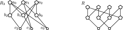
Figure 1. The Three-pendant Three-crown ordered set $R_{3}$ and the Two-pendant Four-crown ordered set $R$; the elements of the crowns are pentagons

Outline

Section 2 recalls some concepts. Section 3 recalls some of the tools developed in G. Czédli [7] while we develop some new tools in Section 4. We prove our Main Theorem in Section 5. Finally, Section 6 proves Theorem 1.2 and discusses what we know about the congruence lattices of slim patch lattices.

2. Basic notation and concepts

All lattices in this paper are finite. We assume that the reader is familiar is with the rudiments of lattice theory. Most basic concepts and notation not defined in this paper are available in Part I of the monograph G. Grätzer [19], which is free to access. In particular, the glued sum of two lattices $A$ and $B$ is denoted by $A\overset{\textbf{.}}{+}B$ ($B$ is on the top of $A$ with the unit element of $A$ and the zero of $B$ identified, so $\mathsf{C}_{2}\overset{\textbf{.}}{+}\mathsf{C}_{2}$ is $\mathsf{C}_{3}$). The $n$-element chain is $\mathsf{C}_{n}$, the Boolean lattice with $n$ atoms is $\mathsf{B}_{n}$, and $\mathsf{M}_{3}$ is the $5$-element modular nondistributive lattice. The set of maximal elements of an ordered set $P$ will be denoted by $\textup{Max}(P)$. In this paper, edges are synonymous with prime intervals.

For a finite lattice $L$, the set of (non-zero) join-irreducible elements and (non-unit) meet-irreducible elements will be denoted by $\textup{J}(L)$ and $\textup{M}(L)$, respectively, so $\textup{J}(L)\cap\textup{M}(L)$ is the set of doubly irreducible elements. We denote by $x^{*}$ the unique cover of $x$ for $x\in\textup{M}(L)$. For an element $a\in L$, let $\mathord{\downarrow}\,a=\{\,x\in L\mid x\leq a\,\}$ be the principal ideal generated by $a$ and $\mathord{\uparrow}\,a=\{\,x\in L\mid x\geq a\,\}$ the principal filter generated by $a$.

A planar semimodular lattice is slim if it does not contain $\mathsf{M}_{3}$ as a sublattice; see G. Grätzer and E. Knapp [22], [25], G. Czédli and E. T. Schmidt [13].

Let $L$ be a planar lattice. A left corner $\textup{lc}(L)$ (resp., right corner $\textup{rc}(L)$) of $L$ is a doubly-irreducible element in $L-\{0,1\}$ on the left (resp., right) boundary of $L$. We define a rectangular lattice $L$ as a planar semimodular lattice which has exactly one left corner, $\textup{lc}(L)$, and exactly one right corner, $\textup{rc}(L)$, and they are complementary, that is, $\textup{lc}(L)\vee\textup{rc}(L)=1$ and $\textup{lc}(L)\wedge\textup{rc}(L)=1$ (see G. Grätzer and E. Knapp [22]). Finally, a rectangular lattice in which both corners are coatoms are called a patch lattice.

3. Tools

In this section, $L$ is a slim rectangular lattice with a fixed $\mathcal{C}_{1}$-diagram, as we shall soon define.

We call the directions of $(1,1)$ and $(1,-1)$ normal and any direction $(\cos\alpha,\sin\alpha)$ with $\pi/2<\alpha<3\pi/2$ steep. (In [5] and other papers, the first author uses “precipitous” instead of “steep”.) Edges and lines parallel to a steep vector are also called steep, and similarly for normal slopes.

The following definition and result are crucial in the study of SPS lattices.

Definition 3.1 (G. Czédli [5]).

A diagram of the slim rectangular lattice $L$ is a $\mathcal{C}_{1}$-diagram if it has the following two properties.

1. If $x\in\textup{M}(L)-(\mathord{\uparrow}\,\textup{lc}(L)\cup\mathord{\uparrow}\,\textup{rc}(L))$, then the edge $[x,x^{*}]$ is steep.

2. Every edge not of the form $[x,x^{*}]$ as in (i) has a normal slope.

If, in addition,

1. any two edges on the lower boundary are of the same geometric length,

then the diagram is a $\mathcal{C}_{2}$-diagram.

Theorem 3.2 (G. Czédli [5]).

Every slim rectangular lattice $L$ has a $\mathcal{C}_{2}$-diagram.

The chains $\mathord{\downarrow}\,\textup{lc}(L)$, $\mathord{\uparrow}\,\textup{lc}(L)$, $\mathord{\downarrow}\,\textup{rc}(L)$, and $\mathord{\uparrow}\,\textup{rc}(L)$ are called the bottom left boundary chain, …, top right boundary chain. These chains have normal slopes and they are the sides of a geometric rectangle, which we call the full geometric rectangle of $L$ and denote it by $\textup{FulR}(L)$. The four vertices of this rectangle are $0$, $1$, $\textup{lc}(L)$, and $\textup{rc}(L)$. The lower boundary of $L$ is $\mathord{\downarrow}\,\textup{lc}(L)\cup\mathord{\downarrow}\,\textup{rc}(L)$ and the upper boundary is $\mathord{\uparrow}\,\textup{lc}(L)\cup\mathord{\uparrow}\,\textup{rc}(L)$. With the exception of the corners, no meet-irreducible element belongs to the lower boundary of $L$.

The following is the central definition of G. Czédli [7].

Definition 3.3.

(A) Let $L$ be a slim rectangular lattice. The edges $[x,y]$ of $L$ with $x\in\textup{M}(L)$ are called neon tubes. We call a neon tube $[x,y]$ on the upper boundary of $L$, a boundary neon tube; it is an internal neon tube, otherwise. Equivalently, neon tubes with normal slopes are boundary neon tubes, while steep neon tubes are internal.

In Figures 2, 9, and 10, we represent the neon tubes by thick edges.

(B) A boundary neon tube ${\mathfrak{n}}=[p,q]$ is also called a boundary lamp. This lamp $I$ is an edge, the neon tube ${\mathfrak{n}}$ is the neon tube of the lamp $I$. Define $\textup{Foot}(I)$ as $p$ and $\textup{Peak}(I)$ as $q$. If $\textup{Foot}(I)$ is on the top left boundary chain, then $I$ is a left boundary lamp; similarly, we define right boundary lamps.

In Figure 2, the left boundary lamps and the right boundary lamps are $P_{1},\dots,P_{5}$ and $Q_{1},\dots,Q_{6}$, respectively, and $p_{i}=\textup{Foot}(P_{i})$ and $q_{j}=\textup{Foot}(Q_{j})$ for all $i$ and $j$.

(C) Every steep (that is, internal) neon tube ${\mathfrak{n}}=[p,q]$ belongs to a unique internal lamp $I=[\beta_{q},q]$, where $\beta_{q}$ is the meet of all $p^{\prime}\in L$ such that $[p^{\prime},q]$ is a steep neon tube. For the lamp $I$, define the $\textup{Foot}(I)$ as $\beta_{q}$ and the peak $\textup{Peak}(I)$ as $q$.

In Figure 2, there are five internal lamps, $A,\dots,E$ with $\textup{Foot}(A)=a$, $\textup{Foot}(B)=b$, and so on; also, $\textup{Peak}(A)=g$, $\textup{Peak}(B)=h$, and $\textup{Peak}(C)=z$; so $A=[a,g]$, $B=[b,h]$, and $C=[c,z]$.

(D) The set $\textup{Lamp}(L)$ consists of all lamps of $L$. For example, for the lattice $L$ in Figure 2, there are $16$ lamps in $L$.

(E) A lamp $I$ determines a geometric region (as in David Kelly and I. Rival [30]) which we call the body of $I$, and denote it by $\textup{Body}(I)$. It has a geometric shape: it is either a line segment or a quadrilateral whose lower sides have normal slopes and whose upper sides are steep.

In Figure 2, the regions $\textup{Body}(A)$, $\textup{Body}(B)$, and $\textup{Body}(C)$ are colored dark-grey.

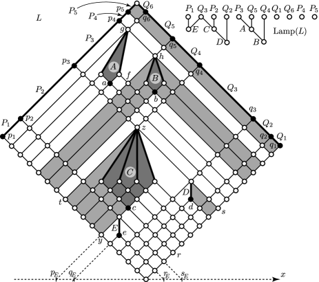
Figure 2. Lamps and related geometric objects

For later reference, we recall by G. Czédli [7, Lemma 3.1] that

A lamp is uniquely determined by its foot. (3.1)

The feet of our lamps are black-filled in Figures 2–10; this helps us find them.

In the real world, lamps emit light. Our lamps do it in a special way: the light rays go from all points of the neon tubes of a lamp $I$ downward with normal slopes. Next we give our definition of light emission. For an element $x\in L$, we define the line segment $\textup{Line}_{\textup{L}}(x)$ from $x$ left and down, of normal slope to the lower-right boundary of $L$. Similarly, to the right, we have $\textup{Line}_{\textup{R}}(x)$.

So for a lamp $I$, we have the four line segments, from $\textup{Peak}(I)$ and $\textup{Foot}(I)$, left and right. We denote them by $\textup{LRoof}(I)$ (the left roof), $\textup{RRoof}(I)$ (the right roof), $\textup{LFloor}(I)$, (the left floor) and $\textup{RFloor}(I)$ (the right floor).

Definition 3.4 (G. Czédli [7]).

For a lamp $I$ of a slim rectangular lattice $L$, we define

1. the area left lit by $I$ (or, as in [7], illuminated from the right by $I$), denoted by $\textup{LeftLit}(I)$, is a quadrangle bounded by the line segments $\textup{Line}_{\textup{L}}(\textup{Peak}(I))$, $\textup{Line}_{\textup{L}}(\textup{Foot}(I))$, the upper right boundary of $I$, and the appropriate line segment of the lower left boundary of $L$.

2. the area right lit by $I$, denoted by $\textup{RightLit}(I)$, is defined symmetrically.

3. the area lit by $I$, denoted by $\textup{Lit}(I)$ is defined as $\textup{LeftLit}(I)\cup\textup{RightLit}(I)$. The geometric (topological) interior of $\textup{Lit}(L)$ is denoted by $\textup{OLit}(L)$ and we call it the open lit set of $I$.

For example, in Figure 2, $\textup{LeftLit}(C)$, $\textup{RightLit}(D)$, and $\textup{Lit}(B)$ are shaded.

It follows from the statements (2.10) and (2.11) of G. Czédli [7] that, for every lamp $I$ of $L$,

the geometric (that is, topological) boundaries of the areas $$\textup{Lit}(I) \textup{LeftLit}(I) \textup{RightLit}(I)$$, , and consist of edges. (3.2)

Utilizing the concept of lit sets, we define some relations on $\textup{Lamp}(L)$; G. Czédli [7, Definition 2.9] defines eight relations but here we only need four.

Definition 3.5 (G. Czédli [7]).

Let $L$ be a slim rectangular lattice. We define four relations ${{\rho}}_{\textup{Body}}$, ${{\rho}}_{\textup{foot}}$, ${{\rho}}_{\textup{infoot}}$, and ${{\rho}}_{\textup{alg}}$ on the set $\textup{Lamp}(L)$, by the following rules. For $I,J\in\textup{Lamp}(L)$,

1. $(I,J)\in{{\rho}}_{\textup{Body}}$ if $I\neq J$, $\textup{Body}(I)\subseteq\textup{Lit}(J)$, and $I$ is an internal lamp;

2. $(I,J)\in{{\rho}}_{\textup{foot}}$ if $I\neq J$, $\textup{Foot}(I)\in\textup{Lit}(J)$, and $I$ is an internal lamp;

3. $(I,J)\in{{\rho}}_{\textup{infoot}}$ if $I\neq J$, $\textup{Foot}(I)\in\textup{OLit}(J)$, and $I$ is an internal lamp;

4. $(I,J)\in{{\rho}}_{\textup{alg}}$ if $\textup{Peak}(I)\leq\textup{Peak}(J)$, $\textup{Foot}(I)\not\nleq\textup{Foot}(J)$, and $I$ is an internal lamp.

The significance of lamps becomes clear from the following statement, which is a part of the (Main) Lemma 2.11 of G. Czédli [7].

Lemma 3.6 (G. Czédli [7]).

Let $L$ be a slim rectangular lattice. Then ${{\rho}}_{\textup{Body}}={{\rho}}_{\textup{foot}}={{\rho}}_{\textup{infoot}}={{\rho}}_{\textup{alg}}$. Let ${{\rho}}$ stand for any one (or all) of these relations and let $\leq$ be the reflexive transitive closure of ${{\rho}}$. Then $(\textup{Lamp}(L),\leq)$ is an ordered set and it is isomorphic to $\textup{J}(\operatorname{Con}L)$. Also, if $I,J\in\textup{Lamp}(L)$ and $I\prec J$ in $(\textup{Lamp}(L),\leq)$, then $(I,J)\in{{\rho}}$.

This lemma is illustrated by Figure 2. The isomorphism

$$\textup{Lamp}(L)\cong\textup{J}(\operatorname{Con}L)$$

is witnessed by the map

$$\textup{Lamp}(L)\to\textup{J}(\operatorname{Con}L),\text{ defined by }I\mapsto\textup{con}(\textup{Foot}(I),\textup{Peak}(I)).$$

We also need the following statement.

Lemma 3.7 (G. Grätzer and E. Knapp [25]).

If $K$ is a slim planar semimodular lattice with at least three elements, then there exists a slim rectangular lattice $L$ such that $\operatorname{Con}K\cong\operatorname{Con}L$.

G. Grätzer and E. Knapp [25] proved a stronger statement, which we do not require. See also G. Grätzer and E. T. Schmidt [31].

To verify the Three-pendant Three-crown Property, we have to work in $\textup{J}(\operatorname{Con}L)$. So by utilizing Lemmas 3.6 and 3.7, we can confine ourselves to investigate lamps in slim rectangular lattices.

4. Further tools and the Key Lemma

4.1. Coordinate quadruples

We start with some technical tools.

Definition 4.1.

Let $I$ be a lamp of a slim rectangular lattice $L$ with a fixed $\mathcal{C}_{1}$-diagram. Assume that we choose the coordinate system of the plane $\mathbb{R}^{2}$ so that $(0,0)$ is the zero of $L$.

1. Following G. Czédli [7], the lit set $\textup{Lit}(I)$ of an internal lamp $I$ is bordered by the line segments $\textup{LRoof}(I)$ and $\textup{RRoof}(I)$, $\textup{LFloor}(I)$, and $\textup{RFloor}(I)$, and the appropriate segments on the lower boundary. If $I$ is a boundary lamp, the above-mentioned line segments still border $\textup{Lit}(I)$. Any proper line segment lies on a line referred to as its carrier line.

2. Let $(p_{I},0)$, $(q_{I},0)$, $(r_{I},0)$ and $(s_{I},0)\in\mathbb{R}^{2}$ be the intersection points of the $x$-axis with the carrier lines of $\textup{LRoof}(I)$, $\textup{LFloor}(I)$, $\textup{RFloor}(I)$, and $\textup{RRoof}(I)$, respectively. Then $(p_{I},q_{I},r_{I},s_{I})$ is called the coordinate quadruple of the lamp $I$.

3. Let $I,J\in\textup{Lamp}(L)$. Then $I$ is to the left of $J$, in notation $I\mathrel{\lambda}J$, if $q_{I}\leq p_{J}$ and $s_{I}\leq r_{J}$.

For example, in Figure 2, $\textup{LRoof}(C)$, $\textup{RRoof}(C)$, $\textup{LFloor}(C)$, and $\textup{RFloor}(C)$ are the line segments corresponding to the intervals (in fact, chains) $[t,z]$, $[s,z]$, $[y,c]$, and $[r,c]$, respectively. The coordinate quadruple of the lamp $E$ is shown in Figure 2 and, for example, $E\mathrel{\lambda}D$ and $P_{1}\mathrel{\lambda}C$; however, $P_{2}\mathrel{\lambda}C$ and $A\mathrel{\lambda}B$ fail. For $I\in\textup{Lamp}(L)$, the following observation follow from the definitions.

$$p_{I}<q_{I}<r_{I}<s_{I} I p_{I}=q_{I}<r_{I}<s_{I} I p_{I}<q_{I}<r_{I}=s_{I} I$$ if and only if is an internal lamp, if and only if is a left boundary lamp, if and only if is a right boundary lamp. (4.1)

Remark 4.2.

Apart from an order isomorphism, $(-p_{I},s_{I})$ and $(-q_{I},r_{I})$ are the join-coordinates of $\textup{Peak}(I)$ and $\textup{Foot}(I)$ as in Czédli [5, Definition 4.2].

4.2. Key Lemma

The proof of the Main Theorem is based on the following key result.

Lemma 4.3 (Key Lemma).

Let $I$ and $I^{\prime}$ be lamps of a slim rectangular lattice $L$ with a fixed $\mathcal{C}_{1}$-diagram. If $I\neq I^{\prime}$ and they have a common lower cover in $(\textup{Lamp}(L);\leq)$, then either $I$ is to the left of $I^{\prime}$ or $I^{\prime}$ is to the left of $I$.

Proof.

For later use, recall the following statement G. Czédli [5, Corollary 6.1].

For $$u\neq v\in L u<v y u v u v$$, the inequality holds if and only if the ordinate (that is, the vertical -coordinate) of is less than that of and the geometric line through and is either steep or it has a normal slope. (4.2)

In the rest of this proof, assume that $I\neq I^{\prime}$ are lamps of $L$ and they have a common lower cover $I^{\prime\prime}$ and so incomparable, in notation, $I\parallel I^{\prime}$. By Lemma 3.6, both $(I^{\prime\prime},I)$ and $(I^{\prime\prime},I^{\prime})$ belong to ${{\rho}}_{\textup{infoot}}$, that is, $\textup{Foot}(I^{\prime\prime})\in\textup{OLit}(I)$ and $\textup{Foot}(I^{\prime\prime})\in\textup{OLit}(I^{\prime})$. Hence,

$$\textup{OLit}(I)\cap\textup{OLit}(I^{\prime})\neq\varnothing.$$ (4.3)

As Figure 2 (for the lamp $E$) shows or alternatively, as Remark 4.2 yields,

$$(p_{I},s_{I}) (q_{I},r_{I}) (p_{I},q_{I},r_{I},s_{I}) \textup{Peak}(I) \textup{Foot}(I) I$$, , and determine , , and , respectively; (4.4)

and similarly for $I^{\prime}$. Since $I$ and $I^{\prime}$ are distinct, it follows from (4.3) that

At least one of $$I I^{\prime}$$ and is not a left boundary lamp. Similarly, at least one is not a right boundary lamp. (4.5)

To make the proof more readable, we write $(p,q,r,s)$ for $(p_{I},q_{I},r_{I},s_{I})$ and $(p^{\prime},q^{\prime},r^{\prime},s^{\prime})$ for $(p_{I^{\prime}},q_{I^{\prime}},r_{I^{\prime}},s_{I^{\prime}})$.

Statement (4.5) and G. Czédli [7, Lemma 3.8] yield that

$$q\neq q^{\prime}\quad\text{ and }\quad r\neq r^{\prime}.$$ (4.6)

We distinguish several cases.

Case 1: Both $I$ and $I^{\prime}$ are internal lamps.

We need the following concept (which is based on the concept of circumscribed rectangles by G. Czédli [7, Definition 2.6]) as visualized by Figure 2. For an internal lamp $J\in\textup{Lamp}(L)$, the left shield and the right shield of $J$ are the left upper side and the right upper side of the circumscribed rectangle of $J$. So these shields are line segments. Namely, it follows from (2.8), (2.10), (2.14), and Definition 2.6 of G. Czédli [7] (and from the fact that $\textup{Foot}(J)$ is in the interior of the circumscribed rectangle of $J$) that

the right shield of an internal lamp $$J \textup{LRoof}(J) \textup{LFloor}(J) J$$ is an edge of normal slope and this edge is longer than the geometric distance of (the carrier lines of) and . Analogously for the left shield of . (4.7)

Based on (4.7), there is another way to define the shields of an internal lamp $J$: the left shield of $J$ is the unique edge of slope $(-1,-1)$ whose top is $\textup{Peak}(J)$; the right shield of $J$ has slope $(1,-1)$ and its top is $\textup{Peak}(J)$. For example, in Figure 2, $[h,g]$ is the right shield of $A$ while $[f,h]$ and $[y,\textup{Peak}(E)]$ are the left shields of $B$ and $E$, respectively.

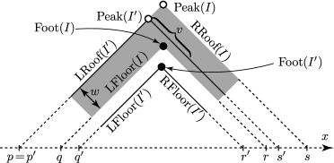
Figure 3. Proving (4.10)

We know from (2.7) of G. Czédli [7] that distinct internal lamps have distinct peaks. This fact along with (3.1) and (4.4) yield that

$$(p,s)\neq(p^{\prime},s^{\prime})\quad\text{ and }\quad(q,r)\neq(q^{\prime},r^{\prime}).$$ (4.8)

Next, we claim that

$$p\neq p^{\prime}.$$ (4.9)

By way of contradiction, assume that $p=p^{\prime}$. Since $q\neq q^{\prime}$ by (4.6) and the role of $I$ and $I^{\prime}$ is now symmetric, we can assume that $q<q^{\prime}$. Since $p=p^{\prime}$ and (4.8) yield that $s\neq s^{\prime}$, we conclude that either $s<s^{\prime}$ or $s^{\prime}<s$.

Case 1A: $s^{\prime}<s$. The situation (apart from the position of  $r^{\prime}$) is illustrated by Figure 3, where $\textup{Lit}(I)$ is the grey area and $\textup{Lit}(I^{\prime})$ is given by its boundary line segments $\textup{LRoof}(I^{\prime})$, $\textup{LFloor}(I^{\prime})$, etc. The figure indicates the length $v$ of the right shield of $I^{\prime}$, which is greater than the “width” $(q^{\prime}-p^{\prime})/\sqrt{2}$ of $\textup{LeftLit}(I^{\prime})$ by (4.7), and the “width” $w=(q-p)/\sqrt{2}=(q-p^{\prime})/\sqrt{2}$ of $\textup{LeftLit}(I)$. By (3.2), the geometric boundary of $\textup{LeftLit}(I)$ consists of edges (but these are not indicated in the figure between $\textup{Foot}(I)$ and $\textup{Peak}(I)$). Since $v>w$, the geometric boundary of $\textup{LeftLit}(I)$ (consisting of edges) crosses the right shield of $I^{\prime}$. But this contradicts the planarity of the diagram since this right shield is an edge by (4.7).

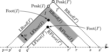
Figure 4. Still proving (4.10)

Case 1B: $s<s^{\prime}$. This case is illustrated by Figure 4 (in which additional conditions hold, such as, $r^{\prime}<r$). In this subcase, $q<q^{\prime}$ yields that $\textup{Foot}(I)$, which is on a line with point $(q,0)$ and of slope $(1,1)$ is above the carrier line of $\textup{LFloor}(I^{\prime})$. Hence, it is clear by the figure and, mainly by (4.2), that $\textup{Peak}(I)\leq\textup{Peak}(I^{\prime})$ but $\textup{Foot}(I)\nleq\textup{Foot}(I^{\prime})$. Thus, $(I,I^{\prime})\in{{\rho}}_{\textup{alg}}$, contradicting that $I\parallel I^{\prime}$. This completes Case 1B and proves (4.9).

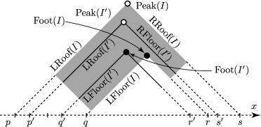
Figure 5. Case $p<p^{\prime}<q$

Next, we are going to show that

if $$p\leq p^{\prime} q\leq p^{\prime}$$, then . (4.10)

So assume that $p\leq p^{\prime}$. Then we know from (4.9) that $p<p^{\prime}$. By way of contradiction, assume that (4.10) fails, that is, $p^{\prime}<q$. Then neither $q^{\prime}=q$, nor $q^{\prime}>q$ by Lemma 3.8 of G. Czédli [7]. So $p<p^{\prime}<q^{\prime}<q$, see Figure 5. Observe that the geometric boundary of $\textup{LeftLit}(I^{\prime})$ cannot cross the right shield of $I$ by (3.2) and (4.7). So we obtain from (4.2) that $\textup{Peak}(I^{\prime})\leq\textup{Peak}(I)$. Note that $\textup{Foot}(I^{\prime})$ is on the carrier line of $\textup{LFloor}(I^{\prime})$, which goes through the point $(q^{\prime},0)$; moreover, $q^{\prime}<q$. Therefore, (4.2) also yields that $\textup{Foot}(I^{\prime})\nleq\textup{Foot}(I)$. Hence, $(I^{\prime},I)\in{{\rho}}_{\textup{alg}}$, contradicting that $I\parallel I^{\prime}$. This contradicts that $p^{\prime}<q$ and so proves the validity of (4.10).

As a variant of (4.10), observe that

if $$s^{\prime}\leq s s^{\prime}\leq r s\leq s^{\prime} s\leq r^{\prime}$$, then . Also, if , then . (4.11)

Indeed, the first part of (4.11) follows from (4.10) by left-right symmetry while its second part follows from the first part by interchanging the role of $I$ and $I^{\prime}$.

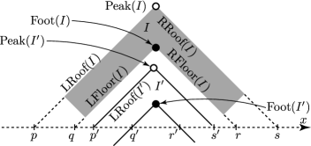
Figure 6. If $p<p^{\prime}$ and $s^{\prime}<s$

Next, we claim that

$$\text{if }\,p\leq p^{\prime},\,\text{ then }\,I\mathrel{\lambda}I^{\prime}.$$ (4.12)

So assume that $p\leq p^{\prime}$. By (4.10), we have that $q\leq p^{\prime}$. We claim that $s\leq s^{\prime}$. Assume to the contrary, that $s^{\prime}<s$. By (4.11), $s^{\prime}\leq r$; see Figure 6. Hence, $\textup{OLit}(I)\cap\textup{OLit}(I^{\prime})=\varnothing$, contradicting (4.3). This shows that $s\leq s^{\prime}$. Applying (4.11), we obtain that $s\leq r^{\prime}$. Now, as part (iii) of Definition 4.1 shows, $q\leq p^{\prime}$ and $s\leq r^{\prime}$ complete the argument proving (4.12).

Since $I$ and $I^{\prime}$ play a symmetric role, we can assume that $p\leq p^{\prime}$. Thus, (4.12) yields the validity of the lemma for the case of internal lamps.

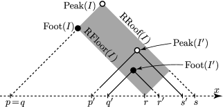
Figure 7. $I$ is a left boundary lamp and $r<r^{\prime}<s$

Case 2: Of the two lamps, $I$ and $I^{\prime}$, one is a boundary lamp and the other one is internal. By symmetry, we can assume that $I$ is a left boundary lamp and $I^{\prime}$ is an internal lamp. By (4.1), $p=q$. Since this is clearly the least possible value, $q\leq p^{\prime}$. Hence, to show that $I\mathrel{\lambda}I^{\prime}$, we need to show that $s\leq r^{\prime}$.

Suppose, for a contradiction, that $r^{\prime}<s$. If $r^{\prime}<r$, then we also have that $s^{\prime}\leq r$; otherwise, $\textup{RFloor}(I)$ would cross the left shield of $I^{\prime}$ (see Figure 6 after collapsing $p$ and $q$). So if $r^{\prime}<r$, then $s^{\prime}\leq r$, but then $\textup{OLit}(I)\cap\textup{OLit}(I^{\prime})=\varnothing$ (similarly to Figure 6 but now $p=q$ and $\textup{LeftLit}(I)$ reduces to a line segment), and this equality contradicts (4.3). This rules out that $r^{\prime}<r$. Since $r^{\prime}=r$ is also ruled out by Lemma 3.8 of G. Czédli [7], we have that $r<r^{\prime}$.

So we have that $r<r^{\prime}<s$; see Figure 7. Combining (4.2) and $r<r^{\prime}$, we obtain that $\textup{Foot}(I^{\prime})\nleq\textup{Foot}(I)$. Thus $\textup{Peak}(I^{\prime})\nleq\textup{Peak}(I)$; indeed, otherwise we would have that $(I^{\prime},I)\in{{\rho}}_{\textup{alg}}$ and so $I^{\prime}\leq I$ would contradict $I\parallel I^{\prime}$. Since $s^{\prime}\leq s$ (together with the trivial $p\leq p^{\prime}$) would imply that $\textup{Peak}(I^{\prime})\leq\textup{Peak}(I)$, which has just been excluded, we obtain that, as opposed to what Figure 7 shows, $s<s^{\prime}$. However, then $r^{\prime}<s<s^{\prime}$ and $\textup{RRoof}(I)$ crosses the left shield of $I^{\prime}$, which contradicts (3.2), (4.7), and the planarity of $L$. We have shown that $I\mathrel{\lambda}I^{\prime}$, as required.

Case 3: Both $I$ and $I^{\prime}$ are boundary lamps. If they both were left boundary lamps, then $\textup{OLit}(I)\cap\textup{OLit}(I^{\prime})$ would contradict (4.3). We would have the same contradiction if both were right boundary lamps. Hence one of them, say $I$, is a left boundary lamp while the other, $I^{\prime}$, is a right boundary lamp, and the required $I\mathrel{\lambda}I^{\prime}$ trivially holds. This completes the proof of Lemma 4.3. ∎

Figure 8. $A_{0}$, $A_{1}$, $A_{2}$, and $B_{1}$

5. Proving the Main Theorem

Now we are ready to prove our main result.

Proof of the Main Theorem.

The theorem is trivial for lattices with less than three elements. Hence, by Lemma 3.7, it suffices to prove the theorem for slim rectangular lattices. By way of contradiction, assume that $L$ is a slim rectangular lattice that fails the 3P3C-property. Then by Lemma 3.6, $R_{3}$ is a cover-preserving ordered subset of $\textup{Lamp}(L)$. Let $X_{i}$ be the lamp corresponding to $x_{i}\in R_{3}$. It follows from Lemma 4.3 that for any $i\neq j\in\{0,1,2\}$, either $A_{i}$ is to the left of $A_{j}$ (in notation, $A_{i}\mathrel{\lambda}A_{j}$), or $A_{j}\mathrel{\lambda}A_{i}$. Therefore, since any permutation of $\{A_{0},A_{1},A_{2}\}$ extends to an automorphism of $R_{3}$, we can assume that $A_{0}\mathrel{\lambda}A_{1}$ and $A_{1}\mathrel{\lambda}A_{2}$; see Figure 8, where the coordinate quadruple of $A_{i}$ is $(p_{i},q_{i},r_{i},s_{i})$. By Definition 4.1(iii), it follows that

$$q_{0}\leq p_{1},\,\,s_{0}\leq r_{1},\,\,q_{1}\leq p_{2},\,\,s_{1}\leq r_{2},\text{ and }p_{i}\leq q_{i}\leq r_{i}\leq s_{i}$$ (5.1)

for every $i\in\{0,1,2\}$. Note that $A_{0}$ is either an internal lamp such as in the figure, or it is a left boundary lamp and then $\textup{LeftLit}(A_{0})$ is only a line segment, and analogously for $A_{2}$. Let $(p^{\prime},q^{\prime},r^{\prime},s^{\prime})$ denote the coordinate tuple of $B_{1}$; note that $\textup{Lit}(B_{1})$ is grey in the figure. It follows from (5.1) and from trivial properties of $\mathcal{C}_{1}$-diagrams that $\textup{OLit}(A_{1})\cap\textup{OLit}(B_{1})=\varnothing$. On the other hand, $C_{1}\prec A_{1}$ and $C_{1}\prec B_{1}$ give that $(C_{1},A_{1})\in{{\rho}}_{\textup{infoot}}$ and $(C_{1},B_{1})\in{{\rho}}_{\textup{infoot}}$ by Lemma 3.6. It follows that $\textup{Foot}(C_{1})\in\textup{OLit}(A_{1})\cap\textup{OLit}(B_{1})=\varnothing$, which is a contradiction, completing the proof of the Main Theorem. ∎

6. Rectangular and patch lattices

Let $(A,\rho)$ and $(A^{\prime},\rho^{\prime})$ be ordered sets. Their cardinal sum will be denoted by $(A,\rho)\mathop{\dot{\cup}}(A^{\prime},\rho^{\prime})$; it is $(A\sqcup A^{\prime},\rho\sqcup\rho^{\prime})$ where $\sqcup$ stands for disjoint union. The operation $\overset{\textbf{.}}{+}$ for glued sum was defined at the beginning of Section 2.

6.1. Proving Theorem 1.2

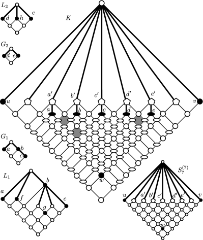
Figure 9. Constructing $K$ from $L_{1}$ and $L_{2}$

By Lemma 3.7, we can assume that $L_{1}$, …, $L_{n}$ are slim rectangular lattices.

First, we deal with (1.1). It follows from G. Birkhoff’s classical Representation Theorem of Finite Distributive Lattices, see, for example, G. Grätzer  [15, Theorem 107], that it suffices to find a slim planar semimodular lattice $H$ such that

$$\textup{J}(H)\cong\textup{J}(L_{1})\mathop{\dot{\cup}}\cdots\mathop{\dot{\cup}}\textup{J}(L_{n});$$ (6.1)

Let $H=L_{1}\overset{\textbf{.}}{+}\cdots\overset{\textbf{.}}{+}L_{n}$. Observe the each edge of $H$ is an edge of a unique summand. For $i\in\{1,,\dots,n\}$, let ${\mathfrak{p}}_{i}$ be an edge of $L_{i}$. This easily implies that, for $i,j\in\{1,\dots,n\}$, $\textup{con}({\mathfrak{p}}_{i})$ does not collapse ${\mathfrak{p}}_{j}$ provided that $i\neq j$. The most convenient way to see this is by applying the Swing Lemma from G. Grätzer  [17]; see also G. Czédli, G. Grätzer, and Lakser [10] and G. Czédli and G. Makay [12]. This implies (6.1) and proves the (1.1)-part of the theorem.

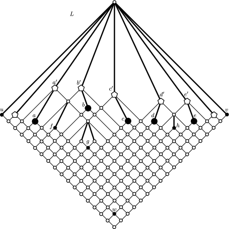
Figure 10. Constructing $L$ from $K$, $L_{1}$, and $L_{2}$

To prove (1.2), we assume some familiarity with the multifork extensions of G. Czédli [2]. Recall that the grid of the slim rectangular lattice $L_{i}$ is its sublattice generated by the upper boundary of $L_{i}$. This grid will be denoted by $G_{i}$; it is a distributive lattice with all if its edges of normal slopes.

For $i\in\{1,\dots,n\}$, let $t_{i}$ be the number of boundary lamps of $L_{i}$, and let $t=t_{1}+\cdots+t_{n}+2$. We start our construction by taking $S_{7}^{(t)}$; see Figure 9, where $n=2$, $t_{1}=3$, $t_{2}=2$, and $t=7$. The feet of the lamps are black-filled in the figure. Also, the feet of the internal neon tubes of $S_{7}^{(7)}$ are pentagons.

Let $U$ and $V$ be the left boundary lamp and the right boundary lamp, respectively, of $S_{7}^{(7)}$, and let $W$ be its unique internal lamp. In Figure 9, the bottom of a lamp denoted by a capital letter is denoted by the corresponding lower-case letter.

Let $A,B,C,\dots$ be the list of $(t-2)$ boundary lamps consisting, in this order, of the left boundary lamps of $L_{1}$, the right boundary lamps of $L_{1}$, the left boundary lamps of $L_{2}$, the right boundary lamps of $L_{2}$, …, the left boundary lamps of $L_{n}$, and the right boundary lamps of $L_{n}$. Disregarding the leftmost one and the rightmost one, we label the feet of the neon tubes of $W$ by $a^{\prime}$, $b^{\prime}$, $c^{\prime}$, …, from left to right, in this order.

By G. Czédli [2, Proposition 3.3], $S_{7}^{(t)}$ is a slim patch lattice All the elements $a^{\prime}$, $b^{\prime}$, $c^{\prime}$, … are the tops of distributive 4-cells as defined in G. Czédli [2]. Insert a fork (that is, a 1-fold multifork) into each of these cells; the lattice we obtain is denoted by $K$; see Figure 9; the elements of $K-S_{7}^{(7)}$ (that is, the new elements) are oval. We know that $K$ is a slim patch lattice, see G. Czédli [2, Proposition 3.3]. The top edges of the forks just inserted are neon tubes and also 1-tube lamps; let $a,b,c,\dots$ denote their feet. For each $i\in\{1,\dots,n\}$, for each left boundary lamp $X$ of $L_{i}$ and for each right boundary lamp $Y$ of $L_{i}$, turn the intersection $\textup{RightLit}(X)\cap\textup{LeftLit}(Y)$, which is a 4-cell, into grey; see Figure 9 again. Observe that,

disregarding the gaps among them, these grey 4-cells for a given $$i G_{i}$$ are positioned in the same way as the 4-cells of the grid . (6.2)

By G. Czédli [2, Theorem 3.7], $L_{i}$ is obtained from $G_{i}$ by a sequence of multifork extensions at distributive 4-cells for $i\in\{1,\dots,n\}$. By (6.2), the 4-cells of $G_{1},\dots,G_{n}$ are in bijective correspondence with the grey 4-cells of $K$. This allows us to

perform the multifork extensions in the same way in $$K G_{i} L_{i}$$ as in the procedure that turns to (6.3)

for each $i\in\{1,\dots,n\}$. After performing the multifork extensions at some grey 4-cells of $K$ associated with $G_{1},\dots,G_{i-1}$ (and possibly at some new 4-cells that earlier multifork extensions created), the grey 4-cells associated with $G_{i}$ are still distributive. So now we begin with the grey 4-cells of $K$ instead of the 4-cells of $G_{i}$.

Let $L$ denote the lattice we obtain from $K$ with the multifork extensions as in (6.3). As a continuation of Figure 9, $L$ is drawn in Figure 10. The gaps mentioned in (6.2) cause no trouble since the light of neon tubes can go through them with no side effect. Since $\textup{Lit}(W)=\textup{FulR}(K)=\textup{FulR}(L)$ gives that $(A,W),(B,W),(C,W),\dots$ belong to ${{\rho}}_{\textup{foot}}$, we obtain (by Lemma 3.6) that

$$\text{the inequalities }A<W,\,\,B<W,\,\,C<W,\,\,\dots\text{ hold in }\textup{Lamp}(L).$$ (6.4)

Let $H_{i}$ denote the set of lamps that are (in the geometric sense) in the grey 4-cells associated with $G_{i}$. Then $H_{i}$ is an ordered subset of $\textup{Lamp}(L)$. It follows easily from (6.3) that $H_{i}\cong\textup{Lamp}(L_{i})$. Since light only goes in the directions $(-1,-1)$ and $(1,-1)$, we obtain that no lamp of $H_{i}$ lights up any $\textup{Foot}(H_{j})$ for $i\neq j$. Thus we obtain that $\textup{Lamp}(L)-\{U,V,W\}=H_{1}\mathop{\dot{\cup}}\cdots\mathop{\dot{\cup}}H_{n}$. This equality, $H_{i}\cong\textup{Lamp}(L_{i})$, and (6.4) yield that

$$\textup{Lamp}(L)\cong\bigl{(}\textup{Lamp}(L_{1})\mathop{\dot{\cup}}\cdots\mathop{\dot{\cup}}\textup{Lamp}(L_{n})\bigr{)}+\{U,V,W\},$$ (6.5)

where $W\prec U$, $W\prec V$, and $U\parallel V$. Finally, (6.5) and the Representation Theorem of Finite Distributive Lattices imply the validity of (1.2) and complete the proof of Theorem 1.2.

6.2. Patch lattices

G. Grätzer [20, Problem 3] asks to characterize the congruence lattices of slim patch lattices. We now summarize what we know about these congruence lattices but Problem 3 of G. Grätzer [20] remains open. We start with an observation.

Lemma 6.1.

If $L$ is a slim rectangular lattice, then the following three conditions are equivalent.

1. $L$ is a slim patch lattice.

2. $\textup{J}(\operatorname{Con}L)$ has exactly two maximal elements.

3. There is a finite distributive lattice $D_{0}$ such that $\operatorname{Con}L\cong D_{0}\overset{\textbf{.}}{+}\mathsf{B}_{2}$.

Proof.

By G. Czédli [7, Lemma 3.2], the maximal elements of $\textup{Lamp}(L)$ are exactly the boundary lamps. Hence, Lemma 3.6 implies that (i) is equivalent to (ii). This equivalence also easily follows from the Swing Lemma, see G. Grätzer [17]. Also, the fact that (ii) equivalent to (iii) holds by the Structure Theorem of Finite Distributive Lattices. ∎

The (1.2)-part of Theorem 1.2 establishes a new connection between slim rectangular lattices and slim patch lattices; other connections have been explored by G. Czédli [2] and G. Czédli and E. T. Schmidt [14].

The four element boolean lattice $\mathsf{B}_{2}$ and the glued sum construction in part (iii) of Lemma 6.1 are well understood. So we focus on $D_{0}$ to describe the known properties of congruence lattices of slim patch lattices. The next statement reduces seven known conditions that hold for congruence lattices of slim, planar, semimodular lattices by Theorems 1.3–1.4 and the Main Theorem to four.

Corollary 6.2.

Let $D=\operatorname{Con}L$ be the congruence lattice of a slim patch lattice $L$. Then the following four statements hold.

1. There exists a unique finite distributive lattice $D_{0}$ such that $D=D_{0}\overset{\textbf{.}}{+}\mathsf{B}_{2}$.

In the next three statements, $D_{0}$ refers to the distributive lattice defined in (i).

1. Every element of the ordered set $\textup{J}(D_{0})$ has at most two covers.

2. Two distinct maximal elements of the ordered set $\textup{J}(D_{0})$ have no common lower cover.

3. The ordered set $\textup{J}(D_{0})$ satisfies the Three-pendant Three-crown Property.

Furthermore, if $L$ is a finite lattice, $D=\operatorname{Con}L$, and $D$ satisfies (i), (ii) and (iii) above, then $L$ also satisfies all the six properties listed in Theorems 1.3 and 1.4.

Proof.

Part (i) follows from Lemma 6.1. Let $\mathsf{A}_{2}$ denote the two element antichain. Observe that if $D=D_{0}\overset{\textbf{.}}{+}\mathsf{B}_{2}$, then $\textup{J}(D)=\textup{J}(D_{0})\overset{\textbf{.}}{+}\mathsf{A}_{2}$. Hence, applying Theorem 1.3(ii), Theorem 1.4(iv), and the Main Theorem, we obtain parts (ii), (iii), and (iv), respectively. The rest of the corollary is a trivial consequence of $\textup{J}(D)=\textup{J}(D_{0})\overset{\textbf{.}}{+}\mathsf{A}_{2}$. ∎

References

- [1] Adaricheva, K., Czédli, G.: Note on the description of join-distributive lattices by permutations, Algebra Universalis, 72, 155–162 (2014)
- [2] Czédli, G.: Patch extensions and trajectory colorings of slim rectangular lattices. Algebra Universalis 72, 125–154 (2014)
- [3] Czédli, G.: A note on congruence lattices of slim semimodular lattices. Algebra Universalis 72, 225–230 (2014)
- [4] Czédli, G.: Finite convex geometries of circles. Discrete Mathematics 330, 61–75 (2014)
- [5] Czédli, G.: Diagrams and rectangular extensions of planar semimodular lattices. Algebra Universalis 77, 443–498 (2017)
- [6] Czédli, G.: Circles and crossing planar compact convex sets. Acta Sci. Math. (Szeged) 85, 337–353 (2019)
-
[7]
Czédli, G.:
Lamps in slim rectangular planar semimodular lattices.
http://arxiv.org/abs/2101.0292 -
[8]
Czédli, G.:
Non-finite axiomatizability of some finite structures.
http://arxiv.org/abs/:2102.00526 - [9] Czédli, G., Grätzer, G.: Planar semimodular lattices and their diagrams. Chapter 3 in G. Grätzer and F. Wehrung eds. [32]
- [10] Czédli, G., Grätzer, G., Lakser, H.: Congruence structure of planar semimodular lattices: the general swing lemma. Algebra Universalis 79 (2018).
- [11] Czédli, G., Kurusa, Á.: A convex combinatorial property of compact sets in the plane and its roots in lattice theory. Categories and General Algebraic Structures with Applications 11, 57–92 (2019) http://cgasa.sbu.ac.ir/article_82639.html
- [12] Czédli, G., Makay, G.: Swing lattice game and a direct proof of the swing lemma for planar semimodular lattices. Acta Sci. Math. (Szeged) 83, 13–29 (2017)
- [13] Czédli, G., Schmidt, E. T.: The Jordan-Hölder theorem with uniqueness for groups and semimodular lattices. Algebra Universalis 66, 69–79 (2011)
- [14] Czédli, G., Schmidt, E. T.: Slim semimodular lattices. II. A description by patchwork systems. ORDER 30, 689–721 (2013)
- [15] Grätzer, G.: Lattice Theory: Foundation. Birkhäuser, Basel (2011)
- [16] G. Grätzer, Planar Semimodular Lattices: Congruences. Chapter 4 in [32].
- [17] Grätzer, G.: Congruences in slim, planar, semimodular lattices: The Swing Lemma. Acta Sci. Math. (Szeged) 81, 381–397 (2015)
- [18] G. Grätzer, On a result of Gábor Czédli concerning congruence lattices of planar semimodular lattices. Acta Sci. Math. (Szeged) 81 (2015), 25–32.
-
[19]
Grätzer, G.:
The Congruences of a Finite Lattice, A Proof-by-Picture Approach,
second edition.
Birkhäuser, 2016. xxxii+347. Part I is accessible at
https://www.researchgate.net/publication/299594715 - [20] Grätzer, G.: Congruences of fork extensions of slim, planar, semimodular lattices. Algebra Universalis 76, 139–154 (2016)
- [21] Grätzer, G.: Notes on planar semimodular lattices. VIII. Congruence lattices of SPS lattices. Algebra Universalis 81 (2020), Paper No. 15, 3 pp.
- [22] Grätzer, G., Knapp, E.: Notes on planar semimodular lattices. I. Construction. Acta Sci. Math. (Szeged) 73, 445–462 (2007)
- [23] G. Grätzer and E. Knapp, A note on planar semimodular lattices. Algebra Universalis 58 (2008), 497–499.
- [24] G. Grätzer and E. Knapp, Notes on planar semimodular lattices. II. Congruences. Acta Sci. Math. (Szeged) 74 (2008), 37–47.
- [25] G. Grätzer and E. Knapp, Notes on planar semimodular lattices. III. Rectangular lattices. Acta Sci. Math. (Szeged) 75 (2009), 29–48.
- [26] G. Grätzer and E. Knapp, Notes on planar semimodular lattices. IV. The size of a minimal congruence lattice representation with rectangular lattices. Acta Sci. Math. (Szeged) 76 (2010), 3–26.
- [27] Grätzer, G., Knapp, E.: Notes on planar semimodular lattices. III. Congruences of rectangular lattices. Acta Sci. Math. (Szeged), 75, 29–48 (2009)
- [28] Grätzer, G., Lakser, H., Schmidt, E. T.: Congruence lattices of finite semimodular lattices. Canad. Math. Bull. 41, 290–297 (1998)
- [29] Grätzer, G., Nation, J. B.: A new look at the Jordan-Hölder theorem for semimodular lattices. Algebra Universalis 64, 309–311 (2010)
- [30] Kelly, D., Rival, I.: Planar lattices. Canad. J. Math. 27, 636–665 (1975)
- [31] G. Grätzer and E. T. Schmidt, A short proof of the congruence representation theorem for semimodular lattices. Algebra Universalis 71 (2014), 65–68.
- [32] G. Grätzer and F. Wehrung, eds., Lattice Theory: Special Topics and Applications. Volume 1. Birkhäuser Verlag, Basel, 2014.