Fully constrained, high-resolution shock-capturing, formulation of the Einstein-fluid equations in $2+1$ dimensions

Abstract

Four components of the axisymmetric Einstein equations in $2+1$ dimensions with negative cosmological constant can be written as $\nabla_{a}M=\dots$ and $\nabla_{a}J=\dots$, where the dots stand for stress-energy terms, and $M$ and $J$ are scalars. In vacuum, they reduce to the constant mass and angular momentum parameters of the BTZ solution of the same name. The integrability conditions for the Einstein equations give rise to two conserved stress-energy currents $\nabla_{a}j^{a}_{(M)}=0$ and $\nabla_{a}j^{a}_{(J)}=0$. The angular momentum current is just the Noether current due to axisymmetry, but the mass current is unexpected in the presence of rotation. The conserved quantity $M$ exists in all dimensions in spherical symmetry, known as the Misner-Sharp, Hawking or Kodama mass, but in $2+1$ dimensions $M$ exists also in axisymmetry, even with rotation. We use $M$ and $J$ to give a fully constrained formulation of the axisymmetric Einstein equations in $2+1$ dimensions, where the Einstein equations are solved by explicit integration from the center along time slices. We use the two conserved matter currents in the construction of a high-resolution shock-capturing formulation of the Einstein-perfect fluid system, in which $M$ and $J$ momentum are then exactly conserved by construction. We demonstrate convergence of the code in the test cases of generic dispersion and collapse and stable and unstable rotating stars.

I Introduction

We present a formulation of the Einstein equations with matter and a negative cosmological constant in $2+1$ dimensions, restricted to axisymmetry, that is fully constrained, in the sense that the Einstein equations can be solved by explicit radial integration along time slices to find the metric on that time slice.

We also present a numerical implementation of this formulation where the matter is a perfect fluid with the linear (ultrarelativistic) equation of state $P=\kappa\rho$. We demonstrate convergence of this scheme in a number of test cases with $\kappa=1/2$: rotating collapse, rotating strong field noncollapse, and the time evolution of both stable and unstable rotating stars, perturbed slightly.

In a companion paper, we shall use this code to investigate critical phenomena at the threshold of prompt collapse in this system.

Our numerical implementation could be generalized straightforwardly to any barotropic or hot perfect fluid equation of state, and our numerical implementation of the Einstein equations to any other matter.

As the starting point for our formulation, we carry out a reduction of the covariant Einstein equations under the axisymmetry, with barred quantities referring here and later to the reduced 2-dimensional spacetime. In axisymmetry in $2+1$ dimensions, there are six independent components of the Einstein equations. Four of these can be written as $\bar{\nabla}_{a}M=\bar{\epsilon}_{ab}\bar{j}^{b}_{(M)}$ and $\bar{\nabla}_{a}J=\bar{\epsilon}_{ab}\bar{j}^{b}_{(J)}$, where $\bar{\epsilon}_{ab}$ is the 2-dimensional volume form. The left-hand sides are defined in terms of the Killing vector $\xi^{a}$ of axisymmetry and the “area radius” $R$ defined by the length of the closed symmetry orbits. The right-hand sides are the contraction of the stress-energy tensor with two vectors also made from $\xi^{a}$ and $R$.

This tells us two things: $\bar{j}^{a}_{(M)}$ and $\bar{j}^{a}_{(J)}$ are conserved matter currents, and $M$ and $J$ are nontrivial quasilocal (local in the reduced spacetime) metric invariants that are constant in vacuum. (They reduce to the constant mass and angular momentum parameters of the same name in the Bãnados-Teitelboim-Zanelli (BTZ family of axistationary metrics [1].)

To stress how unexpected this rich geometrical structure of axisymmetry in $2+1$ dimensions is, we remind the reader what parts of it are known in other situations. The local mass $M$ exists, and is linked to a conserved matter current $j^{a}_{(M)}$, in spherical symmetry in any dimension, and is then known as the Kodama [2] or generalized Misner-Sharp [3] mass. The current arises as the contraction of the stress-energy tensor with a certain vector field, but this is not a Killing vector field. The conserved angular momentum matter current $j^{a}_{(J)}=T^{ab}\xi_{b}$ exists in axisymmetry, also in any dimension. However, the local angular momentum $J$ exists only in $2+1$ dimensions. Moreover, in $2+1$ dimensions only, $M$ and its current exist in axisymmetry even with rotation.

The structure of the paper is as follows. In Sec. II we derive the quantities $M$ and $J$ and their underlying currents in the reduction approach. We use these two conservation laws, plus a balance law for radial momentum, to formulate the fluid evolution equations. (To generalize from a barotropic to a hot equation of state, we would only need to add the rest mass conservation law.)

In Sec. III we then introduce specific coordinates on the reduced spacetime, namely a radial coordinate $r$ linked in a fixed way to the area radius $R$, and a time coordinate $t$ that is normal to $R$ (polar time slices). The full metric on a time slice can then be obtained from suitable fluid variables on that slice by integration over $r$ (starting from a regular center). In this form, the Einstein equations look quite similar to those in polar-radial coordinates in spherical symmetry (in any dimension).

Section IV describes our numerical implementation in detail. In particular, we discretize the integration of the currents to obtain $M$ and $J$ so that the latter are conserved exactly. This is particularly important where $M\simeq 0$ but its sign matters because black holes can form only for $M>0$ (we use the BTZ convention where its value in vacuum adS3 is $-1$). Similarly, for rapidly rotating collapse it will matter if $J$ is larger or smaller than $M$. For the fluid evolution, we use an evolve-reconstruct-limit approach with a simple approximate Riemann solver. In several details, we follow methods of [5] for ultrarelativistic fluid collapse in spherical symmetry in 3+1 dimensions.

Section V describes numerical tests. To allow black holes to exist in $2+1$ dimensions, we assume a negative cosmological constant throughout. We show that, at least for sufficiently short times and away from the numerical outer boundary, all variables converge pointwise to second order. In some situations, the rate of convergence goes down to first order after numerical error from our “copy” numerical outer boundary condition dominates the error budget. We use five different tests: generic rotating initial data that disperse and collapse respectively, and slightly perturbed stable and unstable rotating stars, the latter perturbed so that they either collapse or begin highly nonlinear oscillations. All regular axistationary solutions with finite $M$ and $J$ (“rotating stars”) in $2+1$ dimensions with negative cosmological constants, and for arbitrary barotropic equation of state, and $P=\kappa\rho$ in particular, were classified in [6], building on earlier work in [7]. Here we give numerical evidence for a conjecture made there, that where there are two stars with the same $M$ and $J$, the more compact one is unstable and the less compact one stable.

Section VI contains our conclusions.

II Geometric description of the model

II.1 Axisymmetry in $2+1$ spacetime dimensions

We consider axisymmetric solutions of the Einstein equations in $2+1$ dimensions with negative cosmological constant $\Lambda=:-1/\ell^{2}$,

$$G_{ab}+\Lambda g_{ab}=8\pi T_{ab}.$$ (1)

We set $c=G=1$ throughout. Let $\xi^{a}$ be the Killing vector defining the axisymmetry. Its length defines the area radius

$$\xi^{a}\xi_{a}=:R^{2}$$ (2)

as a scalar. We define a local angular momentum $J$ geometrically as the twist (a scalar in $2+1$ dimensions) of the Killing vector,

$$J:=\epsilon^{abc}\xi_{a}\nabla_{b}\xi_{c},$$ (3)

where $\epsilon_{abc}$ is the volume form implied by the metric $g_{ab}$. We define a local mass function $M$ in terms of $J$ and $R$ as

$$M:={R^{2}\over\ell^{2}}+{J^{2}\over 4R^{2}}-(\nabla_{a}R)(\nabla^{a}R).$$ (4)

Following Geroch, we define the metric in the reduced $1+1$-dimensional spacetime of orbits

$$\bar{g}_{ab}:=g_{ab}-R^{-2}\xi_{a}\xi_{b},$$ (5)

so that $\bar{g}_{ab}\xi^{b}=0$, the corresponding volume form

$$\bar{\epsilon}_{ab}:=R^{-1}\epsilon_{abc}\xi^{c},$$ (6)

and the corresponding covariant derivative operator $\bar{\nabla}_{a}$ by

$$\bar{\nabla}_{a}:=\perp\nabla_{a}\perp$$ (7)

where $\perp$ stands for contraction with $\bar{g}_{a}{}^{b}$ on all indices.

Four linear combinations of components of the Einstein equations can then be written as

$$\bar{\nabla}_{a}J = -16\pi R\,\bar{\epsilon}_{ab}\,j_{(Z)}^{b},$$ (8)

$$\bar{\nabla}_{a}M = -16\pi R\,\bar{\epsilon}_{ab}\,j_{(\Omega)}^{b}$$ (9)

Clearly the currents $j_{(Z)}^{a}$ and $j_{(\Omega)}^{a}$ are conserved in the sense that

$$\bar{\nabla}_{a}(R\,j^{a}_{(Z)}) =0,$$ (10)

$$\bar{\nabla}_{a}(R\,j^{a}_{(\Omega)}) =0,$$ (11)

or equivalently

$$\nabla_{a}j^{a}_{(Z)} = 0,$$ (12)

$$\nabla_{a}j^{a}_{(\Omega)} = 0.$$ (13)

The angular momentum and mass currents introduced above are given by

$$j_{(Z)}^{b} := V_{(Z)a}T^{ab},$$ (14)

$$j_{(\Omega)}^{b} := V_{(\Omega)a}T^{ab},$$ (15)

where

$$V_{(Z)}^{a}:=\xi^{a}$$ (16)

and

$$V_{(\Omega)}^{a}:=V_{(X)}^{a}+{J\over 2R^{2}}V_{(Z)}^{a},$$ (17)

with

$$V_{(X)}^{a}:=\bar{\epsilon}^{ab}\nabla_{b}R,$$ (18)

or equivalently

$$V_{(\Omega)}^{a}=R^{-2}\left(\epsilon^{abc}\xi^{d}+{1\over 2}\xi^{a}\epsilon^{bcd}\right)\xi_{b}\nabla_{c}\xi_{d}.$$ (19)

The conservation law (12) follows directly from the fact that $V_{(Z)}^{a}:=\xi^{a}$ is a Killing vector, but (13) is less obvious. In spherical symmetry, $j^{a}_{(\Omega)}$ and $M$ are known generalizations of the Kodama conserved current and mass [2] from 3+1 to arbitrary dimensions [3].

While this paper was under review, a paper has appeared [4] that independently identifies the same generalised Kodama vector. It is given there in the form

$$V^{a}_{(\Omega)}=-{1\over 2}\epsilon^{abc}\nabla_{b}\xi_{c}.$$ (20)

We had not spotted this simpler form, which is equal to our expression (19).

II.2 Rotating perfect fluid matter

The stress-energy tensor for a perfect fluid is

$$T_{ab}=(\rho+P)u_{a}u_{b}+Pg_{ab},$$ (21)

where $u^{a}$ is tangential to the fluid worldlines, with $u^{a}u_{a}=-1$, and $P$ and $\rho$ are the pressure and total energy density measured in the fluid frame. In the following, we assume the 1-parameter family of ultrarelativistic fluid equations of state $P=\kappa\rho$, where $0<\kappa<1$. In particular, $\kappa=1/2$ represents a 2-dimensional gas of massless (or ultrarelativistic) particles in thermal equilibrium, where the stress-energy tensor is trace-free. The sound speed is $c_{s}=\sqrt{\kappa}$. There is no conserved rest mass density.

Following the Valencia formulation [8, 9], we parameterize the 3-velocity $u^{a}$ in terms of the 2-velocity $v^{a}$ with respect to a time slicing $t$ as

$$u^{a} := \Gamma(n^{a}+v^{a}),$$ (22)

$$\Gamma := -n_{a}u^{a},$$ (23)

$$v^{a}n_{a} := 0,$$ (24)

where $n^{a}$ is the future-pointing unit normal on the time slices. The normalization $u^{a}u_{a}=-1$ relates the Lorentz factor $\Gamma$ to the 2-velocity as

$$\Gamma^{-2}=1-v_{a}v^{a}.$$ (25)

Following standard practice in fluid dynamics in curved spacetime, we write the stress-energy conservation equation $\nabla_{a}T^{ab}=0$ as a set of three balance laws

$$\nabla_{a}\left(V_{b(i)}T^{ab}\right)=T^{ab}\nabla_{(a}V_{b)(i)},$$ (26)

or

$$\nabla_{a}j_{(i)}^{a}=s_{(i)},$$ (27)

specified by a choice of three vector fields $V^{a}_{(i)}$. We have already defined the vector fields $V_{(Z)}^{a}$ and $V_{(\Omega)}^{a}$, which give rise to conservation laws (balance laws with zero source term), and so are natural choices.

For the radial momentum (force) balance law we choose

$$V_{(Y)}^{a}:=\nabla^{a}(\ln R).$$ (28)

This is the only choice where the resulting balance law is “well-balanced” for a fluid of constant density at rest in Minkowski spacetime, in the sense that the flux term is constant and the source term vanishes. By contrast, a balance-law based on any other choice of $V_{(Y)}^{a}$ requires an explicit cancellation of the flux and source terms, which may lead to large and unnecessary numerical error. An equivalent choice for the radial momentum balance law was made in [10] for spherical polar coordinates in $3+1$ dimensions (without restriction to spherical symmetry).

III Description in polar-radial coordinates

III.1 Metric and Einstein equations

We now introduce a specific coordinate system, namely the generalized polar-radial coordinates $(t,r,\theta)$, in terms of which the axisymmetric metric takes the form

$$ds^{2} = -\alpha^{2}(t,r)\,dt^{2}+a^{2}(t,r)R^{\prime 2}(r)\,dr^{2}$$ (29)

$$+R^{2}(r)[d\theta+\beta(t,r)\,dt]^{2}.$$

Note that our choice $g_{rr}=a^{2}R^{\prime 2}$ makes $a$ invariant under a redefinition $r\to\tilde{r}(r)$ of the radial coordinate. The volume forms are given by

$$\epsilon_{tr\theta}=\alpha aR^{\prime}R,\qquad\bar{\epsilon}_{tr}=\alpha aR^{\prime},$$ (30)

where we have made a choice of overall sign.

We assume that the spacetime has a regular central world line $R=0$, and there we impose the gauge conditions, $\alpha(t,0)=1$, $\beta(t,0)=0$, and the regularity condition $a(t,0)=1$. The gauge is fully specified only after also specifying the strictly increasing function $R(r)$, but we shall always assume that $R(r)$ is an odd analytic function with $R(0)=0$, $R^{\prime}(0)=1$. The Killing vector is

$$\xi^{a}=\left({\partial\over\partial\theta}\right)^{a}$$ (31)

and $R$ is its length, as above. We define the auxiliary quantity

$$\gamma:=\beta_{,r},$$ (32)

anticipating that $\beta$ will not appear undifferentiated in the Einstein or fluid equations, but only in the form of $\gamma$ and its derivatives, since the form (29) of the metric is invariant under the change of angular variable $\theta\to\theta+f(t)$.

Polar-radial coordinates have been used successfully in studying critical collapse in spherical symmetry in $3+1$ spacetime dimensions, starting with [11]. Their main advantage is that they allow a fully constrained formulation of the Einstein equations, where at $t=0$ and each subsequent timestep we solve differential equations for $a$, $\alpha$ and $\beta$ that contain only $r$-derivatives. Their main disadvantage is that they are apparent-horizon avoiding: in spacetime regions where an apparent horizon is about to form, the lapse $\alpha$ collapses near the center compared to its value far out so that the time slicing stops advancing near the center and never reaches the apparent horizon. This means that we cannot look very far into black holes.

In our coordinates, $J$ and $M$ are given by

$$J(t,r) = {R^{3}\gamma\over R^{\prime}a\alpha},$$ (33)

$$M(t,r) = {R^{2}\over\ell^{2}}+{J^{2}\over 4R^{2}}-{1\over a^{2}}.$$ (34)

In an axistationary vacuum ansatz, $M$ and $J$ are constant in space and time with value equal to the BTZ parameters of the same name. The BTZ 2-parameter family of metrics [1] takes the form

$$\alpha^{2} = -M+{R^{2}\over\ell^{2}}+{J^{2}\over 4R^{2}},$$ (35)

$$a^{2} = {1\over\alpha^{2}},$$ (36)

$$\beta = -{J\over 2R^{2}},$$ (37)

in all BTZ solutions. The anti-de Sitter solution (from now, adS3) in particular is given by $M=-1$ and $J=0$. Note that $\alpha a=1$ in the BTZ solutions.

In contrast to higher dimensions, stationarity actually follows from vacuum axisymmetry locally, intuitively because there are no gravitational waves in $2+1$ dimensions. The situation in $2+1$ axisymmetry is therefore rather more similar to spherical symmetry in higher dimensions, where the vacuum solutions are static and characterized by only a mass parameter.

Each BTZ solution is in fact locally, although not globally, isometric to the adS3 solution [12]. However, this additional symmetry will not be apparent in what follows.

The matter and Einstein equations are simplest in the standard polar-radial coordinates defined by $R(r)=r$. However, in these coordinates the coordinate speed of ingoing and outgoing radial light rays is $dr/dt=\pm\lambda_{c}$, where $\lambda_{c}:=\alpha/(aR^{\prime})$. This increases rapidly with radius in the BTZ solution, even in adS3. A necessary stability condition for any numerical method for evolving ultrarelativistic fluid matter is the Courant-Friedrichs-Levy (from now on, CFL) condition that the numerical grid be wider than the light cones, that is $\Delta r/\Delta t\geq\lambda_{c}$, everywhere in spacetime. As we require $R_{\rm max}\gg\ell$ in situations of physical interest, this makes for a wastefully small $\Delta t$.

This problem is easily fixed if we introduce compactified polar-radial coordinates [13]

$$R(r)=\ell\tan(r/\ell),$$ (38)

where the radial coordinate now has the range $0\leq r<\ell\pi/2$. In a vacuum region $\rho=0$, where the metric is BTZ, the light speed then takes the form

$$\lambda_{c}=1-\left(1+M-\frac{J^{2}}{4R^{2}}\right)\cos^{2}r/\ell.$$ (39)

In particular, the light speed is always bounded above and below. In the adS solution, we have $\lambda_{c}=1$, and the CFL condition is uniform. Similarly, the coordinate light speed will remain bounded in asymptotically adS3 solutions. In our numerical simulations we use the compactified coordinates (38), with different values of the cosmological scale $\ell$, but for clarity we will write $R$ and $R^{\prime}$ rather than the explicit expressions.

Of the six algebraically independent components of the Einstein equations in generalized polar-radial coordinates, five can be solved for $\gamma_{,r}$, $\gamma_{,t}$, $a_{,r}$, $a_{,t}$ and $\alpha_{,r}$. The undifferentiated shift $\beta$ does not appear in the Einstein equations or in our formulation of the matter equations. The sixth Einstein equation is a combination of first derivatives of the other ones, and so is redundant modulo stress-energy conservation.

To write the first four Einstein equations (8,9) in coordinates, we define the current components

$$Z := \sqrt{-g}\,j_{(Z)}^{t},$$ (40)

$$f_{(Z)} := \sqrt{-g}\,j_{(Z)}^{r},$$ (41)

$$\Omega := \sqrt{-g}\,j_{(\Omega)}^{t},$$ (42)

$$f_{(\Omega)} := \sqrt{-g}\,j_{(\Omega)}^{r},$$ (43)

and obtain

$$J_{,r} = 16\pi Z,$$ (44)

$$J_{,t} = -16\pi f_{(Z)},$$ (45)

$$M_{,r} = 16\pi\Omega,$$ (46)

$$M_{,t} = -16\pi f_{(\Omega)}.$$ (47)

The resulting conservation laws (12,13) take the form

$$Z_{,t}+f_{(Z),r} = 0,$$ (48)

$$\Omega_{,t}+f_{(\Omega),r} = 0.$$ (49)

A useful choice for the fifth independent Einstein equation, which must contain $\alpha_{,r}$ in order to be independent of (44-47), is

$$(\ln\alpha a)_{,r}=8\pi a^{2}RR^{\prime}(1+v^{2})\sigma,$$ (50)

as the right-hand side vanishes in vacuum. The matter quantities $v$ and $\sigma$ in the right-hand side of this equation will be defined below.

The Einstein equations (44-47) and (50) are all linear combinations of components of the Einstein equations, and so contain the fluid density, pressure and velocity undifferentiated. We have not used the contracted Bianchi identities (stress energy conservation), two of which are separately given as (48-49).

III.2 Balance laws

Rather than working directly with the coordinate components $v^{r}$ and $v^{\theta}$ of the 2-velocity, we use its frame components in the radial and tangential directions,

$$v:=aR^{\prime}v^{r},\qquad w:=Rv^{\theta}.$$ (51)

We define the 2-velocity to be analytic if in the Cartesian coordinates $x:=R\cos\theta$ and $y:=R\sin\theta$, its Cartesian components $v^{x}$ and $v^{y}$ are analytic functions of $x$ and $y$. This is the case in axisymmetry if and only if $v$ and $w$ are analytic odd functions of $R$, and hence of $r$ (as we choose $R(r)$ to be analytic and odd).

In terms of $v$ and $w$, and with $n_{\mu}=(-\alpha,0,0)$, the 3-velocity (22) of the fluid is

$$u^{\mu}=\{u^{t},u^{r},u^{\theta}\}=\Gamma\left\{\frac{1}{\alpha},\frac{v}{aR^{\prime}},\frac{w}{R}-\frac{\beta}{\alpha}\right\},$$ (52)

or equivalently

$$u_{\mu}=\Gamma\left\{-\alpha+Rw\beta,aR^{\prime}v,Rw\right\},$$ (53)

where the Lorentz factor (25) is

$$\Gamma^{-2}=1-g_{ij}v^{i}v^{j}=1-(v^{2}+w^{2}).$$ (54)

In coordinates, the balance laws take the form

$$\left(\sqrt{-g}\,V_{\mu(i)}T^{t\mu}\right)_{,t}+\left(\sqrt{-g}\,V_{\mu(i)}T^{r\mu}\right)_{,r}=\sqrt{-g}s_{(i)}.$$ (55)

We abbreviate this as

$${\bf q}_{,t}+{\bf f}_{,r}={\bf S}.$$ (56)

Note that the factor $\sqrt{-g}=\alpha aR^{\prime}R$ is included in our definitions of the conserved quantities ${\bf q}$, fluxes ${\bf f}$ and sources ${\bf S}$, and hence they depend on the choice of coordinates, while the currents $j^{a}_{(i)}$ and sources $s_{(i)}$ in (27) are defined covariantly by (26).

The coordinate components of the three vector fields are

$$V_{(Z)}^{\mu} = \{0,0,1\},$$ (57)

$$V_{(X)\mu} = \{{\alpha\over a},0,0\},$$ (58)

$$V_{(Y)\mu} = \{0,{R^{\prime}\over R},0\}.$$ (59)

Note these do not all have the index in the same position — we have chosen the simplest form. The corresponding three balance laws have the conserved quantities

$${\bf q}:=\{\Omega,Y,Z\}$$ (60)

given by

$$X = R^{\prime}R\tau,$$ (61)

$$Y = R^{\prime}v\sigma,$$ (62)

$$Z = aR^{2}R^{\prime}w\sigma,$$ (63)

$$\Omega = X+{JZ\over 2R^{2}},$$ (64)

with the corresponding fluxes ${\bf f}$ given by

$$f_{(X)} = {\alpha\over a}Rv\sigma,$$ (65)

$$f_{(Y)} = {\alpha\over a}(P+v^{2}\sigma),$$ (66)

$$f_{(Z)} = \alpha R^{2}vw\sigma,$$ (67)

$$f_{(\Omega)} = f_{(X)}+{Jf_{(Z)}\over 2R^{2}},$$ (68)

and the corresponding sources ${\bf S}$ by

$$S_{(X)} = {1\over a}\Bigl{[}-Rv\sigma\alpha(\ln a\alpha)_{,r}$$ (69)

$$+R^{2}vw\sigma\gamma-RR^{\prime}(1+v^{2})\sigma a_{,t}\Bigr{]}$$

$$= {1\over a}R^{2}vw\sigma\gamma={R^{\prime}\over R^{3}}Jf_{(Z)},$$ (70)

$$S_{(Y)} = {1\over a}\Bigl{[}(w^{2}-v^{2})\sigma\alpha{R^{\prime}\over R}-\tau\alpha_{,r}$$ (71)

$$-(P+v^{2}\sigma)\alpha(\ln a)_{,r}$$

$$+Rw\sigma\gamma-2v\sigma R^{\prime}a_{,t}\Bigr{]},$$

$$S_{(Z)} = 0,$$ (72)

$$S_{(\Omega)} = 0,$$ (73)

where we have defined the shorthands

$$\sigma := \Gamma^{2}(1+\kappa)\rho,$$ (74)

$$P := \kappa\rho,$$ (75)

$$\tau := \sigma-P.$$ (76)

Note that in flat spacetime $S_{(X)}$ vanishes and only the first term in $S_{(Y)}$ is present.

The specific metric derivatives appearing in $S_{(X)}$ and $S_{(Y)}$ are given by the Einstein equations as

$$(\ln\alpha)_{,r} = a^{2}RR^{\prime}\left(8\pi(P+v^{2}\sigma)-{J^{2}\over 4R^{4}}+{1\over\ell^{2}}\right),$$

$$(\ln a)_{,r} = a^{2}RR^{\prime}\left(8\pi\tau+{J^{2}\over 4R^{4}}-{1\over\ell^{2}}\right),$$ (78)

$$a_{,t} = -8\pi\alpha a^{2}Rv\sigma.$$ (79)

In (70), we have used (50) [which itself follows from (III.2) and (78)] and (79) to simplify $S_{(X)}$ to something that is proportional to $J$ and so vanishes in spherical symmetry. In (73), we have used the Einstein equations (44,45) as well as the conservation laws for $X$ and $Z$. By contrast, there is no particular simplification when the Einstein equations are used to express the metric derivatives in $S_{(Y)}$ in terms of the stress-energy.

III.3 Characteristic velocities

The coordinate characteristic velocities $\lambda=dr/dt$ of the matter are the eigenvalues of the $3\times 3$ matrix $\partial{\bf f}/\partial{\bf q}$. It is useful to write the latter as $(\partial{\bf q}/\partial{\bf u})^{-1}(\partial{\bf f}/\partial{\bf u})$, where as our primitive variables we choose

$${\bf u}:=\{\rho,v,w\}.$$ (80)

We find the coordinate characteristic velocities

$$\lambda_{0,\pm} ={\alpha\over aR^{\prime}}\left\{v,\ {v(1-\kappa)\Gamma^{2}\over(1-\kappa)\Gamma^{2}+\kappa}\right.$$

$$\left.\pm{\sqrt{\kappa(1-\kappa)(1-v^{2})\Gamma^{2}+\kappa^{2}}\over(1-\kappa)\Gamma^{2}+\kappa}\right\}$$ (81)

These represent the radial fluid velocity and the velocity of outgoing and ingoing sound waves (in axisymmetry in $2+1$ dimensions, there are only radial sound waves). In the (unphysical) limit $\kappa=1$, the two sound velocities $\lambda_{\pm}$ reduce to $\pm\lambda_{c}$, the coordinate speed of radial light rays. However, the fluid motion will in general become relativistic even for $c_{s}=\sqrt{\kappa}\ll 1$, and so $v$ will approach $\pm 1$ arbitrarily closely, which then means that one of $\lambda_{+}$ approaches $\lambda_{c}$ or $\lambda_{-}$ approaches $-\lambda_{c}$.

IV Numerical method

IV.1 Fluid evolution

We use standard finite-volume methods for the time evolution of the fluid variables. We initially discretize only in $r$. Time will be discretized at the end, an approach sometimes called the method of lines. We use standard notation where $r_{i}$ denotes cell centers and $r_{i+1/2}$ denotes cell faces. In principle, each cell is allowed to have a different width, but we always have

$$r_{i}:={1\over 2}(r_{i-1/2}+r_{i+1/2}).$$ (82)

We define the shorthand

$$\Delta_{i}(r):=r_{i+{1\over 2}}-r_{i-{1\over 2}},$$ (83)

and similarly for other grid functions.

The numerical values of the conserved variables represent cell averages (denoted by an overbar), that is

$$\bar{\bf q}_{i}(t):={1\over\Delta_{i}(r)}\int_{r_{i-\frac{1}{2}}}^{r_{i+\frac{1}{2}}}{\bf q}(t,r)\,dr$$ (84)

in terms of notional continuum functions ${\bf q}(t,r)$. They are updated by notional fluxes through cell faces plus notional cell averages of the source terms, that is

$${d\bar{\bf q}_{i}\over dt}={1\over\Delta_{i}(r)}\left({\bf f}_{i-{\frac{1}{2}}}-{\bf f}_{i+{\frac{1}{2}}}\right)+\bar{\bf s}_{i}.$$ (85)

This update is conservative by construction when the source terms vanish, simply because the fluxes from adjacent cells cancel in the time derivative of $\int{\bf q}\,dr$.

In the numerical code, where array indices must be integers, we label cell $i$ by array index $i$ (obviously) and cell-face $r_{i+1/2}$ by $i$, so each cell face is labeled by the cell to its left. The physical cells are labeled $i=1,\dots N$ and their boundaries $i=0,\dots N$, with $r_{1/2}:=0$ labeled as cell face $0$.

To find the numerical fluxes, we first reconstruct the fluid variables in each cell in order to find left and right values at the cell faces. In the reconstruction we use a slope limiter such as centered, minmod or van Leer’s MC limiter [14]. This takes as its input the cell average of the conserved quantity, as well as some slope information.

For these and other standard reconstruction methods to work well, the functions ${\bf w}$ we reconstruct should be “generic” in the sense that if we only have the cell average our best guess for the reconstructed function should be constant over the cell (with value equal to the cell average). However, none of our conserved quantities and not all of our primitive variables are generic in this sense, as they are expected to vary as some power of $R$ near the symmetry boundary $R=0$. In particular, $v$ and $w$ are odd functions of $R$ (or $r$). By contrast, the functions we reconstruct are chosen to be even functions of $R$ (or of $r$) that generically do not vanish at $R=0$ (or $r=0$), namely

$${\bf w} := (\omega,\eta,\zeta):=\left\{{\Omega\over R^{\prime}R},{Y\over R^{\prime}R},{Z\over R^{\prime}R^{3}}\right\}$$ (86)

$$= \left\{\tau+{J\over 2}{aw\sigma\over R},{v\sigma\over R},{aw\sigma\over R}\right\}.$$ (87)

We now approximate $\omega$, $\eta$ and $\zeta$ as constant in each cell to find their notional cell center values ${\bf w}_{i}$ from the cell averages of the ${\bf q}$. For such functions, ${\bf w}(r)\simeq{\bf w}_{i}\simeq\bar{\bf w}_{i}$ is the best approximation to make inside the $i$th cell whereas for a function that behaves like a power of $R$ at the center it would not be. For example, from (86) we have

$$\omega\,d\left({R^{2}\over 2}\right)=\Omega\,dr.$$ (88)

Approximating $\omega(r)=\omega_{i}$ and integrating over the $i$th cell, and similarly for $\eta$ and $\zeta$, we obtain

$$\omega_{i} = {2\Delta_{i}(r)\over\Delta_{i}(R^{2})}\bar{\Omega}_{i},$$ (89)

$$\eta_{i} = {2\Delta_{i}(r)\over\Delta_{i}(R^{2})}\bar{Y}_{i},$$ (90)

$$\zeta_{i} = {4\Delta_{i}(r)\over\Delta_{i}(R^{4})}\bar{Z}_{i}.$$ (91)

We use these cell center values ${\bf w}_{i}$ together with notional slopes to reconstruct ${\bf w}(r)$ to the cell faces and, independently, the ${\bf w}_{i}$ (only) to compute the source terms at the cell centers.

To find the numerical fluxes ${\bf f}_{i+1/2}$, we approximate the reconstruction as constant on each side of a cell face and then solve the resulting Riemann problem. Note that to find the flux through the cell face we do not need the complete solution of the Riemann problem but only the value ${\bf q}(r_{i+1/2})$ at the cell face. As the solution of the Riemann problem is self-similar,

$${\bf q}(t,r)=\tilde{\bf q}\left({r-r_{i+1/2}\over t-t_{n}}\right),$$ (92)

${\bf q}(t,r_{i+1/2})$ is time-independent, and so therefore is ${\bf f}_{i+1/2}:={\bf f}[\tilde{\bf q}(0)]$.

In practice, we do not solve the Riemann problem exactly but use an approximate Riemann solver. We use the very simplest one, the HLL approximate Riemann solver ([15]). This approximates the solution as a two-shock solution with shock speeds given a priori as $\pm\lambda_{\rm HLL}$. Conservation then forces the middle state to be the average of the left and right state, and the resulting HLL flux is given by

$${\bf f}_{i-\frac{1}{2}}=\frac{{\bf f}({\bf q}^{R}_{i-1})+{\bf f}({\bf q}^{L}_{i})+\lambda_{\rm HLL}\left({\bf q}^{R}_{i-1}-{\bf q}^{L}_{i}\right)}{2},$$ (93)

where ${\bf q}^{R}_{i-1}$ and ${\bf q}^{L}_{i}$ are the right and left reconstructions in the $(i-1)$th and $i$th cells. $\lambda_{\rm HLL}$ is an estimate of the absolute value of the largest coordinate characteristic speed. We use the coordinate speed $\lambda_{c}$ of radial light rays, which is a (sharp) upper limit for the matter characteristic speeds.

We impose regularity boundary conditions at the center by using ghost points and the fact that all our grid functions are either even or odd in $r$. We fill the outer ghost cells by extrapolating the ${\bf u,\bar{q}}$ or ${\bf w}$ as constant functions (copy boundary conditions).

We found some obstacles in extending the numerical outer boundary to infinity. The HLL flux limiter is not positivity preserving, which can lead to unphysical values for the density during the evolution. This is offset by imposing a numerical floor (typically $\sim 10^{-14}$). When extending the numerical grid to infinity, the outer boundary is typically a region of near vacuum, where the density is then set to this floor value. During the RK steps, the numerical flux continuously attempts to reduce the density below the floor value. The density is then replenished back to the floor value, thus continually adding mass to the system. It is possible to circumvent this problem by not imposing a floor on the density. In parallel, one can modify the numerical flux to be positivity preserving by “interpolating” between the HLL flux with some other positivity-preserving flux (such as Lax-Friedrichs) [16]. Doing so however generates shocks near the boundary that quickly grow and travel inwards. We have not attempted to further investigate this issue.

IV.2 Recovery of primitive variables

To recover the primitive variables ${\bf u}$ from the conserved variables ${\bf q}$ at one point, we first convert the ${\bf q}$ to the ${\bf w}$. We then compute

$$\tau=\omega-{J\zeta\over 2}.$$ (94)

Inverting (74-76,86), we compute

$$\rho = \frac{\tau}{[\Gamma^{2}(1+\kappa)-\kappa]},$$ (95)

$$v = \frac{R\eta}{\Gamma^{2}(1+\kappa)\rho},$$ (96)

$$w = \frac{R\zeta}{a\Gamma^{2}(1+\kappa)\rho}.$$ (97)

The Lorentz factor $\Gamma$ can be written in terms of $\bf w$, by plugging (96,97) into (54) and solving for $\Gamma$. We find

$$\Gamma^{2}=\frac{1-2\kappa(1+\kappa)U+\sqrt{1-4\kappa U}}{2\left(1-(1+\kappa)^{2}U\right)},$$ (98)

where we defined

$$U := {R^{2}(\eta^{2}+{\zeta^{2}\over a^{2}})\over(1+\kappa)^{2}\tau^{2}}$$ (99)

$$= \frac{\Gamma^{2}\left(\Gamma^{2}-1\right)}{\left[\Gamma^{2}(1+\kappa)-\kappa\right]^{2}}.$$ (100)

Note that the ${\bf w}$ must obey the constraint

$$R^{2}\left(\eta^{2}+{\zeta^{2}\over a^{2}}\right)<\tau^{2}$$ (101)

for the fluid velocity to be physical (timelike). Numerical error may lead to this condition being violated, in which case (98) fails.

IV.3 Einstein equations, fluxes and sources

We need to already have the metric coefficients $J$ and $a$ (as well as the given functions $R$ and $R^{\prime}$) to recover the primitive variables from the conserved variables, and in addition we need $\alpha$ to compute the fluxes and sources. Moreover, variables can be represented numerically as cell-center values, cell-face values, or cell averages. Taking all this into account, in our fully constrained evolution scheme we interleave the solution of the Einstein equations at constant $t$ with the recovery of the primitive variables in the following order, see also Table 1 for a summary.

0) We start with the cell averages $\bar{\bf q}_{i}:=(\bar{\Omega}_{i},\bar{Y}_{i},\bar{Z}_{i})$ at some moment of time.

1) We find the cell-center values ${\bf w}_{i}:=(\omega_{i},\eta_{i},\zeta_{i})$ using (89-91).

2) We now come to the first of two blocks of metric calculations. We find $J$ and $M$ at the cell faces by integrating out from $J=0$ and $M=-1$ at the cell face $r=0$, using

$$\Delta_{i}(J) = 16\pi\bar{Z}_{i}\Delta_{i}r,$$ (102)

$$\Delta_{i}(M) = 16\pi\bar{\Omega}_{i}\Delta_{i}r.$$ (103)

These integrals are exact as $\bar{\Omega}_{i}$ and $\bar{Z}_{i}$ represent cell averages. As $\Omega$ and $Z$ are conserved exactly by our numerical scheme this discretization also gives us exact conservation of $J$ and $M$. From $J$, $M$ and $R$ at the cell faces we find $a$ at the cell faces using (34).

$a$ is a generic even function, so using the average of the values at the two cell faces is a reasonable approximation to its value at the cell center,

$$a_{i}={1\over 2}(a_{i-1/2}+a_{i+1/2}).$$ (104)

At the same time, we determine $\tau$ at the cell centers. This is more subtle, as it involves $Z$ and $J$, which scale as $Z\sim R^{3}$ and hence $J\sim R^{4}$ near the center and so are not generic even functions. We first approximate $Z$ in cell $i$ by assuming that $\zeta$, which is a generic even function, is constant in the cell (at the cell-center value $\zeta_{i}$, which we found from the cell average $\bar{Z}_{i}$). This gives the approximation

$$Z_{i}\simeq{4\Delta_{i}(r)\bar{Z}_{i}\over\Delta_{i}(R^{4})}R^{3}_{i}R_{i}^{\prime}.$$ (105)

We also have the exact relation

$$J(r_{i})=J_{i-1/2}+16\pi\int_{r_{i-1/2}}^{r_{i}}Z(\tilde{r})\,d\tilde{r}$$ (106)

and an equivalent expression integrating from $r_{i+1/2}$. Inserting the approximation (105), carrying out the integration, and averaging the two resulting expressions for $J(r_{i})$, we find the approximation

$$J_{i}\simeq{\Sigma_{i}(J)\over 2}+8\pi\Delta_{i}(r)\bar{Z}_{i}{2R^{4}_{i}-\Sigma_{i}(R^{4})\over\Delta_{i}(R^{4})},$$ (107)

where

$$\Sigma_{i}(J):=J_{i-1/2}+J_{i+1/2}$$ (108)

and similarly for other grid functions.

We evaluate the approximation (107) at the cell centers to obtain $J_{i}$, and hence $\tau_{i}$.

3) We now have $\tau_{i}$, $\eta_{i}$ and $\zeta_{i}$ and the metric coefficient $a_{i}$ at the cell centers, and recover the primitive variables ${\bf u}_{i}:=(\rho_{i},v_{i},w_{i})$ at the cell centers as described in Sec. IV.2.

4) We now come to a second block of metric calculations. We integrate the remaining Einstein equation (50) in the approximation

$$\Delta_{i}\left(\ln(\alpha a)\right)\simeq 4\pi a_{i}^{2}(1+v_{i}^{2})\sigma_{i}\Delta_{i}(R^{2})$$ (109)

to obtain $a\alpha$ and hence $\alpha$ at the cell faces, starting from the gauge condition $\alpha(t,0)=1$.

We interpolate $\alpha$ to the cell centers, as we did for $a$. From $J$, $a$ and $\alpha$ we compute $\gamma$ at the cell faces and cell centers using (33). As a diagnostic only, we find $\beta$ at the cell faces by integration using the trapezoid rule, and then interpolate $\beta$ to the cell centers. We start the integration of $\beta$ from the gauge condition $\beta(t,0)=0$.

5) We evaluate (III.2-79), and hence (71) at the cell centers to find the source term $S_{(Y)i}$ at the cell centers. As $S_{(Y)}\sim RR^{\prime}f$, where $f$ is a generic even function near the center, we integrate the approximation $f_{i}=\bar{f}_{i}$ over the $i$-cell to find

$$\bar{S}_{(Y)i}={S_{(Y)i}\over R_{i}R_{i}^{\prime}}{\Delta_{i}(R^{2})\over 2\Delta_{i}(r)}.$$ (110)

6) We use a standard slope-limited method to reconstruct the ${\bf w}$ to the cell faces, denoting the value immediately to the left of the cell face at $r_{i-1/2}$ by ${\bf w}_{i-1}^{R}$ and the value immediately to the right by ${\bf w}_{i}^{L}$. We already have values of $J$ and $a$ at the cell faces (continuous across the cell face). We find $\tau$ at both sides of each cell face using (94), $U$ from (99), then $\Gamma$ and finally the ${\bf u}$. Finally, we use an approximate Riemann solver to find the numerical fluxes ${\bf f}$ through the cell faces from the ${\bf u}$ on each side.

7) We then have $d\bar{\bf q}_{i}/dt$ from (85).

Table 1: Overview of how $d{\bf q}/dt$ is calculated. Steps 2 and 4 are not required if the metric is fixed. “+ floor” means that we impose a floor on small quantities at this point.

0)	$\bar{\bf q}_{i}:=(\bar{\Omega}_{i},\bar{Y}_{i},\bar{Z}_{i})$ + floor	(61-64)
1)	${\bf w}_{i}:=(\omega_{i},\eta_{i},\zeta_{i})$ + floor	(86)
2)	$J_{i+1/2}$, $M_{i+1/2}$, $a_{i+1/2}$	(44,46,34)
	$a_{i}$	average
	$J_{i}$, $\tau_{i}$	(107,94)
3)	${\bf u}_{i}:=(\rho_{i},v_{i},w_{i})$ + floor	(99,98,95-97)
4)	$\alpha_{i+1/2}$	(109)
	$\alpha_{i}$	average
	$\gamma_{i}$, $\gamma_{i+1/2}$	(33)
	$\beta_{i+1/2}$	(32)
	$\beta_{i}$	average
5)	$\bar{S}_{(Y)i}$ via $S_{(Y)i}$	(71,110)
6)	${\bf f}_{i-1/2}$ via ${\bf w}_{i}^{L}$, ${\bf w}_{i-1}^{R}$, ${\bf u}_{i}^{L}$ ${\bf u}_{i-1}^{R}$	(65-68,93)
7)	$d\bar{\bf q}_{i}/dt$	(85)

IV.4 Imposition of a floor on small quantities

Recall that the generic variables need to satisfy the constraint (101) everywhere at all times. Failure for this condition to be satisfied results in an unphysical value of (99) and thus of $\Gamma^{2}$. A primary concern is to ensure that this inequality is satisfied in near-vacuum regions, since in those regions all three of the variables $\tau,\eta,\zeta$ are small. We choose to impose a floor on the generic variables at each physical cell,

$$\tau_{i}-R_{i}\sqrt{\eta_{i}^{2}+{\zeta_{i}^{2}\over a_{i}^{2}}}\geq\delta_{\text{f}}.$$ (111)

If the above condition is not satisfied at any cell $i$, we proceed as follows: First, $\tau_{i}$ is set to be at least the floor value,

$$\tau_{i,\text{ new}}=\max\left(\delta_{\text{f}},\tau_{i}\right).$$ (112)

Then we split the density and momentum variables into an ingoing and an outgoing combination (defined in the spirit of characteristic variables), and impose a floor on each separately,

$$c_{\pm}:=\max\left(\tau_{i}\pm R_{i}\sqrt{\eta_{i}^{2}+{\zeta_{i}^{2}\over a_{i}^{2}}},\delta_{\text{f}}\right).$$ (113)

Note that necessarily $c_{-}=\delta_{\text{f}}$. The variables $\tau,\eta$ are then updated as,

$$\tau_{i,\text{new}} :=\frac{c_{+}+c_{-}}{2},$$ (114)

$$\eta^{2}_{i,\text{new}} :=\frac{(c_{+}-c_{-})^{2}}{4R^{2}_{i}}-{\zeta_{i}^{2}\over a_{i}^{2}}.$$ (115)

The sign of $\eta_{i,\text{new}}$ is chosen so that it has the same sign as $\eta_{i}$. It is possible due to numerical errors that the rhs of (115) is negative. In this case, we set

$$\eta_{i,\text{new}}=0$$ (116)

and solve (115) for $\zeta_{i}\to\zeta_{i,\text{new}}$. The updated value $\zeta_{i,\text{new}}$ can be written explicitly as

$$\zeta_{i,\text{new}}=0$$ (117)

if $c_{+}=c_{-}$ and

$$|\zeta|_{i,\text{new}}=a\Bigl{|}{2(\tau_{i}-\delta_{\text{f}})\pm\sqrt{(\tau_{i}-\delta_{\text{f}})^{2}+3R_{i}^{2}\eta_{i}^{2}}\over 3R_{i}}\Bigr{|},$$ (118)

if $c_{+}>c_{-}$. We select the root that minimizes $||\zeta|_{i}-|\zeta|_{i,\text{new}}|$ and again we choose the sign of $\zeta_{i,\text{new}}$ to coincide with the sign of $\zeta_{i}$.

By construction, the updated values then satisfy (111). The floor $\delta_{\text{f}}$ itself is computed as the maximum between a relative and absolute floor,

$$\delta_{\text{f}}:=\max\left(\delta_{\text{abs}},\delta_{\text{rel}}\left(\tau_{i}+R_{i}\sqrt{\eta_{i}^{2}+{\zeta_{i}^{2}\over a_{i}^{2}}}\right)\right).$$ (119)

The addition of this second relative floor is due to the fact that it is possible to encounter a situation for which $c_{-}<\delta_{\text{f}},c_{+}>\delta_{\text{f}}$ and also $c_{+}\gg c_{-}$. In this case, within numerical precision, the update of the generic variables do not register. The second term in (119) ensures that the floor is never “too small” compared to the data and that the update is therefore always properly applied. Typical values we choose are $\delta_{\text{abs}}=\delta_{\text{rel}}=10^{-12}$. The floor is applied to the generic variables each time they are computed from the conserved variables. Furthermore, within each Runge-Kutta step, the floor is imposed on the newly computed conserved variables. This is done by first converting $\bf\bar{q}_{i}$ into $\bf w_{i}$ using (89)-(91), imposing the floor on them as discussed above and then converting back to $\bf\bar{q}_{i}$ by inverting (89)-(91). We note that each time the floor is applied, the value of $\tau$ increases, resulting in the associated conserved variables $\bar{\Omega}_{i}$ to also increase. Thus, due to the floor, $\bar{\Omega}_{i}$ is not exactly conserved during the evolution.

IV.5 Overall time step and initial data

Starting from the conserved quantities $\bar{\bf q}_{i}$ at one moment in time we have now recovered the metric and primitive variables, and the time derivative $d\bar{\bf q}_{i}/dt$. We implement (85) in a fourth order Runge-Kutta scheme in $t$. Note that for high-resolution limiters such as MC or minmod limiters, this scheme will also be total-variation-diminishing [17]. Each time we evaluate $d\bar{\bf q}_{i}/dt$ in the substeps of that scheme we also recalculate the metric.

We impose symmetry boundary conditions at $r=0$, based on the fact that all variables are either even or odd in $r$. As we start each time step, and each Runge-Kutta timestep, assuming that only the $\bar{\bf q}_{i}$ are known, we impose the symmetry boundary conditions on them after each Runge-Kutta substep.

Any initial data in general relativity consist of a part that is freely specified and a part that is obtained by solving the constraints (and perhaps gauge conditions). As we have a fully constrained scheme for solving the Einstein equations, it is natural to prescribe the “matter” and use the Einstein equations to find the metric coefficients, but the meaning of matter is necessarily ambivalent. We specify the generic variables ${\bf w}_{i}$ at the cell centers as our free initial data, from which we can immediately compute the averaged conserved quantities ${\bf\bar{q}}_{i}$ from (89)-(91). From ${\bf\bar{q}}_{i}$, we can then follow the numerical scheme outlined in Table 1 to compute all the other quantities at the initial time step in a consistent way. Note that specifying the ${\bf w}$, or equivalently the ${\bf q}$, means that we know $M$ and $J$ a priori. This would not be the case if we specified the primitive variables ${\bf u}$.

IV.6 Formation of apparent horizon and computation of critical quantities

Since we are not using a horizon penetrating foliation, one cannot observe the formation of an apparent horizon. We instead make use of two simple criteria to determine if a given initial data will collapse or disperse. For our intended application to critical collapse, it is important that this decision can be reliably automated.

First, if during the evolution, the timestep $\Delta t$ is smaller than some minimum timestep $\Delta t_{\text{min}}$, then formation of apparent horizon is deemed to be imminent and unavoidable and the corresponding initial data will be judged as being supercritical. The rationale behind this is that the time steps are computed so that the CFL condition is also satisfied,

$$\Delta t=c_{\text{CFL}}\min_{i}\left(\Delta_{i}r\right)\min_{i,i-{1\over 2}}\left(\frac{aR^{\prime}}{\alpha}\right),$$ (120)

where the last minimum is computed from both the cell centers and faces and $0<c_{\text{CFL}}<1$. It is well known that in spherical symmetry, the formation of an apparent horizon is easily identified with the vanishing of $(\nabla R)^{2}=1/a^{2}=0$ at some radius $R=R_{AH}$. From the above and (III.2)-(78), it follows that the time step $\Delta t\to 0$ outside the horizon. A typical value is $\Delta t_{\text{min}}=10^{-11}$.

There are also two other criteria that effectively act as fail-safes: if the maximum density $\rho_{\text{max}}$ is larger than some threshold density at any point in time, then this will also be deemed as supercritical data. A typical value is $\rho_{\text{threshold}}=10^{30}$. This criteria is usually never triggered since the time step $dt$ becomes sufficiently small before this happens.

The second criterium is the value of $(\nabla R)^{2}$ itself. Since on the onset of apparent horizon formation, $(\nabla R)^{2}\to 0$, numerical error can conspire to produce unphysical values of $(\nabla R)^{2}$, namely, $(\nabla R)^{2}\lesssim 0$. This will also be a sign that collapse is unavoidable. If a given time evolution does not satisfy any of these criteria and the evolution has run for a sufficiently long time, the initial data will be deemed to be subcritical.

There is a subtlety in the notion of “sufficiently long,” in that the negative cosmological constant effectively confines the matter. For perfect fluid matter, this is due to an inward cosmological acceleration. One may conjecture that, given enough time, any initial data with total mass $M>0$ will form a black hole, and this is well established numerically for scalar field matter [13]. As we impose an unphysical numerical boundary condition at finite $R$, we are unable to investigate this, and so our criteria are, in some sense, for prompt collapse.

To investigate scaling at the threshold of (prompt) collapse, we need to record the maximum of the density $\rho_{\text{max}}$ and the mass and spin of the apparent horizon $M_{\text{AH}},J_{\text{AH}}$ respectively. The latter are computed using the formulas (33) and (34) evaluated at the apparent horizon $R_{\text{AH}}$. This is found from the minimum value of $(\nabla R)^{2}$, $(\nabla R)^{2}_{\text{min}}:=\min_{i,n}(\nabla R)^{2}_{i}(t_{n})$ from which we then consider the two neighboring points of $(\nabla R)^{2}_{\text{min}}$ and make a polynomial interpolation. The variables needed in the computation of $M_{\text{AH}},J_{\text{AH}}$ are then evaluated by linear interpolation from $R_{\text{AH}}$.

V Numerical tests

V.1 Convergence testing

In this section, we investigate the pointwise convergence as well as convergence with respect to a norm of our numerical code for different scenarios. Specifically, we examine six cases. First, we consider initial data “far” from the black hole threshold which disperses and collapses. For each of these two cases, we will consider a “slowly” and “rapidly” rotating case. Finally, we also consider initial data corresponding to rotating stars that are presumed stable and unstable.

Let $f$ refer to any quantity of interest. In the following, we will mostly be interested in the conserved variables $\bf\bar{q}$, as they are used to evolve the data at the next timestep. It should still be emphasized that the primitive and generic variables still indirectly play a role in the evolution, notably during the floor imposition and when computing the fluxes at the cell faces, see Table 1. In our numerical code, we consider an approximation to the exact function $f(t,r)$. This approximation depends on the grid resolution $\Delta_{i}(r)$ and since we always choose a uniform grid spacing in the simulations we may simplify the notation by defining $h:=\Delta_{i}(r)$. The approximation of the exact solution $f(t,r)$ will then be denoted by $F_{h}(t,r)$. The function $F_{h}(t,r)$ converges pointwise to the exact solution $f(t,r)$ if at all points we have

$$F_{h}(t,r)=f(t,r)+C(t,r)h^{k}+\mathcal{O}(h^{k+1}),$$ (121)

where $C(t,r)$ is a smooth function which depends on the continuum solution $f(t,r)$ and $k$ is the order of convergence. Typically, the exact solution $f$ is unknown, but this problem can be circumvented by considering instead the difference between two resolutions,

$$\delta F_{h}(t,r):=F_{h}(t,r)-F_{h\over 2}(t,r).$$ (122)

It follows that our scheme converges to order $k$ if

$$\delta F_{h}(t,r)=2^{k}\delta F_{h\over 2}(t,r)\left(1+\mathcal{O}(h)\right).$$ (123)

Besides investigating pointwise convergence, we will also be interested in the convergence in a norm. Consider the $\ell^{2}$ norm, defined at any fixed time $t$ by

$$||F||_{2}^{2}(t;h,p)={h\over 2}\sum_{i=1}^{N-p} \left(F_{h}(t,r_{i-1/2})^{2}\right.$$

$$\left.+F_{h}(t,r_{i+1/2})^{2}\right).$$ (124)

Note that we use the cell faces instead of the cell centers, because the former align exactly when we double the resolution. If $F$ corresponds to fluid variables, such as $\bf u,{\bar{q}}$ or $\bf w$, the cell faces values are computed from the cell centers by linear interpolation.

Recall that the center is located at $r_{1/2}=0$, while the outer boundary corresponds to $r_{N+1/2}=:r_{\text{max}}$. Note that in the definition of the norm, we also allow the truncation of the last $p$ grid points for reasons that will be explained shortly.

Applying this norm to (123), we then find that

$$\mathcal{N}_{F}(t;h,p):=\log_{2}\left(||\delta F||_{2}(t;h,p)\over||\delta F||_{2}(t;{{h\over 2},p})\right)=k+\mathcal{O}(h).$$ (125)

By construction, one expects second-order convergence everywhere, except at and near the outer boundary due to the copy boundary conditions. On the other hand, the boundary conditions at the center are expected to not spoil the second-order convergence since they preserve the even/oddness of the functions they are applied to.

In the following, we investigate the following points: First, the correct implementation of the code, which should imply second-order convergence at least at short times everywhere, except possibly near the outer boundary. Second, we wish to investigate how the error that originates from the boundary affects the inside of the numerical grid. This is particularly important for the stationary configurations, since the conserved quantities do not vanish at infinity and so one would a priori expect the numerical outer boundary conditions to play a crucial role. Pointwise convergence is useful as it can highlight small numerical instabilities that would otherwise be hidden when looking at the convergence in a norm. On the other hand, convergence in a norm will be used to formalize the idea that the code converges to order $k$ “almost everywhere.” Specifically, it is possible that we find that some variables do not converge at all at the boundary, but that these instabilities do not travel inside the numerical grid, or if they do, they do it very slowly. In this case, we then would expect $\mathcal{N}_{F}(h,0)\ll k$, while for some small $p$, we would recover $\mathcal{N}_{F}(h,p)\simeq k$.

In what follows, we always consider the radiation fluid equation of state $\kappa=1/2$. The numerical grid is equally spaced in the compactified coordinate $r$, as defined in (38) and the Courant factor of (120) is set to $c_{\text{CFL}}=0.5$. The cosmological constant is set to $\Lambda=-\pi^{2}/4$, which sets the boundary of adS in compactified coordinates to $r_{\infty}=1$.

V.2 Dispersion and collapse

For both dispersion and collapse, we consider the evolution of five different grid resolutions, with $100\times 2^{n}$ points for $n$ from 1 to 5, so that for the lowest resolution, $h\simeq 0.0035$. The numerical outer boundary is set at $r_{\text{max}}=0.7$, corresponding to $R_{\text{max}}=\ell\tan(r_{\text{max}}/\ell)\simeq 1.25$, and the copy boundary conditions will be imposed on the conserved variables.

For slowly rotating dispersion and collapse, we will choose the monotonized central-difference limiter (MC limiter) introduced by van Leer [14], while for the rapidly rotating cases, we instead switch to a centered limiter, as the latter is empirically found to be slightly more robust against numerical instabilities. Independently, for rapidly rotating collapse the convergence drops significantly at the onset of collapse. We found that this can be partly offset by imposing no mass to enter the numerical domain from the outer boundary by setting the HLL flux of $\Omega$ to be zero if it is negative.

For dispersion, the simulation is stopped when most of the energy has left the numerical domain, while for the case of collapse, we stop at the onset of black hole formation, see Sec. IV.6. We choose to initialize the generic fluid variables ${\bf w}$ as double Gaussians in the area radius $R$,

$$\omega(0,R) =\frac{p_{\omega}}{2}\left(e^{-\left(\frac{R-R_{\omega}}{\sigma_{\omega}}\right)^{2}}+e^{-\left(\frac{R+R_{\omega}}{\sigma_{\omega}}\right)^{2}}\right),$$ (126)

$$\eta(0,R) =\frac{p_{\eta}}{2}\left(e^{-\left(\frac{R-R_{\eta}}{\sigma_{\eta}}\right)^{2}}+e^{-\left(\frac{R+R_{\eta}}{\sigma_{\eta}}\right)^{2}}\right),$$ (127)

$$\zeta(0,R) =\frac{p_{\zeta}}{2}\left(e^{-\left(\frac{R-R_{\zeta}}{\sigma_{\zeta}}\right)^{2}}+e^{-\left(\frac{R+R_{\zeta}}{\sigma_{\zeta}}\right)^{2}}\right),$$ (128)

where $p_{\omega},p_{\eta},p_{\zeta}$ are the magnitudes, $R_{\omega},R_{\eta},R_{\zeta}$ the displacements from the center and $\sigma_{\omega},\sigma_{\eta},\sigma_{\zeta}$ the widths of the Gaussians. For all four cases, we set the widths to $\sigma_{\omega}=0.2$, $\sigma_{\zeta}=\sigma_{\eta}=0.15$, and the displacements to $R_{\omega}=R_{\eta}=R_{\zeta}=0.4$. The slowly rotating initial data have $p_{\zeta}=0.01$, with $p_{\omega}=0.2$ for dispersion and $p_{\omega}=0.5$ for collapse. The rapidly rotating data have $p_{\omega}=0.3$, $p_{\zeta}=0.5$, and $p_{\omega}=0.5$ and $p_{\zeta}=0.7$ for dispersion and collapse respectively. In the “slowly” and “rapidly” rotating data that collapse, the black hole mass and spin parameter satisfy $J_{\text{AH}}/(M_{\text{AH}}\ell)\simeq 0.012$ and $0.9$ respectively. For all four test cases presented above, the initial data satisfy the inequality (101) everywhere.

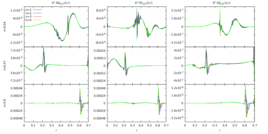
Figure 1: Dispersion with slow rotation: Plots of $4^{n}\delta{\bf\bar{q}}_{h\over 2^{n}}$ against $r$, at four resolutions $n=1,2,3,4$. From the left, the columns represent $\Omega$, $Y$ and $Z$, respectively, while the rows represent the times $t=0.04$, $0.47$ and $0.90$, from the top. In each plot, the curves representing different resolutions approximately align, demonstrating pointwise second-order convergence. The unsmooth but convergent features of the error are artifacts of the MC limiter, and do not correspond to any visible unsmoothness of the solution itself. They are absent with the centered limiter.

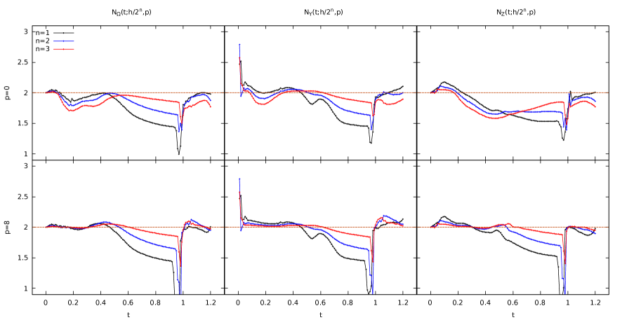
Figure 2: Dispersion with slow rotation: Plots of the convergence rates in the $\ell^{2}$-norm, $\mathcal{N}_{\bf\bar{q}}(t;{h\over 2^{n}},0)$ (upper row, all grid points used) and $\mathcal{N}_{\bf\bar{q}}(t;{h\over n},8)$ (bottom row, last 8 grid points omitted in the norm), for $n=1,2,3$. As in the previous figure the three columns represent $\Omega$, $Y$ and $Z$, respectively. The dashed horizontal line corresponds to second-order convergence, $\mathcal{N}=2$. When the full grid is taken into account in the computation of the norm, we typically observe less than second-order convergence. On the other hand, second-order convergence is recovered once the last 8 grid points are neglected in the computation of the norm.

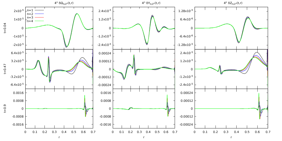
Figure 3: Dispersion with rapid rotation: Note that the instabilities in Fig. 2 at time $t=0.04$ are not present here due to choosing a centered limiter instead of the MC limiter. Otherwise as in Fig. 1.

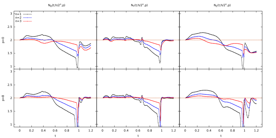
Figure 4: Dispersion with rapid rotation: Otherwise as in Fig. 2.

In Fig. 1, we plot $4^{n}\delta{\bf\bar{q}}_{h\over 2^{n}}$ (left, middle and right columns for $\Omega$, $Y$ and $Z$, respectively) at four different resolutions $n=1,2,3,4$ for initial data that disperses with small angular momentum. The profiles are plotted at three different times (top, middle and bottom rows) $t=0.04,0.36$ and $0.9$. These snapshots represent respectively, the evolution of the error near the initial time, when the energy density reaches a maximum (near the center), and when the matter finally disperses and most of the density is about to leave the numerical domain. During the evolution, the conserved variables remain smooth.

According to (123), the approximate alignment of these plots shows that the code converges to second order. One can, however, spot some instabilities at isolated points inside the numerical grid. Their frequency increases with resolution, but their amplitudes do not grow with time and in fact converge away rather quickly with increased resolution. These instabilities are a consequence of our choice of limiter as we observed that these instabilities vanish with a centered limiter.

On the other hand, the convergence is mostly unaffected by the choice of imposing copy boundary conditions on the conserved variables instead of the primitive or generic variables. Finally, as anticipated, we lose second-order convergence at and near the outer boundary. The error propagates very slowly inside the numerical domain and so does not spoil the second-order convergence for most of the numerical grid for the period of time the simulation is run.

To illustrate this, in Fig. 2 we plot $\mathcal{N}_{\bf\bar{q}}(t;{h\over 2^{n}},0)$ and $\mathcal{N}_{\bf\bar{q}}(t;{h\over 2^{n}},8)$, for $n=1,2,3$. For the former, untruncated case, we find that the order of convergence is typically less than second order. On the other hand, we recover the expected second-order accuracy once the last 8 grid points are ignored in the calculation of the norm. The drop in convergence that can be seen at around $t\simeq 1.0$ corresponds to the energy leaving the numerical grid, see the last row of Fig. 1.

In Figs. 3 and 4, we demonstrate second-order convergence pointwise and with respect to the $\ell^{2}$ norm for the highly rotating dispersing initial data. As for the slowly rotating case, the conserved variables remain smooth during the evolution.

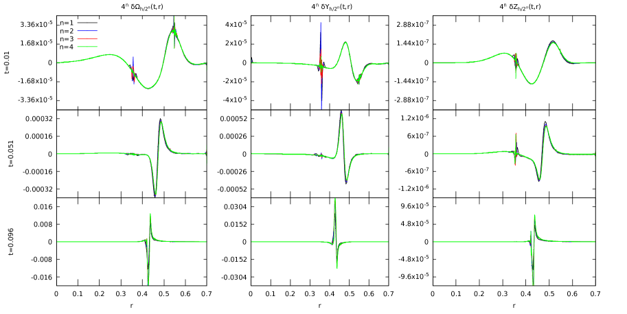
Figure 5: Collapse with slow rotation: Times are now $t=0.010$, $0.051$ and $0.096$ (rows, from top to bottom), otherwise as in Fig. 1.

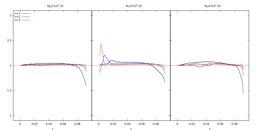
Figure 6: Collapse with slow rotation: Plots of $\mathcal{N}_{\bf\bar{q}}(t;{h\over 2^{n}},0)$, for $n=1,2,3$. As always, the columns correspond to $\Omega$, $Y$ and $Z$ from left to right. Due to the prompt collapse, second-order convergence is maintained throughout the evolution.

Figure 7: Collapse with rapid rotation: Times are now $t=0.010$, $0.130$ and $0.264$, otherwise as in Fig. 5. Note that we lose second-order convergence at the onset of collapse and near the region of black hole formation.

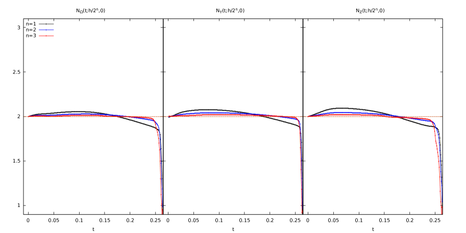
Figure 8: Collapse with rapid rotation: Otherwise as in Fig. 6. Second-order convergence is lost near the onset of collapse, as seen also in the last row (time) of Fig. 7.

Turning our attention now to the collapse case, in Fig. 5 we show $4^{n}\delta{\bf\bar{q}}_{h\over 2^{n}}$ at four different resolutions $n=1,2,3,4$ at times $t=0.01,0.051$ and $0.096$. We find the same qualitative behavior as for the dispersion case, except that the outer boundary behaves much better.

As a consequence, in Fig. 6, we only plot $\mathcal{N}_{\bf\bar{q}}(t;{h\over 2^{n}},0)$ as we have good second-order convergence without the need to truncate the grid. As for dispersion, the choice of limiter and which variables the outer boundary conditions are applied to do not produce any qualitative differences, except for the centered limiter which removes the instabilities already noted in the dispersion case, see Fig. 5.

Finally, in Figs. 7 and 8, we demonstrate second-order convergence for the case of rapidly rotating collapsing data. As one would expect, the presence of angular momentum delays the time of collapse. Near the onset of collapse the convergence drops to first-order near the region where the horizon forms.

V.3 Stable and unstable stars

In [6], we analysed in detail the family of stationary solutions parametrized by two dimensionless constants, $(\Omega_{0},\mu)$ or equivalently $(\tilde{J},M)$, where we defined the dimensionless spin

$$\tilde{J}:={J\over\ell}.$$ (129)

In the parameter space $(\Omega_{0},\mu)$, it was shown that the set of parameters which result in a solution that is regular everywhere and asymptotes to a BTZ solution with $\tilde{J}\leq M$ is doubly covered for each admissible pair of values $(\tilde{J},M)$. Both regions are separated by a curve on which solutions have a zero mode, i.e. a static linear perturbation that corresponds to an infinitesimal change in $(\Omega_{0},\mu)$ that leaves $(\tilde{J},M)$ invariant to linear order.

Such a double cover is familiar in $3+1$ dimensions, where the less dense star is stable and the more dense star unstable. Analogously, it was conjectured that the solution with the smaller $\mu$ associated to a given $(\tilde{J},M)$ is unstable, while the one with the larger $\mu$ is stable. We use this opportunity to provide some numerical evidence for this claim. Specifically, consider the pair of solutions with total mass and angular momentum given by $\tilde{J}=0.24,M=0.38$, corresponding to $(\Omega_{0},\mu)\simeq(0.154,0.242)$ and $(0.153,0.392)$. These correspond to the black and orange dots in Fig. 1 in [6] and therefore to the unstable and stable solutions associated to the above conserved quantities $\tilde{J},M$.

For both the stable and unstable configuration, we add a small Gaussian perturbation, with plus or minus sign. The Gaussian perturbation is of the form (126)-(128), with $|p_{\omega}|=0.001,p_{\eta}=p_{\zeta}=0$, $R_{\omega}=0.4$, $\sigma_{\omega}=0.2$. We set $r_{\text{max}}=0.9$ and consider again five different resolutions, with the lowest resolution now $800$ grid points, or $h\simeq 0.00015$. We choose a larger value of $r_{\text{max}}$ because that the stationary initial data under consideration do not have a surface at some finite area radius. Consequently, one needs to choose a larger value of $r_{\text{max}}$ to fit “most” of the energy density inside the numerical grid. We find that a MC or minmod limiter produces large instabilities in the evolution and that these are mostly tamed with a centered limiter. Furthermore, it is essential to use the primitive variables for the copy boundary conditions. Using the conserved variable instead causes the star to disperse almost immediately due to a perturbation originating from the outer boundary, while using the generic variables produces noticeably larger errors during the evolution. We will therefore restrict to this choice in what follows. Lastly, due to the nonvanishing of the conserved variables at the boundary, it is necessary to impose, as for the highly rotating collapse case, that the flux of $\Omega$ be non-negative at the numerical outer boundary. For the stable stationary initial data, we also impose the flux of $Z$ to be positive at the numerical outer boundary. (Note that by construction, $Z$ is non-negative everywhere initially).

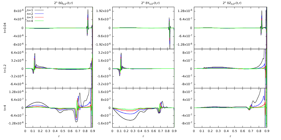
Figure 9: Stable stationary star: Times are now $t=0.04$, $1.2$ and $4$ (rows, from top to bottom). We find $1<\mathcal{N}<2$ inside the numerical grid. The numerical error is dominated by the outer boundary. This error does not converge, but travels inward very slowly and its width shrinks with increased resolution.

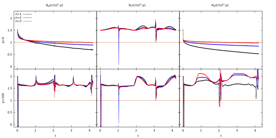
Figure 10: Stable stationary star: Plots of $\mathcal{N}_{\bf\bar{q}}(t;{h\over 2^{n}},0)$ (upper row) and $\mathcal{N}_{\bf\bar{q}}(t;{h\over 2^{n}},100)$ (bottom row), for $n=1,2,3$. The dashed horizontal line corresponds to first-order convergence $\mathcal{N}=1$. When the full grid is taken into account in the computation of the norm, we typically observe first-order convergence. On the other hand, by neglecting the last 100 grid points in the computation of the norm, we observe convergence of about $\mathcal{N}\simeq 1.5$ for $\Omega$ and $Y$ and $\mathcal{N}\simeq 2$ for $Z$.

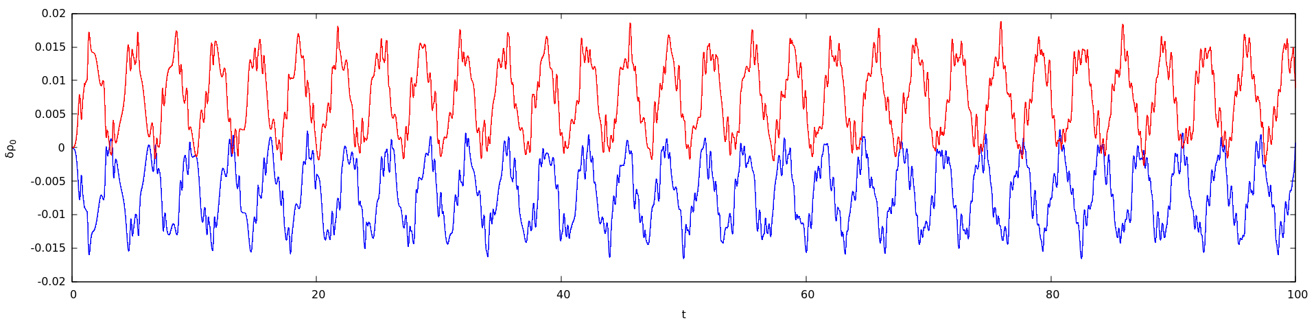
Figure 11: Stable stationary star: Central density perturbation against time for approximately $30$ oscillation periods. Red curve corresponds to the stationary initial data with $p_{\omega}=0.001$ and blue curve with $p_{\omega}=-0.001$.

Let us first consider the stable stationary solution. In Fig. 9, we plot $2^{n}\delta{\bf\bar{q}}_{h\over 2^{n}}$ at four different resolutions $n=1,2,3,4$. These are again plotted at three different times (rows), $t\simeq 0.04,1.2,4.2$. We only show the case $p_{\omega}=-0.001$ as the case where $p_{\omega}=0.001$ is qualitatively similar. Note the different power of $h$ from the dispersion/collapse case, due to the fact that we typically get less than second-order convergence. The cause of this is an instability originating from the outer boundary propagating inwards. At the time $t\simeq 4.2$, this instability has moved to and from the boundary twice. Equivalently, the time for the error originating from the numerical outer boundary to reach the center is $\Delta t\simeq 1.0$. As a consequence, the simulation losses its second-order accuracy everywhere. There is also an instability at and near the outer boundary that does not converge at all, but rather is roughly equal at different resolutions. Nevertheless, as in the case of dispersion, this instability propagates into the numerical grid very slowly and its size shrinks with increased resolution.

In Fig. 10, we plot the convergence in the norm. Due to the combination of the error originating from the outer boundary and the error near the boundary not converging at all, we find $\mathcal{N}_{\bf\bar{q}}(t;{h\over 2^{n}},0)\simeq 1$. Once the region near the outer boundary is neglected by removing the last 100 grid points, we recover approximate second-order convergence $\mathcal{N}_{\bf\bar{q}}(t;{h\over 2^{n}},100)\simeq 2$.

In Fig. 11, we plot the oscillations in the central density, $\delta\rho_{0}(t):=\rho_{0}(t)-\rho_{0}(0)$ for both signs of the perturbation, $p_{\omega}=\pm 0.001$. The simulation is run with $3200$ grid points, for sufficiently long time so that the central density displays approximately $30$ cycles. These oscillations maintain constant small amplitude, proportional to the initial perturbations, and we conjecture that they are essentially linear oscillations with constant frequency, as one would expect in a stable star. The central density oscillates about an average that is offset from the unperturbed star, because our perturbation of the initial data changes the total mass of the star. Our unphysical copy outer boundary condition does not seem to destroy this continuum property. Note that when checking convergence, we only evolve the initial data up to at most $t=4$. The reason is that for convergence testing, we consider much higher resolution than we do in Fig. 11. Compare for example the highest resolution run ($n=5$, equivalent to $25600$ gridpoints) when testing convergence, with the much lower resolution used to produce Fig. 11 ($n=2$, equivalent to $3200$ gridpoints).

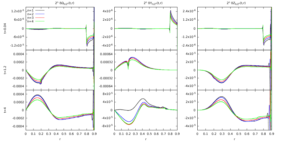
Figure 12: Unstable stationary star with negative density perturbation: A first-order error originating from the outer boundary travels inward, causing the evolution to converge only to first-order. Otherwise as in Fig. 9.

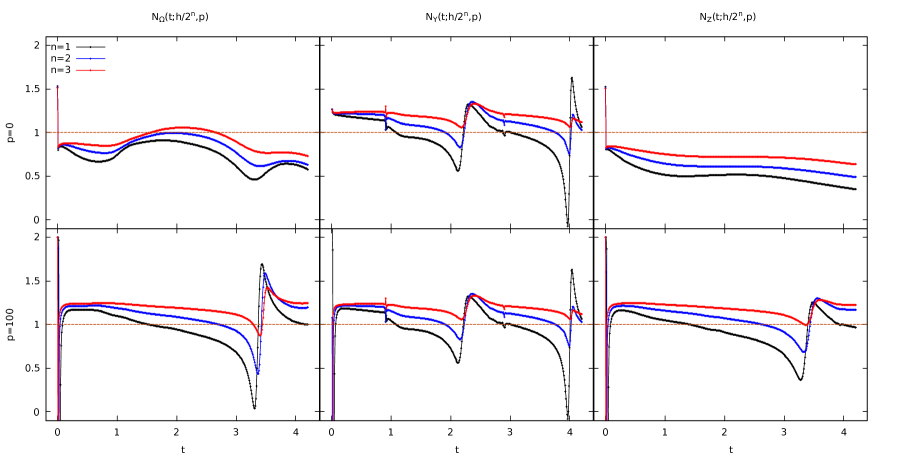
Figure 13: Unstable stationary star with negative density perturbation: Plots of $\mathcal{N}_{\bf\bar{q}}(t;{h\over 2^{n}},0)$ (upper row) and $\mathcal{N}_{\bf\bar{q}}({h\over 2^{n}},100)$ (bottom row), for $n=1,2,3$. The dashed horizontal line corresponds to first-order convergence, $\mathcal{N}=1$. We find first-order convergence once the last 100 grid points are neglected.

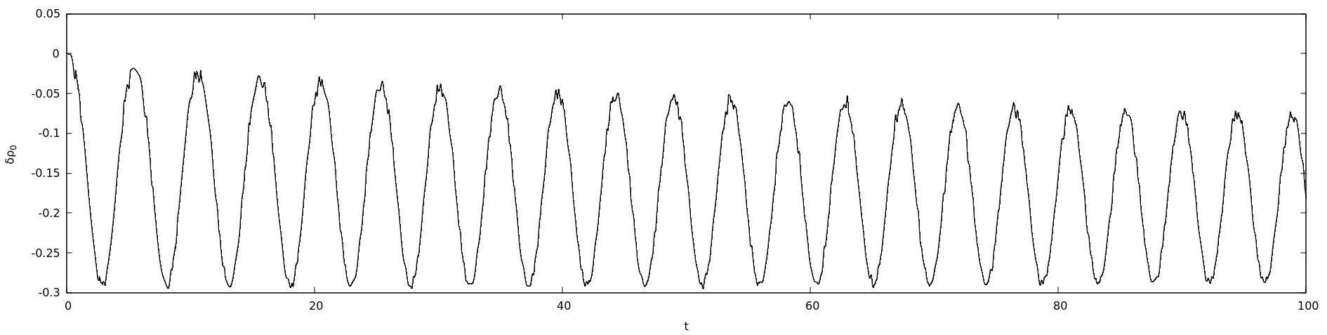
Figure 14: Unstable stationary star with negative density perturbation: Central density perturbation against time. The star breathes nonlinearly without collapsing. Compare with blue curve in Fig. 11.

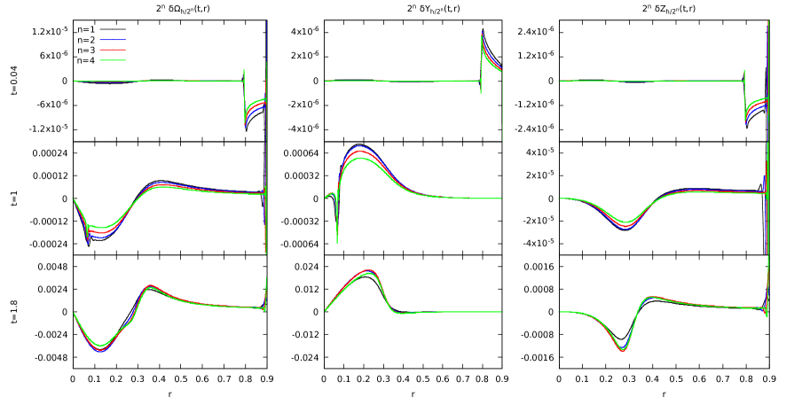
Figure 15: Unstable stationary star with positive density perturbation: We observe qualitatively similar behavior as for Fig. 12.

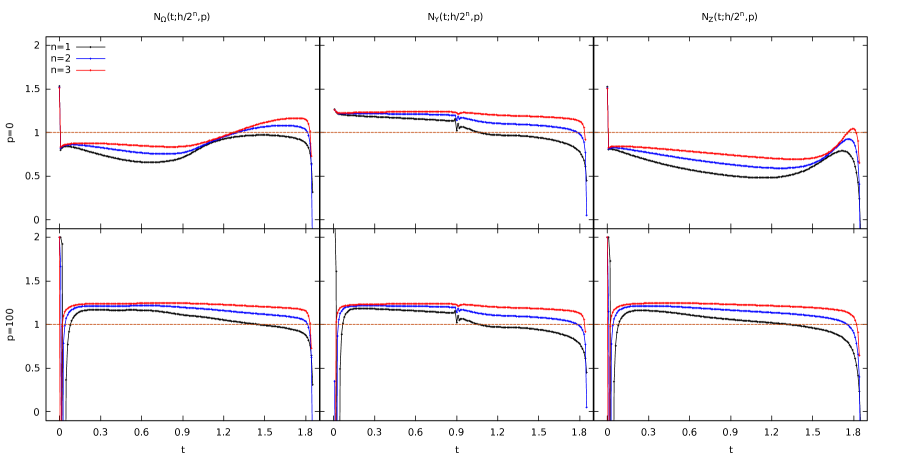
Figure 16: Unstable stationary star with positive density perturbation: Plots of $\mathcal{N}_{\bf\bar{q}}(t;{h\over 2^{n}},0)$ (upper row) and $\mathcal{N}_{\bf\bar{q}}(t;{h\over 2^{n}},100)$ (bottom row), for $n=1,2,3$. The dashed horizontal line corresponds to first-order convergence. We find here fairly constant convergence of $\mathcal{N}_{\bf\bar{q}}(t;{h\over 2^{n}},100)\simeq 1.2$ up until the onset of collapse.

Figure 17: Unstable stationary star with positive density perturbation: We plot the metric coefficient $a(t_{i},r)$ (left) at different times $t_{i}$, ranging from the initial time to the onset of collapse, as well as the central density against time (right). For this (positive) sign of the initial density perturbation, the star promptly collapses. Black-hole formation is triggered due to the timestep becoming small ($\Delta t\sim 10^{-10}$).

Let us now turn to the unstable stationary solution. The convergence tests for both cases are summarized in Figs. 12 and 13 ($p_{\omega}=-0.001$) and Figs. 15 and 16 ($p_{\omega}=0.001$).

Recall that for the unstable configuration, we have not imposed the positivity of the HLL flux for $Z$ at the outer boundary, as we heuristically find that otherwise a small shock forms during the evolution, which prevents the simulation to converge to the desired order in the norm. On the other hand, lifting this constraint on the flux of $Z$ causes a first-order error originating from the outer boundary to propagate inwards. The time for this error to reach the center (for both signs of $p_{\omega}$) is $\Delta t\simeq 0.9$. The simulation is only about first-order accurate.

As for the stable configuration, there is also an instability at and near the outer boundary which does not converge at all, but rather is roughly equal at different resolutions. Nevertheless, this instability propagates into the numerical grid very slowly and its size shrinks with increased resolution. Such a behavior can also be noted for the stable configuration discussed above if the constraint on the positivity of the HLL flux of $Z$ is removed there. In particular, a more careful treatment of the boundary conditions at the numerical outer boundary will be needed to accurately evolve the stationary solutions.

For a positive sign of the initial density perturbation, the star promptly collapses into a black hole, see Fig. 17. On the other hand, for a negative sign, the star does not collapse. Instead, it breathes, i.e. the central density oscillates periodically with very large amplitude, down to about half of the stationary value. This can be seen in Fig. 14, where we plot the central density perturbation $\delta\rho_{0}(t)$ at sufficiently long times for $30$ cycles. The simulation is run with $3200$ grid points as well. The local maxima stay approximately constant throughout the simulation, and the central density is approximately periodic.

It should be again emphasized that due to the fluctuating numerical convergence for the stable and oscillating unstable cases (see again Figs. 10 and 13), it is uncertain how much of Fig. 11 and Fig. 14 is physical or a numerical effect. Nonetheless, we can already observe qualitative differences in the evolution between the stable and unstable stationary initial data even at short times.

VI Conclusions

In this paper, we have presented a new code to simulate the Einstein-fluid equations in axisymmetry in $2+1$ dimensions. We have focused on the ultrarelativistic equation of state $p=\kappa\rho$. However it should be straightforward to adapt the code to an arbitrary barotropic or hot equation of state.

In the case of generic initial data that disperse or collapse both with small and large angular momenta, we have demonstrated that the code converges to second order in resolution both pointwise and in the $\ell^{2}$ norm, except at and near the numerical outer boundary, and near the onset of black hole collapse for highly rotating configurations.

We have also evolved stable and unstable rotating stationary stars. For these, the code converges only to first order. Nevertheless, we can clearly distinguish stable and unstable stars, even at short times. The former remain approximately stationary, with only small oscillations, while the latter show two distinct evolutions depending on the sign of the perturbation that we apply it to, either collapse or very large (but still periodic) oscillations. This provides some evidence in favor of our claim in [6], where it was suggested that the family of stationary stars with $|J|\leq M\ell$ is divided into two families of stable and unstable solutions.

A fundamental strength of our approach is that we make full use of the existence of two conserved matter currents (unexpectedly, for energy as well as, expectedly, for angular momentum) and related local expressions for the mass $M$ and angular momentum $J$. As a consequence the metric evolution is fully constrained, and $M$ and $J$ are exactly conserved.

A well-known disadvantage of polar-radial coordinates is that our code stops as an apparent horizon is approached. However, one could in principle make equal use of the two conserved currents and conserved quantities in other coordinates.

The main weakness of our code as presented here is that we have not found a way of extending the outer boundary all the way to the timelike infinity of any asymptotically BTZ spacetime, in a way that is stable and accurate [16]. This means that we have to impose an unphysical “copy” boundary condition at finite radius $R$. Fortunately, it turns out that, with some fine-tuning, this does not prevent us from carrying out long-term (many sound-crossing times) evolutions of stars. Moreover, it also does not seem to be an obstacle in the investigation of critical phenomena at the threshold of (prompt) collapse, which we will report on in a companion paper.

- [1] M. Bañados, C. Teitelboim and J. Zanelli, Black Hole in Three-Dimensional Spacetime, Phys. Rev. Lett. 69, 13 (1992).
- [2] H. Kodama, Conserved energy flux for the spherically symmetric system and the backreaction problem in the black hole evaporation, Prog. Theor. Phys. 63, 1217 (1980).
- [3] H. Maeda and M. Nozawa, Generalized Misner-Sharp quasi-local mass in Einstein-Gauss-Bonnet gravity, Phys. Rev. D 77, 064031 (2008).
- [4] S. Kinoshita, Extension of Kodama vector and quasilocal quantities in three-dimensional axisymmetric spacetimes, Phys. Rev. D 103, 124042 (2021).
- [5] D.W. Neilsen and M.W. Choptuik, Ultrarelativistic fluid dynamics, Classical Quantum Gravity 17, 733 (2000).
- [6] C. Gundlach and P. Bourg, Rigidly rotating perfect fluid star in dimensions, Phys. Rev. D 102, 084023 (2020).
- [7] M. Cataldo, Rotating perfect fluids in ()-dimensional Einstein gravity, Phys. Rev. D 69, 064015 (2004).
- [8] J. A. Font, Numerical hydrodynamics and magnetohydrodynamics in general relativity, Living Rev. Relativity 11, 7 (2008).
- [9] M. Alcubierre, Introduction to Numerical Relativity (Oxford University Press, New York, 2008).
- [10] P. J. Montero, T. W. Baumgarte and E. Müller, General relativistic hydrodynamics in curvilinear coordinates, Phys. Rev. D 89, 084043 (2014).
- [11] M. W. Choptuik, Universality and Scaling in Gravitational Collapse of a Massless Scalar Field, Phys. Rev. Lett. 70, 9 (1993).
- [12] M. Bañados, M. Henneaux, C. Teitelboim, and J. Zanelli, Geometry of the black hole, Phys. Rev. D 48, 1506 (1993).
- [13] P. Bizoń and A. Rostworowski, Weakly Turbulent Instability of Anti-de Sitter Spacetime, Phys. Rev. Lett. 107, 031102 (2011).
- [14] B. J. van Leer, Towards the ultimate conservative difference scheme I. The quest of monotonicity, Lect. Notes in Phys. 18, 163 (1973).
- [15] B. Einfeldt, On Godunov-type methods for gas dynamics, SIAM J. Numer. Anal. 25, 294 (1988).
- [16] P. Bourg, Critical phenomena in gravitational collapse, Ph.D thesis (unpublished).
- [17] R. J. Leveque, Finite Volume Methods for Hyperbolic Problems (Cambridge University Press, Cambridge, England, 2002), pp. 100-128.