Subaru Hyper Suprime-Cam excavates colossal over- and under-dense structures over 360 deg² out to z = 1

Abstract

Subaru Strategic Program with the Hyper-Suprime Cam (HSC-SSP) has proven to be successful with its extremely-wide area coverage in past years. Taking advantages of this feature, we report initial results from exploration and research of expansive over- and under-dense structures at $z=$ 0.3 – 1 based on the second Public Data Release where optical 5-band photometric data for $\sim$ eight million sources with $i<23$ mag are available over $\sim 360$ square degrees. We not only confirm known superclusters but also find candidates of titanic over- and under-dense regions out to $z=1$. The mock data analysis suggests that the density peaks would involve one or more massive dark matter haloes ($>10^{14}$ M_⊙) of the redshift, and the density troughs tend to be empty of massive haloes over $>10$ comoving Mpc. Besides, the density peaks and troughs at $z\lesssim 0.6$ are in part identified as positive and negative weak lensing signals respectively, in mean tangential shear profiles, showing a good agreement with those inferred from the full-sky weak lensing simulation. The coming extensive spectroscopic surveys will be able to resolve these colossal structures in three-dimensional space. The number density information over the entire survey field is available as grid-point data on the website of the HSC-SSP data release (https://hsc.mtk.nao.ac.jp/ssp/data-release/).

1 Introduction

Mapping large-scale structures on cosmological scales and studying properties of galaxies therein across the cosmic time inform us of the role of large-scale environment on galaxy evolution in the hierarchical universe. In the local universe, more than a dozen studies and discussions have been made on the environmental dependence of galaxy evolution over such an extensive survey volume (Tanaka et al., 2004; Baldry et al., 2006; Sorrentino et al., 2006; Park et al., 2007; Peng et al., 2010; Alpaslan et al., 2015; Douglass & Vogeley, 2017), based on data such as the Sloan Digital Sky Survey (York et al., 2000; Eisenstein et al., 2011; Blanton et al., 2017), the 2dF Galaxy Redshift Survey (Colless et al., 2001), and the Galaxy And Mass Assembly survey (Driver et al., 2009, 2011; Liske et al., 2015). Beyond the local universe, on the other hand, such efforts remain far from complete due to the lack of deep and extremely wide-field data.

Meanwhile, statistics of cosmic voids have been gaining a lot of attention in constraining cosmological parameters such as density contrast, dark energy parameter, and neutrino mass (Regos & Geller, 1991; Dekel & Rees, 1994; Agarwal & Feldman, 2011; Pisani et al., 2015; Contarini et al., 2019), and to test modified gravity (Clampitt et al., 2013; Cai et al., 2015). Supervoids are considered to be a causal factor of a controversial feature seen in the cosmic microwave background, namely the so-called "cold spot" (Inoue & Silk, 2006, 2007; Szapudi et al., 2015; Finelli et al., 2016). Such diffuse environments also provide us with galaxy growth driven by in-situ process (Peebles, 2001; Rojas et al., 2005). However, it has been challenging to exhaustively investigate void galaxies beyond the local universe until recently as such an exploration is too expensive without wide-field imager or spectrograph on large aperture telescopes.

The circumstances prevailing today are no longer the same as in the past, thanks to the advent of wide field imaging surveys over $>100$ square (sq.) deg area, such as the Canada–France–Hawaii Telescope Lensing Survey (Heymans et al., 2012), the Kilo-Degree Survey (de Jong et al., 2013), the Dark Energy Survey (DES) (Abbott et al., 2018), and the Subaru Strategic Program with the Hyper Suprime-Cam (Aihara et al., 2018a). The two-point correlation and power spectrum analyses of cosmic shear have proven successful as a powerful cosmological probe (e.g., Heymans et al. 2013; Hildebrandt et al. 2017; Hikage et al. 2019). More recently, Gruen et al. (2018) demonstrate cosmological constraints from the density contrast over the wide-field area by measuring galaxy number densities and gravitational lens shears based on DES First Year and SDSS data. Nevertheless, a number of scientific questions related to galaxy evolution still remain unanswered; the millions of galaxies from the aforementioned surveys thus provide us with wonderful data for more detailed investigations.

Subaru Strategic Program (SSP) with the Hyper Suprime-Cam (HSC), the prime focus camera on the Subaru Telescope with an exceptionally wide-field view (1.5 deg in diameter) compared to other 8-meter class telescopes began in 2014 (Miyazaki et al., 2018; Furusawa et al., 2018; Kawanomoto et al., 2018; Komiyama et al., 2018). The program has now completed $\sim 90$ per cent of the allocated observing runs, reaching $\sim$1,000 sq. degrees as of this writing. HSC-SSP is designed to address a various range of fundamental questions such as weak-lensing cosmology and galaxy evolution out to the early Universe. Such in-depth, wide-field data enable systematic explorations and surveys of unique large-scale systems out to high redshifts (see, e.g. a red-sequence cluster search at $z=$ 0.1 – 1.1 by Oguri et al. 2018; a protocluster search at $z\sim 4$ by Toshikawa et al. 2018). The high quality and large-volume data-set taken from the 8-meter class telescope permits statistical research of galaxy properties such as mass assembly histories and red fractions of galaxies in galaxy clusters (Lin et al., 2017; Nishizawa et al., 2018) and a morphological classification (Tadaki et al., 2020) for more than ten thousands or millions of sources.

We thus started working on density mapping at $z>0.3$ on the cosmological scale to discover the very-large over- and under-dense structures like superclusters and cosmic voids (de Vaucouleurs, 1953; Gregory & Thompson, 1978; Kirshner et al., 1981; Oort, 1983), and also on comprehensive analyses of galaxy characteristics as a function of the large-scale environments across the cosmic time. This paper reports initial results from our systematic search for gigantic over- and under-dense structures with HSC-SSP. As the first in a series of papers stemmed from our research, we focus on the density mapping over $\sim 360$ square (sq.) degrees where the data are publicly accessible, which is less than one-third of the $\sim 1,400$ sq. degrees to be covered at the end of the program. We overview the data-set in §2, and then, explain the density estimation and present resultant maps (§3). The discussion part (§4) evaluates total masses associated with discovered colossal over- and under- densities based on a mock galaxy catalogue from a sizeable cosmological simulation and a weak lensing analysis. Lastly, we summarise highlights of this work and remark about the outlook for upcoming related programs (§5). Throughout the paper, we adopt the AB magnitude system (Oke & Gunn, 1983), and cosmological parameters of $\Omega_{M}=0.279$, $\Omega_{\Lambda}=0.721$, and $h=0.7$ in a flat Lambda cold dark matter model that are consistent with those from the WMAP nine year data (Hinshaw et al., 2013). When we refer to figures or tables shown in this paper, we designate their initials by capital letters (e.g., Fig. 1 or Table 1) to avoid confusion with those in the literature.

2 HSC-SSP catalogue

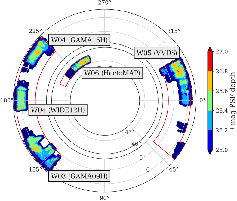
Figure 1: The above shows the sky coverage in PDR2 where colour-code means five sigma PSF limiting magnitude in two arcsec diameter at $i$-band. We cut out five areas as denoted on the sky map. The red rectangle area indicates the survey footprint of HSC-SSP (Aihara et al., 2018a).

This work is based on the second Public Data Release (PDR2) of HSC-SSP, which became public on 2019 May 30 (Aihara et al., 2019). The HSC-SSP PDR2 contains the data taken during March 2014 and January 2018. The detailed information about PDR2 is summarised by Aihara et al. (2019, table 2). The database provides us with the science-ready catalogue through the data processing by the dedicated pipeline called hscPipe (Bosch et al., 2018). We first collect bright sources in the $i$-band ($<23$ mag) with more than five sigma detection in cmodel measurement in all HSC bands at 0.4 – 1.1 $\mu$m ($g/r/i/z/y$). As for the cmodel measurements, we refer readers to Bosch et al. (2018, §4.9.9). We here exclude sources near bright stars ($<17.5$ mag), and those affected by cosmic rays, bad pixels, or saturated pixels using the following flags on the HSC-SSP database: pixelflags_edge, pixelflags_interpolatedcenter, pixelflags_saturatedcenter, pixelflags_crcenter, pixelflags_bad, pixelflags_bright_objectcenter, and mask_s18a_bright_objectcenter (Coupon et al. 2018; Aihara et al. 2019; Bosch et al. 2018, table 2).

We employ an area totally $\sim 360$ sq. degrees from the available HSC-SSP Wide layer (Aihara et al. 2019, figure 1; see also Fig. 1) in which five sigma limiting magnitude of point-spread-function (PSF) in two arcsec diameter is deeper than 26 mag in $i$-band. These criteria are chosen to prevent the need for correction of the variance of number densities due to depth variation across the survey field (see Fig. 2, 3 and a detailed description in §3.1). One should note that we exclude two fields, W01 (WIDE01H) and W02 (XMM) regions (Aihara et al., 2019), which cover much narrower areas than the other fields (W03–W06) in the PDR2 database. After that, we select samples in a photometric redshift (photo-$z$) range from $z=$ 0.3 to 1 using Mizuki, an SED-based photo-$z$ code (Tanaka, 2015). The biweight dispersion of $\Delta z=|z_{\mathrm{spec}}-z_{\mathrm{photo}}|$ and the outlier rate ($|\Delta z|>0.15$) for the HSC sample at $i<23$ mag are $\leq 0.04$ and $\sim 0.1$, respectively (Tanaka et al., 2018, table 2). We only employ objects with the reduced chi-square $\chi_{\nu}<5$ of the best-fitting model following the suggestion in the literature (Tanaka et al., 2018, §7). We carry out a further selection cut for the redshift $z=$ 0.4 – 0.5 bin where there is a strong Balmer–Lyman break degeneracy. Since misclassified objects at $z\sim 3$ tend to show very young ages ($\sim 1$ Gyr) with high specific star-formation rates (SSFRs), we omit such samples which have SSFRs higher than 1 Gyr^-1 to minimise the potential contaminants of Lyman break galaxies at $z\sim 3$. We note that the contamination of Lyman break galaxies for higher redshift bins, such as $i$-band dropouts, is negligible given our detection criteria in all HSC bands, including $g$-band. Through these criteria, our galaxy sample contains about ten million objects.

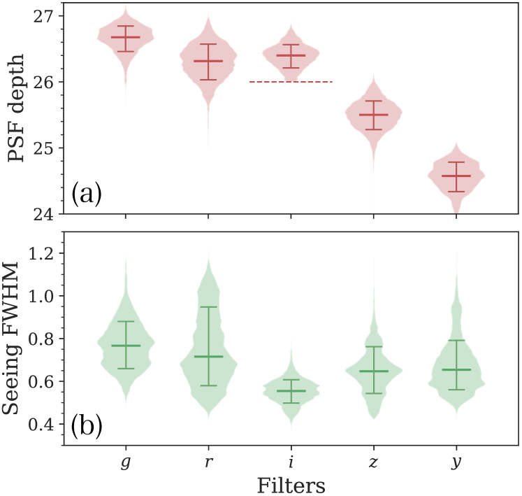
Figure 2: Violin plots of (a) the image depth and (b) the seeing size distributions in $g/r/i/z/y$ broadband filters of HSC. The width of each violin is scaled based on the Gaussian kernel density estimation (KDE). We employ the survey field in which the PSF limiting magnitude in $i$-band is deeper than 26 mag (the dashed line). The horizontal lines in each distribution show the median value and the intervals of 68th percentile.

3 Mapping over- and under-densities

3.1 Density estimation

We count the galaxy number within a top-hat aperture of $r=$ 10 and 30 arcmin ($n_{r=10^{\prime}}$ and $n_{r=30^{\prime}}$) at seven projected redshift slices: $z=$ [0.3:0.4), [0.4:0.5), [0.5:0.6), [0.6:0.7), [0.7:0.8), [0.8:0.9), and [0.9:1.0). A spatial resolution of the projected density map is set to be about 1.5 arcmin that is sufficiently smaller than the aperture sizes. The aperture radius corresponds to 4.0, 5.0, 6.0, 6.9, 7.8, 8.6, 9.4 comoving Mpc (cMpc) in $r=10$ arcmin and 12.1, 15.1, 18.0, 20.8, 23.4, 25.8, 28.1 cMpc in $r=30$ arcmin at $z=$ 0.35, 0.45, 0.55, 0.65, 0.75, 0.85, 0.95, respectively. As a benchmark study of the series of papers, we choose these fixed aperture radii by referencing to those typically used in the Dark Energy Survey (Gruen et al., 2016, 2018). Since this work focuses on enormously large structures ($\gtrsim 20$ cMpc) rather than local (sub-)structures, recent sophisticated density estimations (e.g., Sousbie 2011; Lemaux et al. 2017) are not crucial. Furthermore, the choice of the fixed angular aperture is motivated to provide functional usability with catalogue users. Since our density map catalogue includes the number densities within the fixed apertures at narrower redshift bins ($\Delta z=0.02$), users can reconstruct density maps at a specific redshift space between $z=0.3$ and 1 (Appendix A). Besides, we prefer to use the fixed angular aperture method to keep consistency of a number density correction around holes by bright-star masks and boundaries across redshifts and fields as mentioned below. However, the density catalogue also contains physical aperture measurements of $r=10$ co-Mpc given the use for more scientific purpose, which provide complementary information to the fixed angular aperture estimations.

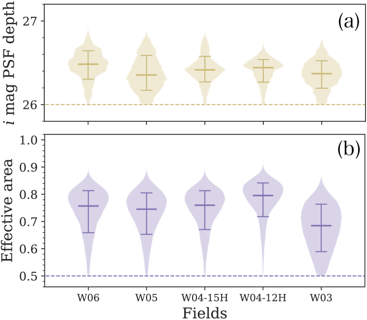
Figure 3: Violin plots for the field variation of (a) the $i$-band limiting magnitude and (b) the effective area, i.e., the fraction of unmasked area. As in Figure 2, the median and 68th percentile values are shown in each bin.

Deriving proper number densities across the entire survey field must need appropriate bright-star masking to determine the effective survey area. For that reason, we implement the random catalogue provided by PDR2, which allows us to evaluate the fraction occupied by the bright-star masks and the boundaries of survey fields in each aperture area for the density estimate (Coupon et al., 2018; Aihara et al., 2019). This work employs only the survey areas that are masked less than 50 per cent at the corresponding grid point. We then apply the mask correction by dividing number densities by unmasked fraction (defined as effective area) to obtain the absolute number densities in each aperture area. One should note that we confirm no clear trend in the median values of mask-corrected number densities toward the effective area, meaning that the mask correction is not systematically over-estimated nor under-estimated. The derived number density distributions in the seven redshift slices with two aperture sizes are summarised in Figure 4. The area of the five fields employed amounts to 359.5 sq. deg in $r=10$ arcmin aperture measurement (or 261.2 sq. deg of the effective area used in the actual calculation; see Table 1), which is the most extensive ever with such a deep optical multi-band photometry. The total number of $i$-band selected sources associated with the whole survey area reaches 7.8 million. Future papers will delve into those characteristics with respect to various cosmic environments.

As a sanity check, we see if the net number densities combined in all redshift bins from $z=0.3$ to 1 have any systematic bias depending on image depth or seeing size in each broadband filter (Fig. 2 and 3). We here adopt the number densities within $r=10$ arcmin apertures which is more comparable to the size of individual HSC patch ($\sim 12\times 12$ arcmin²; see Aihara et al. 2018a, §4) than that with $r=30$ arcmin apertures. Then, we confirm that they are constant relative to various image depths and seeing sizes within the margin of error of less than five per cent (Fig. 5).

Table 1: Map information. The first and second columns are the field id and name. The third and fourth columns show the survey area and the number of density grids where we calculate the number count of targets, which include the outer edges of the survey fields that we do not employ in the analyses. The spatial resolution is about 1.5 arcmin. These columns may be helpful for ones who use the online catalogue (Appendix A). The fifth column indicates the actual survey area satisfying our data requirements and the values in parentheses are the effective field coverage with the effective area $>50$ per cent in $r=10$ arcmin apertures (which are marginally larger in $r=30$ arcmin).

ID	Field	$\alpha_{min}$: $\alpha_{max}$	N grids	Area deg2
		$\delta_{min}$: $\delta_{max}$		(effective)
1	W06 HectoMAP	$\alpha$=224.0:250.0	754$\times$120	38.2
		$\delta$=42.0:45.0		(28.2)
2	W05 VVDS	$\alpha=$330.0:363.0	1320$\times$200	109.4
		$\delta$=$-$1.0:4.0		(80.0)
3	W04 GAMA15H	$\alpha$=206.0:226.0	800$\times$160	56.6
		$\delta$=$-$2.0:2.0		(42.2)
4	W04 GAMA12H	$\alpha$=173.0:190.0	680$\times$160	52.4
		$\delta$=$-$2.0:2.0		(40.8)
5	W03 GAMA09H	$\alpha$=128.0:154.0	1040$\times$260	103.0
		$\delta$=$-$2.0:4.5		(69.9)

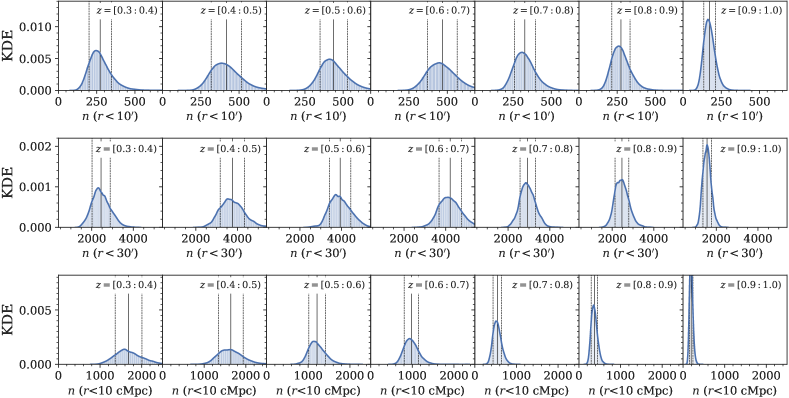
Figure 4: The number density distribution (per aperture) in Gaussian kernel density estimation (KDE) at each redshift range from $z=0.3$ to 1. Those in upper and lower panels respectively show the number of $i$-band magnitude limited ($i<23$) sources within $r=10$ and $r=30$ arcmin apertures. The black solid and dashed lines mean the average and $\pm 1\sigma$ standard deviations for each panel. Here the mask correction has been implemented.

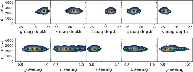
Figure 5: Distributions of the net number densities given by summing all number densities in the seven redshift slices at $z=$ 0.3 – 1 in each aperture, as a function of five sigma limiting magnitude (upper panels) and seeing sizes (lower panels) in $g/r/i/z/y$ bands. The green squares show the median values within small bins of the depth ($\Delta=0.2$ mag) and the seeing size ($\Delta=0.05$ arcsec).

3.2 Projected density map

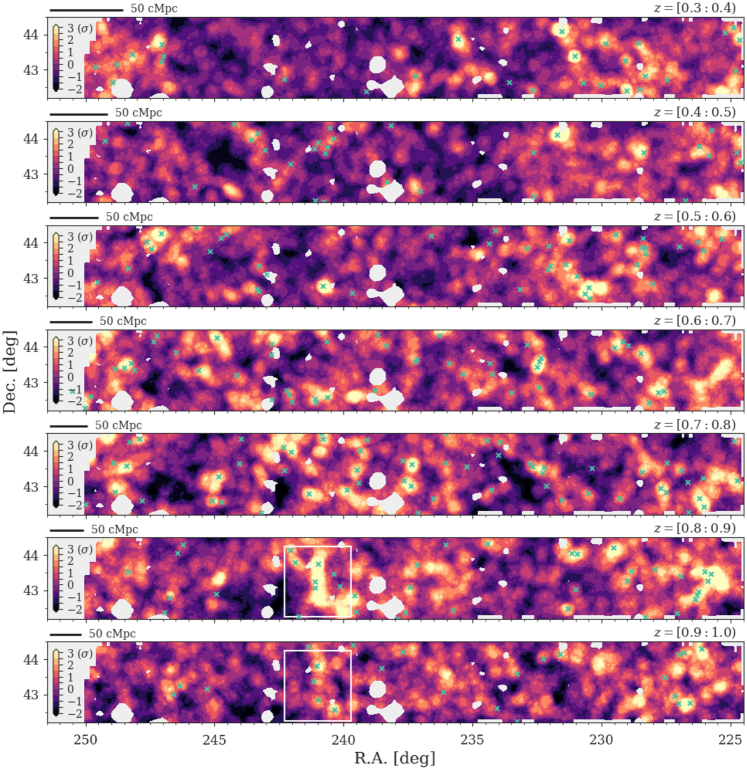
Figure 6: Density maps in W06 (HectoMAP) at $z=$ 0.3 – 1 in step with $\Delta z=0.1$ from top to bottom. Colours indicate the number densities within $r=10$ arcmin in standard deviation ($\sigma$=[$-2$: $+3$]) as denoted in left colour-bars. The eggshell white area is the masked region with effective area of $\leq 50$ per cent. The green crosses show the CAMIRA cluster samples with richness $\geq 15$ at each redshift (Oguri et al. 2018 including the incremental update based on the HSC-SSP PDR2). Density maps for the other fields are available as additional figures through the online journal. The white boxed areas at $z=$ 0.8 – 1.0 locate the whole structure surrounding the CL1604 supercluster (Hayashi et al., 2019).

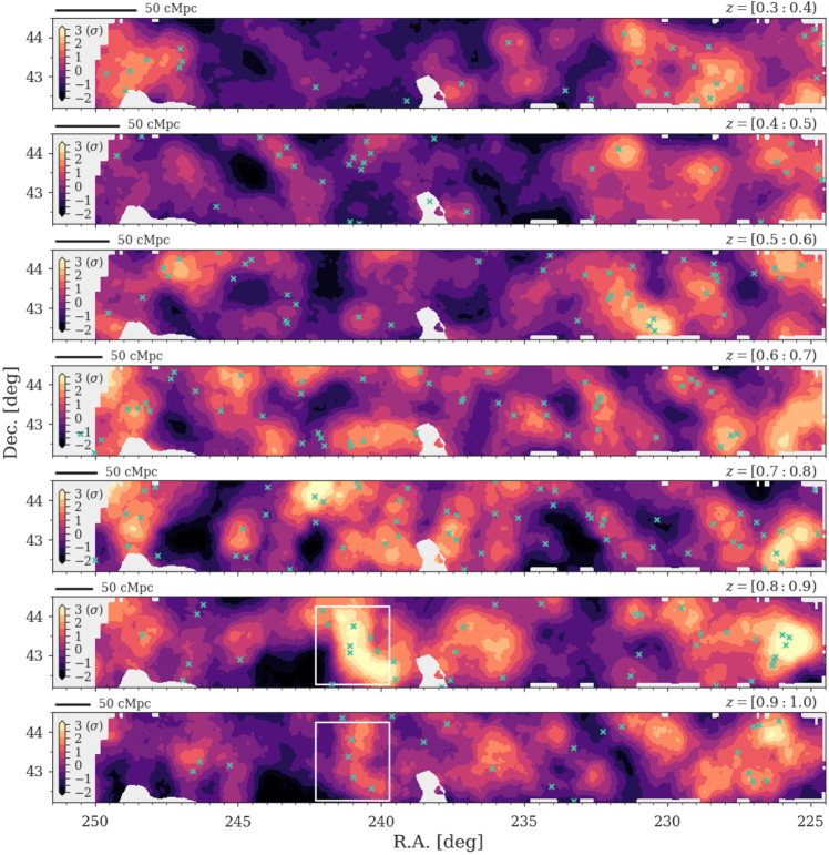
Figure 7: Same as Figure 6 but the number densities within $r=30$ arcmin.

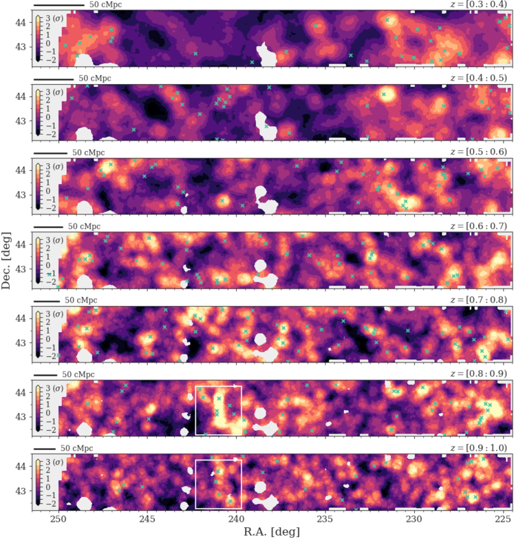
Figure 8: Same as Figure 6 but the number densities within $r=10$ cMpc.

Figure 6 and 7 show the resultant density maps for one of five fields (W06), which largely overlaps with the HectoMAP region (Geller et al., 2011; Geller & Hwang, 2015). The maps are colour-coded by the standard deviation ($\sigma$) to the entire number density distribution (i.e., in all five survey fields) at each redshift (Fig. 4). The area where a mask fraction is higher than 50 per cent is fully masked and is not taken into account in the following analyses. Density maps for the other fields can be found as additional figures through the online journal. Also, grid-point data of the density maps shown in this paper are available online (see Appendix A for details).

We mark positions of galaxy clusters identified by Oguri et al. (2018) based on the CAMIRA algorithm (Oguri, 2014) to cross-check our density measurement with an existing catalogue. One should note that our density estimate is largely different from their selection technique: Oguri et al. (2018) searched for galaxy clusters based on luminous red galaxies within a radius $\lesssim 1$ physical Mpc at more flexible redshift spaces. On the other hand, we calculate number densities in much larger volumes at fixed redshift ranges. In general, none the less, the over-densities in Figure 6-8 show a good agreement with distributions of the CAMIRA clusters. Interestingly, the CAMIRA clusters seem to trace the large-scale structures shown by the projected density maps of this work. For reference, 66 (or 36) and 47 (or 20) per cent of the CAMIRA clusters with richness $>15$ (see Oguri 2014 about the definition) are embedded in $>1$ sigma (or $>2$ sigma) densities of $r=10$ arcmin aperture estimation at $z=$ 0.3 – 0.4 and $z=$ 0.9 – 1, respectively. More mismatch seen at higher redshifts would be mainly due to the larger physical aperture sizes at higher redshift bins in our density calculation since we confirm that the fractions increase when choosing smaller aperture sizes. It may also be affected by photo-$z$ uncertainties and/or fragmentation of massive systems in the earlier universe.

A phenomenal structure seen at $z=$ 0.8 – 0.9 ($\alpha=241^{\circ}$, $\delta=43^{\circ}$) is the CL1604 supercluster (Gunn et al., 1986; Lubin et al., 2000; Gal et al., 2008). A more panoramic picture of this supercluster reaching a 50 cMpc scale is recently reported by Hayashi et al. (2019), which is consistent with what is seen in Fig. 6-8. We should note that the redshift projections at $z=$ [0.8:0.9) and [0.9:1.0) as shown in the figures are somewhat unsuitable for the visualisation of the CL1604 supercluster since they split the whole redshift distribution of CL1604 centring on $z\sim 0.9$ (Gal et al., 2008). Another massive structure appears on the west side at the same redshift, involving six rich CAMIRA clusters. Because of these two enormous structures, the W06 field shows six per cent higher mean number density compared to that of the whole survey area at $z=$ 0.8 – 0.9.

Furthermore, one of those lying at $z=$ 0.8 – 0.9 in W03 GAMA09H ($\alpha=150^{\circ}$, $\delta=2^{\circ}$; Fig. 9) is likely associated with a COSMOS supercluster at $z=$ 0.8 – 0.9 (Paulino-Afonso et al., 2018). We find that about a half of the COSMOS field (Scoville et al., 2007) is covered by $>2$ sigma over-densities in $n_{r=30^{\prime}}$ at $z=$ 0.8 – 0.9. In particular, the western side of the COSMOS supercluster shows the clustering $>4$ sigma density peaks in our photo-$z$ based analysis. This field is out of the survey area by Paulino-Afonso et al. (2018) unfortunately, and thus this large-scale over-dense region is not confirmed yet. A forthcoming deep galaxy evolution survey with Prime Focus Spectrograph (PFS) (Takada et al., 2014) will explore the extended COSMOS region, including this interesting field in the near future.

We detect $\sim 50$ over-densities comparable to such supercluster-embedded regions given seven redshift slices while some of them spatially overlap with each other on the sky. Figure 9 summarises representative examples showing greater than three sigma excesses at the density peaks in the projected density distributions. Spectroscopic follow-up observations are required to confirm these enormous over-densities, though we evaluate their potential mass contents based on the cosmological simulation and the weak lensing analysis in the discussion (§4). The density catalogue available online provides the number densities broken down into $\Delta z=0.02$, allowing more flexible supercluster search (see Appendix A).

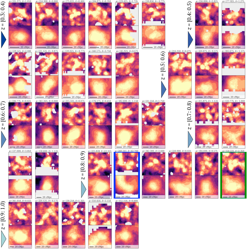
Figure 9: Examples of colossal over-densities at each redshift slice showing the number excess of $>3\sigma$ (roughly corresponding to the density variance of $\delta\gtrsim 0.4$) at the density peak. For each panel of $2\times 2$ sq. deg, upper and lower maps show the density map within $r=10$ and 30 arcmin apertures as in Fig. 6 and 7, respectively. The central coordinates are described on top of each panel. At $z=[0.8,0.9)$, blue and green highlights are associated with the CL1604 and the COSMOS superclusters (Gal et al., 2008; Paulino-Afonso et al., 2018), respectively. The black horizontal bar shown at the bottom of each panel indicates the projected distance of 20 cMpc.

Besides, the continuous wide-field coverage over $\gtrsim 40$ sq. degrees in each field allows us to find widely-spread under-dense structures like cosmic troughs out to $z=1$ as well as over-densities. A cosmic trough is defined as under-dense circles of a fixed radius over a wide redshift slice (Gruen et al., 2016), which is one of promising probes of cosmic voids for the wide-field data. However, the currently available data may remain insufficient to probe supervoids with a scale of $\gtrsim 400$ cMpc (Higuchi & Inoue, 2018) as discussed in relation with the cold spot of the cosmic microwave background (Szapudi et al., 2015; Finelli et al., 2016). High-quality imaging data from the Subaru 8.2m Telescope will provide an important insight into the in-situ dominated galaxy evolution. While studying the environmental dependence of galaxy properties over the survey fields is out of the scope of this paper, the forthcoming paper II will delve into individual galaxies residing in such unique environments.

As a result, we detect a few significant under-densities at each redshift bin, some of which are highlighted in Figure 10. One should note that in Figure 10 we only choose under-dense regions whose density troughs are less affected by the bright-star masks (effective area of $>70$ per cent). The most prominent diffuse structure at $z<0.5$ is found in the W04 GAMA15H field ($\alpha=209.375$, $\delta=0.725$; see in Fig. 10). The density trough shows 2.5 – 2.7 sigma deficit in the density measurement within $r=30$ arcmin apertures, which corresponds to $\delta\sim-0.5$ in the variance of number densities at this redshift range. Here $\delta$ is defined by $(n_{\mathrm{r}}-n_{\mathrm{r,mean}})/n_{\mathrm{r,mean}}$ where $n_{\mathrm{r}}$ is a number density within a radius of 10 arcmin or 30 arcmin, and $n_{\mathrm{r,mean}}$ is the mean value of $n_{\mathrm{r}}$. Intriguingly, the significant under-dense structure persists up to the redshift bin of $z=$ [0.5:0.6), suggesting that the diffuse structure could be of an extent $\sim$1,000 cMpc along the line of sight (see the top left panel in Fig. 10). Another notable under-dense regions is seen in the W05 VVDS field at $z=$ 0.8 – 1 (Fig. 10), which is in part covered by the Deep layer of HSC-SSP. Coming multi-band photometry at 0.3 – 5 $\mu$m in the Deep layer (Aihara et al., 2018a; Sawicki et al., 2019; Moutard et al., 2020; Steinhardt et al., 2014) will enable detailed research in physical properties of galaxies living in such a vastly empty regions.

Since the discovered enormous under-densities are widely spread over the scale of degrees, next-generation wide-field spectrographs are crucially important to obtain better constraints on their properties. The PFS on the Subaru Telescope (Takada et al., 2014) will be able to achieve detailed three-dimensional mapping on cosmological scales in practical observing time, by its extremely-wide area coverage with a field-of-view of 1.38 degree diameter and simultaneous wavelength range at 0.38 – 1.26 $\mu$m. Another solution to confirm these structures may be the convergence maps from weak lensing analyses as recently reported by Davies et al. (2020), though it remains quite challenging to overcome galaxy shape noise on the several $\sim$ tens arcmin scale with the HSC-SSP data. Furthermore, Higuchi & Inoue (2018) have reported that a weak lensing analysis based on the on-going program like HSC-SSP can probe a supervoid at $z\sim 0.2$ with a radius of $\sim 300$ cMpc and a density contrast $\delta\sim-0.3$ at the trough, if such supervoids are present in the survey field. However, the currently available weak lensing data are largely restricted to the survey area of HSC-SSP PDR1, which is more patchy and has much smaller field coverage of 136.9 sq. deg compared to PDR2 and the survey footprints ($\sim$1,400 sq. deg). We thus leave such weak lensing approaches to future work. Instead, this paper carries out the stacking weak lensing analysis, as described in the discussion section (§4.3).

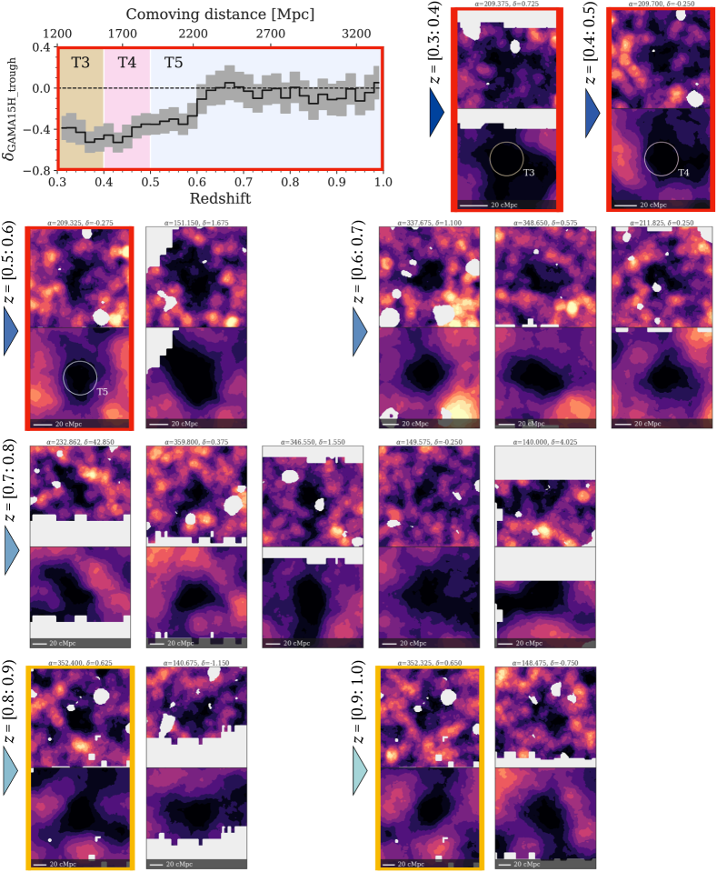
Figure 10: Examples of colossal under-densities at each redshift slice showing $>2.5\sigma$ deficit ($\delta\lesssim-0.3$, $\delta$ is the density variance) at the density trough. Each upper and lower maps are the cutouts of $3\times 3$ sq. deg from the density map within $r=10$ and 30 arcmin apertures as in Fig. 6 and 7, respectively. The central coordinates are denoted on top of each panel. The three under-dense fields at $z=$ [0.3:0.4) framed by red colours are located within the same region on the sky. The upper left figure indicates the density variance at those troughs (T3, T4, T5) as a function of redshift or comoving radial distance. The grey-filled regions show 1 sigma deviations at each redshift bin of $\Delta z=0.02$. The yellow-frame sources at $z=$ 0.8 – 1 in the bottom are covered by the Deep layer of HSC-SSP (Aihara et al., 2018a). The white horizontal bar shown at the bottom of each panel indicates the projected distance of 20 cMpc.

4 Verifying the colossal structures

It is quite important to assess the typical total masses and constrain variance of dark matter densities of the discovered enormous over- and under-dense structures. Such a quantification also works for more practical use of our density map catalogue (Appendix A). In this context, we apply two approaches for the significant over- and under-density regions detected by this work: evaluating massive dark matter haloes associated with the over- and under-densities based on a mock galaxy catalogue from a cosmological simulation (§4.1) and the weak lensing shear measurement (§4.3) to address their underlying masses and densities as in the following sections.

4.1 Mass distribution inferred from the simulation

At first, we specifically consider distributions of massive dark matter haloes across different environments inferred from the projected density map by using the mock galaxy catalogue ($i<23$ mag) from a cosmological simulation. We adopt the data-set from the all-sky gravitational lensing simulation created by Takahashi et al. (2017); Shirasaki et al. (2017). Their simulation data excellently match the scientific motivations of this paper in the following respects: (i) the data cover a sufficiently large cosmological volume, and the area coverage can demonstrate the HSC-SSP Wide layer thanks to the all-sky ray-tracing capability; (ii) the data based on the weak lensing simulation for the HSC-SSP allow us to conduct a cross-comparison of the target regions between the observation and the simulation from the aspects both of galaxy distributions and weak lensing signals (see §4.3).

The details of the full-sky ray-tracing simulation are examined by Takahashi et al. (2017). But we here summarise only the basic parts of the simulation relevant to our analysis. The simulation is based on the $N$-body code, GADGET2 (Springel, 2005) with 14 different boxes with size lengths of 450 – 6300 $h^{-1}$ Mpc in steps of 450 $h^{-1}$ Mpc to create lensing map at different source redshifts (Takahashi et al. 2017, table 1). In each simulation box of $2048^{3}$ particles, they perform six independent realisations with the initial linear power spectrum based on the Code for Anisotropies in the Microwave Background (Lewis et al., 2000, CAMB). The light-ray path and the magnification on the lens planes are derived for 38 different source redshifts from 0 to 5.3 by using the multiple-plane gravitational lensing algorithm GRay-Trix (Hamana & Mellier, 2001; Shirasaki et al., 2015). The particles are positioned on to lens shells with a width of 150 $h^{-1}$ Mpc in the HEALPix coordinates (Gorski et al., 2005). In order to reasonably evaluate the covariances of observables, they select 18 observer’s positions within each simulation box and increase the number of realisations. We refer readers to Shirasaki et al. (2015, appendix C) for more details of the ray-tracing model. The simulation data include a dark matter halo catalogue from the $N$-body simulation using ROCKSTAR (Behroozi et al., 2013) where a halo is defined as a group of more than 50 gravitationally bound particles. The simulation well resolves massive dark matter haloes of virial masses $\gtrsim 10^{13}$ M_⊙ up to $z\sim 1.2$ (Takahashi et al., 2017).

Based on such a large-volume cosmological simulation, we establish one realisation suite specifically designed to mimic the survey field used in this work ($\sim 360$ sq. deg) to check halo distributions surrounding the widely spread over- and under-dense structures. We generate $i$-band magnitude limited sources ($i<23$) at $z=$ 0.3 – 1 from the over-density map of the dark matter particles. To keep consistency with our HSC sample, we adopt the large-scale galaxy bias $b(z)$, which is derived by Nicola et al. (2020, eq. 4.11 and 4.12) based on the HSC PDR1 data (Aihara et al., 2018b). Assuming the linear galaxy bias may not work on the small scale $<10$ cMpc, and thus, this section mainly focuses on the results based on the density estimation with $r=30$ arcmin apertures (corresponding to $r=10$ cMpc at $z=0.3$). Since mock galaxy sources distribute on the celestial sphere corresponding to our survey area, we can conduct the density measurement in the same manner as for the observational data (§3.1). While we do not need to perform the mask correction for the mock data, the edges of the survey fields are removed for the sake of simplifying the calculation. One should note that we here do not consider photo-$z$ uncertainties. However, we stress that photo-$z$ errors, and foreground and background contaminants do not cause a systematic effect on the density measurement but produce some scatters (see a detailed description in Appendix B).

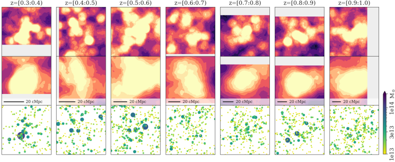
Figure 11: Examples of over-densities in each redshift slice of $\Delta z=0.1$ from $z=$ [0.3:0.4) (the left panels) to $z=$ [0.9:1.0) (the right panels), which are chosen from the projected density map based on the mock catalogue. As in Figure 9, each top and middle maps respectively show the $2\times 2$ deg² cutouts from the density map within $r=10$ and 30 arcmin apertures. Bottom panels show spatial distributions of massive dark matter haloes (M${}_{\mathrm{vir}}>1\times 10^{13}$ M_⊙) within the redshift intervals where colours and sizes of symbols are scaled depending on virial masses of haloes.

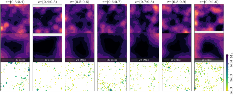
Figure 12: Same as Figure 11 but for under-dense regions.

As in Figure 9 and 10, Figure 11 and  12 respectively highlight some large-scale over- and under-dense regions detected in the ‘mock’ projected density maps. The figures also show spatial distributions of massive dark matter haloes with M${}_{\mathrm{vir}}>1\times 10^{13}$ M_⊙ in each redshift space. These figures demonstrate that significant over-densities are associated with more massive dark matter haloes while the density troughs involve few massive haloes. More statistical tests about halo mass contents appear in Figure 13, which shows the total mass of massive dark matter haloes $>10^{13}$ M_⊙ embedded within $r=30$ arcmin apertures as a function of the number density excess. Positive correlations between the number densities and the total halo masses suggest that our density measurement well traces the large-scale contrasts of halo distributions. Furthermore, the figure suggests that over-dense regions with $\sigma_{r=30^{\prime}}>3$ would host more than 1 – 3 cluster-scale haloes with M${}_{\mathrm{vir}}>1\times 10^{14}$ M_⊙. This is consistent with a picture of superclusters as in the density peaks around the CL1604 and the COSMOS superclusters (§3.2). On the other hand, the mock data suggest about 70 per cent of the density troughs with $\sigma_{r=30^{\prime}}<-2$ do not involve massive haloes with M${}_{\mathrm{vir}}>1\times 10^{13}$ M_⊙ within the range of 30 arcmin at each redshift. Thus, such significant under densities would be good candidates of cosmic voids with radii of $\gtrsim 10$ cMpc (Higuchi et al., 2013).

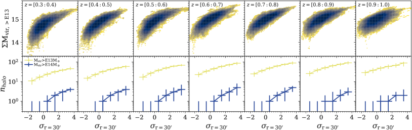
Figure 13: Upper panels indicate total masses of massive dark matter haloes (M${}_{\mathrm{vir}}>1\times 10^{13}$ M_⊙) as a function of the density excess ($\sigma_{r=30^{\prime}}$) within $r=30$ arcmin apertures at $z=0.3$ – 1 in step with $\Delta z=0.1$ from left to right. Lower panels show the number of massive haloes locating within the corresponding apertures of $\Delta z=0.1$ and $r=30$ arcmin in each field. Yellow and blue plots mean the number of massive haloes with M${}_{\mathrm{vir}}>1\times 10^{13}$ M_⊙ and $>1\times 10^{14}$ M_⊙, respectively. Each point and errorbar indicate the median values and 68 percentiles in step with $\Delta\sigma_{r=30^{\prime}}=1$ from $\sigma_{r=30^{\prime}}=-2$ to $\sigma_{r=30^{\prime}}=4$.

4.2 Basics of weak-lensing shear measurement

We then attempt to constrain the typical total masses of discovered over- and under-dense region by employing direct weak lensing measurements. Since it is not realistic to expect any significant detection for individual under-density regions, we adopt a stacking technique (Amendola et al., 1999; Mandelbaum et al., 2006; Okabe et al., 2010; Oguri et al., 2012; Higuchi et al., 2013; Higuchi & Shirasaki, 2016). Before proceeding, we briefly overview the basics of the weak lensing analysis.

An isotropic stretching describes gravitational lensing effects, i.e., convergence $\kappa$ and an anisotropic distortion called cosmic shear $\gamma_{1}$ and $\gamma_{2}$ with the magnification matrix $A$:

$$A_{ij}=\frac{\partial\beta^{i}}{\partial\theta^{j}}\equiv\left(\begin{array}[]{cc}1-\kappa-\gamma_{1}&-\gamma_{2}\\ -\gamma_{2}&1-\kappa+\gamma_{1}\end{array}\right)$$ (1)

where $\theta$ is the lensed angular sky position of a source object and $\beta$ is the un-lensed true position. Practically, the decomposition of the shear field, the tangential distortion $\gamma_{+}$ and the cross distortion $\gamma_{\times}$ components are the only requirements for this work. These are written by the following form,

$$\left(\begin{array}[]{c}\gamma_{+}\\ \gamma_{\times}\end{array}\right)=\left(\begin{array}[]{cc}-\cos 2\eta&-\sin 2\eta\\ -\sin 2\eta&\cos 2\eta\end{array}\right)\left(\begin{array}[]{c}\gamma_{1}\\ \gamma_{2}\end{array}\right)$$ (2)

where $\eta$ is the angle between axis $\alpha$ and $\theta$ on the $\alpha$–$\beta$ plane. The tangential shear becomes positive (negative) when galaxy shape tangentially (radially) deformed with respect to the lens centre. Assuming an axisymmetric lensing profile, the tangential shear contains all the information from lensing, while the cross shear value is ideally zero and thus this can be used to test residual systematic effects. In our stacking analysis, we measure the mean tangential shear profile as a function of radial distances, $\langle\gamma_{+}\rangle$ at radius $\theta_{i}$ from a targeting area (Bartelmann & Schneider, 2001),

$$\langle\gamma_{+}\rangle(\theta_{i})=\tilde{\kappa}(\theta<\theta_{i})-\langle\kappa\rangle(\theta_{i}),$$ (3)

where $\tilde{\kappa}$ is the mean convergence within $\theta_{i}$. The convergence traces the Laplacian of the scalar potential, $\psi(\theta)$ as follows,

$$\begin{split}\kappa(\theta)&=\frac{1}{2}\nabla^{2}\psi(\theta),\\ &=\frac{3H_{0}^{2}\Omega_{M}}{2c^{2}}\frac{D_{ls}D_{l}}{D_{s}a_{l}^{3}}\int\mathrm{d}z\delta(\theta,z),\\ \tilde{\kappa}(\theta<\theta_{i})&=\frac{1}{\pi\theta^{2}}\int_{\theta\leq\theta_{i}}\mathrm{d}\theta^{\prime}\kappa(\theta^{\prime}),\end{split}$$ (4)

where $\delta(\theta,z)$ is the local density fluctuation at the line-of-sight distance $z$ ($\rho(\theta,z)/\tilde{\rho}(z)-1$). $D_{s}$, $D_{l}$ and $D_{l}s$ are the angular diameter distances as described below,

$$D_{s}=a_{s}\chi_{s},\\ D_{l}=a_{l}\chi_{l},\\ D_{ls}=a_{s}(\chi_{s}-\chi_{l}).$$ (5)

$\chi_{s}$ and $\chi_{l}$ are the comoving distance from an observer to source and lens planes, and $a_{s}$ is the scale factor at the source position.

Therefore, measuring the mean tangential shear profile $\langle\gamma_{+}\rangle$ centring on the targets can provide direct insights into their typical density contrast $\delta$ without any knowledge of the galaxy bias. Also, such weak lensing signals give complementary information to what our realistic mocks provide in the previous subsection (§4.1). On top of that, since our mock data from the ray-tracing simulation includes the galaxy shape catalogue for the weak lensing analysis (Shirasaki et al., 2019), we can cross-check results within all these data as discussed in the following section.

4.3 Cross-check with a weak lensing analysis

The weak lensing stacking analysis provides direct insights into the density contrast centred on the target regions. We employ the first-year shear catalogue of HSC-SSP that is available in public. The data cover 136.9 sq. degrees of the HSC-SSP Wide layer taken during March 2014 and April 2016 (Mandelbaum et al., 2018). To test the validation of our weak lensing analysis, we apply the same procedure to the mock galaxy shape catalogue (Shirasaki et al., 2019) which is based on the cosmological weak lensing simulation (Takahashi et al., 2017) introduced in §4.1. While the mock catalogue consists of in total 2,268 realisations of each HSC PDR1 region from 108 full-sky simulation runs with 21 rotations (i.e., $108\times 21=$ 2,268), this work picks up 30 realisations out of 108 full-sky simulation catalogues. Since we are motivated to assess the typical density contrasts and variations around the large over- and under-densities but not aiming for cosmological constraints, 30 realisation data should be enough to check systematic trends and scatters of the lens shear signals for our purpose.

The detailed methodology of the weak lensing stacking is given by Higuchi et al. (2013); Higuchi & Inoue (2019); Higuchi et al. in preparation, while we describe some important notes in our approach below. In the shear measurement, we do not adopt any redshift cut for selecting background galaxies and use all of the galaxies in the shape catalogue. The errors in the shear measurement, such as patchy survey footprints of the HSC survey would generate systematics. To subtract such effects, we subtract lensing signals at random points from the shear profiles for the over- and under-dense regions (Gruen et al., 2016). The errors for the observational results are estimated from the 30 realisations of the mocks (Higuchi et al. in preparation).

The resultant mean tangential shear profiles for both observational and simulation data are presented in Figure 14 and 15. In the stacking analysis, we select the over- and under-dense regions at each redshift slice showing the number excesses of $>3\sigma$ and $<-1.5\sigma$, respectively. The measured mean tangential shear profiles of the observation-based density peaks and troughs are generally consistent with the results from the mocks within the margin of error. However, the signals are too noisy and/or small to obtain meaningful information at $z>0.6$. A more careful redshift selection for background galaxies would be needed to obtain a better signal-to-noise ratio of the lensing profiles at $z>0.6$, but we leave it for future work. Shapes of the detected weak lens profiles also show an agreement with the observational and analytical results obtained in the Dark energy survey (Gruen et al., 2016, 2018).

Ideally speaking, it is expected that over- and under-densities respectively show positive and negative shear signals at $\theta$ corresponding to the aperture radius. Indeed, in the $r=10$ arcmin aperture measurement, the mock results present the signal peaks and troughs around $\theta\sim 10$ arcmin, while the signal strengths become weaker at higher redshift bins (Fig. 14 and 15). The signal detection and the consistency between the observation and the mock data at $z\lesssim 0.6$ suggest that our density estimation well probe analytical over- and under-densities as generated by the cosmological simulation. On the other hand, as inferred from the mock samples, the larger aperture ($r=30$ arcmin) density estimation is less sensitive to the local density contrast than the $r=10$ arcmin aperture, weakening the shear signals which are hardly detected in the current data. Particularly, some outlier signals in the observations (e.g., $\theta\sim 20$ arcmin at $z=[0.4:0.5)$ in Fig. 15) may be due to the limited field coverage of the previous PDR1. The future release of the galaxy shape catalogue for the entire survey footprint ($\sim$1,400 sq. deg) will be able to improve signal-to-noise ratios by a factor of $\sim 3$, allowing better constraints on the weak lensing shear profiles.

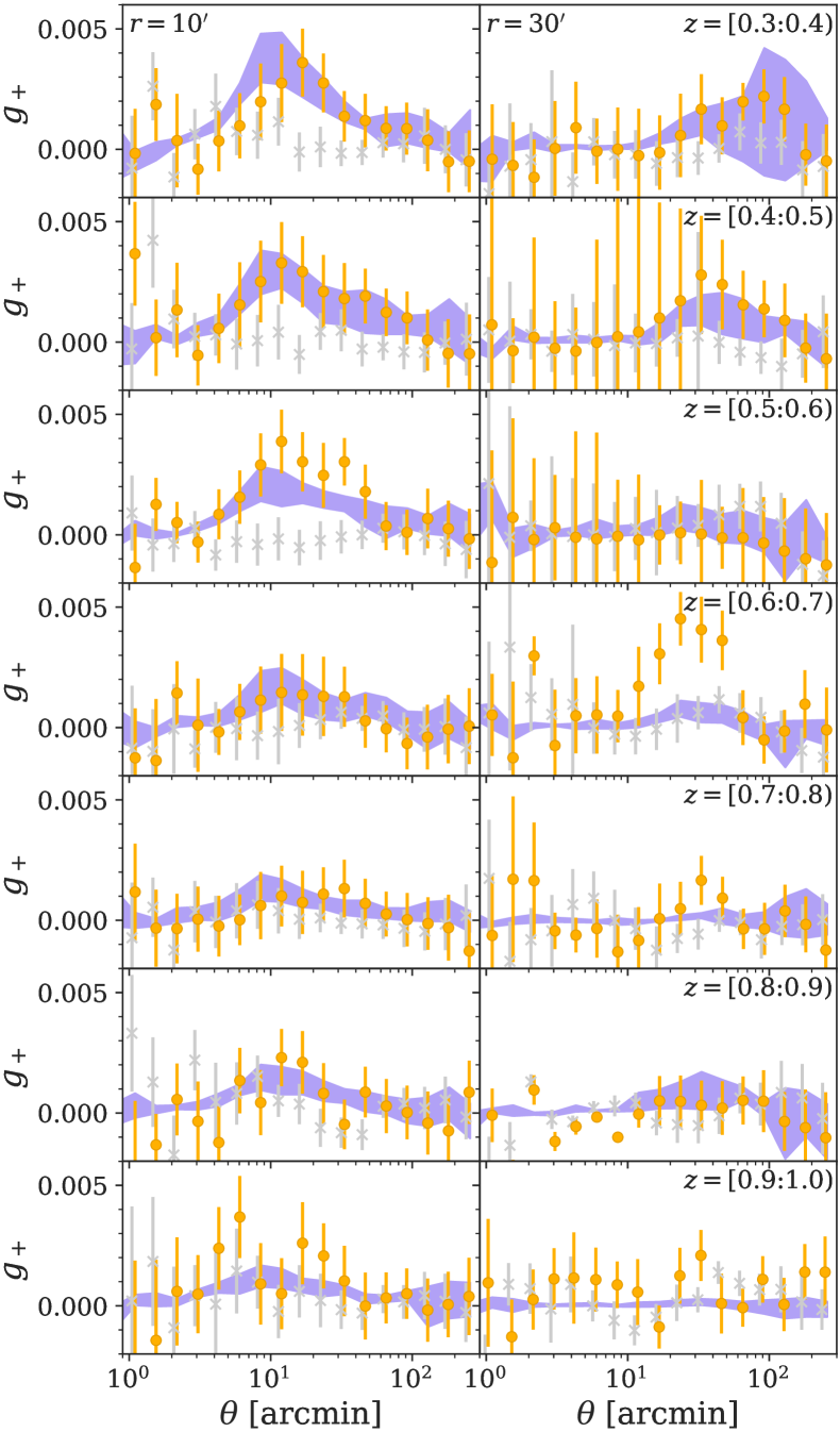
Figure 14: The orange circles and the grey cross symbols show the mean tangential and cross shear profiles from the weak lensing stacking for the over-densities with the number excess of $>3\sigma$ at $z=$ 0.3 – 1 in step of $\Delta z=0.1$ from top to bottom. Left and right panels respectively show the stacked lens signals for over-dense regions selected by $r=10$ and 30 arcmin apertures. The purple region indicates 68th percentiles of the mean tangential profiles from the mock shape catalogue based on 30 realisations.

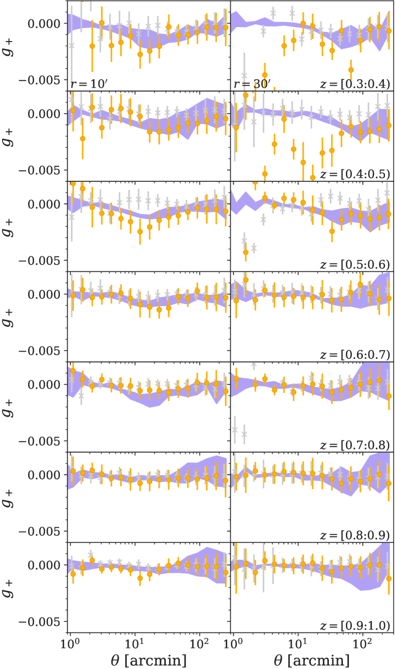
Figure 15: Same as Figure 14 but the mean tangential shear profiles for the under-dense regions with the number deficit of $<-1.5\sigma$.

5 Conclusion

Based on the HSC-SSP PDR2 data, we estimate projected number densities of $i$-band selected sources ($i<23$ mag) from $z=0.3$ to $z=1$ in step with $\Delta z=0.1$, within two different aperture areas ($r=10$ and 30 arcmin). This paper mainly focuses on the large-scale density contrasts based on the latter aperture size, though the former one would be more practical for the purpose of spectroscopic follow-up observations. The wide-field and deep HSC data successfully demonstrate the large-scale structure over 360 sq. degree fields, including the confirmation of known superclusters at $z=$ 0.8 – 1. By applying the same technique to the mock galaxy catalogue generated from the all-sky ray-tracing cosmological simulation, we find that the projected over-densities well trace the total masses of embedded massive dark matter haloes at each redshift slice. While the significant density peaks are expected to host one or more cluster-scale haloes at corresponding redshifts, the density troughs, top candidates of distant cosmic voids, would remarkably lack the matters and massive dark matter haloes. The significant density peaks and troughs at $z\lesssim 0.6$ are also confirmed with the mean lens shear signals from the weak lensing stacking analysis.

Thus far, intensive spectroscopic follow-up observations have been executed to a few superclusters at $z\sim 1$ (Gal et al., 2008; Lubin et al., 2009; Lietzen et al., 2016; Paulino-Afonso et al., 2018), though an extensive and comprehensive spectroscopic database has not yet been formed for mid and high redshift superclusters and voids. Thus a massive spectroscopic survey, like DESI (DESI Collaboration et al., 2016), PFS (Takada et al., 2014), MOONS (Cirasuolo et al., 2011) and 4MOST (de Jong et al., 2019) is imperative to address detailed structures of galaxies associated with the colossal over- and under-densities. Besides, eROSITA (Merloni et al., 2012), the Vera C. Rubin Observatory (Ivezić et al., 2019), Euclid (Amendola et al., 2018), and the Roman Space Telescope (Doré et al., 2019) are crucial to accumulate systematic information of such enormous structures or extend samples to the earlier universe.

Lastly, we should note that there remains substantial scope for improvement in our analyses, e.g., mask correction and removal of contaminants that are not perfect in PDR2 (Aihara et al., 2019). These caveats will be addressed with the third or later data release, as our data reduction pipeline keeps improving the data quality.

Data Availability

The data underlying this article are all available under the public data release site of Hyper Suprime-Cam Subaru Strategic Program (https://hsc.mtk.nao.ac.jp/ssp/data-release/).

Appendix A Density map catalogue

The projected density map catalogue at $z=$ 0.3 – 1 is available as grid-point data through the HSC-SSP website. We set an adequately small grid size of $\Delta=\sim 1.5\times 1.5$ square arcmin to the aperture size ($r=$ 10 or 30 arcmin) so that e.g., one can smooth and adjust the aperture size to the same comoving scale across the redshift bins if desired. Each pixel includes the number densities and the number excesses within each aperture at seven redshift slices: $z=$ [0.3:0.4), [0.4:0.5), [0.5:0.6), [0.6:0.7), [0.7:0.8), [0.8:0.9), and [0.9:1.0). The density information broken down to the narrower redshift range of $\Delta z=0.02$ is available as well. The accessible information is summarised in Table 1 where delta is the number excess in variance, $(n_{\mathrm{r}}-n_{\mathrm{r,mean}})/n_{\mathrm{r,mean}}$. $n_{\mathrm{r}}$ is a number density within a radius of 10 arcmin or 30 arcmin, and $n_{\mathrm{r,mean}}$ is the mean value of $n_{\mathrm{r}}$ at each redshift in the whole survey area. The columns #4 ix and #5 iy are grid id which correspond to the grid size in each survey field summarised in Table 1. They may be useful for reproducing the projected density map like Figure 6-8. The following script is an example to define a mesh grid of the W01 HectoMAP field for a Python visualisation tool: matplotlib (Hunter, 2007) with numpy package (Harris et al., 2020),

xmin, xmax = 224, 250
ymin, ymax = 42, 45
nx, ny = 754, 120
x0 = numpy.linspace(xmin, xmax, nx, endpoint=False)
y0 = numpy.linspace(ymin, ymax, ny, endpoint=False)
X, Y = numpy.meshgrid(x0, y0),

and then users can associate the grid points with density values in the target redshift range through ix and iy.

We should noted that, given the wide-field coverage, we have not conducted visual data inspections for individual regions. Thus, users must handle the catalogue with care at their own risk. For instance, when users make a plan of a spectroscopic follow-up observation towards their interesting fields based on the catalogue, we highly recommend to check the actual images taken from HSC around the targets as the minimum quality check through the user-friendly online visualisation tool called hscMAP. Users may also want to check the more detailed image quality such as the seeing size and the image depth. In such a case, refer #6 skymap_id to obtain the detailed information of the appropriate track and patch. The survey field of HSC-SSP is split to $\sim 1.7\times 1.7$ degree areas called tract, and further divided into $\sim 12\times 12$ arcmin field called patch (Aihara et al., 2019). Users can find such information for each track and patch stored in the HSC-SSP PDR2 database.

Table 2: Contents of the density map catalogue.

#	Name	Description
1	ra	R.A. [degree] of the centre of aperture
2	dec	Dec. [degree] of the centre of aperture
3	field	Field id (see Table 1)
4	ix	Pixel id in each field on the R.A. axis
5	iy	Pixel id in each field on the Dec. axis
6	skymap_id	Nearest tract and patch in HSC-SSP
7	eff_r10	Fraction of effective area in $r$=10 arcmin
8	eff_r30	Fraction of effective area in $r$=30 arcmin
9	nd3_r10	The number of $z$=[0.3:0.4) sources in $r$=10′
10	nd3_r30	The number of $z$=[0.3:0.4) sources in $r$=30′
11	sgm3_r10	Contrast of nc3_r10 in standard deviation
12	sgm3_r30	Contrast of nc3_r30 in standard deviation
13	dlt3_r10	Contrast of nc3_r10 in variance
14	dlt3_r30	Contrast of nc3_r30 in variance
15	n3_02_r10	The number of $z$=[0.30:0.32) sources in $r$=10′
16	n3_02_r30	The number of $z$=[0.30:0.32) sources in $r$=30′
17	n3_24_r10	The number of $z$=[0.32:0.34) sources in $r$=10′
18	n3_24_r30	The number of $z$=[0.32:0.34) sources in $r$=30′
19	n3_46_r10	The number of $z$=[0.34:0.36) sources in $r$=10′
20	n3_46_r30	The number of $z$=[0.34:0.36) sources in $r$=30′
21	n3_68_r10	The number of $z$=[0.36:0.38) sources in $r$=10′
22	n3_68_r30	The number of $z$=[0.36:0.38) sources in $r$=30′
23	n3_80_r10	The number of $z$=[0.38:0.40) sources in $r$=10′
24	n3_80_r30	The number of $z$=[0.38:0.40) sources in $r$=30′
25–40		Same as #9–24 but for $z$=[0.4:0.5)
41–46		Same as #9–24 but for $z$=[0.5:0.6)
47–62		Same as #9–24 but for $z$=[0.6:0.7)
63–78		Same as #9–24 but for $z$=[0.7:0.8)
79–94		Same as #9–24 but for $z$=[0.8:0.9)
95–110		Same as #9–24 but for $z$=[0.9:1.0)
111	eff_z3	Same as #7 but for $r$=10 cMpc at $z$=[0.3:0.4)
112	eff_z4	Same as #7 but for $r$=10 cMpc at $z$=[0.4:0.5)
113	eff_z5	Same as #7 but for $r$=10 cMpc at $z$=[0.5:0.6)
114	eff_z6	Same as #7 but for $r$=10 cMpc at $z$=[0.6:0.7)
115	eff_z7	Same as #7 but for $r$=10 cMpc at $z$=[0.7:0.8)
116	eff_z8	Same as #7 but for $r$=10 cMpc at $z$=[0.8:0.9)
117	eff_z9	Same as #7 but for $r$=10 cMpc at $z$=[0.9:1.0)
118	sgm3_c10	Same as #11 but for $r$=10 cMpc at $z$=[0.3:0.4)
119	dlt3_c10	Same as #13 but for $r$=10 cMpc at $z$=[0.3:0.4)
120	sgm4_c10	Same as #11 but for $r$=10 cMpc at $z$=[0.4:0.5)
121	dlt4_c10	Same as #13 but for $r$=10 cMpc at $z$=[0.4:0.5)
122	sgm5_c10	Same as #11 but for $r$=10 cMpc at $z$=[0.5:0.6)
123	dlt5_c10	Same as #13 but for $r$=10 cMpc at $z$=[0.5:0.6)
124	sgm6_c10	Same as #11 but for $r$=10 cMpc at $z$=[0.6:0.7)
125	dlt6_c10	Same as #13 but for $r$=10 cMpc at $z$=[0.6:0.7)
126	sgm7_c10	Same as #11 but for $r$=10 cMpc at $z$=[0.7:0.8)
127	dlt7_c10	Same as #13 but for $r$=10 cMpc at $z$=[0.7:0.8)
128	sgm8_c10	Same as #11 but for $r$=10 cMpc at $z$=[0.8:0.9)
129	dlt8_c10	Same as #13 but for $r$=10 cMpc at $z$=[0.8:0.9)
130	sgm9_c10	Same as #11 but for $r$=10 cMpc at $z$=[0.9:1.0)
131	dlt9_c10	Same as #13 but for $r$=10 cMpc at $z$=[0.9:1.0)

Appendix B Impact of redshift uncertainties

This paper discusses the mass contents of various environments traced by the projected density map based on the mock catalogue from the cosmological simulation. While we employ a sufficiently wide redshift bin of $\Delta z=0.1$ relative to typical photo-$z$ uncertainties ($\sigma=0.04$), ideally, we have to incorporate photo-$z$ errors and contamination effects from outliers into the analyses. We therefore carry out a quick test to see how photo-$z$ uncertainties makes an impact on our discussions in this paper by building photo-$z$ variations into redshifts of the mock samples.

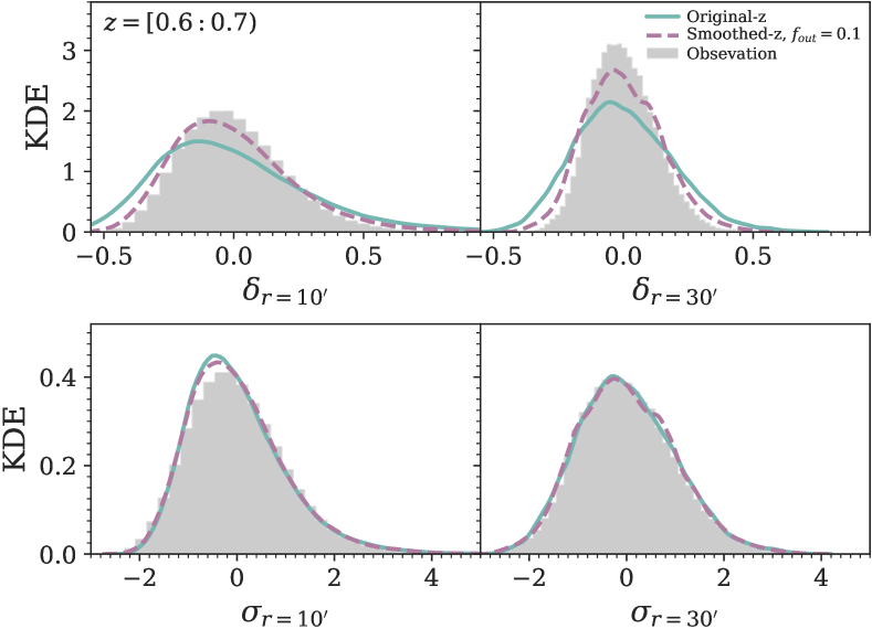
Figure 16: The upper and the lower panels respectively show variance and standard deviation of number densities within (left) $r=10$ arcmin and (right) $r=30$ arcmin apertures at $z=[0.6:0.7)$. The grey filled histogram is the normalised density distribution from the HSC-SSP PDR2 data (Fig. 4). The cyan curve (: original-$z$) and the purple dashed curves (: smoothed-$z$) indicate those KDE from the mock catalogue with and without the redshift variations, respectively (see text about the methodology).

In order to test the impacts of photo-$z$ errors on our analyses, we choose the intermediate redshift bin $z=[0.6:0.7)$ out of seven redshift slices in $z=0.3$ – 1 that we used in this paper, which allows us to add irrelevant sources from distant foreground ($z=0.3$ – 0.5) and background ($z=0.8$ – 1) redshifts into the sample. Firstly, we convolve redshifts of all mock sources at $z=0.3$ – 1 with a Gaussian filter with $\sigma=0.04$ according to the typical redshift dispersion of photometric redshifts from Mizuki for $i$-band ($i<23$) selected sources at $z<1$ (Tanaka et al., 2018). After that, we measure the number densities within $r=10$ or $r=30$ arcmin apertures at $z=[0.6:0.7)$ in the same way as for the HSC sample and the mock data (§3.2 and §4.1). In this process, we mix the randomly selected outliers in the foreground ($z=0.3$ – 0.5) or the background ($z=0.8$ – 1) in with the sample at $z=[0.6:0.7)$. The number of outliers are arranged to 10 per cent the outlier rate, $f_{out}\equiv N_{\mathrm{outlier}}/N_{\mathrm{total}}=0.1$, which is consistent with that of our sample (Tanaka et al., 2018). It should be noted that our simplified test would not produce an exact photo-$z$ error although this tells how irrelevant sources affect the density estimation: photometric redshift errors of galaxies are not random distribution, rather, the errors should be biased to certain redshift ranges depending on those SEDs and redshifts.

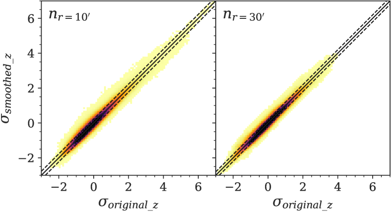
Figure 17: The number densities within $r=10$ arcmin (on the left) and $r=30$ arcmin (on the right) apertures in the standard deviation inclusive photo-$z$ uncertainties($\sigma_{\mathrm{originalz}}$), with respect to those inferred from the original mock sample ($\sigma_{\mathrm{smoothedz}}$). The solid and dashed diagonal lines indicate a one-to-one relation and $\pm 1\sigma$ deviations of the density contrast between with and without installing photo-$z$ errors.

The resultant density distribution in the variance and the standard deviation are presented in Figure 16. Those in consideration of photometric redshift errors show a broad agreement with the density distributions of the observed data, suggesting that the assumption of the large-scale galaxy bias (Nicola et al., 2020, eq. 4.11 and 4.12) in producing $i$-band selected mock sources works for our sample. Residual margin seen in the variances between the observation and the mock data (Fig. 16) can be minimised by assuming the outlier rate of $\sim 0.2$, which suggests that our sample may contain more contaminant foreground and/or background sources. Photo-$z$ uncertainties scatter the density contrast of original spatial distributions, as shown in Figure 17 and make the density variance spikier. Figure 16 and 17 also argue that original mock density distribution out of consideration of photo-$z$ errors can be used to test systematic trends as long as we employ the standard deviation as a tracer of the density contrast. Such a consensus of the density contrasts between with and without photo-$z$ uncertainties can also be recognised in the mock projected density maps shown in Figure 18. As a result, photometric redshift errors have a little influence on the discussion, as seen in Figure 19.

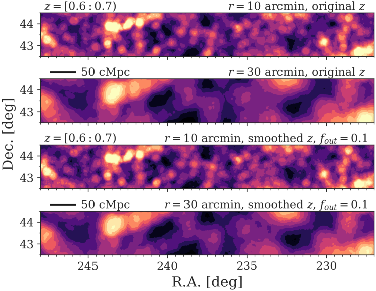
Figure 18: Example cutouts from the mock density maps at $z=[0.6:0.7)$ in W01 HectoMAP. From top to bottom, the density maps within $r=10$ and 30 arcmin apertures based on the original mock catalogue, and those within $r=10$ and 30 arcmin apertures from the mock sample that incorporates photo-$z$ uncertainties.

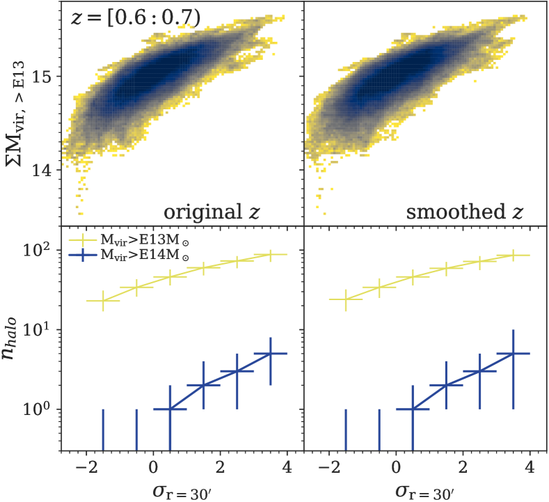
Figure 19: Same as Figure 13, but for the density distributions at $z=[0.6:0.7)$ without and with consideration of photo-$z$ uncertainties on the left and right sides, respectively.

Appendix C Online materials

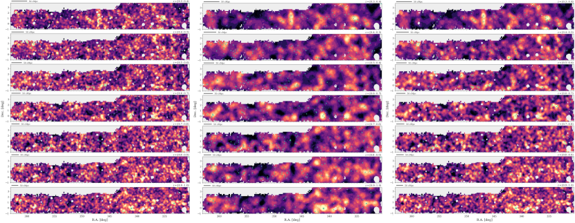
Figure 20: Same as Fig. 6– 8 but for W05 (VVDS).

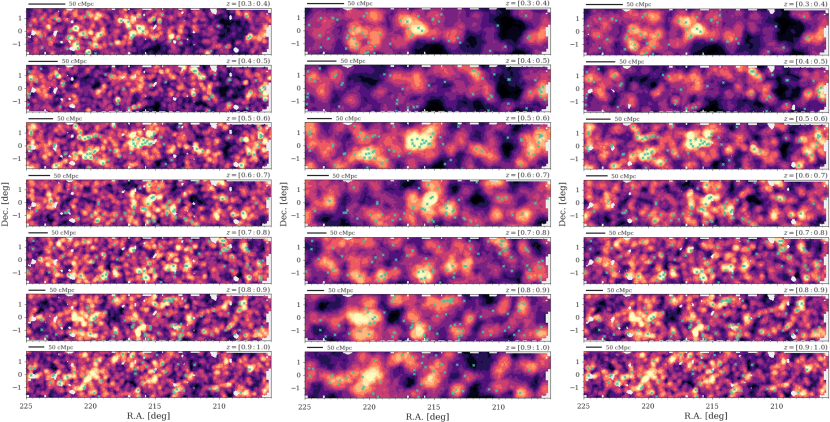
Figure 21: Same as Fig. 6– 8 but for W04 (GAMA15H).

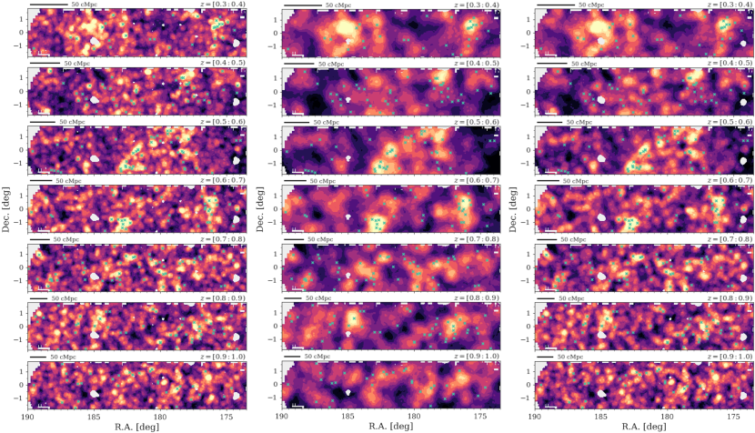
Figure 22: Same as Fig. 6– 8 but for W04 (WIDE12H).

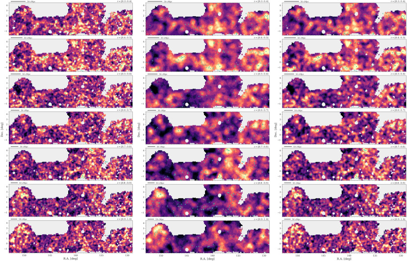
Figure 23: Same as Fig. 6– 8 but for W03 (GAMA09H).

References

- Abbott et al. (2018) Abbott T. M. C., et al., 2018, ApJS, 239, 18
- Agarwal & Feldman (2011) Agarwal S., Feldman H. A., 2011, MNRAS, 410, 1647
- Aihara et al. (2018a) Aihara H., et al., 2018a, PASJ, 70
- Aihara et al. (2018b) Aihara H., et al., 2018b, PASJ, 70, 1
- Aihara et al. (2019) Aihara H., et al., 2019, PASJ, 71, 2
- Alpaslan et al. (2015) Alpaslan M., et al., 2015, MNRAS, 451, 3249
- Amendola et al. (1999) Amendola L., Frieman J. A., Waga I., 1999, MNRAS, 309, 465
- Amendola et al. (2018) Amendola L., et al., 2018, Living Rev. Relativ., 21, 2
- Baldry et al. (2006) Baldry I. K., Balogh M. L., Bower R. G., Glazebrook K., Nichol R. C., Bamford S. P., Budavari T., 2006, MNRAS, 373, 469
- Bartelmann & Schneider (2001) Bartelmann M., Schneider P., 2001, Phys. Rep., 340, 291
- Behroozi et al. (2013) Behroozi P. S., Wechsler R. H., Wu H.-Y., 2013, ApJ, 762, 109
- Blanton et al. (2017) Blanton M. R., et al., 2017, AJ, 154, 28
- Bosch et al. (2018) Bosch J., et al., 2018, PASJ, 70, 1
- Cai et al. (2015) Cai Y.-C., Padilla N., Li B., 2015, MNRAS, 451, 1036
- Cirasuolo et al. (2011) Cirasuolo M., Afonso J., Bender R., Bonifacio P., Evans C., Kaper L., Oliva E., Vanzi L., 2011, The Messenger, 145, 11
- Clampitt et al. (2013) Clampitt J., Cai Y.-C., Li B., 2013, MNRAS, 431, 749
- Colless et al. (2001) Colless M., et al., 2001, MNRAS, 328, 1039
- Contarini et al. (2019) Contarini S., Ronconi T., Marulli F., Moscardini L., Veropalumbo A., Baldi M., 2019, MNRAS, 488, 3526
- Coupon et al. (2018) Coupon J., Czakon N., Bosch J., Komiyama Y., Medezinski E., Miyazaki S., Oguri M., 2018, PASJ, 70, 1
- DESI Collaboration et al. (2016) DESI Collaboration et al., 2016, arXiv e-prints, arXiv:1611.00036
- Davies et al. (2020) Davies C. T., Paillas E., Cautun M., Li B., 2020, arXiv e-prints, arXiv:2004.11387
- Dekel & Rees (1994) Dekel A., Rees M. J., 1994, ApJ, 422, L1
- Doré et al. (2019) Doré O., et al., 2019, arXiv e-prints, arXiv:1904.01174
- Douglass & Vogeley (2017) Douglass K. A., Vogeley M. S., 2017, ApJ, 834, 186
- Driver et al. (2009) Driver S. P., et al., 2009, Astron. Geophys., 50, 5.12
- Driver et al. (2011) Driver S. P., et al., 2011, MNRAS, 413, 971
- Eisenstein et al. (2011) Eisenstein D. J., et al., 2011, AJ, 142, 72
- Finelli et al. (2016) Finelli F., García-Bellido J., Kovács A., Paci F., Szapudi I., 2016, MNRAS, 455, 1246
- Furusawa et al. (2018) Furusawa H., et al., 2018, PASJ, 70, 1
- Gal et al. (2008) Gal R. R., Lemaux B. C., Lubin L. M., Kocevski D., Squires G. K., 2008, ApJ, 684, 933
- Geller & Hwang (2015) Geller M. J., Hwang H. S., 2015, Astron. Nachrichten, 336, 428
- Geller et al. (2011) Geller M. J., Diaferio A., Kurtz M. J., 2011, AJ, 142, 133
- Gorski et al. (2005) Gorski K. M., Hivon E., Banday A. J., Wandelt B. D., Hansen F. K., Reinecke M., Bartelmann M., 2005, ApJ, 622, 759
- Gregory & Thompson (1978) Gregory S. A., Thompson L. A., 1978, ApJ, 222, 784
- Gruen et al. (2016) Gruen D., et al., 2016, MNRAS, 455, 3367
- Gruen et al. (2018) Gruen D., et al., 2018, Phys. Rev. D, 98, 023507
- Gunn et al. (1986) Gunn J. E., Hoessel J. G., Oke J. B., 1986, ApJ, 306, 30
- Hamana & Mellier (2001) Hamana T., Mellier Y., 2001, MNRAS, 327, 169
- Harris et al. (2020) Harris C. R., et al., 2020, Nature, 585, 357
- Hayashi et al. (2019) Hayashi M., et al., 2019, PASJ, 71, 1
- Heymans et al. (2012) Heymans C., et al., 2012, MNRAS, 427, 146
- Heymans et al. (2013) Heymans C., et al., 2013, MNRAS, 432, 2433
- Higuchi & Inoue (2018) Higuchi Y., Inoue K. T., 2018, MNRAS, 476, 359
- Higuchi & Inoue (2019) Higuchi Y., Inoue K. T., 2019, MNRAS, 488, 5811
- Higuchi & Shirasaki (2016) Higuchi Y., Shirasaki M., 2016, MNRAS, 459, 2762
- Higuchi et al. (2013) Higuchi Y., Oguri M., Hamana T., 2013, MNRAS, 432, 1021
- Hikage et al. (2019) Hikage C., et al., 2019, PASJ, 71, 1
- Hildebrandt et al. (2017) Hildebrandt H., et al., 2017, MNRAS, 465, 1454
- Hinshaw et al. (2013) Hinshaw G., et al., 2013, ApJS, 208, 19
- Hunter (2007) Hunter J. D., 2007, Comput. Sci. Eng., 9, 90
- Inoue & Silk (2006) Inoue K. T., Silk J., 2006, ApJ, 648, 23
- Inoue & Silk (2007) Inoue K. T., Silk J., 2007, ApJ, 664, 650
- Ivezić et al. (2019) Ivezić Ž., et al., 2019, ApJ, 873, 111
- Kawanomoto et al. (2018) Kawanomoto S., et al., 2018, PASJ, 70, 1
- Kirshner et al. (1981) Kirshner R. P., Oemler, A. J., Schechter P. L., Shectman S. A., 1981, ApJ, 248, L57
- Komiyama et al. (2018) Komiyama Y., et al., 2018, PASJ, 70, 1
- Lemaux et al. (2017) Lemaux B. C., Tomczak A. R., Lubin L. M., Wu P.-F., Gal R. R., Rumbaugh N., Kocevski D. D., Squires G. K., 2017, MNRAS, 472, 419
- Lewis et al. (2000) Lewis A., Challinor A., Lasenby A., 2000, ApJ, 538, 473
- Lietzen et al. (2016) Lietzen H., et al., 2016, A&A, 588, L4
- Lin et al. (2017) Lin Y.-T., et al., 2017, ApJ, 851, 139
- Liske et al. (2015) Liske J., et al., 2015, MNRAS, 452, 2087
- Lubin et al. (2000) Lubin L. M., Brunner R., Metzger M. R., Postman M., Oke J. B., 2000, ApJ, 531, L5
- Lubin et al. (2009) Lubin L. M., Gal R. R., Lemaux B. C., Kocevski D. D., Squires G. K., 2009, AJ, 137, 4867
- Mandelbaum et al. (2006) Mandelbaum R., Seljak U., Cool R. J., Blanton M., Hirata C. M., Brinkmann J., 2006, MNRAS, 372, 758
- Mandelbaum et al. (2018) Mandelbaum R., et al., 2018, PASJ, 70, 2
- McKinney (2010) McKinney W., 2010, Proc. 9th Python Sci. Conf., 1697900, 51
- Merloni et al. (2012) Merloni A., et al., 2012, arXiv e-prints, arXiv:1209.3114
- Miyazaki et al. (2018) Miyazaki S., et al., 2018, PASJ, 70
- Moutard et al. (2020) Moutard T., Sawicki M., Arnouts S., Golob A., Coupon J., Ilbert O., Yang X., Gwyn S., 2020, MNRAS, 494, 1894
- Nicola et al. (2020) Nicola A., et al., 2020, J. Cosmol. Astropart. Phys., 2020, 044
- Nishizawa et al. (2018) Nishizawa A. J., et al., 2018, PASJ, 70, 1
- Oguri (2014) Oguri M., 2014, MNRAS, 444, 147
- Oguri et al. (2012) Oguri M., Bayliss M. B., Dahle H., Sharon K., Gladders M. D., Natarajan P., Hennawi J. F., Koester B. P., 2012, MNRAS, 420, 3213
- Oguri et al. (2018) Oguri M., et al., 2018, PASJ, 70, 1
- Okabe et al. (2010) Okabe N., Takada M., Umetsu K., Futamase T., Smith G. P., 2010, PASJ, 62, 811
- Oke & Gunn (1983) Oke J. B., Gunn J. E., 1983, ApJ, 266, 713
- Oort (1983) Oort J. H., 1983, ARA&A, 21, 373
- Park et al. (2007) Park C., Choi Y., Vogeley M. S., Gott III J. R., Blanton M. R., 2007, ApJ, 658, 898
- Paulino-Afonso et al. (2018) Paulino-Afonso A., Sobral D., Darvish B., Ribeiro B., Stroe A., Best P., Afonso J., Matsuda Y., 2018, A&A, 620, A186
- Peebles (2001) Peebles P. J. E., 2001, ApJ, 557, 495
- Peng et al. (2010) Peng Y.-j., et al., 2010, ApJ, 721, 193
- Pisani et al. (2015) Pisani A., Sutter P. M., Hamaus N., Alizadeh E., Biswas R., Wandelt B. D., Hirata C. M., 2015, Phys. Rev. D, 92
- Regos & Geller (1991) Regos E., Geller M. J., 1991, ApJ, 377, 14
- Robitaille et al. (2013) Robitaille T. P., et al., 2013, A&A, 558, A33
- Rojas et al. (2005) Rojas R. R., Vogeley M. S., Hoyle F., Brinkmann J., 2005, ApJ, 624, 571
- Sawicki et al. (2019) Sawicki M., et al., 2019, MNRAS, 489, 5202
- Scoville et al. (2007) Scoville N., et al., 2007, ApJS, 172, 1
- Shirasaki et al. (2015) Shirasaki M., Hamana T., Yoshida N., 2015, MNRAS, 453, 3044
- Shirasaki et al. (2017) Shirasaki M., Takada M., Miyatake H., Takahashi R., Hamana T., Nishimichi T., Murata R., 2017, MNRAS, 470, 3476
- Shirasaki et al. (2019) Shirasaki M., Hamana T., Takada M., Takahashi R., Miyatake H., 2019, MNRAS, 486, 52
- Sorrentino et al. (2006) Sorrentino G., Antonuccio-Delogu V., Rifatto A., 2006, A&A, 460, 673
- Sousbie (2011) Sousbie T., 2011, MNRAS, 414, 350
- Springel (2005) Springel V., 2005, MNRAS, 364, 1105
- Steinhardt et al. (2014) Steinhardt C. L., et al., 2014, ApJ, 791, L25
- Szapudi et al. (2015) Szapudi I., et al., 2015, MNRAS, 450, 288
- Tadaki et al. (2020) Tadaki K.-i., Iye M., Fukumoto H., Hayashi M., Rusu C. E., Shimakawa R., Tosaki T., 2020, arXiv e-prints, arXiv:2006.13544
- Takada et al. (2014) Takada M., et al., 2014, PASJ, 66, R1
- Takahashi et al. (2017) Takahashi R., Hamana T., Shirasaki M., Namikawa T., Nishimichi T., Osato K., Shiroyama K., 2017, ApJ, 850, 24
- Tanaka (2015) Tanaka M., 2015, ApJ, 801, 20
- Tanaka et al. (2004) Tanaka M., Goto T., Okamura S., Shimasaku K., Brinkmann J., 2004, AJ, 128, 2677
- Tanaka et al. (2018) Tanaka M., et al., 2018, PASJ, 70, 1
- Taylor (2005) Taylor M. B., 2005, Astron. Data Anal. Softw. Syst. XIV - ASP Conf. Ser., 347, 29
- Toshikawa et al. (2018) Toshikawa J., et al., 2018, PASJ, 70, 1
- York et al. (2000) York D. G., et al., 2000, AJ, 120, 1579
- de Jong et al. (2013) de Jong J. T. A., Verdoes Kleijn G. A., Kuijken K. H., Valentijn E. A., 2013, Exp. Astron., 35, 25
- de Jong et al. (2019) de Jong R. S., et al., 2019, The Messenger, 175, 3
- de Vaucouleurs (1953) de Vaucouleurs G., 1953, AJ, 58, 30