Connection matrices in combinatorial topological dynamics

Abstract.

Connection matrices are one of the central tools in Conley’s approach to the study of dynamical systems, as they provide information on the existence of connecting orbits in Morse decompositions. They may be considered as a generalization of the Morse complex boundary operator in Morse theory. Their computability has recently been addressed by Harker, Mischaikow, and Spendlove [14] in the context of lattice filtered chain complexes. In the current paper, we extend the newly introduced Conley theory for combinatorial vector and multivector fields on Lefschetz complexes [24] by transferring the concept of connection matrix to this setting. This is accomplished by connection matrices for arbitrary poset filtered chain complexes, as well as an associated equivalence, which allows for changes in the underlying posets. We show that for the special case of gradient combinatorial vector fields in the sense of Forman [12], connection matrices are necessarily unique. Thus, the classical results of Reineck [33, 34] have a natural analogue in the combinatorial setting.

1. Introduction

Classical Morse theory concerns a compact smooth manifold together with a smooth real-valued function with non-degenerate critical points. An important part of the theory introduces the Morse complex which is a chain complex whose $i$th chain group is a free abelian group spanned by critical points of Morse index $i$ and whose boundary homomorphism is defined by counting the (oriented) flow lines between critical points in the gradient flow induced by the Morse function (see [20, Section 4.2]). One of the fundamental results of classical Morse theory states that the homology of the manifold is isomorphic to the homology of the Morse complex.

The stationary points of the gradient flow in Morse theory, which are precisely the critical points of the Morse function, provide the simplest example of an isolated invariant set, a key concept of Conley theory [6]. For every isolated invariant set there is a homology module associated with it. It is called the homology Conley index. A (minimal) Morse decomposition is a decomposition of space into a partially ordered collection of isolated invariant sets, called Morse sets, such that every recurrent trajectory (in particular every stationary or periodic trajectory) is located in a Morse set and every non-recurrent trajectory is a heteroclinic connection between Morse sets from a higher Morse set to a lower Morse set in the poset structure of the Morse decomposition. The collection of stationary points of the gradient flow of a Morse function provides the simplest example of a Morse decomposition in which the Morse sets are just the stationary points and the Conley index of a stationary point coincides with the homology of a pointed $k$-dimensional sphere with $k$ equal to the Morse index of the point.

Conley theory in its simplest form may be viewed as a twofold generalization of Morse theory. On the one hand, it substantially weakens the general assumptions by replacing the smooth manifold by a compact metric space and the gradient flow of the Morse function by an arbitrary (semi)flow. On the other hand, it replaces the collection of critical points of the Morse function by the more general Morse decomposition in which the counterpart of the Morse complex takes the form of the direct sum of the Conley indexes of all Morse sets. The homology of this generalized complex, as in the Morse theory, is isomorphic to the homology of the space. The boundary operator in this setting is called the connection matrix of the Morse decomposition. This definition of connection matrix was introduced by Franzosa in [13]. His definition, based on homology braids, is technically complicated, in part because the generalized setting captures the situations of bifurcations when, unlike for Morse theory, the connection matrix need not be uniquely determined by the flow. In a later paper Robbin and Salamon [35] simplify slightly the definition by replacing homology braids with filtered chain complexes which helps with separating dynamics from algebra. This separation is even more visible in the recent algorithmic approach to connection matrices by Harker, Mischaikow, and Spendlove [14]. Actually, the separation of dynamics and algebra allows the authors in [14, 35] to set up the definition of a connection matrix of a Morse decomposition along the following pipeline, where we omit a number of technical details:

• Consider a Morse decomposition $\text{$\mathcal{M}$}:=\{M_{p}\}_{p\in P}$ of the phase space indexed by a poset $P$.

• For each down set $I\subset P$ consider the associated attractor $M_{I}$ consisting of points on trajectories whose limits sets are in $\bigcup_{p\in I}M_{p}$ and construct an attracting neighborhood $N_{I}$ for the attractor $M_{I}$ in such a way that $I\mapsto N_{I}$ is a lattice homomorphism.

• Under some smoothness assumptions the family $\{N_{I}\}$ of step (ii) induces a $P$-filtered chain complex.

• A connection matrix of $\mathcal{M}$ is an algebraic object associated with a poset filtered chain complex, in particular with the $P$-filtered chain complex of step (iii).

Conley theory, in particular via connection matrices, is a very useful tool in the qualitative study of dynamical systems. However, to apply it one requires a well-defined dynamical system on a compact metric space. This is not the case when the dynamical system is exposed only via a finite set of samples as in the case of time series collected from observations or experiments. The study of dynamical systems known only from samples becomes an important part of the rapidly growing field of data science. In this context a generalization of Morse theory presented by Robin Forman [12] turns out to be very fruitful. In this generalization the smooth manifold is replaced by a finite CW complex and the gradient vector field of the Morse function by the concept of a combinatorial vector field. These structures may be easily constructed from data and analyzed by means of the combinatorial, also called discrete, Morse theory by Forman.

Recently, the concepts of isolated invariant set and Conley index have been carried over to this combinatorial setting [4, 18, 24, 27, 30]. In the present paper we extend these ideas by constructing connection matrices of a Morse decomposition of a combinatorial multivector field. To achieve this, we have to modify the connection matrix pipeline discussed above, because in the combinatorial case, and even in the case of a multiflow, step (ii) in the pipeline cannot be completed in general. To overcome this difficulty we enlarge the original poset to guarantee the existence of the necessary lattice of attracting neighborhoods. The added elements are then removed by introducing a certain equivalence in the category of poset filtered chain complexes with a varying poset structure. A side benefit of this approach is the shortening of the pipeline by omitting step (ii). Such a shortening is possible, because, under the enlarged poset, the filtered chain complex of step (iii) may be obtained directly from the Morse decomposition via an associated partition of the phase space indexed by the extended poset. The proposed theory of connection matrices for combinatorial multivector fields lets us prove the main result of the paper: The uniqueness of connection matrices for gradient combinatorial Forman vector fields.

Although the main motivation for our paper is the adaptation of connection matrix theory to the combinatorial setting of multivector fields, we believe that the approach presented here has broader potential. Formally speaking, connection matrices are purely algebraic objects and are presented this way from the very beginning. Nevertheless, in the early papers they are strongly tied to dynamical considerations. In particular, the important concept of uniqueness and non-uniqueness in these papers is addressed only via the underlying dynamics. As we already mentioned, the decoupling of algebra and dynamics started with Robbin and Salamon [35], and is even stronger in Harker, Mischaikow, and Spendlove [14]. However, to the best of our knowledge, so far there has been no purely algebraic definition of uniqueness. Harker, Mischaikow, and Spendlove [14] prove that any two connection matrices of the same filtered chain complex are conjugate via a filtered isomorphism. Clearly, this is not the uniqueness concept used in the context of dynamics. In our approach we propose a stronger algebraic equivalence of connection matrices which allows for filtered chain complexes with no unique connection matrix. We use this definition in the already mentioned main result of our paper on the uniqueness of connection matrices for gradient combinatorial vector fields. We believe that the detachment of connection matrix theory from dynamics is worth the effort, because it may bring applications in new fields. The potential of applications in topological data analysis is already discussed in [14], and the ties between connection matrices and persistent homology are also visible in [8]. Moreover, combinatorial vector fields have been used successfully in the study of algebraic and combinatorial problems [15, 21, 36].

Finally, combinatorial multivector fields make it possible to construct examples of a variety of complex dynamical phenomena in a straightforward way. It is therefore our hope that the results of this paper make topological methods in dynamics, and in particular the concept of connection matrices, more accessible to a broader mathematical audience.

The remainder of this paper is organized as follows. In Section 2 we provide an informal overview over our main definitions and results. By providing numerous examples, we hope that this section will serve as a guide for the more technical later sections of the paper. In addition, this section can serve as a quick and informal introduction to the concept of connection matrices. After presenting necessary preliminary definitions and facts in Section 3, the main technical part of the paper starts with a discussion of poset graded and poset filtered chain complexes in Section 4. Based on these definitions, the algebraic connection matrix can then be introduced in Section 5. The remaining three sections of the paper apply the earlier algebraic constructions to multivector fields on Lefschetz complexes. While the connection matrix in this setting is considered in Section 6, the dynamics of combinatorial multivector fields is the subject of Section 7. Finally, in Section 8 we show that if one considers a gradient Forman vector field on a Lefschetz complex, then the associated connection matrix is necessarily uniquely determined.

2. Main results

In this section we informally summarize our definition of connection matrices in the combinatorial setting, together with the necessary background material, examples, and main results of the paper. Precise definitions, statements, and proofs will be given in the sequel. We emphasize that throughout the paper we assume field coefficients in all considered modules, in particular in chain complexes and homology modules.

2.1. Combinatorial dynamical systems and multivector fields

By a combinatorial dynamical system we mean a multivalued map $F:X\multimap X$ defined on a finite topological space $X$. Alternatively, it may be viewed as a finite directed graph whose set of vertices is the topological space $X$, and with $F$ interpreted as the map sending a vertex to the collection of its neighbors connected via an outgoing directed edge. We call it the $F$-digraph. In most applications, this set $X$ of vertices of the $F$-digraph is a collection or certain subcollection of cells of a finite cellular complex, for instance a simplicial complex, with its topology induced by the associated face poset via the Alexandrov Theorem [1]. This topology is very different from the metric topology of the geometric realization of the cellular complex in terms of its separation properties, but the same in terms of homotopy and homology groups via McCord’s Theorem [26]. Hence, as far as algebraic topological invariants are concerned, these topologies may be used interchangeably, with the finite topology having the advantage of better explaining some peculiarities of combinatorial dynamics.

As in classical multivalued dynamics, given a combinatorial dynamical system $F$, we define a solution of $F$ to be a map $\gamma:I\to X$ defined on a subset $I\subset\mbox{$\mathbb{Z}$}$ of integers and such that $\gamma(i+1)\in F(\gamma(i))$ for $i,i+1\in I$. The solution $\gamma$ is called full if $I=\mbox{$\mathbb{Z}$}$, and it is a path if $I$ is the intersection of $\mathbb{Z}$ with a compact interval in $\mathbb{R}$. In the directed graph interpretation, a solution may be viewed as a finite or infinite directed walk through the graph. Finally, a subset $A\subset X$ is called invariant if for every point $a\in A$ there exists a full solution $\gamma:\mbox{$\mathbb{Z}$}\to A$ through the point $a$, that is, a solution satisfying the identity $\gamma(0)=a$.

In this paper we are interested in a class of combinatorial dynamical systems induced by combinatorial vector and multivector fields. We recall that a combinatorial multivector field $\mathcal{V}$ is a partition of a finite topological space $X$ into multivectors, where a multivector is a locally closed set, that is, a set which is the difference of two closed sets (see [10]). A multivector is called a vector, if its cardinality is one or two. If a combinatorial multivector field contains only vectors, then we call it a combinatorial vector field, a concept introduced already by Forman [12]. In applications, the partition indicates the resolution below which there is not enough evidence to analyse the dynamics either due to insufficient amount of data or because of lacking computational power.

The results of this paper require the combinatorial multivector field to be defined on a special finite topological space, namely a Lefschetz complex [23], called by Lefschetz and in [14] simply a complex. In short, a Lefschetz complex is just a basis $X$ of a finitely generated free chain complex $(C,d)$ with emphasis on the basis. This means that $X$ is the Lefschetz complex and $(C,d)$, denoted $C(X)$, is the chain complex associated with the Lefschetz complex. In terms of applications, a typical example of a Lefschetz complex is the set of cells of a cellular complex or simplices of a simplicial complex. These simplices or cells constitute a natural basis for the associated chain complex. Also, every locally closed subset of a Lefschetz complex is a Lefschetz complex, a feature which, in particular, facilitates constructing concise examples. By the homology of a Lefschetz complex $X$ we mean the homology of the associated chain complex $C(X)$. We view a Lefschetz complex as a finite topological space via the Alexandrov Theorem. For this, we need a well-defined face relation, which is given by the transitive closure of the facet relation, where an element $x\in X$ is called a facet of $y\in X$ if $x$ appears with non-zero coefficient in the boundary $d(y)$.

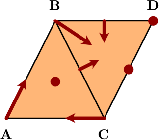
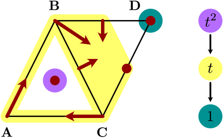
Figure 1. A first multivector field. The left panel shows a combinatorial multivector field on a simplicial complex which consists of two triangles, five edges, and four vertices. The multivector field has three critical cells, marked as red dots, two vectors on the bottom and left-most edges, as well as one multivector, which consists of the right triangle $\mathbf{B}\mathbf{C}\mathbf{D}$, its two edges $\mathbf{B}\mathbf{C}$ and $\mathbf{B}\mathbf{D}$, and the vertex $\mathbf{B}$. In the middle panel, we indicate the three Morse sets of the associated combinatorial dynamical system $F_{\text{$\mathcal{V}$}}$ in purple, yellow, and green, while the Conley-Morse graph of this Morse decomposition is shown in the panel on the right.

Example 2.1 (A first multivector field).

Figure 1(left) presents an example of a combinatorial multivector field on a Lefschetz complex $X$ which is just a simplicial complex consisting of two triangles $\mathbf{A}\mathbf{B}\mathbf{C}$, $\mathbf{B}\mathbf{C}\mathbf{D}$, five edges $\mathbf{A}\mathbf{B}$, $\mathbf{A}\mathbf{C}$, $\mathbf{B}\mathbf{C}$, $\mathbf{B}\mathbf{D}$, $\mathbf{C}\mathbf{D}$, and four vertices $\mathbf{A}$, $\mathbf{B}$, $\mathbf{C}$, $\mathbf{D}$. Hence, $X$ is a finite topological space consisting of eleven elements. The combinatorial multivector field in Figure 1 consists of three singletons $\{\mathbf{A}\mathbf{B}\mathbf{C}\}$, $\{\mathbf{C}\mathbf{D}\}$, and $\{\mathbf{D}\}$ indicated in the figure by a red dot, two doubletons $\{\mathbf{A},\mathbf{A}\mathbf{B}\}$ and $\{\mathbf{C},\mathbf{A}\mathbf{C}\}$ marked with a red arrow, and one multivector $\{\mathbf{B},\mathbf{B}\mathbf{C},\mathbf{B}\mathbf{D},\mathbf{B}\mathbf{C}\mathbf{D}\}$ consisting of four simplices and marked with red arrows joining each simplex in the multivector with its top-dimensional coface in the same multivector. Why this method of drawing multivectors is natural will become clear when we discuss the combinatorial dynamical system induced by the combinatorial multivector field. $\Diamond$

Every combinatorial multivector field $\mathcal{V}$ induces a combinatorial dynamical system $F_{\text{$\mathcal{V}$}}:X\multimap X$ given for $x\in X$ by

(1) $$F_{\text{$\mathcal{V}$}}(x):=\operatorname{cl}x\cup[x]_{\text{$\mathcal{V}$}}\;.$$

In this definition, $\operatorname{cl}x$ stands for the closure of $x$ in $X$, that is, it is given by the collection of all faces of $x$. Moreover, $[x]_{\text{$\mathcal{V}$}}$ denotes the unique multivector $V$ in the partition $\mathcal{V}$ with $x\in V$. The formula for $F_{\text{$\mathcal{V}$}}$ is related to the resolution interpretation of a combinatorial multivector field mentioned earlier. Namely, inside a multivector we do not exclude any movement, treating a multivector as kind of a black box. This justifies the presence of $[x]_{\text{$\mathcal{V}$}}$ in (1). And, since the dynamics of a combinatorial multivector field models a flow, any movement between multivectors is possible only through their common boundary. This justifies the presence of the closure $\operatorname{cl}x$ in (1).

Example 2.2 (A first multivector field, continued).

Even for a simple multivector field such as the one shown in Figure 1(left) the induced combinatorial dynamical system is quite large. Interpreted as a directed graph, it has eleven vertices (one for each simplex) and $42$ directed edges. Hence, instead of drawing such a digraph, we interpret Figure 1(left) as a digraph with vertices in the centers of mass of simplices (not marked) and only a minimum of directed edges (arrows) which cannot be deduced from (1). In fact, the only arrows which do depend on $\mathcal{V}$ are arrows of the form $x\to y$ where $y\in[x]_{\text{$\mathcal{V}$}}\setminus\operatorname{cl}x$. Moreover, since vertices inside the same multivector form a clique in the directed graph, it suffices to mark only some of the arrows joining them and, as we already mentioned, we mark arrows joining each simplex in the multivector with its top-dimensional cofaces in the same multivector. Interpreting Figure 1(left) this way, it is not difficult to infer the solutions of $F_{\text{$\mathcal{V}$}}$ from the figure. For instance, we have a solution $\gamma$ defined for $n\in\mbox{$\mathbb{Z}$}$ by

$$\gamma(n):=\begin{cases}\mathbf{A}\mathbf{B}\mathbf{C}&n<0,\\ \mathbf{B}\mathbf{C}&n=0,\\ \mathbf{B}\mathbf{C}\mathbf{D}&n=1,\\ \mathbf{B}\mathbf{D}&n=2,\\ \mathbf{D}&n>2.\end{cases}$$

In the sequel we will write solutions in a compact form

$$\gamma=\overleftarrow{\mathbf{A}\mathbf{B}\mathbf{C}}\cdot\mathbf{B}\mathbf{C}\cdot\mathbf{B}\mathbf{C}\mathbf{D}\cdot\mathbf{B}\mathbf{D}\cdot\overrightarrow{\mathbf{D}}$$

were the left and right arrows on top of the left and right ends, respectively, indicate that the same pattern is repeated up to negative and positive infinity. $\Diamond$

An undesired consequence of the otherwise natural formula (1) is that every $x\in X$ is a fixed point of $F_{\text{$\mathcal{V}$}}$, that is $x\in F_{\text{$\mathcal{V}$}}(x)$. This immediately implies that every subset of $X$ is invariant for combinatorial dynamical systems induced by combinatorial multivector fields. Clearly, the interest is in invariant sets whose invariance goes beyond the fact that all points are fixed points of $F_{\text{$\mathcal{V}$}}$. In order to properly describe such invariant sets we need the following observations and definitions.

According to (1), a solution of the combinatorial dynamical system may leave a multivector $V\in\text{$\mathcal{V}$}$ only via a point in $\operatorname{mo}V:=\operatorname{cl}V\setminus V$, a set which we call the mouth of $V$. Indeed, if $\sigma(i)\in V$ and $\sigma(i+1)\not\in V$, then one necessarily has $\sigma(i+1)\in\operatorname{mo}V$. This means that the mouth of $V$ acts as the exit set for $V$. The mouth is closed, because $V$ is locally closed. This allows us to interpret the closure $\operatorname{cl}V$ as a small isolating block for the multivector $V$, and the relative homology $H(\operatorname{cl}V,\operatorname{mo}V)$ as its Conley index. We call a multivector critical if $H(\operatorname{cl}V,\operatorname{mo}V)\neq 0$, and regular otherwise. Motivated by the fact that in the classical setting a zero Conley index of an isolating block does not guarantee the existence of a full solution inside the block, we say that a full solution $\gamma$ is essential, if for every regular multivector $V$ the preimage $\gamma^{-1}(V)$ does not contain an infinite interval of integers. In other words, every essential solution must leave a regular multivector $V$ in forward and backward time before it can enter again.

An invariant set $A$ is called an essential invariant set, if every $a\in A$ admits an essential solution through $a$ which is completely contained in $A$. We are interested in isolated invariant sets, which are defined as essential invariant sets admitting a closed superset $N\supset S$ such that $F(S)\subset N$, and such that every path in $N$ with endpoints in $S$ is itself contained in $S$. We call such a set $N$ an isolating set. Isolating sets are the combinatorial counterparts of isolating neighborhoods in the classical setting. Nevertheless, we prefer the name isolating set, because they do not need to be neighborhoods in general. An isolating set is called an attracting set if every path in $X$ with left endpoint in $N$ is contained in $N$, and the associated isolated invariant set $S$ is then called an attractor. Similarly one defines a repelling set and a repeller. We note that an essential invariant set is isolated if and only if it is locally closed and $\mathcal{V}$-compatible, that is, it equals the union of all multivectors contained in it, see for example [24, Proposition 4.10, 4.12, 4.13]. Also, an essential invariant set is an attractor (or repeller) if and only if it is $\mathcal{V}$-compatible and closed (or open), as was shown in [24, Theorem 6.2].

Example 2.3 (A first multivector field, continued).

It is easy to verify that every singleton in a multivector field is critical, and every doubleton is necessarily regular. In contrast, for a general multivector of cardinality greater than two it is not possible to automatically determine whether it is critical or regular just based on its cardinality. For example, in Figure 1(left) the multivector $V:=\{\mathbf{B},\mathbf{B}\mathbf{C},\mathbf{B}\mathbf{D},\mathbf{B}\mathbf{C}\mathbf{D}\}$ is regular, since its closure may be homotopied to its mouth, i.e., one has $H(\operatorname{cl}V,\operatorname{mo}V)=0$. Yet, it is not difficult to see that detaching the vertex $\mathbf{B}$ from $V$ and instead attaching the edge $\mathbf{C}\mathbf{D}$ to $V$ preserves the cardinality of the multivector, but makes $V$ critical. An example of a solution in Figure 1(left) which is not essential is

$$\overleftarrow{\mathbf{C}\cdot\mathbf{A}\mathbf{C}}\cdot\mathbf{A}\cdot\mathbf{A}\mathbf{B}\cdot\overrightarrow{\mathbf{B}\cdot\mathbf{B}\mathbf{C}\mathbf{D}}$$

and of a solution which is essential is

$$\overleftarrow{\mathbf{C}\cdot\mathbf{A}\mathbf{C}\cdot\mathbf{A}\cdot\mathbf{A}\mathbf{B}\cdot\mathbf{B}\cdot\mathbf{B}\mathbf{C}\mathbf{D}}\cdot\overrightarrow{\mathbf{D}}.$$

Furthermore, if we consider $A:=\{\mathbf{A},\mathbf{B},\mathbf{C},\mathbf{A}\mathbf{B},\mathbf{A}\mathbf{C},\mathbf{B}\mathbf{C}\}$ in Figure 1(left), then the solution

(2) $$\overleftrightarrow{\mathbf{A}\cdot\mathbf{A}\mathbf{B}\cdot\mathbf{B}\cdot\mathbf{B}\mathbf{C}\cdot\mathbf{C}\cdot\mathbf{A}\mathbf{C}}$$

is a periodic essential solution which passes through all elements of $A$. This demonstrates that the set $A$ is an essential invariant set. However, it is not an isolated invariant set, because it is not $\mathcal{V}$-compatible. We may modify $A$ by taking $A^{\prime}:=A\cup\{\mathbf{B}\mathbf{D},\mathbf{B}\mathbf{C}\mathbf{D}\}$. Then the modified set $A^{\prime}$ is $\mathcal{V}$-compatible, but still not an isolated invariant set, since it is not locally closed. In fact, the smallest isolated invariant set containing $A$ is $A^{\prime\prime}:=A\cup\{\mathbf{B}\mathbf{D},\mathbf{B}\mathbf{C}\mathbf{D},\mathbf{C}\mathbf{D}\}$, which contains all simplices of $X$ except for the triangle $\mathbf{A}\mathbf{B}\mathbf{C}$ and the vertex $\mathbf{D}$. $\Diamond$

2.2. Conley index and Morse decompositions

Given an isolated invariant set $S$ of a combinatorial multivector field $\mathcal{V}$ on a Lefschetz complex $X$, we define its Conley index as the relative homology $H(\operatorname{cl}S,\operatorname{mo}S)$. This definition is motivated by the fact that the topological pair $(\operatorname{cl}S,\operatorname{mo}S)$ is one of possibly many index pairs for $S$, see for example [24, Definition 5.1 and Proposition 5.3] for more details. Since in this paper we are only interested in homology with field coefficients, and since such homology is uniquely determined by the associated Betti numbers, it is convenient to identify the homology and, in particular, the Conley index with the associated Poincaré polynomial whose coefficients are the consecutive Betti numbers. In the case of the Conley index we refer to this polynomial as the Conley polynomial of the isolated invariant set.

Example 2.4 (A first multivector field, continued).

In the situation of the combinatorial multivector field from Figure 1, the multivector given by the singleton $S:=\{\mathbf{A}\mathbf{B}\mathbf{C}\}$ is an isolated invariant set. One can easily see that the relative homology $H(\operatorname{cl}S,\operatorname{mo}S)$ is the homology of a pointed $2$-sphere. Therefore, the Conley polynomial of $\{\mathbf{A}\mathbf{B}\mathbf{C}\}$ is given by $t^{2}$. Similarly, it was shown in Example 2.3 that the smallest isolated invariant set containing the periodic solution (2) is given by the set $A^{\prime\prime}$ of all simplices of $X$, except for the triangle $\mathbf{A}\mathbf{B}\mathbf{C}$ and the vertex $\mathbf{D}$. We leave it for the reader to verify that the Conley index $H(\operatorname{cl}A^{\prime\prime},\operatorname{mo}A^{\prime\prime})$ then has the Conley polynomial $t$. Finally, the Conley index of the singleton $\{\mathbf{D}\}$ is the homology of a pointed $0$-sphere, and therefore the associated Conley polynomial is $1$. $\Diamond$

A family $\{M_{r}\}_{r\in P}$ of mutually disjoint, non-empty, isolated invariant sets indexed by a poset $P$ is called a Morse decomposition of $X$ if for every essential solution $\gamma$ either all values of $\gamma$ are contained in the same set $M_{r}$, or there exist indices $q>p$ in $P$ and $t_{p},t_{q}\in\mbox{$\mathbb{Z}$}$ such that $\gamma(t)\in M_{q}$ for $t\leq t_{q}$ and $\gamma(t)\in M_{p}$ for $t\geq t_{p}$. In the latter case, the solution $\gamma$ is called a connection from $M_{q}$ to $M_{p}$. Furthermore, the sets $M_{r}$ are called the Morse sets of the Morse decomposition.

One can check that the collection of strongly connected components of the $F$-digraph is a Morse decomposition. In fact, this Morse decomposition is always the finest possible Morse decomposition, see for example [7, Theorem 4.1]. In this respect, the combinatorial case differs from the classical case where the finest Morse decomposition may not exist.

It is customary to condense the information about a Morse decomposition in the form of its Conley-Morse graph. This graph consists of the Hasse diagram of the poset $P$ whose vertices, representing the individual Morse sets $M_{p}$, are labeled with the respective Conley polynomials.

Example 2.5 (A first multivector field, continued).

Consider $P:=\{\mathbf{p},\mathbf{q},\mathbf{r}\}$ linearly ordered by $\mathbf{p}<\mathbf{q}<\mathbf{r}$, and again the combinatorial multivector field presented in Figure 1(left). It is not difficult to verify that the family $\mathcal{M}$ consisting of $M_{\mathbf{r}}=\{\mathbf{A}\mathbf{B}\mathbf{C}\}$, $M_{\mathbf{q}}=\{\mathbf{A},\mathbf{B},\mathbf{C},\mathbf{A}\mathbf{B},\mathbf{A}\mathbf{C},\mathbf{B}\mathbf{C},\mathbf{B}\mathbf{D},\mathbf{C}\mathbf{D},\mathbf{B}\mathbf{C}\mathbf{D}\}$, and $M_{\mathbf{p}}=\{\mathbf{D}\}$ is a Morse decomposition. In Figure 1(middle), the three Morse sets are indicated with three different colors. In our example all three Morse sets have one-dimensional Conley indices, respectively, in dimension zero for $M_{\mathbf{p}}$, one for $M_{\mathbf{q}}$, and two for $M_{\mathbf{r}}$. Hence, the Conley polynomials are given by $1$ for $M_{\mathbf{p}}$, $t$ for $M_{\mathbf{q}}$, and $t^{2}$ for $M_{\mathbf{r}}$. The associated Conley-Morse graph is visualized in Figure 1(right).

Although we have not yet given the definition of the connection matrix for a Morse decomposition, we can characterize some of its features on the basis of this example. As we will see later, a connection matrix is just a matrix representation of an abstract boundary homomorphism acting on the direct sum of Conley indexes of Morse sets. The entries in the matrix are homomorphisms between the individual Conley indexes. As in the classical Morse theory, the homology of the resulting chain complex coincides with the homology of the underlying Lefschetz complex. Assuming homology coefficients in the field $\mbox{$\mathbb{Z}$}_{2}$, the only possible homomorphisms between Conley indexes of Morse sets in our example are either zero or an isomorphism. Denote the Conley index of the Morse set $M_{p}$ by $C_{p}$. Marking the isomorphisms by $1$ and leaving empty fields for the zero homomorphism, the connection matrix for our example turns out to be

$$\begin{array}[]{c||c|c|c|}&C_{\mathbf{p}}&C_{\mathbf{q}}&C_{\mathbf{r}}\\ \hline\cr\hline\cr C_{\mathbf{p}}&&0&\\ \hline\cr C_{\mathbf{q}}&&&1\\ \hline\cr C_{\mathbf{r}}&&&\\ \hline\cr\end{array}\;.$$

Hence, all entries of the connection matrix are zero, except for the homomorphism from $C_{\mathbf{r}}$ to $C_{\mathbf{q}}$. In our simple example, each Conley index is non-trivial in a different grade, and this in turn implies that $C_{\mathbf{p}}$, $C_{\mathbf{q}}$, and $C_{\mathbf{r}}$ are also chain subgroups in grades zero, one, and two, respectively. Therefore, the chain complex may be written in the compact form

$$\begin{diagram}.$$

One can easily see that its homology is trivial except in grade zero — and this provides precisely the homology of the Lefschetz complex in the considered example. In fact, the connection matrix acts as an algebraic version of the Conley-Morse graph. Its unique non-zero entry reflects the heteroclinic connection from the Morse set $M_{\mathbf{r}}$ to the set $M_{\mathbf{q}}$. Notice that we also have two different heteroclinic connections from $M_{\mathbf{q}}$ to $M_{\mathbf{p}}$, but they algebraically annihilate each other and thus lead to the corresponding entry being zero in the connection matrix. $\Diamond$

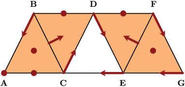
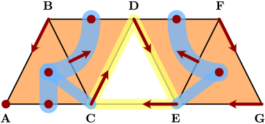
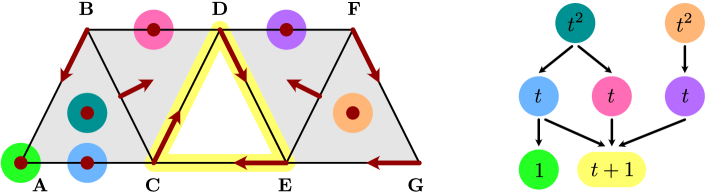
Figure 2. A Forman vector field with periodic orbit. The top left panel depicts a Forman vector field on a simplicial complex, which consists of six critical cells and eight vectors given by doubletons. Notice that the edges $\mathbf{C}\mathbf{D}$, $\mathbf{D}\mathbf{E}$, and $\mathbf{E}\mathbf{C}$ give rise to a periodic solution. In the top right panel, five connections originating in the two critical cells in dimension two are shown. While three of these connect to critical cells of dimension one, two connect to the periodic orbit. The two panels on the bottom illustrate the Morse sets of the combinatorial vector field in different colors, together with the associated Conley-Morse graph.

Example 2.6 (A Forman vector field with periodic orbit).

An example with a more elaborate Morse decomposition can be found in Figure 2. In this case, the underlying Lefschetz complex is the simplicial complex indicated in the top left panel of the figure. The multivector field $\mathcal{V}$ is actually a Forman combinatorial vector field, which consists of six critical cells, together with eight vectors given by doubletons. Of the critical cells, two have Morse index $2$, three have Morse index $1$, while only one has index $0$ — where the Morse index of a critical cell is defined as the degree of its Conley polynomial. We would like to point out that in the case of a critical cell, this polynomial is always a monomial. In addition to the critical cells, the edges $\mathbf{C}\mathbf{D}$, $\mathbf{D}\mathbf{E}$, and $\mathbf{E}\mathbf{C}$ give rise to a periodic solution. Together, these seven sets constitute the Morse sets of the minimal Morse decomposition of the vector field $\mathcal{V}$. They are indicated in different colors in the panel on the lower left. In order to get the full structure of the Morse decomposition, one needs to also determine the partial order between these Morse sets. For this, the top right panel shows five connections originating in the two critical cells in dimension two. While three of these connect to critical cells of dimension one, two connect to the periodic orbit. Similarly, one can easily determine which index $1$ critical cells connect to the periodic orbit or the vertex $\mathbf{A}$. From this, one can readily determine the Conley-Morse graph shown in the lower right panel. $\Diamond$

Intuitively, one can immediately see the connecting orbit structure of the above example, and therefore also its associated Morse decomposition. In fact, it was shown in [30] that for any Forman vector field on a simplicial complex $X$ one can explicitly construct a classical semiflow on $X$ which exhibits the same Morse sets and Conley-Morse graph. Conversely, it was shown in [29] that suitable phase space subdivisions in a classical dynamical system combined with ideas from multivector fields can be used to rigorously establish the existence of classical periodic solutions from the existence of combinatorial counterparts. These results show that the above-mentioned intuition is more than just a coincidence.

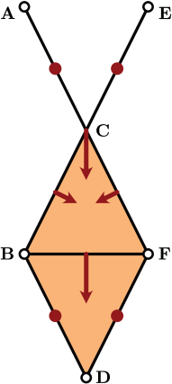
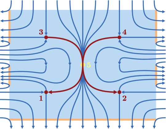
Figure 3. A multiflow without lattice of attractors. The panel on the left shows a multivector field on a Lefschetz complex, which consists of the depicted simplicial complex, but without the vertices $\mathbf{A}$, $\mathbf{B}$, $\mathbf{D}$, $\mathbf{E}$, and $\mathbf{F}$, shown as white circles. The multivector field consists of four singletons and one doubleton, as well as the multivector $\{\mathbf{C},\mathbf{B}\mathbf{C},\mathbf{C}\mathbf{F},\mathbf{B}\mathbf{C}\mathbf{F}\}$. The dynamics of this example can be represented as the multiflow shown on the right, where the only point of forward or backward nonuniqueness is the yellow point $\mathbf{5}$. For neither example one can construct a lattice of attracting sets.

Example 2.7 (A multiflow without lattice of attractors).

As our next example, consider the combinatorial multivector field presented in Figure 3(left). It is defined on the Lefschetz complex $X$ which is obtained by removing the closed subset $\{\mathbf{A},\mathbf{B},\mathbf{D},\mathbf{E},\mathbf{F}\}$ from the simplicial complex consisting of the triangles $\mathbf{B}\mathbf{C}\mathbf{F}$, $\mathbf{B}\mathbf{D}\mathbf{F}$, the edges $\mathbf{A}\mathbf{C}$, $\mathbf{C}\mathbf{E}$, and all their faces. The multivector field consists of four singleton edges and the doubleton $\{\mathbf{B}\mathbf{F},\mathbf{B}\mathbf{D}\mathbf{F}\}$, as well as the multivector $\{\mathbf{C},\mathbf{B}\mathbf{C},\mathbf{C}\mathbf{F},\mathbf{B}\mathbf{C}\mathbf{F}\}$. The singletons of the four critical edges $\mathbf{A}\mathbf{C}$, $\mathbf{B}\mathbf{D}$, $\mathbf{C}\mathbf{E}$, $\mathbf{D}\mathbf{F}$ are four isolated invariant sets. Furthermore, if we define the poset $P=\{\mathbf{p},\mathbf{q},\mathbf{r},\mathbf{s}\}$ via the Hasse diagram

(3) $$\begin{diagram}$$

and the family $\{M_{p}\}_{p\in P}$ with $M_{\mathbf{p}}:=\{\mathbf{B}\mathbf{D}\}$, $M_{\mathbf{q}}:=\{\mathbf{D}\mathbf{F}\}$, $M_{\mathbf{r}}:=\{\mathbf{A}\mathbf{C}\}$, as well as $M_{\mathbf{s}}:=\{\mathbf{C}\mathbf{E}\}$, then we obtain a well-defined Morse decomposition. Observe that all inequalities in the poset $P$ matter, because there are connections from $M_{\mathbf{r}}$ to both $M_{\mathbf{p}}$ and $M_{\mathbf{q}}$, as well as from $M_{\mathbf{s}}$ to both $M_{\mathbf{p}}$ and $M_{\mathbf{q}}$. For instance,

$$\gamma=\overleftarrow{\mathbf{A}\mathbf{C}}\cdot\mathbf{C}\cdot\mathbf{B}\mathbf{C}\mathbf{F}\cdot\mathbf{B}\mathbf{F}\cdot\mathbf{B}\mathbf{D}\mathbf{F}\cdot\overrightarrow{\mathbf{B}\mathbf{D}}$$

is an essential solution and a connection from $M_{\mathbf{r}}$ to $M_{\mathbf{p}}$. A multiflow counterpart of this example is presented in Figure 3(right). Its four saddle points are the stationary points marked in the figure as $\mathbf{1}$, $\mathbf{2}$, $\mathbf{3}$, and $\mathbf{4}$. The only point of non-uniqueness of solutions is the yellow point marked $\mathbf{5}$. Similarly to the combinatorial case, there are connections through this point from the saddle $\mathbf{3}$ to both saddles $\mathbf{1}$ and $\mathbf{2}$, as well as from saddle $\mathbf{4}$ to both saddles $\mathbf{1}$ and $\mathbf{2}$. $\Diamond$

After this sequence of examples, we return to our general discussion of Morse decompositions. Consider the family of down sets in the poset $P$, that is, the subsets $I\subset P$ such that with every $p\in I$ also all elements below $p$ are contained in $I$. We denote this family as $\mbox{$\operatorname{Down}$}(P)$. It is easy to see that $\mbox{$\operatorname{Down}$}(P)$ is a lattice of sets, which means that it is closed under union and intersection. We now associate with every $I\in\mbox{$\operatorname{Down}$}(P)$ the set $M_{I}$ consisting of all right endpoints of a path with left endpoint in the union $\bigcup_{r\in I}M_{r}$. One can check that the so-defined set $M_{I}$ is an attractor. However, the family of all such attractors is not a lattice in general, because the intersection of two attractors does not need to be an attractor itself.

In the classical setting of flows or semiflows it is possible to overcome this difficulty by constructing an attracting neighborhood $N_{I}$ for each attractor $M_{I}$ in such a way that the family $\{\,N_{I}\mid I\in\mbox{$\operatorname{Down}$}(P)\,\}$ is again a lattice, and such that the map $I\mapsto N_{I}$ is a lattice homomorphism, i.e., it preserves unions and intersections. In addition, the attracting neighborhoods $N_{I}$ have to be constructed in such a way that $M_{I}$ is the largest invariant set in $N_{I}$. In other words, the attracting set $N_{I}$ determines the attractor $M_{I}$. In the classical setting, this lattice $\{N_{I}\mid I\in\mbox{$\operatorname{Down}$}(P)\}$ is then used to proceed with the construction of the connection matrix. However, as the following example indicates, such a lattice and associated lattice homomorphism may not exist in the case of a multiflow and, similarly, in the case of a combinatorial multivector field which is inherently multivalued.

Example 2.8 (A multiflow without lattice of attractors, continued).

Consider again the multivector field and associated multiflow shown in Figure 3, which were already discussed in Example 2.7. In both of these cases, the Morse decomposition is indexed by the same poset $P=\{\mathbf{p},\mathbf{q},\mathbf{r},\mathbf{s}\}$ with Hasse diagram (3). One can easily see that the lattice of down sets of this poset is given by $\{\varnothing,\{\mathbf{p}\},\{\mathbf{q}\},\{\mathbf{p},\mathbf{q}\},\{\mathbf{p},\mathbf{q},\mathbf{r}\},\{\mathbf{p},\mathbf{q},\mathbf{s}\},P\}$. First observe that in the combinatorial case $A:=X\setminus\{\mathbf{A}\mathbf{C},\mathbf{C}\mathbf{E}\}$ does not admit an essential solution in $A$ through $\mathbf{C}$, $\mathbf{B}\mathbf{C}$, $\mathbf{C}\mathbf{F}$, and $\mathbf{B}\mathbf{C}\mathbf{F}$. Therefore, $A$ is not an isolated invariant set and, in consequence, not an attractor. Notice, however, that $M_{\{\mathbf{p},\mathbf{q},\mathbf{r}\}}\cap M_{\{\mathbf{p},\mathbf{q},\mathbf{s}\}}=A$. Hence, $\{\,M_{I}\mid I\in\mbox{$\operatorname{Down}$}(P)\,\}$ is not a lattice in this case. We claim that the above-mentioned work-around for flows with the lattice of attracting neighborhoods $N_{I}$ does not work in our combinatorial example. More precisely, there exists no lattice homomorphism which sends each down set $I$ to an attracting set $N_{I}$ for the corresponding attractor, and such that $M_{I}$ is the largest invariant subset of $N_{I}$. To show this, assume to the contrary that $I\mapsto N_{I}$ is such a homomorphism. Then one immediately obtains

$$\mathbf{C}\in M_{\{\mathbf{p},\mathbf{q},\mathbf{r}\}}\cap M_{\{\mathbf{p},\mathbf{q},\mathbf{s}\}}\subset N_{\{\mathbf{p},\mathbf{q},\mathbf{r}\}}\cap N_{\{\mathbf{p},\mathbf{q},\mathbf{s}\}}=N_{\{\mathbf{p},\mathbf{q}\}}=N_{\{\mathbf{p}\}}\cup N_{\{\mathbf{q}\}}.$$

Suppose now that we have $\mathbf{C}\in N_{\{\mathbf{p}\}}$. Since $\mathbf{C}\cdot\mathbf{B}\mathbf{C}\mathbf{F}\cdot\mathbf{B}\mathbf{F}\cdot\mathbf{B}\mathbf{D}\mathbf{F}\cdot\mathbf{D}\mathbf{F}$ is a path from $\mathbf{C}$ to $\mathbf{D}\mathbf{F}$, and since $N_{\{\mathbf{p}\}}$ is an attracting set, this implies the inclusion $\mathbf{D}\mathbf{F}\in N_{\{\mathbf{p}\}}$ — and therefore $\{\mathbf{B}\mathbf{D},\mathbf{D}\mathbf{F}\}$ is an invariant subset of $N_{\{\mathbf{p}\}}$. Yet, this is not possible, since we assumed that $M_{\{\mathbf{p}\}}=\{\mathbf{B}\mathbf{D}\}$ is the largest invariant subset of $N_{\{\mathbf{p}\}}$. Analogously one can rule out $\mathbf{C}\in N_{\{\mathbf{q}\}}$. Altogether this indeed proves that such a lattice homomorphism does not exist. The argument for the multiflow is similar. $\Diamond$

2.3. Acyclic partitions of Lefschetz complexes

Before we explain how the problem with lattices of attracting sets indicated in the previous section can be addressed, we will first consider the special case when the family of attractors $\{\,M_{I}\mid I\in\mbox{$\operatorname{Down}$}(P)\,\}$ is indeed a lattice and $I\mapsto M_{I}$ is a lattice homomorphism. One can show that in the combinatorial setting an attractor is always an attracting set of itself. Thus, in this case we also have a lattice of attracting sets — and this puts us in the setting when the approach of [14, 35] works. Actually, in view of the closedness of attracting sets, we may consider an arbitrary sublattice $\mathcal{L}$ of the lattice of closed sets in a Lefschetz complex $X$. Given a set $L\in\text{$\mathcal{L}$}$, consider now the union of all proper subsets of $L$ in $\mathcal{L}$, and denote it by $L^{\star}$. If the inequality $L^{\star}\neq L$ holds, then we call $L$ join-irreducible. Clearly, the set difference $L^{\circ}:=L\setminus L^{\star}$ is locally closed, as a difference of two closed sets. Moreover, one can in fact prove that the family $\mbox{$\operatorname{AP}$}(\text{$\mathcal{L}$}):=\mbox{$\{\,L^{\circ}\mid\text{$L$ is join-irreducible}\,\}$}$ is a partition of $X$, which in addition is acyclic in the sense that the transitive closure of the relation $L_{1}^{\circ}\preceq L_{2}^{\circ}$ defined by $L_{1}^{\circ}\cap\operatorname{cl}L_{2}^{\circ}\neq\varnothing$ makes $\mbox{$\operatorname{AP}$}(\text{$\mathcal{L}$})$ into a poset. Moreover, this resulting poset turns out to be isomorphic to the poset of join-irreducibles of $\mathcal{L}$ ordered by inclusion. Actually, the presented way of passing from a lattice of sets to an acyclic partition can be viewed as a version of the celebrated Birkhoff Theorem [5] for abstract lattices, yet for the special case of lattices of sets.

Example 2.9 (A first multivector field, continued).

For the Morse decomposition $\mathcal{M}$ discussed in Example 2.5 the lattice of down sets is given by the collection $\{\varnothing,\{\mathbf{p}\},\{\mathbf{p},\mathbf{q}\},P\}$, and one can easily see that the associated family of attractors $\text{$\mathcal{A}$}:=\{\varnothing,\{\mathbf{D}\},X\setminus\{\mathbf{A}\mathbf{B}\mathbf{C}\},X\}$ forms a lattice. Moreover, each attractor except the empty set is join-irreducible. Thus, in this case the corresponding acyclic partition $\mbox{$\operatorname{AP}$}(\text{$\mathcal{A}$})$ of $X$ coincides with the family $\mathcal{M}$ of Morse sets, and the mapping $P\ni p\mapsto M_{p}\in\mbox{$\operatorname{AP}$}(\text{$\mathcal{A}$})$ is indeed an order isomorphism. $\Diamond$

As we explain in Section 2.4 and in detail in Section 6.1, an acyclic partition of a Lefschetz complex may be used to define a connection matrix. Unfortunately, as we indicated in the previous section, the family of attractors $\{\,M_{I}\mid I\in\mbox{$\operatorname{Down}$}(P)\,\}$ may not be a lattice in the combinatorial setting. Therefore, in order to obtain the required acyclic partition we have to modify the presented approach. First observe that given an arbitrary family $\mathcal{U}$ of subsets of $X$, there is a smallest lattice of subsets of $X$ containing $\mathcal{U}$. We refer to it as the lattice extension of $\mathcal{U}$ and denote it by $\text{$\mathcal{U}$}^{\prime}$. One can easily verify that if $\mathcal{U}$ is a finite family of closed sets, then so is its lattice extension. Since, clearly, the union and intersection of attracting sets is again an attracting set, the lattice extension $\text{$\mathcal{A}$}^{\prime}$ of the family of attractors given by $\text{$\mathcal{A}$}:=\mbox{$\{\,M_{I}\mid I\in\mbox{$\operatorname{Down}$}(P)\,\}$}$ is a lattice of attracting sets. Hence, we can in fact construct a lattice, but it is no longer indexed by the down sets of the original poset $P$. Nevertheless, one can show that the acyclic partition $\text{$\mathcal{D}$}:=\mbox{$\operatorname{AP}$}(\text{$\mathcal{A}$}^{\prime})$, considered as a poset, is order isomorphic to an extension $\hat{P}$ of the original poset $P$. This enables us to write the family $\mathcal{D}$ in the form $\text{$\mathcal{D}$}=\{D_{p}\}_{p\in\hat{P}}$ where $\hat{P}\ni p\mapsto D_{p}\in\text{$\mathcal{D}$}$ is the mentioned order isomorphism. Note that every element $D_{p}$ for $p\in\hat{P}$, as a locally closed subset of the Lefschetz complex $X$, is itself a Lefschetz complex. Moreover, one can deduce from the definition of Morse decomposition that $H(D_{p})=0$ for all $p\in\hat{P}\setminus P$. This observation will then let us get rid of the elements in the set difference $\hat{P}\setminus P$ via an equivalence relation introduced in the final, algebraic step of our construction. Moreover, it turns out that instead of searching for the lattice extension $\text{$\mathcal{A}$}^{\prime}$ and the associated partition, we can just take a refined acyclic partition $\mathcal{D}$ consisting of all Morse sets together with all the multivectors not contained in a Morse set. It is not difficult to see that such multivectors must be regular. Therefore, although this may lead to an acyclic partition indexed by a larger poset, the partition elements are explicitly given and we may get rid of the elements in  $\hat{P}$ coming from the regular multivectors outside Morse sets by the the same algebraic equivalence. In fact, this straightforward construction replaces the laborious and generally not possible step (ii) of the connection matrix pipeline discussed in the introduction.

Example 2.10 (A multiflow without lattice of attractors, continued).

As we pointed out in Example 2.8 the intersection $A=M_{\{\mathbf{p},\mathbf{q},\mathbf{r}\}}\cap M_{\{\mathbf{p},\mathbf{q},\mathbf{s}\}}$ is not an attractor which implies that the family of attractors is not a lattice. Actually, in this example $A$ is the only set in the lattice extension $\text{$\mathcal{A}$}^{\prime}$ of the family of attractors $\mathcal{A}$ which is not an attractor. The set $A$ is join-irreducible in this lattice, therefore it provides

$$A^{\circ}=\{\mathbf{C},\mathbf{B}\mathbf{C},\mathbf{C}\mathbf{F},\mathbf{B}\mathbf{F},\mathbf{B}\mathbf{C}\mathbf{F},\mathbf{B}\mathbf{D}\mathbf{F}\}$$

to the associated acyclic partition $\mbox{$\operatorname{AP}$}(\text{$\mathcal{A}$}^{\prime})$. However, $A^{\circ}$ splits as the disjoint union of two multivectors $V_{1}:=\{\mathbf{C},\mathbf{B}\mathbf{C},\mathbf{C}\mathbf{F},\mathbf{B}\mathbf{C}\mathbf{F}\}$ and $V_{2}:=\{\mathbf{B}\mathbf{F},\mathbf{B}\mathbf{D}\mathbf{F}\}$. Therefore, we may take as the acyclic partition family

$$\text{$\mathcal{E}$}:=\{\,\{\mathbf{A}\mathbf{C}\},\{\mathbf{C}\mathbf{E}\},\{\mathbf{B}\mathbf{D}\},\{\mathbf{D}\mathbf{F}\},V_{1},V_{2}\,\},$$

which consists of the four singleton Morse sets and the two regular multivectors $V_{1}$ and $V_{2}$. To write it as an indexed family $\{E_{p}\}_{p\in\hat{P}}$, we take the extended poset $\hat{P}$ as the union $P\cup\{\mathbf{t},\mathbf{u}\}$ with partial order given by the Hasse diagram

$$\begin{diagram}.$$

Moreover, we define $E_{p}$ as the Morse set $M_{p}$ for $p\in P$, and additionally let $E_{\mathbf{t}}:=V_{1}$ and $E_{\mathbf{u}}:=V_{2}$. $\Diamond$

2.4. Algebraic connection matrices

The acyclic partition $\{D_{p}\}_{p\in\hat{P}}$ of the Lefschetz complex $X$ discussed in the previous section lets us decompose the associated chain complex $C(X)$ as a direct sum $C(X)=\bigoplus_{p\in\hat{P}}C(D_{p})$. It turns out that the order isomorphism $p\mapsto D_{p}$ gives this direct sum the special structure of a poset filtered chain complex, which in turn leads directly to a purely algebraic concept of connection matrix. This will be explained in more detail in the following.

We first explain the case when $\hat{P}=P$ is fixed. In terms of applications to dynamics this corresponds to the situation when we have a lattice of attracting sets indexed by down sets of the original poset in the Morse decomposition. Recall that we assume field coefficients for all considered modules, in particular chain complexes and homology modules. Given a chain complex $(C,d)$ together with a direct sum decomposition

(4) $$C=\bigoplus_{p\in P}C_{p}$$

and a down set $I\in\mbox{$\operatorname{Down}$}(P)$ we introduce the abbreviation $C_{I}:=\bigoplus_{p\in I}C_{p}$. We say that the boundary homomorphism $d$ is filtered if $d(C_{I})\subset C_{I}$ is satisfied for every $I\in\mbox{$\operatorname{Down}$}(P)$. If this is the case, then the chain complex $(C,d)$ together with the decomposition (4) is called a $P$-filtered chain complex. Similarly, any homomorphism, and in particular, any chain map $h:C\to C^{\prime}$ between two $P$-filtered chain complexes, is called filtered if

(5) $$h(C_{I})\subset C^{\prime}_{I}\quad\text{ for every }\quad I\in\mbox{$\operatorname{Down}$}(P).$$

We would like to point out that every acyclic partition $\mathcal{E}$ of a Lefschetz complex $X$ makes $C(X)$, the chain complex of $X$, a filtered chain complex via the decomposition

$$C(X)=\bigoplus_{E\in\text{$\mathcal{E}$}}C(E).$$

The decomposition is well-defined, because each $E\in\text{$\mathcal{E}$}$, as a locally closed subset of $X$, is itself a Lefschetz complex, and the fact that the boundary homomorphism is filtered may be concluded from the assumption that the partition is acyclic, see also Proposition 6.2.

Now, two $P$-filtered chain complexes are filtered chain homotopic if there exist filtered chain maps $h:C\to C^{\prime}$ and $h^{\prime}:C^{\prime}\to C$ such that the composition $h^{\prime}h$ is filtered chain homotopic to $\operatorname{id}_{C}$, and $hh^{\prime}$ is filtered chain homotopic to $\operatorname{id}_{C^{\prime}}$. In this context, a filtered chain homotopy is a chain homotopy which is itself filtered as a homomorphism. Robbin and Salamon [35] prove that every $P$-filtered chain complex is $P$-filtered chain homotopic to a reduced filtered chain complex, that is, a filtered chain complex $(C^{\prime},d^{\prime})$ such that $d^{\prime}_{pp}=0$ for all $p\in P$. Moreover, Harker, Mischaikow, and Spendlove [14] prove that if $(C,d)$ is also filtered chain homotopic to another reduced filtered complex $(C^{\prime\prime},d^{\prime\prime})$, then the filtered chain complexes $(C^{\prime},d^{\prime})$ and $(C^{\prime\prime},d^{\prime\prime})$ are in fact filtered isomorphic. Hence, up to filtered chain isomorphism every filtered chain complex has exactly one reduced representative. By definition, this representative is called its Conley complex, and the matrix of the boundary operator of the Conley complex is referred to as its connection matrix.

Example 2.11 (An algebraic example).

Consider free module $C=R\langle X\rangle$ spanned by the set of symbols

$$X:=\{\mathbf{A},\mathbf{B},\mathbf{a},\mathbf{b},\mathbf{c},{\boldsymbol{\alpha}}\}$$

and with partition $X=X_{0}\cup X_{1}\cup X_{2}$ given by

$$X_{0}:=\{\mathbf{A},\mathbf{B}\},\quad X_{1}:=\{\mathbf{a},\mathbf{b},\mathbf{c}\},\quad X_{2}:=\{{\boldsymbol{\alpha}}\}.$$

This partition lets us treat the free module $C$ as a $\mathbb{Z}$-graded module with gradation $C=\bigoplus_{i=0}^{2}R\langle X_{i}\rangle$. In order to make $C$ a free chain complex we assume that $R$ is the field $\mbox{$\mathbb{Z}$}_{2}$ and consider a homomorphism $d:C\to C$ defined on the basis $X$ by the matrix

$$\begin{array}[]{c||cccc|c|c|}d&\mathbf{A}&\mathbf{B}&\mathbf{a}&\mathbf{c}&\mathbf{b}&{\boldsymbol{\alpha}}\\ \hline\cr\hline\cr\mathbf{A}&&&1&1&1&\\ \mathbf{B}&&&1&1&1&\\ \mathbf{a}&&&&&&1\\ \mathbf{c}&&&&&&\\ \hline\cr\mathbf{b}&&&&&&1\\ \hline\cr{\boldsymbol{\alpha}}&&&&&&\\ \hline\cr\end{array}\;.$$

It is not difficult to check that $(C,d)$ is indeed a free chain complex. Furthermore, it can be made into a poset filtered chain complex by considering the poset $P:=\{\mathbf{p},\mathbf{q},\mathbf{r}\}$ linearly ordered by $\mathbf{p}<\mathbf{q}<\mathbf{r}$ and setting

$$C_{\mathbf{p}}:=R\langle\{\mathbf{A},\mathbf{B},\mathbf{a},\mathbf{c}\}\rangle,\quad C_{\mathbf{q}}:=R\langle\{\mathbf{b}\}\rangle,\quad C_{\mathbf{r}}:=R\langle\{{\boldsymbol{\alpha}}\}\rangle.$$

Again, one can easily check that the gradation $C=\bigoplus_{p\in P}C_{p}$ turns $(C,d)$ into a $P$-filtered chain complex. Since we have $d_{\mathbf{p}\mathbf{p}}\neq 0$, this complex $C$ is not reduced.

One can also consider a submodule $\bar{C}$ of $C$ which is obtained by removing the generators $\mathbf{B}$ and $\mathbf{c}$, i.e., we have

$$\bar{C}_{\mathbf{p}}:=R\langle\{\mathbf{A},\mathbf{a}\}\rangle,\quad\bar{C}_{\mathbf{q}}:=R\langle\{\mathbf{b}\}\rangle,\quad\bar{C}_{\mathbf{r}}:=R\langle\{{\boldsymbol{\alpha}}\}\rangle,$$

together with the boundary homomorphism $\bar{d}:\bar{C}\to\bar{C}$ given by the matrix

$$\begin{array}[]{c||cc|c|c|}\bar{d}&\mathbf{A}&\mathbf{a}&\mathbf{b}&{\boldsymbol{\alpha}}\\ \hline\cr\hline\cr\mathbf{A}&&&&\\ \mathbf{a}&&&&1\\ \hline\cr\mathbf{b}&&&&1\\ \hline\cr{\boldsymbol{\alpha}}&&&&\\ \hline\cr\end{array}\;.$$

We leave it to the reader to verify that this indeed defines a $P$-filtered complex $(\bar{C},\bar{d})$. Furthermore, this chain complex is reduced and, in fact, is a Conley complex of $(C,d)$ which makes the matrix of $\bar{d}$ a connection matrix of $(C,d)$. To see this in more detail, consider the two specific homomorphisms $h:C\to\bar{C}$ and $g:\bar{C}\to C$ given by the matrices

$$\begin{array}[]{c||cccc|c|c|}h&\mathbf{A}&\mathbf{B}&\mathbf{a}&\mathbf{c}&\mathbf{b}&{\boldsymbol{\alpha}}\\ \hline\cr\hline\cr\mathbf{A}&1&1&&&&\\ \mathbf{a}&&&1&&&\\ \hline\cr\mathbf{b}&&&&&1&\\ \hline\cr{\boldsymbol{\alpha}}&&&&&&1\\ \hline\cr\end{array}\qquad\text{ and }\qquad\begin{array}[]{c||cc|c|c|}g&\mathbf{A}&\mathbf{a}&\mathbf{b}&{\boldsymbol{\alpha}}\\ \hline\cr\hline\cr\mathbf{A}&1&&&\\ \mathbf{B}&&&&\\ \mathbf{a}&&1&&\\ \mathbf{c}&&1&1&\\ \hline\cr\mathbf{b}&&&1&\\ \hline\cr{\boldsymbol{\alpha}}&&&&1\\ \hline\cr\end{array}\;.$$

One can immediately verify that both $g$ and $h$ are indeed $P$-filtered chain maps, and that the identity $h\circ g=\operatorname{id}_{\bar{C}}$ is satisfied. Moreover, the composition $g\circ h$ can be computed as the matrix

$$\begin{array}[]{c||cccc|c|c|}g\circ h&\mathbf{A}&\mathbf{B}&\mathbf{a}&\mathbf{c}&\mathbf{b}&{\boldsymbol{\alpha}}\\ \hline\cr\hline\cr\mathbf{A}&1&1&&&&\\ \mathbf{B}&&&&&&\\ \mathbf{a}&&&1&&&\\ \mathbf{c}&&&1&&1&\\ \hline\cr\mathbf{b}&&&&&1&\\ \hline\cr{\boldsymbol{\alpha}}&&&&&&1\\ \hline\cr\end{array}\;.$$

Therefore, this composition $g\circ h$ is filtered chain homotopic to $\operatorname{id}_{C}$ via the $P$-filtered chain homotopy $\gamma:C\to C$ which sends all generators to zero, except $\mathbf{B}$ which is sent to $\mathbf{c}$. In fact, this chain homotopy is an example of an elementary reduction via the pair of generators $(\mathbf{B},\mathbf{c})$ discussed in [16, Section 4.3], see also [17]. We presented this example purely algebraically, but in fact its algebra provides the connection matrix for the Morse decomposition of a combinatorial multivector field which we will discuss in more detail in Example 2.14 below. $\Diamond$

As we mentioned already earlier, one has to modify this definition to accommodate the situation when we cannot keep the original poset $P$ as in Examples 2.7, 2.8, and 2.10. Under a changing poset the condition (5) in the definition of a filtered homomorphism needs to be modified. For this, let $P$ and $P^{\prime}$ be two posets and consider a $P$-filtered chain complex $(C,d)$, as well as a $P^{\prime}$-filtered chain complex $(C^{\prime},d^{\prime})$. In order to speak about a filtered homomorphism in this setting we need a way to relate down sets in the two posets $P$ and $P^{\prime}$. Note that if $\alpha:P^{\prime}\to P$ is order preserving, then we have $\alpha^{-1}(I)\in\mbox{$\operatorname{Down}$}(P^{\prime})$ for every $I\in\mbox{$\operatorname{Down}$}(P)$. Therefore, we can define a morphism from a $P$-filtered chain complex $(C,d)$ to a $P^{\prime}$-filtered chain complex $(C^{\prime},d^{\prime})$ as a pair ($\alpha,h)$ where $\alpha:P^{\prime}\to P$ is order preserving and $h:C\to C^{\prime}$ is a chain map satisfying

(6) $$h(C_{I})\subset C^{\prime}_{\alpha^{-1}(I)}\quad\text{ for every }\quad I\in\mbox{$\operatorname{Down}$}(P).$$

A similar modification allows us to also extend the definition of filtered chain homotopy to the setting of varying posets.

We still need some further modifications to guarantee that in this algebraic step we can eliminate the elements added to the poset to obtain a lattice of attracting sets. For this, recall that subcomplexes $C_{p}$ for the added values of $p$ are Lefschetz complexes with zero homology or, equivalently, they are chain homotopic to zero. Therefore, if $\bar{C}$ denotes the Conley complex of $C$ computed under a fixed poset $P$, the chain groups $\bar{C}_{p}$ for an added element $p$ are zero. In consequence, the respective rows and columns in the connection matrix are empty, because the only basis of the zero group is empty. To formalize the removal of these empty rows and columns we do four things:

• We add a distinguished subset $P_{\star}\subset P$ and require that all chain groups $C_{p}$ for $p\in P\setminus P_{\star}$ are chain homotopic to zero.

• We extend the definition of a reduced chain complex by additionally requesting that $P_{\star}=P$ in a reduced complex.

• We allow partial order preserving maps $\alpha:P^{\prime}\nrightarrow P$ to relate down sets in the posets $P$ and $P^{\prime}$, but we require that $\alpha$ is defined at least for all $p^{\prime}\in P^{\prime}_{\star}$. The partial map $\alpha$ does not need to be defined for elements $p^{\prime}\in P^{\prime}\setminus P^{\prime}_{\star}$, since a term $\bar{C}^{\prime}_{p}=0$ in the Conley complex contributes nothing to the whole Conley complex.

• Finally, since the preimage $\alpha^{-1}(I)$ for $I\in\mbox{$\operatorname{Down}$}(P)$ no longer needs to be a down set under a partially defined order preserving map, we also have to replace (6) by the condition

  (7) $$h(C_{I})\subset C^{\prime}_{\alpha^{-1}(I)^{\leq}}\quad\text{ for every }\quad I\in\mbox{$\operatorname{Down}$}(P),$$

  where $A^{\leq}$ denotes the smallest down set containing $A$, for $A\subset P^{\prime}$. We refer to chain maps satisfying (7) as $\alpha$-filtered.

Summarizing, the above extensions lead to a well-defined category PfCc whose objects are of the form $(P,C,d)$, where $P$ is a poset with a distinguished subset $P_{\star}$ and $(C,d)$ is a $P$-filtered chain complex. In addition, morphisms from $(P,C,d)$ to $(P^{\prime},C^{\prime},d^{\prime})$ are of the form $(\alpha,h)$, where $\alpha:P^{\prime}\nrightarrow P$ is a partial order preserving map whose domain contains $P^{\prime}_{\star}$ and which satisfies $\alpha(P^{\prime}_{\star})\subset P_{\star}$, and $h:C\to C^{\prime}$ is a chain map satisfying (7). As it turns out, the main results of [14, 35] can be extended to this new category. More precisely, we prove later in the paper the following result.

Theorem 2.12 (Existence of the Conley complex and connection matrix).

Consider the category PfCc of poset filtered chain complexes with varying posets introduced above. Then the following hold:

• Every object in PfCc is filtered chain homotopic to a reduced object.

• If two reduced objects in PfCc are filtered chain homotopic, then they automatically are isomorphic in PfCc.

In other words, up to isomorphism every object in PfCc has exactly one reduced representative, which is called its Conley complex. The matrix of the boundary operator of the Conley complex is called connection matrix.

The above result provides both the Conley complex and the connection matrix also in the case when there is no lattice homomorphism from down sets in the poset of a Morse decomposition to attracting sets in this Morse decomposition, as discussed earlier. A bonus, which comes as a side effect, is that we can take a shortcut in the connection matrix pipeline by skipping the construction of the lattice of attracting neighborhoods and passing immediately from the Morse decomposition in step (i) to a filtered chain complex in step (iii) via an acyclic partition of the phase space associated with the Morse decomposition under the extended poset.

Example 2.13 (A multiflow without lattice of attractors, continued).

Consider the acyclic partition $\text{$\mathcal{E}$}=\{E_{p}\}_{p\in\hat{P}}$ introduced in Example 2.10, which corresponds to the Morse decomposition of the multivector field on the Lefschetz complex $X$ in Figure 3(left). The boundary homomorphism $d$ of the associated chain complex $C(X)$ of $X$ has the matrix

$$\begin{array}[]{c||c|c|cc|cccc|c|c||}d&\mathbf{B}\mathbf{D}&\mathbf{D}\mathbf{F}&\mathbf{B}\mathbf{F}&\mathbf{B}\mathbf{D}\mathbf{F}&\mathbf{C}&\mathbf{B}\mathbf{C}&\mathbf{C}\mathbf{F}&\mathbf{B}\mathbf{C}\mathbf{F}&\mathbf{A}\mathbf{C}&\mathbf{C}\mathbf{E}\\ \hline\cr\hline\cr\mathbf{B}\mathbf{D}&&&&1&&&&&&\\ \hline\cr\mathbf{D}\mathbf{F}&&&&1&&&&&&\\ \hline\cr\mathbf{B}\mathbf{F}&&&&1&&&&1&&\\ \mathbf{B}\mathbf{D}\mathbf{F}&&&&&&&&&&\\ \hline\cr\mathbf{C}&&&&&&1&1&&1&1\\ \mathbf{B}\mathbf{C}&&&&&&&&1&&\\ \mathbf{C}\mathbf{F}&&&&&&&&1&&\\ \mathbf{B}\mathbf{C}\mathbf{F}&&&&&&&&&&\\ \hline\cr\mathbf{A}\mathbf{C}&&&&&&&&&&\\ \hline\cr\mathbf{C}\mathbf{E}&&&&&&&&&&\\ \hline\cr\end{array}\;.$$

One can immediately verify that $(C(X),d)$ gives a $\hat{P}$-filtered chain complex. For $p\in\hat{P}\setminus P=\{\mathbf{t},\mathbf{u}\}$ the induced Lefschetz complex $X_{p}$ is chain homotopic to zero. Therefore, we take $\hat{P}_{*}:=P$ as the distinguished subset in $\hat{P}$. This way we obtain an object $(\hat{P},C(X),d)$ of PfCc. We note that $d$ is not reduced, because $d_{\mathbf{t}\mathbf{t}}\neq 0$, $d_{\mathbf{u}\mathbf{u}}\neq 0$ and, additionally, $C(X_{p})$ is chain homotopic to zero for $p\in\hat{P}\setminus P$.

Consider now the free module $R\langle\mathbf{B}\mathbf{D},\mathbf{D}\mathbf{F},\mathbf{A}\mathbf{C},\mathbf{C}\mathbf{E}\rangle$ and turn it into a chain complex $\bar{C}$ by assuming the boundary map to be zero. Clearly, the definitions $\bar{C}_{\mathbf{p}}:=\langle\mathbf{B}\mathbf{D}\rangle$, $\bar{C}_{\mathbf{q}}:=\langle\mathbf{D}\mathbf{F}\rangle$, $\bar{C}_{\mathbf{r}}:=\langle\mathbf{A}\mathbf{C}\rangle$, and $\bar{C}_{\mathbf{s}}:=\langle\mathbf{C}\mathbf{E}\rangle$ render $\bar{C}$ a $P$-filtered chain complex. After finally letting $\bar{P}:=\bar{P}_{\star}:=P$, we now claim that $(\bar{P},\bar{C},0)$ is a Conley complex of the Morse decomposition associated with the multivector field on the Lefschetz complex $X$ in Figure 3(left). In order to see this, let $\alpha:\bar{P}\hookrightarrow\hat{P}$ denote the inclusion map and let $\beta:\hat{P}\nrightarrow\bar{P}$ be the partial map which, as a relation, is the inverse of $\alpha$. Consider the homomorphisms $h:C(X)\to\bar{C}$ and $g:\bar{C}\to C(X)$ given by the matrices

$$\begin{array}[]{c||c|c|cc|cccc|c|c||}h&\mathbf{B}\mathbf{D}&\mathbf{D}\mathbf{F}&\mathbf{B}\mathbf{F}&\mathbf{B}\mathbf{D}\mathbf{F}&\mathbf{C}&\mathbf{B}\mathbf{C}&\mathbf{C}\mathbf{F}&\mathbf{B}\mathbf{C}\mathbf{F}&\mathbf{A}\mathbf{C}&\mathbf{C}\mathbf{E}\\ \hline\cr\hline\cr\mathbf{B}\mathbf{D}&1&&1&&&&1&&&\\ \hline\cr\mathbf{D}\mathbf{F}&&1&1&&&&1&&&\\ \hline\cr\mathbf{A}\mathbf{C}&&&&&&&&&1&\\ \hline\cr\mathbf{C}\mathbf{E}&&&&&&&&&&1\\ \hline\cr\end{array}$$

and

$$\begin{array}[]{c||c|c|c|c||}g&\mathbf{B}\mathbf{D}&\mathbf{D}\mathbf{F}&\mathbf{A}\mathbf{C}&\mathbf{C}\mathbf{E}\\ \hline\cr\hline\cr\mathbf{B}\mathbf{D}&1&&&\\ \hline\cr\mathbf{D}\mathbf{F}&&1&&\\ \hline\cr\mathbf{B}\mathbf{F}&&&&\\ \mathbf{B}\mathbf{D}\mathbf{F}&&&&\\ \hline\cr\mathbf{C}&&&&\\ \mathbf{B}\mathbf{C}&&&1&1\\ \mathbf{C}\mathbf{F}&&&&\\ \mathbf{B}\mathbf{C}\mathbf{F}&&&&\\ \hline\cr\mathbf{A}\mathbf{C}&&&1&\\ \hline\cr\mathbf{C}\mathbf{E}&&&&1\\ \hline\cr\end{array}\;.$$

One can immediately verify that $h$ is an $\alpha$-filtered chain map, and that $g$ is a $\beta$-filtered chain map. Hence, both $(\alpha,h)$ and $(\beta,g)$ are morphisms in PfCc. It turns out that $(\alpha,h)\circ(\beta,g)=\operatorname{id}_{(\bar{P},\bar{C},0)}$, and that $(\beta,g)\circ(\alpha,h)$ is filtered chain homotopic to $\operatorname{id}_{(\hat{P},C(X),d)}$ via a $\hat{P}$-filtered homotopy $\gamma:C(X)\to C(X)$ defined by the matrix

$$\begin{array}[]{c||c|c|cc|cccc|c|c||}\gamma&\mathbf{B}\mathbf{D}&\mathbf{D}\mathbf{F}&\mathbf{B}\mathbf{F}&\mathbf{B}\mathbf{D}\mathbf{F}&\mathbf{C}&\mathbf{B}\mathbf{C}&\mathbf{C}\mathbf{F}&\mathbf{B}\mathbf{C}\mathbf{F}&\mathbf{A}\mathbf{C}&\mathbf{C}\mathbf{E}\\ \hline\cr\hline\cr\mathbf{B}\mathbf{D}&&&&&&&&&&\\ \hline\cr\mathbf{D}\mathbf{F}&&&&&&&&&&\\ \hline\cr\mathbf{B}\mathbf{F}&&&&&&&&&&\\ \mathbf{B}\mathbf{D}\mathbf{F}&&&1&&&&1&&&\\ \hline\cr\mathbf{C}&&&&&&&&&&\\ \mathbf{B}\mathbf{C}&&&&&1&&&&&\\ \mathbf{C}\mathbf{F}&&&&&&&&&&\\ \mathbf{B}\mathbf{C}\mathbf{F}&&&&&&&1&&&\\ \hline\cr\mathbf{A}\mathbf{C}&&&&&&&&&&\\ \hline\cr\mathbf{C}\mathbf{E}&&&&&&&&&&\\ \hline\cr\end{array}\;.$$

This confirms that $(\bar{P},\bar{C},0)$ is a Conley complex of the Morse decomposition associated with the multivector field on the Lefschetz complex $X$ in Figure 3(left). $\Diamond$

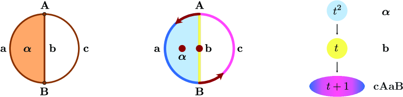
Figure 4. Small Lefschetz complex with periodic orbit. The left panel shows a small Lefschetz complex which consists of a $2$-cell $\mathbf{{\boldsymbol{\alpha}}}$, three $1$-cells $\mathbf{a}$, $\mathbf{b}$, $\mathbf{c}$, and two $0$-cells $\mathbf{A}$, $\mathbf{B}$. On this complex, we study the combinatorial vector field shown in the middle panel, which consists of two singletons and two doubletons. The associated Conley-Morse graph is shown on the right, with Morse sets given by the critical cells $\{{\boldsymbol{\alpha}}\}$ and $\{\mathbf{b}\}$, as well as the periodic orbit $\{\mathbf{c},\mathbf{A},\mathbf{a},\mathbf{B}\}$.

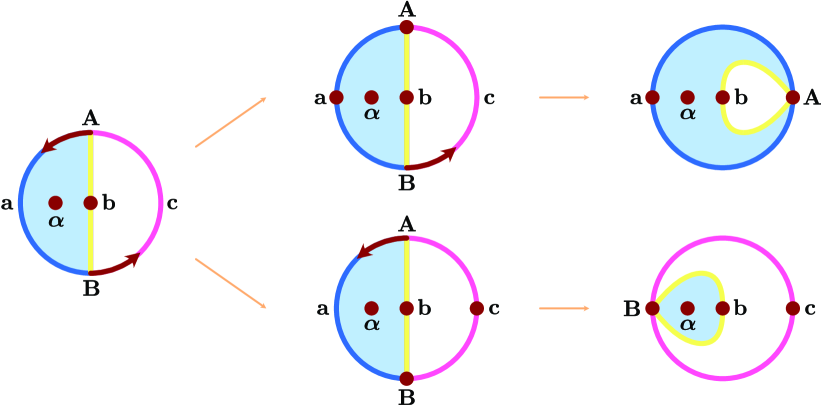
Figure 5. Small Lefschetz complex with periodic orbit. For the combinatorial vector field shown in Figure 4, the above diagram sketches the computation of two different connection matrices, based on two different elementary chain complex reductions. The top arrow sequence uses the reduction pair $(B,c)$, while the bottom sequence is for $(A,a)$. In both cases, the final chain complex is reduced and boundaryless.

We have already presented one example of a connection matrix in the context of Example 2.5. In that case, it could easily be derived from the fact that the homology of the Conley complex is isomorphic to the homology of the underlying Lefschetz complex. A more complicated example will further illustrate Theorem 2.12.

Example 2.14 (Small Lefschetz complex with periodic orbit).

As a more elaborate example, yet one that still can be discussed directly in detail, consider the Lefschetz complex $X$ shown in the left panel of Figure 4. This complex consists of a semi-circle shaped two-dimensional cell ${\boldsymbol{\alpha}}$, whose boundary consists of the vertices $\mathbf{A}$ and $\mathbf{B}$, together with the two $1$-cells $\mathbf{a}$ and $\mathbf{b}$. In addition, the complex contains a third $1$-cell $\mathbf{c}$ which joins the two vertices. On $X$ we consider the combinatorial vector field $\mathcal{V}$ sketched in the middle panel of Figure 4, and which consists of two singletons and two doubletons. The associated Conley-Morse graph is shown on the right, with Morse sets given by the critical cells $\{{\boldsymbol{\alpha}}\}$ and $\{\mathbf{b}\}$, as well as the periodic orbit $\{\mathbf{c},\mathbf{A},\mathbf{a},\mathbf{B}\}$.

	$\mathbf{A}$	$\mathbf{a}$	$\mathbf{b}$	${\boldsymbol{\alpha}}$
$\mathbf{A}$		0	0
$\mathbf{a}$				1
$\mathbf{b}$				1
${\boldsymbol{\alpha}}$

	$\mathbf{B}$	$\mathbf{c}$	$\mathbf{b}$	${\boldsymbol{\alpha}}$
$\mathbf{B}$		0	0
$\mathbf{c}$				0
$\mathbf{b}$				1
${\boldsymbol{\alpha}}$

Table 1. Small Lefschetz complex with periodic orbit. Two connection matrices for the combinatorial vector field from Figure 4. The matrix on the left is the result of the reduction process indicated via the top arrows in Figure 5, while the bottom arrows lead to the matrix shown on the right.

Due to the small size of the Lefschetz complex $X$, one can immediately reduce the associated chain complex via elementary reduction pairs. For example, if one uses the reduction pair $(B,c)$, one obtains the sequence of Lefschetz complexes shown in the top arrow sequence in Figure 5, and this leads to the connection matrix shown in Table 1(left). We discussed algebraic details of the computation of this connection matrix in Example 2.11. In contrast, if one uses the reduction pair $(A,a)$, then the sequence of Lefschetz complexes is as in the bottom arrow sequence of Figure 5, and one obtains the connection matrix in Table 1(right). The algebraic details of this computation are similar to those presented in Example 2.11. $\Diamond$

2.5. Uniqueness of connection matrices

Theorem 2.12(ii) implies that connection matrices are uniquely determined up to an isomorphism in PfCc. While this statement is clearly correct, it does not convey the complete story. This statement only means that any two connection matrices of a given filtered chain complex are similar via the matrix of a filtered chain map. However, there is also a stronger equivalence relation between connection matrices, which is important in its own right.

To explain this, recall that every Conley complex of a given filtered chain complex, considered as an object of PfCc, may be considered together with the filtered chain maps establishing the filtered chain homotopy. The composition of these filtered chain maps between the two Conley complexes of a given filtered chain complex is a filtered chain map. Nevertheless, this composition may or may not be a graded chain map, which we define as a chain map $h:C_{p}\to C^{\prime}_{p}$ such that $h(C_{p})\subset C^{\prime}_{\alpha^{-1}(p)}$. This leads to a stronger equivalence relation between connection matrices which lets us speak about uniqueness and nonuniqueness of connection matrices. In particular, one of the main results of the paper is the following theorem, whose precise formulation can be found in Theorem 8.21.

Theorem 2.15 (Unique connection matrix for gradient vector fields).

Assume that $\mathcal{V}$ is a gradient combinatorial vector field on a regular Lefschetz complex $X$. Then the Morse decomposition consisting of all the critical cells of $\mathcal{V}$ has precisely one connection matrix. It coincides with the matrix of the boundary operator of the associated Conley complex.

In addition to being unique, the connection matrix of a gradient combinatorial vector field also allows us to establish connections between Morse sets, as the following result shows. Its precise formulation is the subject of Theorem 8.22, and this result also explains how the connections can be found explicitly.

Theorem 2.16 (Existence of connecting orbits).

Assume that $\mathcal{V}$ is a gradient combinatorial vector field on a regular Lefschetz complex $X$, and let $M_{p}$ and $M_{q}$ with $p<q$ denote two critical cells of $\mathcal{V}$ such that the entry in the connection matrix corresponding to these cells is non-zero. Then there exists a connection between $M_{q}$ and $M_{p}$.

In fact, the above result under slightly stronger assumptions remains true for general multivector fields, see Theorem 7.18. We illustrate these two results in the following example.

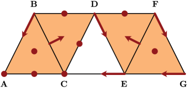
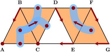
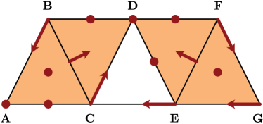
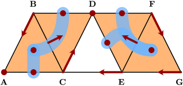
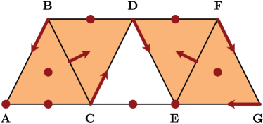
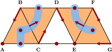
Figure 6. Three Forman gradient vector fields. The above panels show three different combinatorial Forman gradient vector fields. All of them are related to the combinatorial vector field from Figure 2, yet they destroy its periodic orbit which traverses the vertices $\mathbf{C}$, $\mathbf{D}$, and $\mathbf{E}$. This is achieved by replacing precisely one vector in the periodic orbit by two critical cells — one edge and one vertex. Since the periodic orbit consists of three vectors, there are three different ways of breaking it, leading to the vector fields in the left column. In the right column, we indicate for each case which connections exist between the index $2$ and index $1$ critical cells.

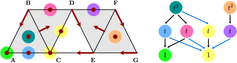
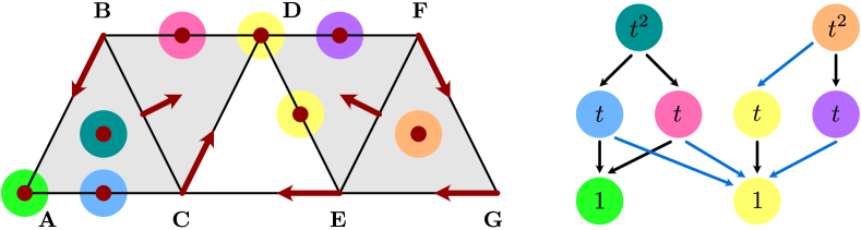
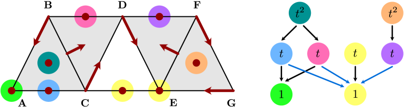
Figure 7. Three Forman gradient vector fields. For the combinatorial vector fields shown in Figure 6, the above panels depict their associated Morse decompositions. The Morse sets are indicated by different colors in the left column, while the Conley-Morse graphs are shown on the right. In each case, the two Morse sets obtained via breaking the periodic orbit in Figure 2 are shown in yellow.

	$\mathit{CD}$	$\mathbf{AC}$	$\mathbf{BD}$	$\mathbf{DF}$	$\mathbf{ABC}$	$\mathbf{EFG}$
$\mathbf{A}$	0	1	1	0
$\mathit{C}$	0	1	1	0
$\mathit{CD}$					1	0
$\mathbf{AC}$					1	0
$\mathbf{BD}$					1	0
$\mathbf{DF}$					0	1

	$\mathit{DE}$	$\mathbf{AC}$	$\mathbf{BD}$	$\mathbf{DF}$	$\mathbf{ABC}$	$\mathbf{EFG}$
$\mathbf{A}$	0	1	1	0
$\mathit{D}$	0	1	1	0
$\mathit{DE}$					0	1
$\mathbf{AC}$					1	0
$\mathbf{BD}$					1	0
$\mathbf{DF}$					0	1

	$\mathit{CE}$	$\mathbf{AC}$	$\mathbf{BD}$	$\mathbf{DF}$	$\mathbf{ABC}$	$\mathbf{EFG}$
$\mathbf{A}$	0	1	1	0
$\mathit{E}$	0	1	1	0
$\mathit{CE}$					0	0
$\mathbf{AC}$					1	0
$\mathbf{BD}$					1	0
$\mathbf{DF}$					0	1

Table 2. Three Forman gradient vector fields. For the three combinatorial vector fields shown in Figure 6 and associated Morse decompositions in Figure 7, the three unique connection matrices are listed above. Only the two right-most entries in the third row are changing, and they correspond to the connections from the index $2$ critical cells to the index $1$ critical cell on the destroyed periodic orbit. Note that the nonzero entries in the lower right $4\times 2$-submatrices correspond exactly to the connections indicated in the right column of Figure 6.

Example 2.17 (Three Forman gradient vector fields).

Consider the three combinatorial Forman vector fields shown in the left column of Figure 6. All of them are defined on the same simplicial complex, and they consist of eight critical cells and seven doubletons. In fact, one can easily see that all of these vector fields are related to the combinatorial vector field from Figure 2, which has a periodic orbit traversing the vertices $\mathbf{C}$, $\mathbf{D}$, and $\mathbf{E}$. While the latter vector field is therefore not gradient, it is possible to destroy its recurrent behavior by replacing precisely one vector in the periodic orbit by two critical cells — one edge and one vertex. Since the periodic orbit consists of three vectors, this leads to the three different gradient vector fields shown in the left column of Figure 6. Their corresponding Morse decompositions are depicted in Figure 7.

Using our results from Section 8, one can easily determine the unique connection matrix of a combinatorial gradient vector field. This basically amounts to finding suitable bases of chains in each dimension and creating the matrix of the boundary operator with respect to these bases, see the detailed description in Theorem 8.21 and Proposition 8.15. For the gradient combinatorial vector field in the last row of Figure 6 this is illustrated in detail in Example 8.23, and this leads to the last connection matrix in Table 2. For the first two gradient vector fields, their connection matrices are given by the first two matrices in Table 2, respectively, and they can be determined using the basis elements described in Example 8.13. Notice that the nonzero entries in all three of these matrices between critical cells of index $2$ and critical cells of index $1$ yield precisely the connecting orbits shown in the right column of Figure 6. Similarly, nonzero entries between critical cells of index $1$ and critical cells of index $0$ do correspond to connections in the combinatorial vector fields. Note, however, that the entry in the connection matrix records also the multiplicity of such connections. This is the reason why the connection matrices record the connections between $\mathbf{B}\mathbf{D}$ or $\mathbf{A}\mathbf{C}$ and the vertex $\mathbf{A}$, as well as with the additional critical vertex in the support of the destroyed periodic orbit. In contrast, connections originating at either $\mathbf{D}\mathbf{F}$ or the critical cell of dimension one on the former periodic orbit do not give rise to nonzero entries in the connection matrix, since in these cases the two different connections end at the same critical vertex. $\Diamond$

Example 2.18 (A Forman vector field with periodic orbit, continued).

Based on the previous example, we can now revisit the combinatorial vector field from Figure 2, which has already been discussed in Example 2.6. Notice that this vector field has a periodic orbit which traverses the vertices $\mathbf{C}$, $\mathbf{D}$, and $\mathbf{E}$. The existence of this periodic orbit makes the system non-gradient, and therefore we cannot apply Theorem 2.15 to obtain the existence of a unique connection matrix.

Nevertheless, Theorem 2.15 guarantees the existence of a connection matrix in this situation as well. In order to explain how such a matrix can be determined using the previous example, note that the Conley polynomial of the periodic orbit is given by $t+1$, i.e., the associated homology groups are one-dimensional in dimensions $0$ and $1$. In Example 2.17 we saw that by replacing a vector on the periodic orbit by one critical cell each of dimension $0$, one obtains a gradient system with a unique connection matrix. In fact, the sum of the homology groups of these newly added critical cells is isomorphic to the Conley index of the periodic orbit, and therefore one would expect that all three connection matrices from Table 2 should be connection matrices for the vector field in Figure 2. As we will see later, this is indeed the case, and thus in all three cases the nontrivial entries correspond to connections between the respective Morse sets. For a more detailed explanation we refer the reader to Example 8.24. $\Diamond$

3. Preliminaries

3.1. Sets, maps, relations, and partial orders

We denote the sets of reals, integers, positive integers, and non-negative integers by $\mathbb{R}$, $\mathbb{Z}$, $\mathbb{N}$, and $\mbox{$\mathbb{N}$}_{0}$, respectively. Given a set $X$, we write $\operatorname{card}X$ for the number of elements of $X$ and we denote the family of all subsets of $X$ by $\text{$\mathcal{P}$}(X)$. A partition of a set $X$ is a family $\text{$\mathcal{E}$}\subset\text{$\mathcal{P}$}(X)$ of mutually disjoint non-empty subsets of $X$ such that $\bigcup\text{$\mathcal{E}$}=X$. For a subfamily $\text{$\mathcal{E}$}^{\prime}\subset\text{$\mathcal{E}$}$ of a partition $\mathcal{E}$ of $X$ we will use the compact notation $|\text{$\mathcal{E}$}^{\prime}|$ to denote the union of sets in $\text{$\mathcal{E}$}^{\prime}$, that is, we define $|\text{$\mathcal{E}$}^{\prime}|=\bigcup\text{$\mathcal{E}$}^{\prime}$.

A $K$-indexed family of subsets of a given set $X$ is an injective map of the form $K\ni k\mapsto X_{k}\in\text{$\mathcal{P}$}(X)$. We denote such a family by $(X_{k})_{k\in K}$. Note that every family $\text{$\mathcal{E}$}\subset\text{$\mathcal{P}$}(X)$ may be considered as an $\mathcal{E}$-indexed family via the map $\text{$\mathcal{E}$}\ni E\mapsto E\in\text{$\mathcal{P}$}(X)$. In this case we say that $\mathcal{E}$ is a self-indexing family. By a $K$-gradation of a set $X$ we mean a $K$-indexed family $(X_{k})_{k\in K}$ such that $\{X_{k}\}_{k\in K}$ is a partition of $X$. Note, in particular, that every surjective map $f:X\to K$ induces the $K$-gradation $(f^{-1}(k))_{k\in K}$ of $X$. We refer to this $K$-gradation as the $f$-gradation of $X$. Given a subset $A\subset X$ and a gradation $(X_{k})_{k\in K}$ of $X$, the induced gradation is the gradation $(A\cap X_{k})_{k\in K_{A}}$ of $A$ where $K_{A}:=\mbox{$\{\,k\in K\mid A\cap X_{k}\neq\varnothing\,\}$}$.

We write $f:X\nrightarrow Y$ for a partial map from $X$ to $Y$, that is, a map defined on a subset $\operatorname{dom}f\subset X$, called the domain of $f$, and such that the set of values of $f$, denoted by $\operatorname{im}f$, is contained in $Y$. Partial maps are composed in the obvious way: If $f:X\nrightarrow Y$ and $g:Y\nrightarrow Z$ are partial maps, then the domain of their composition $g\circ f:X\nrightarrow Z$ is given by $\operatorname{dom}(g\circ f)=f^{-1}(\operatorname{dom}g)$, and on this domain we have $(g\circ f)(x)=g(f(x))$.

In the sequel, we work with the category of finite sets with a distinguished subset, which is denoted by DSet and defined as follows. The objects of DSet are pairs $(X,X_{\star})$, where $X$ is a finite set and $X_{\star}\subset X$ is a distinguished subset. The morphisms from $(X,X_{\star})$ to $(Y,Y_{\star})$ in DSet are subset preserving partial maps, that is, partial maps $f:X\nrightarrow Y$ such that the inclusions $X_{\star}\subset\operatorname{dom}f$ and $f(X_{\star})\subset Y_{\star}$ are satisfied. One easily verifies that DSet with the composition of morphisms defined as the composition of partial maps and the identity morphism defined as the identity map is indeed a category.

Given a set $X$ and a binary relation $R\subset X\times X$, we write $xRy$ meaning $(x,y)\in R$. The inverse of $R$, denoted $R^{-1}$, is the relation $R^{-1}:=\mbox{$\{\,(y,x)\mid xRy\,\}$}$. By the transitive closure of $R$ we mean the relation $\bar{R}\subset X\times X$ given by $x\bar{R}y$ if there exists a sequence $x=x_{0},x_{1},\ldots,x_{n}=y$ such that $n\geq 1$ and $x_{i-1}Rx_{i}$ for $i=1,2,\ldots,n$.

A multivalued map $F:X\multimap Y$ is a map $F:X\to\text{$\mathcal{P}$}(Y)$. For $A\subset X$ we define the image of $A$ by $F(A):=\bigcup\mbox{$\{\,F(x)\mid x\in A\,\}$}$ and for $B\subset Y$ we define the preimage of $B$ by $F^{-1}(B):=\mbox{$\{\,x\in X\mid F(x)\cap B\neq\varnothing\,\}$}.$

Given a relation $R$, we associate with it a multivalued map $F_{R}:X\multimap X$ via the definition $F_{R}(x):=R(x)$, where $R(x):=\mbox{$\{\,y\in X\mid xRy\,\}$}$ is the image of $x\in X$ in $R$. Obviously, $R\mapsto F_{R}$ is a one-to-one correspondence between binary relations in $X$ and multivalued maps from $X$ to $X$. Often, it will be convenient to interpret the relation $R$ as a directed graph whose set of vertices is $X$ and a directed arrow goes from $x$ to $y$ whenever $xRy$. The three concepts relation, multivalued map, and directed graph are equivalent on the formal level and the distinction is used only to emphasize different points of view. However, in this paper it will be convenient to use all these concepts interchangeably.

Recall that a partial order in a set $P$ is a reflexive, antisymmetric and transitive relation in $P$. If not stated otherwise we denote a partial order by $\leq$ and its inverse by $\geq$. We also write $<$ and $>$ for the associated strict partial orders, that is, the relations $\leq$ and $\geq$ excluding equality. We also recall that a poset is a pair $\mbox{$\mathbb{P}$}=(P,\leq)$ where $P$ is a set and $\leq$ is a partial order in $P$. Whenever the the partial order is clear from the context, we refer to $P$ as the poset.

Given a preordered set $P$ we say that a $q\in P$ covers a $p\in P$ if $p<q$ and there is no $r\in P$ such that $p<r<q$. We say that $p$ is a predecessor of $q$ if $q$ covers $p$. Recall that a subset $A\subset P$ is convex if the conditions $x,z\in A$ and $x\leq y\leq z$ imply $y\in A$. Clearly, the intersection of a family of convex sets is a convex set. This lets us define the convex hull of $J\subset P$, denoted $\mbox{\rm conv}_{P}(J)$, as the intersection of the family of all convex sets in $P$ containing $J$. It is straightforward to observe that

(8) $$\mbox{\rm conv}_{P}(J)=\mbox{$\{\,p\in P\mid\exists p_{-},p_{+}\in J\;\mbox{ with }\;p_{-}\leq p\leq p_{+}\,\}$}.$$

A set $A\subset P$ is a down set or a lower set if the conditions $z\in A$ and $y\leq z$ yield $y\in A$. Dually, the subset $A\subset P$ is an upper set if $z\in A$ and $z\leq y$ yield $y\in A$.

We denote the family of all down sets in $P$ by $\mbox{$\operatorname{Down}$}(P)$. For $A\subset P$ we further write $A^{\leq}:=\mbox{$\{\,x\in P\mid\exists_{a\in A}\;x\leq a\,\}$}$ and $A^{<}:=A^{\leq}\setminus A$.

Proposition 3.1.

For any subset $I\subset P$ the set $I^{\leq}$ is a down set. In addition, if $I$ is convex, then $I^{<}$ is a down set as well.

Proof: The verification that $I^{\leq}$ is a down set is straightforward. To see that $I^{<}$ is a down set take an $x\in I^{<}$. Then we have $x\not\in I$ and $x<z$ for some $z\in I$. Let $y\leq x$. Then $y\in I^{\leq}$. Since $I$ is convex, we cannot have the inclusion $y\in I$. It follows that $y\in I^{<}$. ∎

Let $P$ and $P^{\prime}$ be posets. We say that a partial map $f:P\nrightarrow P^{\prime}$ is order preserving if the conditions $x,y\in\operatorname{dom}f$ and $x\leq y$ imply $f(x)\leq f(y)$. We say that $f$ is an order isomorphism if $f$ is an order preserving bijection such that $f^{-1}$ is also order preserving.

We define the category DPSet of posets with a distinguished subset as follows. Its objects are pairs $(P,P_{\star})$ where $P$ is a finite poset and $P_{\star}\subset P$ is a distinguished subset. A morphism from $(P,P_{\star})$ to $(P^{\prime},P^{\prime}_{\star})$ in DPSet is an order preserving partial map $f:P\nrightarrow P^{\prime}$ such that $P_{\star}\subset\operatorname{dom}f$ and $f(P_{\star})\subset P^{\prime}_{\star}$. We call such a morphism $f$ strict if $\operatorname{dom}f=P_{*}$. One easily verifies that DPSet with the composition of morphisms defined as the composition of partial maps and the identity morphism defined as the identity map is indeed a category. Moreover, since every set may be considered as a poset partially ordered by the identity and, clearly, every partial map preserves identities, we may consider DSet as a subcategory of DPSet. In this case, every partial map is automatically order preserving.

To simplify notation, in the sequel we denote objects of DSet and DPSet with a single capital letter and the distinguished subset by the same letter with subscript $\star$.

3.2. Topological spaces

For our terminology concerning topological spaces we refer the reader to [10, 32]. Recall that a topology on a set $X$ is a family $\mathcal{T}$ of subsets of $X$ which is closed under finite intersections and arbitrary unions, and which satisfies $\varnothing,X\in\text{$\mathcal{T}$}$. A topological space is a pair $(X,\text{$\mathcal{T}$})$ where $\mathcal{T}$ is a topology on $X$. We often refer to $X$ as a topological space assuming that the topology $\mathcal{T}$ on $X$ is clear from context. The sets in $\mathcal{T}$ are called open. The interior of $A$, denoted $\operatorname{int}A$, is the union of all open subsets of $A$. A subset $A\subseteq X$ is closed if $X\setminus A$ is open. We denote by $\mbox{$\operatorname{Clsd}$}(X)$ the family of closed subsets of $X$. The closure of $A$, denoted $\operatorname{cl}_{\text{$\mathcal{T}$}}A$, or by $\operatorname{cl}A$ if $\mathcal{T}$ is clear from context, is the intersection of all closed supersets of $A$.

Given two topological spaces $(X,\text{$\mathcal{T}$})$ and $(X^{\prime},\text{$\mathcal{T}$}^{\prime})$ we say that $f:X\to X^{\prime}$ is continuous if $U\in\text{$\mathcal{T}$}^{\prime}$ implies $f^{-1}(U)\in\text{$\mathcal{T}$}$. If we want to emphasize the involved topologies we say that $f:(X,\text{$\mathcal{T}$})\to(X^{\prime},\text{$\mathcal{T}$}^{\prime})$ is continuous.

Recall that a subset $A$ of a topological space $X$ is called locally closed, if every point $x\in A$ admits a neighborhood $U$ in $X$ such that $A\cap U$ is closed in $U$. Locally closed sets as well as $\operatorname{mo}A:=\operatorname{cl}A\setminus A$, which we refer to as the mouth of $A$, are important in the sequel.

Proposition 3.2 (see Problem 2.7.1 in [10]).

Assume that $A$ is a subset of a topological space $X$. Then the following conditions are equivalent.

• $A$ is locally closed,

• the mouth of $A$ is closed in $X$,

• $A$ is a difference of two closed subsets of $X$,

• $A$ is an intersection of an open set in $X$ and a closed set in $X$.

Proof: It is obvious that (ii) implies (iii), (iii) implies (iv), and that (iv) implies (i). Thus, it suffices to prove that if (ii) fails, then so does (i). Hence, assume that the mouth $\operatorname{mo}A=\operatorname{cl}A\setminus A$ is not closed in $X$. Then there exists a point $x\in\operatorname{cl}(\operatorname{cl}A\setminus A)\setminus(\operatorname{cl}A\setminus A)$. It follows that $x\in A$. Let $U$ be an arbitrary neighborhood of $x$ in $X$. We will prove that $A\cap U$ is not closed in $U$. Since $x\in\operatorname{cl}(\operatorname{cl}A\setminus A)$, we can find a point $y\in(\operatorname{cl}A\setminus A)\cap U$. Let $V$ be an open neighborhood of $y$ in $X$. Then also $V\cap U$ is a neighborhood of $y$ in $X$. Since $y\in\operatorname{cl}A\setminus A\subset\operatorname{cl}A$, we see that $V\cap U\cap A\neq\varnothing$. Since all open neighborhoods of $y$ in $U$ are of the form $V\cap U$ where $V$ is open in $X$, we see that $y\in\operatorname{cl}_{U}\left(U\cap A\right)$. However, $y\not\in A$, hence, $y\not\in U\cap A$. It follows that the intersection $U\cap A$ is not closed in $U$. This holds for every neighborhood $U$ of $x$ in $X$. Therefore, $A$ is not locally closed. ∎

The topology $\mathcal{T}$ is $T_{2}$ or Hausdorff if for any two different points $x,y\in X$ there exist disjoint sets $U,V\in\text{$\mathcal{T}$}$ such that $x\in U$ and $y\in V$. It is $T_{0}$ or Kolmogorov if for any two different points $x,y\in X$ there exists a $U\in\text{$\mathcal{T}$}$ such that $U\cap\{x,y\}$ is a singleton.

Given $Y\subset X$, the family $\text{$\mathcal{T}$}_{Y}:=\mbox{$\{\,U\cap Y\mid U\in\text{$\mathcal{T}$}\,\}$}$ is a topology on $Y$ called the induced topology. The topological space $(Y,\text{$\mathcal{T}$}_{Y})$ is called a subspace of $(X,\text{$\mathcal{T}$})$. For $A\subset Y$ we write $\operatorname{cl}_{Y}A:=\operatorname{cl}_{\text{$\mathcal{T}$}_{Y}}A$.

Finally, we say that a topological space $X$ is a finite topological space if the underlying set $X$ is finite. Finite topological spaces differ from general topological spaces, because the only Hausdorff topology on a finite topological space $X$ is the discrete topology consisting of all subsets of $X$. Moreover, the celebrated Alexandrov Theorem [1] states that every finite, $T_{0}$ topological space can equivalently be considered as a poset, if we set $x\leq_{\text{$\mathcal{T}$}}y$ whenever $x\in\operatorname{cl}_{\text{$\mathcal{T}$}}y$. The results of this paper apply only to a very special, but crucial for applications, class of finite topological spaces, namely Lefschetz complexes (see Section 3.5). However, the view through the lens of the non-standard features of finite topological spaces facilitates a better understanding of the peculiarities of combinatorial topological dynamics. We refer the interested reader to [2, 3, 24] for more information.

3.3. Modules and their gradations

For the terminology used in the paper concerning modules we refer the reader to [22]. Here, we briefly recall that a module over a ring $R$ is a triple $(M,+,\cdot)$ such that $(M,+)$ is an abelian group and $\cdot:R\times M\to M$ is a scalar multiplication which is distributive with respect to the additions in $M$ and $R$, and which satisfies both $a\cdot(b\cdot x)=(ab)\cdot x$ and $1_{R}\cdot x=x$ for $x\in M$ and $a,b\in R$. We shorten the notation $a\cdot x$ to $ax$. We often say that $M$ is a module assuming that the operations $+$ and $\cdot$ are clear from context. Recall that a submodule of $M$ is a subset $N\subset M$ such that $N$ with the operations $+$ and $\cdot$ restricted to $N$ is itself a module. The associated quotient module is denoted $M/N$. For submodules $N_{1},N_{2},\ldots,N_{k}$ of a given module $M$, their algebraic sum

$$N_{1}+N_{2}+\cdots N_{k}:=\mbox{$\{\,x_{1}+x_{2}+\ldots+x_{k}\in M\mid x_{i}\in N_{i}\,\}$}$$

is easily seen to be a submodule of $M$. We call it a direct sum and denote it by the symbol $N_{1}\oplus N_{2}\oplus\ldots\oplus N_{k}$, if for each $x\in N_{1}+N_{2}+\ldots+N_{k}$ the representation $x=x_{1}+x_{2}+\ldots+x_{k}$ with $x_{i}\in N_{i}$ is unique.

The following straightforward result will be useful for establishing the existence of connection matrices later on.

Proposition 3.3.

Assume that $A$ and $B$ are submodules of a module $X$ with $X=A+B$. If $B^{\prime}$ is a submodule of $B$ such that $B=(A\cap B)\oplus B^{\prime}$, then we have $X=A\oplus B^{\prime}$. ∎

A subset $Z\subset M$ generates $M$ if for every element $x\in M\setminus\{0\}$ there exist elements $x_{1},x_{2},\ldots,x_{n}\in Z$ and $a_{1},a_{2},\ldots,a_{n}\in R$ such that $x=\sum_{i=1}^{n}a_{i}x_{i}$. A subset $Z\subset M$ is linearly independent if for any choice of $x_{1},x_{2},\ldots,x_{n}\in Z$ and $a_{1},a_{2},\ldots,a_{n}\in R$ the equality $\sum_{i=1}^{n}a_{i}x_{i}=0$ implies $a_{1}=\ldots=a_{n}=0$. A linearly independent subset $B\subset M$ which generates $M$ is called a basis of $M$. A module may not have a basis. If it does have a basis, the module is called free. We note that $\varnothing$ is the unique basis of the trivial module $\{0\}$.

Assume that $M$ is a free module and that $B\subset M$ is a fixed basis. Then we have the associated bilinear map $\langle\cdot,\cdot\rangle_{B}:M\times M\to R$, called scalar product, and defined on basis elements $b,b^{\prime}\in B$ by $\langle b,b^{\prime}\rangle_{B}:=0$ for $b\neq b^{\prime}$, as well as $\langle b,b^{\prime}\rangle_{B}:=1$ for $b=b^{\prime}$. For an element $x\in M$ we define its support with respect to $B$ as $|x|_{B}:=\mbox{$\{\,b\in B\mid\langle x,b\rangle_{B}\neq 0\,\}$}$. One easily verifies that for all $x,y\in M$

(9) $$|x+y|_{B}\subset|x|_{B}\cup|y|_{B}.$$

Assume that $X$ is a finite set. Then the collection $R\langle X\rangle:=\mbox{$\{\,f:X\to R\,\}$}$ of all functions forms a module with respect to pointwise addition and scalar multiplication. We note that $R\langle\varnothing\rangle$ is the zero module. For every $x\in X$ we have a function $\bar{x}:M\to R$ which sends $x$ to $1$ and any other element of $X$ to $0$. One easily verifies that $\bar{X}:=\mbox{$\{\,\bar{x}\mid x\in X\,\}$}$ is a basis of $R\langle X\rangle$. Therefore, $R\langle X\rangle$ is a free module, and we call $R\langle X\rangle$ the free module spanned by $X$. In the sequel we identify $\bar{x}$ with $x$.

Let $M$ and $M^{\prime}$ be two modules over $R$. A map $h:M\to M^{\prime}$ is called a module homomorphism if we have $h(a_{1}x_{1}+a_{2}x_{2})=a_{1}h(x_{1})+a_{2}h(x_{2})$ for arbitrary $x_{1},x_{2}\in M$ and $a_{1},a_{2}\in R$. The kernel of $h$, denoted by $\ker h$, is the submodule $\{\,x\in M\mid h(x)=0\,\}$, while the image of $h$, denoted by $\operatorname{im}h$, is the submodule $\{\,y\in M^{\prime}\mid\exists_{x\in M}h(x)=y\,\}$.

We now turn our attention to gradations of modules. Assume that $R$ is a fixed ring and $M$ is a module over $R$. Let $K$ be an arbitrary set. Then a $K$-gradation of $M$ is a collection of submodules $\{M_{k}\}_{k\in K}$ of $M$ indexed by $K$, and such that $M=\bigoplus_{k\in K}M_{k}$ is the direct sum of the submodules $M_{k}$. This definition requires that $K\neq\varnothing$, but it is convenient to assume that the direct sum over the empty set is always the zero module. Thus, the only module admitting the $\varnothing$-gradation is the zero module. By a $K$-graded module over $R$ we mean a module $M$ over $R$ together with a fixed, implicitly given, $K$-gradation. Note that the zero module admits not only the $\varnothing$-gradation, but also a unique $K$-gradation for each non-empty set $K$. Thus, for each set $K$ the zero module is a $K$-graded module. We denote it by $0_{K}$.

If $B$ is a basis of a free module $M$ and $\mathcal{A}$ is a partition of $B$, then $M$ is $\mathcal{A}$-graded with the gradation

$$M=\bigoplus_{A\in\text{$\mathcal{A}$}}R\cdot A,$$

where the expression on the right-hand side is defined as

$$R\cdot A=\left\{\sum_{i=1}^{n}r_{i}a_{i}\;\mid\;r_{i}\in R,\;a_{i}\in A,\;i=1,\ldots,n,\;n\in\mbox{$\mathbb{N}$}\right\}.$$

Note that in the case that $A$ is finite, one can identify $R\cdot A$ with $R\langle A\rangle$. As a special case, consider the situation when the partition of $B$ consists only of singletons. Then the gradation becomes

$$M=\bigoplus_{b\in B}R\cdot b.$$

We refer to this gradation as the $B$-basis gradation of $M$.

We say that a submodule $M^{\prime}$ of $M$ is a $K$-graded submodule if $M^{\prime}$ is also $K$-graded with the decomposition

$$M^{\prime}=\bigoplus_{k\in K}M^{\prime}_{k}$$

and such that $M^{\prime}_{k}\subset M_{k}$. For $I\subset K$ we have an $I$-graded submodule

(10) $$M_{I}:=\bigoplus_{i\in I}M_{i}.$$

The homomorphisms

$$\iota_{I}:M_{I}\ni x\mapsto x\in M$$

and

$$\pi_{I}:M=\bigoplus_{k\in K}M_{k}\ni\sum_{k\in K}x_{k}\mapsto\sum_{i\in I}x_{i}\in M_{I}$$

are called the associated canonical inclusion and canonical projection. In the case $I=\mbox{$\{\,i\,\}$}$ we abbreviate the above notation to $\iota_{i}$ and $\pi_{i}$.

Assume $K^{\prime}$ is another set and $M^{\prime}$ is a $K^{\prime}$-graded module. For a module homomorphism $f:M\to M^{\prime}$ and subsets $J\subset K$ and $I\subset K^{\prime}$ we have an induced homomorphism $f_{IJ}:M_{J}\to M^{\prime}_{I}$ defined as the composition

$$f_{IJ}:=\pi_{I}\circ f\circ\iota_{J},$$

where $\pi_{I}:M^{\prime}\to M_{I}^{\prime}$ and $\iota_{J}:M_{J}\to M$. Again, if $I=\{i\}$ and $J=\{j\}$ we abbreviate the notation to $f_{ij}$. One easily verifies the following proposition.

Proposition and Definition 3.4.

Assume $K$ and $K^{\prime}$ are finite. Then

(11) $$f=\sum_{i\in K^{\prime}}\iota_{i}\sum_{j\in K}f_{ij}\pi_{j}.$$

In particular, $f$ is uniquely determined by the matrix $[f_{ij}]_{i\in K^{\prime},j\in K}$ of homomorphisms $f_{ij}:M_{j}\to M^{\prime}_{i}$. We refer to this matrix as the $(K,K^{\prime})$-matrix of the homomorphism $f$. ∎

Notice that in the case when the $K$- and $K^{\prime}$-gradations are basis gradations given by bases $B=\{b_{1},b_{2},\ldots,b_{n}\}$ in $M$ and $B^{\prime}=\{b^{\prime}_{1},b^{\prime}_{2},\ldots,b^{\prime}_{m}\}$ in $M^{\prime}$, respectively, then the homomorphisms $f_{ij}$ take the form

$$f_{ij}\;:\;t\cdot b_{j}\mapsto t\langle f(b_{j}),b_{i}\rangle\cdot b_{i},$$

which means that the $(K,K^{\prime})$-matrix of $f$ may be identified in this case with the matrix of coefficients $\langle f(b_{j}),b_{i}\rangle$.

As in the case of classical matrices one easily verifies the following proposition.

Proposition 3.5.

Consider modules $M$, $M^{\prime}$, and $M^{\prime\prime}$ which are graded by $K$, $K^{\prime}$, and $K^{\prime\prime}$, respectively. Let $f:M\to M^{\prime}$ and $f^{\prime}:M^{\prime}\to M^{\prime\prime}$ be module homomorphisms. Then the $(K,K^{\prime\prime})$-matrix of $f$ consists of the homomorphisms

(12) $$(f^{\prime}f)_{ik}=\sum_{j\in K^{\prime}}f^{\prime}_{ij}f_{jk}$$

for $i\in K^{\prime\prime}$ and $k\in K$. ∎

Given a $\mathbb{Z}$-graded module $M$, a homomorphism $f:M\to M$ is of degree $k\in\mbox{$\mathbb{Z}$}$ if $f_{ij}\neq 0$ implies $i-j=k$ for $i,j\in\mbox{$\mathbb{Z}$}$. If $f$ is of degree $k$ we write $f_{j}$ meaning $f_{ij}$ with $i=j+k$.

3.4. Chain complexes and their homology

Recall that a chain complex is a pair $(C,d)$ consisting of a $\mathbb{Z}$-graded $R$-module $C=(C_{k})_{k\in\mbox{$\mathbb{Z}$}}$ and a $\mathbb{Z}$-graded homomorphism $d:C\to C$ which satisfies $d^{2}=0$, and which has degree $-1$, i.e., which satisfies $d(C_{k})\subset C_{k-1}$ for all $k\in\mbox{$\mathbb{Z}$}$. The homomorphism $d$ is called the boundary homomorphism of the chain complex $(C,d)$. Let $(C^{\prime},d^{\prime})$ be another chain complex. A chain map $\varphi:(C,d)\to(C^{\prime},d^{\prime})$ is a module homomorphism $\varphi:C\to C^{\prime}$ of degree zero, satisfying $\varphi d=d^{\prime}\varphi$. The following proposition is straightforward.

Proposition 3.6.

If $\varphi:(C,d)\to(C^{\prime},d^{\prime})$ is a chain map and $\varphi$ is an isomorphism of $\mathbb{Z}$-graded modules then $\varphi^{-1}$ is also a chain map. ∎

We denote by Cc the category whose object are chain complexes and whose morphisms are chain maps. One easily verifies that this is indeed a category.

A subset $C^{\prime}\subset C$ is a chain subcomplex of $C$ if $C^{\prime}$ is a $\mathbb{Z}$-graded submodule of $C$ such that $d(C^{\prime})\subset C^{\prime}$. Recall that given a subcomplex $C^{\prime}\subset C$ we have a well-defined quotient complex $(C/C^{\prime},d^{\prime})$ where $d^{\prime}:C/C^{\prime}\to C/C$ is the boundary homomorphism induced by $d$.

We now turn our attention to a fundamental equivalence relation on chain maps. A pair of chain maps $\varphi,\varphi^{\prime}:(C,d)\to(C^{\prime},d^{\prime})$ are called chain homotopic if there exists a chain homotopy joining $\varphi$ and $\varphi^{\prime}$, i.e., a module homomorphism $S:C\to C^{\prime}$ of degree $+1$ such that $\varphi^{\prime}-\varphi=d^{\prime}S+Sd$. The existence of a chain homotopy between two chain maps is easily seen to be an equivalence relation in the set of chain maps $\text{\sc Cc}((C,d),(C^{\prime},d^{\prime}))$. Given a chain map $\varphi\in\text{\sc Cc}((C,d),(C^{\prime},d^{\prime}))$ we denote by $[\varphi]$ the equivalence class of $\varphi$ with respect to this equivalence relation. We define the homotopy category ChCc of chain complexes by taking chain complexes as objects, equivalence classes of morphisms in Cc as morphisms in ChCc, and the formula

(13) $$[\psi]\circ[\varphi]:=[\psi\varphi]$$

for $\psi\in\text{\sc Cc}((C^{\prime},d^{\prime}),(C^{\prime\prime},d^{\prime\prime}))$ as the definition of composition of morphisms in ChCc. Note that then the equivalence classes of identities in Cc are the identities in ChCc.

Proposition 3.7.

The category ChCc is well-defined.

Proof: The only non-obvious part of the argument is the verification that the composition given by (13) is well-defined. Thus, we need to prove that if $\varphi,\varphi^{\prime}:(C,d)\to(C^{\prime},d^{\prime})$ and $\psi,\psi^{\prime}:(C^{\prime},d^{\prime})\to(C^{\prime\prime},d^{\prime\prime})$ are chain homotopic, then $\psi\varphi$ and $\psi^{\prime}\varphi^{\prime}$ are chain homotopic. Let $S:C\to C^{\prime}$ and $S^{\prime}:C^{\prime}\to C^{\prime\prime}$ be chain homotopies between $\varphi$, $\varphi^{\prime}$ and $\psi$, $\psi^{\prime}$, respectively. Moreover, consider the map $S^{\prime\prime}:=\psi^{\prime}S+S^{\prime}\varphi$. Then $S^{\prime\prime}$ is clearly a degree $+1$ homomorphism and we have

$$\psi^{\prime}\varphi^{\prime}-\psi\varphi = \psi^{\prime}(\varphi^{\prime}-\varphi)+(\psi^{\prime}-\psi)\varphi=\psi^{\prime}(d^{\prime}S+Sd)+(d^{\prime\prime}S^{\prime}+S^{\prime}d^{\prime})\varphi$$

$$= \psi^{\prime}d^{\prime}S+\psi^{\prime}Sd+d^{\prime\prime}S^{\prime}\varphi+S^{\prime}d^{\prime}\varphi$$

$$= d^{\prime\prime}\psi^{\prime}S+\psi^{\prime}Sd+d^{\prime\prime}S^{\prime}\varphi+S^{\prime}\varphi d=d^{\prime\prime}S^{\prime\prime}+S^{\prime\prime}d,$$

which proves that $\psi\varphi$ and $\psi^{\prime}\varphi^{\prime}$ are indeed chain homotopic. ∎

We have a covariant functor $\text{\sc Ch}:\text{\sc Cc}\to\text{\sc ChCc}$ which fixes objects and sends a chain map to its chain homotopy equivalence class. Moreover, we say that two chain complexes $(C,d)$ and $(C^{\prime},d^{\prime})$ are chain homotopic if they are isomorphic in ChCc.

Note that $0_{\mathbb{Z}}$, the $\mathbb{Z}$-graded zero module, together with the zero homomorphism as the boundary map, is a chain complex. We call it the zero chain complex. We say that a chain complex $(C,d)$ is homotopically essential if it is not chain homotopic to the zero chain complex. Otherwise we say that the chain complex $(C,d)$ is homotopically trivial or homotopically inessential. Finally, we call a chain complex $(C,d)$ boundaryless if $d=0$.

Proposition 3.8.

Assume $(C,d)$ and $(C^{\prime},d^{\prime})$ are two boundaryless  chain complexes. Then the chain complexes $(C,d)$ and $(C^{\prime},d^{\prime})$ are chain homotopic if and only if $C$ and $C^{\prime}$ are isomorphic as $\mathbb{Z}$-graded modules.

Proof: Suppose that the chain complexes $(C,d)$ and $(C^{\prime},d^{\prime})$ are boundaryless. First assume that $C$ and $C^{\prime}$ are isomorphic as $\mathbb{Z}$-graded modules. Let $\varphi:C\to C^{\prime}$ and $\varphi^{\prime}:C^{\prime}\to C$ be mutually inverse isomorphisms of $\mathbb{Z}$-graded modules. Since both boundary homomorphisms $d$ and $d^{\prime}$ are zero, we have $\varphi d=0=d^{\prime}\varphi$ and $\varphi^{\prime}d^{\prime}=0=d\varphi^{\prime}$. Hence, $\varphi$ and $\varphi^{\prime}$ are chain maps and from $\varphi^{\prime}\varphi=\operatorname{id}_{C}$ and $\varphi\varphi^{\prime}=\operatorname{id}_{C^{\prime}}$ we get $[\varphi^{\prime}][\varphi]=[\operatorname{id}_{C}]$ and $[\varphi][\varphi^{\prime}]=[\operatorname{id}_{C^{\prime}}]$. This shows that $[\varphi]$ and $[\varphi^{\prime}]$ are mutually inverse isomorphisms in ChCc.

To prove the opposite implication we now assume that $(C,d)$ and $(C^{\prime},d^{\prime})$ are chain homotopic. Choose $\varphi:(C,d)\to(C^{\prime},d^{\prime})$ and $\varphi^{\prime}:(C^{\prime},d^{\prime})\to(C,d)$ such that $[\varphi]:(C,d)\to(C^{\prime},d^{\prime})$ and $[\varphi^{\prime}]:(C^{\prime},d^{\prime})\to(C,d)$ are mutually inverse isomorphisms in ChCc. Let $S:C\to C$ and $S^{\prime}:C^{\prime}\to C^{\prime}$ be the chain homotopies between $\varphi^{\prime}\varphi$ and $\operatorname{id}_{C}$, and between $\varphi\varphi^{\prime}$ and $\operatorname{id}_{C^{\prime}}$, respectively. Then $\operatorname{id}_{C}-\varphi^{\prime}\varphi=Sd+dS=0$ and $\operatorname{id}_{C^{\prime}}-\varphi\varphi^{\prime}=S^{\prime}d^{\prime}+d^{\prime}S^{\prime}=0$, which proves that $\varphi$ and $\varphi^{\prime}$ are mutually inverse isomorphisms in Cc. ∎

Corollary 3.9.

The only chain complex which is both boundaryless  and homotopically trivial is the zero chain complex. ∎

We now turn our attention to a discussion of the homology of chain complexes. The homology module of a chain complex $(C,d)$ is the $\mathbb{Z}$-graded module $H(C):=(H_{n}(C,d))_{n\in\mbox{$\mathbb{Z}$}}$, where we define $H_{n}(C,d):=\ker d_{n}/\operatorname{im}d_{n+1}$. In the sequel, we will consider the homology module as a boundaryless chain complex, that is, as a chain complex with zero boundary homomorphism.

By a homology decomposition of a chain complex $(C,d)$ we mean a direct sum decomposition $C=V\oplus H\oplus B$ such that $V$, $H$, $B$ are $\mathbb{Z}$-graded submodules of $C$, $d_{|H}=0$, $d(V)\subset B$ and $d_{|V}:V\to B$ is a module isomorphism. Note that then also $d_{|B}=0$, since $B=d(V)$ implies $d(B)=d^{2}(V)=\{0\}$. Finally, a homology complex of a chain complex $(C,d)$ is defined as a boundaryless  chain complex which is chain homotopic to $(C,d)$. Then one has the following proposition.

Proposition 3.10.

Assume that $R$ is a field and that the pair $(C,d)$ is a chain complex over $R$.

• There exists a homology decomposition of $(C,d)$.

• If $C=V\oplus H\oplus B$ is a homology decomposition of the chain complex $(C,d)$, then $(H,0)$ is chain homotopic to $(C,d)$. Therefore, it is a homology complex of $(C,d)$. Moreover, the modules $H$ and $H(C)$ are isomorphic as $\mathbb{Z}$-graded modules, where $H(C)$ denotes the homology module of $C$.

Proof: To prove statement (i), let $Z:=\ker d$ and $B:=\operatorname{im}d$. Since $R$ is a field, we may choose $\mathbb{Z}$-graded submodules $V\subset C$ and $H\subset Z$ such that both $C=V\oplus Z$ and $Z=H\oplus B$ are satisfied, thus also $d_{H\oplus B}=0$. Clearly, one has $d(V)\subset\operatorname{im}d=B$. We will prove that $d_{|V}:V\to B$ is an isomorphism. Indeed, if $dx=0$ for an $x\in V$, then $x\in Z\cap V=\{0\}$, hence $d_{|V}$ is a monomorphism. To see that it is also onto, take a $y\in B$. Since $B=\operatorname{im}d$, we have $y=dx$ for an $x\in C$. But, $x=v+z$ for a $v\in V$ and a $z\in Z$. It follows that $dv=dv+dz=dx=y$, which establishes $d_{|V}$ as an epimorphism, and proves (i).

To prove (ii), assume that $C=V\oplus H\oplus B$ is a homology decomposition of $(C,d)$. Let $\iota:H\to C$ denote inclusion, and let $\pi:C\to H$ be the projection map defined via $\pi(v+h+b)=h$ for $v+h+b\in V\oplus H\oplus B=C$. One can easily see that $\iota:(H,0)\to(C,d)$ and $\pi:(C,d)\to(H,0)$ are chain maps, and that $\pi\iota=\operatorname{id}_{H}$. We will show that $\iota\pi$ is chain homotopic to $\operatorname{id}_{C}$. For this, define the degree $+1$ homomorphism $S:C\to C$ by $Sx=d^{-1}_{|V}b$, where $x=v+h+b\in C=V\oplus H\oplus B$. Then we have

$$(dS+Sd)x = (dS+Sd)(v+h+b)=dd_{|V}^{-1}b+d_{|V}^{-1}dv=b+v$$

$$= (b+v+h)-h=x-\iota\pi x=(\operatorname{id}_{C}-\iota\pi)x,$$

which proves that $S$ is a chain homotopy joining $\iota\pi$ and $\operatorname{id}_{C}$. Finally, directly from the homology decomposition definition one obtains $\ker d=H\oplus B$ and $\operatorname{im}d=B$. Therefore, $H(C)=\ker d/\operatorname{im}d\cong H\oplus B/B\cong H$, where all the isomorphisms are $\mathbb{Z}$-graded. ∎

In the case of field coefficients the concepts of homology module and homology complex are essentially the same as the following theorem shows.

Theorem 3.11.

Assume that $R$ is a field. Then the following hold.

• Every chain complex admits a homology complex.

• Two chain complexes are chain homotopic if and only if the associated homology complexes are isomorphic as $\mathbb{Z}$-graded modules.

• The homology module of a chain complex is its homology complex.

• Two chain complexes are chain homotopic if and only if the associated homology modules are isomorphic as $\mathbb{Z}$-graded modules.

Proof: Property (i) follows immediately from Proposition 3.10. In order to prove (ii), observe that two chain complexes are chain homotopic if and only if the associated homology complexes are chain homotopic. Therefore, property (ii) follows immediately from Proposition 3.8. To prove (iii), take a chain complex $(C,d)$. By (i) we may consider a homology complex $(H,0)$ of $(C,d)$. Since $(C,d)$ and $(H,0)$ are chain homotopic, by a standard theorem of homology theory [31, §13] the homology modules of $(C,d)$ and $(H,0)$ are isomorphic as $\mathbb{Z}$-graded modules. Hence, it follows from Proposition 3.10(ii) that the homology module of $(C,d)$ is its homology complex. Finally, property (iv) follows immediately from (ii) and (iii). ∎

3.5. Lefschetz complexes

We end our section on preliminaries by recalling basic definitions and facts about Lefschetz complexes. The following definition goes back to S. Lefschetz, see [23, Chapter III, Section 1, Definition 1.1].

Definition 3.12.

We say that $(X,\kappa)$ is a Lefschetz complex over a ring $R$ if $X=(X_{q})_{q\in{\scriptsize\mbox{$\mathbb{N}$}_{0}}}$ is a finite set with $\mbox{$\mathbb{N}$}_{0}$-gradation, $\kappa:X\times X\to R$ is a map such that

(14) $$\kappa(x,y)\neq 0\quad\;\Rightarrow\;\quad x\in X_{q},\;\;y\in X_{q-1},$$

and for any $x,z\in X$ we have

(15) $$\sum_{y\in X}\kappa(x,y)\kappa(y,z)=0.$$

We refer to the elements of $X$ as cells, to $\kappa(x,y)$ as the incidence coefficient of the cells $x$ and $y$, and to $\kappa$ as the incidence coefficient map. We define the dimension of a cell $x\in X_{q}$ as $q$, and denote it by $\dim x$. Whenever the incidence coefficient map is clear from context we often just refer to $X$ as the Lefschetz complex. We say that $(X,\kappa)$ is regular if for any $x,y\in X$ the incidence coefficient $\kappa(x,y)$ is either zero or it is invertible in $R$.

Let $(X,\kappa)$ be a given Lefschetz complex. We denote by $C_{k}(X):=R\langle X_{k}\rangle$ the free $R$-module spanned by the set $X_{k}$ of cells of dimension $k$ for $k\in\mbox{$\mathbb{N}$}_{0}$, and let $C_{k}(X)$ denote the zero module for $k<0$. Then it is clear that the sum $C(X):=\bigoplus_{k\in\mbox{$\mathbb{Z}$}}C_{k}(X)$ is a free $\mathbb{Z}$-graded $R$-module generated by $X$. Finally, define the module homomorphism ${\bf\partial}^{\kappa}:C(X)\to C(X)$ on generators by

(16) $${\bf\partial}^{\kappa}(x):=\sum_{y\in X}\kappa(x,y)y.$$

Proposition and Definition 3.13.

The pair $(C(X),{\bf\partial}^{\kappa})$ is a chain complex. We call it the chain complex of $(X,\kappa)$, and refer to the homology of this chain complex as the Lefschetz homology of $(X,\kappa)$.

Proof: Condition (14) guarantees that ${\bf\partial}^{\kappa}$ is a degree $-1$ module homomorphism, and condition (15) implies that $({\bf\partial}^{\kappa})^{2}=0$. ∎

Note that every finitely generated free chain complex is the chain complex of a Lefschetz complex obtained by selecting a basis. More precisely, assume that $(C,{\bf\partial})$ is a finitely generated free chain complex over a ring $R$ and $U\subset C$ is a fixed basis of $C$. Suppose further that $C_{k}=0$ for all $k<0$. Then for every $v\in U$ there are uniquely determined coefficients $a_{vu}\in R$ such that

$${\bf\partial}v=\sum_{u\in U}a_{vu}u.$$

Let $\kappa_{\bf\partial}:U\times U\to R$ be defined by $\kappa_{\bf\partial}(v,u)=a_{vu}$. The following proposition is straightforward.

Proposition 3.14.

The pair $(U,\kappa_{\bf\partial})$ is a Lefschetz complex. ∎

The family of cells of a simplicial complex [16, Definition 11.8] and the family of elementary cubes of a cubical set [16, Definition 2.9] provide simple but important examples of Lefschetz complexes. In these two cases the respective formulas for the incident coefficients are explicit and elementary, see for example [28]. Also a general regular cellular complex, or a regular finite CW complex as considered in [25, Section IX.3], is an example of a Lefschetz complex. In this case the incident coefficients may be obtained from a system of equations as described in [25, Section IX.5], and the Lefschetz homology may be computed efficiently as outlined in [9]. Note that a Lefschetz complex over a field is always regular.

Given $x,y\in X$ we say that $y$ is a facet of $x$, and we write $y\prec_{\kappa}x$, if we have $\kappa(x,y)\neq 0$. It is easily seen that the reflexive and transitive closure of the relation $\prec_{\kappa}$ is a partial order. We denote this partial order by $\leq_{\kappa}$, call it the face relation, and denote the associated strict order by $<_{\kappa}$. As an immediate consequence of (14) we have the following proposition.

Proposition 3.15.

The map $\dim:(X,\leq_{\kappa})\to(\mbox{$\mathbb{Z}$},\leq)$ which assigns to a cell $x\in X$ its dimension $\dim x\in\mbox{$\mathbb{Z}$}$ is order preserving. Moreover, if the inequality $x\prec_{\kappa}y$ holds, then one has $\dim y=\dim x+1$.

We say that $y$ is a face of $x$ if $y\leq_{\kappa}x$. The $T_{0}$ topology defined via the Alexandrov Theorem [1] by the partial order $\leq_{\kappa}$ is called the Lefschetz topology of the Lefschetz complex $(X,\kappa)$. The Lefschetz topology makes the Lefschetz complex a finite topological space. Notice that in this topology the closure of any set $A\subset X$ consists of all faces of all cells in $A$.

We say that the subset $A\subset X$ is a $\kappa$-subcomplex or Lefschetz subcomplex of $X$, if $(A,\kappa_{|A\times A})$ with the $\mathbb{Z}$-gradation induced from $X$ is a Lefschetz complex in its own right. The following proposition provides sufficient conditions for a subset of a Lefschetz complex to be a Lefschetz subcomplex. For more details see [27, Proposition 5.3] and [28, Theorem 3.1].

Proposition 3.16.

If $A\subset X$ is locally closed in the Lefschetz topology, then $A$ is a Lefschetz subcomplex of $(X,\kappa)$. In particular, every open and every closed subset of $X$ is a Lefschetz subcomplex.

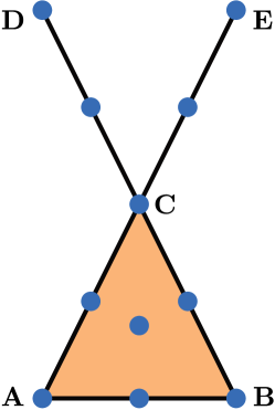
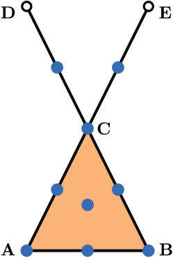
Figure 8. The simplicial complex shown on the left and consisting of the triangle $\mathbf{ABC}$, the edges $\mathbf{AB}$, $\mathbf{AC}$, $\mathbf{BC}$, $\mathbf{CD}$, $\mathbf{CE}$, and the vertices $\mathbf{A}$, $\mathbf{B}$, $\mathbf{C}$, $\mathbf{D}$, and $\mathbf{E}$ is an example of a Lefschetz complex. Simplices are marked with a small circle in the center of mass of each simplex. In the right panel, the simplices marked with a blue circle constitute a locally closed (convex) subset of the set of all simplices. Therefore, it is another example of a Lefschetz complex $X$ which consists of all simplices of the simplicial complex except the vertices $\mathbf{D}$ and $\mathbf{E}$, shown as circles with white interiors.

Example 3.17.

The easiest way to visualize a Lefschetz complex is by presenting it as a $\kappa$-subcomplex of a simplicial complex. A sample Lefschetz complex is presented in Figure 8 as a locally closed collection of simplices of a simplicial complex. Note, however, that not all Lefschetz complexes can be written in this form. $\Diamond$

A Lefschetz subcomplex $A$ of a Lefschetz complex $X$ has its own Lefschetz topology as well as the associated chain complex $C(A)$. As a topological space $A$ is always a subspace of $X$, but $C(A)$ typically is not a chain subcomplex of $X$ unless $A$ is closed in $X$ (see [27, Theorem 5.4]), as the following result shows.

Proposition 3.18.

If $A$ is closed in $X$ in the Lefschetz topology, then

(17) $${\bf\partial}^{\kappa_{|A\times A}}={\bf\partial}^{\kappa}_{|C(A)}$$

and

(18) $${\bf\partial}^{\kappa}(C(A))\subset C(A).$$

In particular, the chain complex $(C(A),{\bf\partial}^{\kappa_{|A\times A}})$ is a chain subcomplex of the chain complex $(C(X),{\bf\partial}^{\kappa})$.

Proof: To see (17) it suffices to verify the equality on basis elements. Thus, take an $x\in A$. Then

$${\bf\partial}^{\kappa_{|A\times A}}x=\sum_{y\in A}\kappa(x,y)y=\sum_{y\in X}\kappa(x,y)y={\bf\partial}^{\kappa}x,$$

because $\kappa(x,y)\neq 0$ implies $y\in\operatorname{cl}x\subset\operatorname{cl}A=A$. Property (18) and the remaining assertion are obvious. ∎

Given a closed subset $A\subset X$ in the Lefschetz topology we define the relative Lefschetz homology $H(X,A)$ as the homology of the quotient chain complex $(C(X,A),\tilde{\partial})$, where $C(X,A):=C(X)/C(A)$ and $\tilde{\partial}$ stands for the induced boundary map. In addition, we also have the following proposition, which follows immediately from [27, Theorem 5.4] (see also [28, Theorem 3.5]), and which uses such a relative homology to characterize the Lefschetz homology of a locally closed $A\subset X$.

Proposition 3.19.

If $A\subset X$ is locally closed in the Lefschetz topology of $X$, then $H(A)$ is isomorphic to the homology $H(\operatorname{cl}A,\operatorname{mo}A)$ of the pair $(\operatorname{cl}A,\operatorname{mo}A)$ of closed subsets of $X$. ∎

The following result was established in [27, Proposition 5.2], and it computes the homology of some simple Lefschetz complexes.

Proposition 3.20.

For every $x\in X$ the singleton $\{x\}$ is a Lefschetz subcomplex of $X$ and

$$H_{q}(\{x\})\cong\begin{cases}R&\text{ if $q=\dim x$,}\\ 0&\text{ otherwise.}\end{cases}$$

For every $x,y\in X$ such that $x$ is a facet of $y$ the doubleton $\{x,y\}$ is a Lefschetz subcomplex of $X$ and for all $q\in\mbox{$\mathbb{Z}$}$ one has

$$H_{q}(\{x,y\})\cong 0.$$

4. Poset filtered chain complexes

In the preliminaries section we recalled basic definitions and properties of chain complexes and their homology. For the definition of the connection matrix, these considerations have to be extended to the case of chain complexes which are poset filtered. In addition, we need to study maps between these poset filtered chain complexes, even in the situation where the filtration posets of the involved chain complexes differ. All of these concepts will be introduced in the current section.

4.1. Graded and filtered module homomorphisms

We begin our discussion on the level of general graded modules. Consider a $K$-graded module $M$ and a $K^{\prime}$-graded module $M^{\prime}$. Let $\alpha:K^{\prime}\nrightarrow K$ be a partial map. We say that a homomorphism $h:M\to M^{\prime}$ is $\alpha$-graded if for every pair of indices $j\in K$ and $i\in K^{\prime}$ we have

$$h_{ij}\neq 0\quad\;\Rightarrow\;\quad i\in\alpha^{-1}(j),$$

which is equivalent to the implication

(19) $$h_{ij}\neq 0\quad\;\Rightarrow\;\quad i\in\operatorname{dom}\alpha\ \ \ \text{and}\ \ \ \alpha(i)=j.$$

If in addition the sets $K$ and $K^{\prime}$ are partially ordered sets and $\alpha$ is order preserving, then we say that a homomorphism $h:M\to M^{\prime}$ is $\alpha$-filtered if for every $j\in K$ and $i\in K^{\prime}$

(20) $$h_{ij}\neq 0\quad\;\Rightarrow\;\quad i\in\alpha^{-1}(j^{\leq})^{\leq}$$

which is equivalent to

$$h_{ij}\neq 0\quad\;\Rightarrow\;\quad\exists_{i^{\prime}\in\operatorname{dom}\alpha}\;i\leq i^{\prime}\ \ \ \text{ and }\ \ \ \alpha(i^{\prime})\leq j.$$

These two definitions are illustrated in Figures 9 and 10. The left image in Figure 9 shows two partially ordered sets together with a partial map $\alpha$ between them. In the right image of the same figure arrows indicate which of the homomorphisms $h_{ij}$ can be nontrivial if $h$ is $\alpha$-graded. In contrast, Figure 10 depicts all possible nontrivial homomorphisms $h_{ij}$ if $h$ is $\alpha$-filtered. The more involved implication (20) is illustrated in the top left image, which indicates the sets $3^{\leq}$ and $b^{\leq}$ in light blue. The remaining three panels in the figure depict all possible nontrivial homomorphisms $h_{ij}$. Clearly, $\alpha$-filtered homomorphisms are far less restricted than $\alpha$-graded ones. In fact, an $\alpha$-filtered homomorphism can have a nontrivial $h_{ij}$ even if $i\not\in\operatorname{dom}\alpha$ or if $j\not\in\operatorname{im}\alpha$.

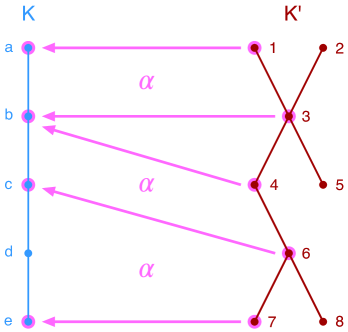
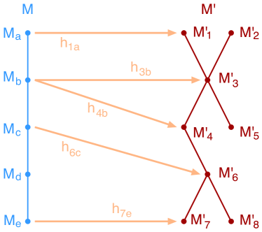
Figure 9. Sample $\alpha$-graded morphism. The left image shows two posets $K$ and $K^{\prime}$, together with an order preserving partial map $\alpha:K^{\prime}\nrightarrow K$. The panel on the right indicates the potential nonzero module homomorphisms $h_{ij}$ if $h$ is $\alpha$-graded.

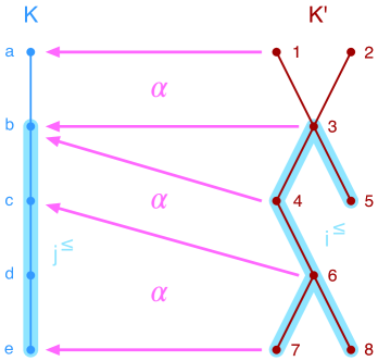
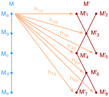
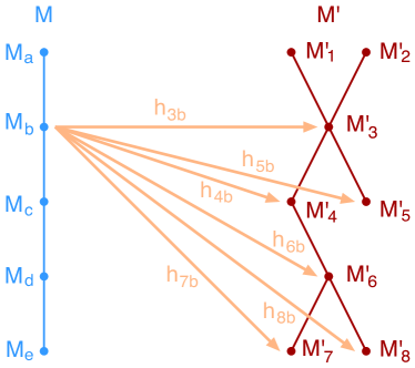
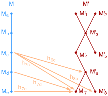
Figure 10. Sample $\alpha$-filtered morphism. The top left image shows two posets $K$ and $K^{\prime}$, together with an order preserving partial map $\alpha:K^{\prime}\nrightarrow K$. The remaining three panels indicate all potentially nonzero module homomorphisms $h_{ij}$ if $h$ is $\alpha$-filtered (top right for $j=a$, bottom left for $j=b$ and bottom right for $j=c,d,e$).

Conditions (19) and (20) for $\alpha$-graded and $\alpha$-filtered homomorphisms, respectively, may be simplified if $\operatorname{dom}\alpha=K^{\prime}$, i.e., if $\alpha$ is actually a function. This is the subject of the following straightforward proposition.

Proposition 4.1.

Assume $\operatorname{dom}\alpha=K^{\prime}$. Then $h:M\to M^{\prime}$ is $\alpha$-graded if and only if for every $i\in K^{\prime}$ and $j\in K$

(21) $$h_{ij}\neq 0\quad\;\Rightarrow\;\quad\alpha(i)=j,$$

and $h$ is $\alpha$-filtered if and only if

(22) $$h_{ij}\neq 0\quad\;\Rightarrow\;\quad\alpha(i)\leq j$$

for every $i\in K^{\prime}$ and $j\in K$. ∎

Obviously, if $\alpha$ is order preserving and $h$ is an $\alpha$-graded homomorphism then $h$ is an $\alpha$-filtered homomorphism. However, the converse is not true in general. This can readily be seen from Figures 9 and 10.

In the case when $K=K^{\prime}$, we say that a homomorphism $h:M\to M^{\prime}$ is $K$-filtered (respectively $K$-graded) if $h$ is $\operatorname{id}_{K}$-filtered (respectively $\operatorname{id}_{K}$-graded). We simplify the terminology to filtered (respectively graded) if $K$ is clear from the context. As an immediate consequence of Proposition 4.1 we get the following corollary.

Corollary 4.2.

An endomorphism $h:M\to M$ on a module $M$ is graded if and only if for every $i,j\in K$ we have

$$h_{ij}\neq 0\quad\;\Rightarrow\;\quad i=j,$$

and $h$ is filtered if and only if one has

$$h_{ij}\neq 0\quad\;\Rightarrow\;\quad i\leq j$$

for every $i,j\in K$. ∎

Note that in the special case when $K=K^{\prime}=\mbox{$\mathbb{Z}$}$ an $\alpha$-graded homomorphism with $\alpha:\mbox{$\mathbb{Z}$}\ni i\mapsto i-k\in\mbox{$\mathbb{Z}$}$ given as the left-shift by $k$ on the integers coincides with a $\mathbb{Z}$-graded homomorphism of degree $k$. We recall that in such a case, when $k$ is clear from the context, we shorten the notation $h_{j+k,j}$ to $h_{j}$.

Proposition 4.3.

Assume that $P$ and $P^{\prime}$ are posets, $\alpha:P^{\prime}\nrightarrow P$ is order preserving, $M$ is a $P$-graded module, and $M^{\prime}$ is a $P^{\prime}$-graded module. A module homomorphism $h:M\to M^{\prime}$ is an $\alpha$-filtered homomorphism if and only if

(23) $$h(M_{L})\subset M^{\prime}_{\alpha^{-1}(L)^{\leq}}$$

for every $L\in\mbox{$\operatorname{Down}$}(P)$.

Proof: Assume that $h:M\to M^{\prime}$ is a module homomorphism such that (23) is satisfied for every $L\in\mbox{$\operatorname{Down}$}(P)$. Moreover, assume that $h_{pq}\neq 0$ for an element $q\in P$ and a $p\in P^{\prime}$. Let $x\in M_{q}$ be such that $h_{pq}(x)\neq 0$. If we consider $L:=q^{\leq}\in\mbox{$\operatorname{Down}$}(P)$, then (23) implies $h(M_{L})\subset M^{\prime}_{\alpha^{-1}(L)^{\leq}}$. Since we have the inclusions $x\in M_{q}\subset M_{L}$, we get $h(x)\in M^{\prime}_{\alpha^{-1}(L)^{\leq}}$. Thus, the identity $h_{p^{\prime}q}(x)=\pi_{p^{\prime}}(h(x))=0$ holds for $p^{\prime}\not\in\alpha^{-1}(L)^{\leq}$, which in turn implies that $p\in\alpha^{-1}(L)^{\leq}$, in view of $h_{pq}(x)=\pi_{p}(h(x))\neq 0$. In consequence, $p\leq\bar{p}$ for a $\bar{p}$ with $\alpha(\bar{p})\in L=q^{\leq}$. Therefore, $p\in\alpha^{-1}(q^{\leq})^{\leq}$ which implies (20) and proves that $h$ is $\alpha$-filtered. To prove the opposite implication, assume that $h:M\to M^{\prime}$ is a module homomorphism such that property (20) holds. Let $L\in\mbox{$\operatorname{Down}$}(P)$ and consider $x\in M_{L}$. Without loss of generality we may assume that $x\in M_{q}$ for a $q\in L$. Then an application of (20) yields

$$h(x)=\sum_{p\in P}h_{pq}(x)=\sum_{p\in\alpha^{-1}(q^{\leq})^{\leq}}h_{pq}(x),$$

which means that $h(x)\in M^{\prime}_{\alpha^{-1}(L)^{\leq}}$, since we have $\alpha^{-1}(q^{\leq})^{\leq}\subset\alpha^{-1}(L)^{\leq}$. This establishes the inclusion in (23). ∎

In the special case when $P=P^{\prime}$ and $\alpha=\operatorname{id}_{P}$ we have the following corollary of Proposition 4.3.

Corollary 4.4.

Assume that $P$ is a poset and that $M$ is a $P$-graded module. Then $h:M\to M$ is a filtered homomorphism if and only if

(24) $$h(M_{L})\subset M_{L}$$

for every $L\in\mbox{$\operatorname{Down}$}(P)$.

Proof: By applying our assumptions $P=P^{\prime}$ and $\alpha=\operatorname{id}_{P}$ to the setting of Proposition 4.3, one obtains that $\alpha^{-1}(L)^{\leq}=L^{\leq}=L$. Therefore, the condition in (23) reduces to the one in (24). ∎

Definition 4.5.

We say that two $P$-gradations $(M_{p})_{p\in P}$ and $(M^{\prime}_{p})_{p\in P}$ of the same module $M$ are filtered equivalent, if for every $L\in\mbox{$\operatorname{Down}$}(P)$ we have $M_{L}=M^{\prime}_{L}$.

As an immediate consequence of Corollary 4.4 one obtains the following proposition.

Proposition 4.6.

Let $P$ be a poset. Assume that $M$ and $M^{\prime}$ are $P$-graded modules and that $h:M\to M^{\prime}$ is a filtered homomorphism. Then $h$ is a filtered homomorphism with respect to any filtered equivalent gradation of the modules $M$ and $M^{\prime}$. ∎

4.2. The category of graded and filtered moduli

We define the two categories GMod of graded moduli and FMod of filtered moduli as follows. The objects of GMod (respectively FMod) are pairs $(P,M)$ where $P$ is an object of DSet (respectively DPSet) and $M$ is a $P$-graded module; (see Section 3.3). The morphisms in GMod (respectively FMod) are pairs $(\alpha,h):(P,M)\to(P^{\prime},M^{\prime})$ such that $\alpha:P^{\prime}\nrightarrow P$ is a morphism in DSet (respectively $\text{\sc DPSet})$ and $h:M\to M^{\prime}$ is an $\alpha$-graded (respectively $\alpha$-filtered) module homomorphism. In the following, we will briefly refer to morphisms in GMod (respectively FMod) as graded (respectively filtered) morphisms $(\alpha,h):(P,M)\to(P^{\prime},M^{\prime})$. In the special case when one has the identities $(P,M)=(P^{\prime},M^{\prime})$ and $\alpha=\operatorname{id}_{P}$ we simplify the terminology by referring to $h$ as a filtered (respectively graded) morphism, meaning that $h$ is $\operatorname{id}_{P}$-filtered (respectively $\operatorname{id}_{P}$-graded).

One can easily verify that $\operatorname{id}_{(P,M)}:=(\operatorname{id}_{P},\operatorname{id}_{M})$ is the identity morphism on $(P,M)$ in both GMod and FMod. Also, if $(\alpha,h):(P,M)\to(P^{\prime},M^{\prime})$ and $(\alpha^{\prime},h^{\prime}):(P^{\prime},M^{\prime})\to(P^{\prime\prime},M^{\prime\prime})$ are two graded or filtered morphisms, then we define their composition

$$(\alpha^{\prime\prime},h^{\prime\prime}):=(\alpha^{\prime},h^{\prime})\circ(\alpha,h):(P,M)\to(P^{\prime\prime},M^{\prime\prime})$$

by $\alpha^{\prime\prime}:=\alpha\alpha^{\prime}$ and $h^{\prime\prime}:=h^{\prime}h$. This leads to the following fundamental results.

Proposition 4.7.

GMod is a well-defined category.

Proof: The only nontrivial part of the proof is the verification that the composition of two graded morphisms is again a graded morphism. For this, let $(\alpha^{\prime\prime},h^{\prime\prime}):=(\alpha^{\prime},h^{\prime})\circ(\alpha,h)$ be given as above. Obviously $h^{\prime}h$ is a module homomorphism. We will show that $h^{\prime\prime}_{pr}\neq 0$ for $p\in P^{\prime\prime}$ and $r\in P$ implies the equality $(\alpha\alpha^{\prime})(p)=r$. Hence, we assume that $h^{\prime\prime}_{pr}\neq 0$ for some $p\in P^{\prime\prime}$ and $r\in P$. It follows from Proposition 3.5 that there exists a $q\in P^{\prime}$ such that both $h^{\prime}_{pq}\neq 0$ and $h_{qr}\neq 0$ are satisfied. This further shows that one has to have $p\in\operatorname{dom}\alpha^{\prime}$ and $\alpha^{\prime}(p)=q$, as well as $q\in\operatorname{dom}\alpha$ and $\alpha(q)=r$. It follows that $p\in\operatorname{dom}(\alpha\alpha^{\prime})$ and $(\alpha\alpha^{\prime})(p)=r$. This proves that $(\alpha^{\prime\prime},h^{\prime\prime})$ is a graded morphism. ∎

A given pair of poset graded morphisms $f:(P,M)\to(P,M)$ and $f^{\prime}:(P^{\prime},M^{\prime})\to(P^{\prime},M^{\prime})$ are called graded-conjugate, if there exists a poset graded isomorphism $(\alpha,h):(P,M)\to(P^{\prime},M^{\prime})$ such that

$$(\alpha,h)\circ f=f^{\prime}\circ(\alpha,h).$$

If the morphisms $f$ and $f^{\prime}$ are graded-conjugate, then we say that their respective $(P,P)$- and $(P^{\prime},P^{\prime})$-matrices are graded-similar. It is easily seen that the graded similarity of matrices is an equivalence relation.

Proposition 4.8.

FMod is a well-defined category.

Proof: The only nontrivial property to verify is that the composition of filtered morphisms is again a filtered morphism. For this, consider a composition $(\alpha^{\prime\prime},h^{\prime\prime}):=(\alpha^{\prime},h^{\prime})\circ(\alpha,h)$ of filtered morphisms as above. Obviously, the map $\alpha\alpha^{\prime}$ is order preserving and $h^{\prime}h$ is a module homomorphism. Thus, we only need to verify that that $h^{\prime\prime}_{pr}\neq 0$ for $p\in P^{\prime\prime}$ and $r\in P$ implies the inclusion $p\in(\alpha\alpha^{\prime})^{-1}(r^{\leq})^{\leq}$. Hence, assume that $h^{\prime\prime}_{pr}\neq 0$ for $p\in P^{\prime\prime}$ and $r\in P$. It follows from Proposition 3.5 that there exists a $q\in P^{\prime}$ such that $h^{\prime}_{pq}\neq 0$ and $h_{qr}\neq 0$. Therefore, there exist $\bar{p}\geq p$ and $\bar{q}\geq q$ such that $\alpha^{\prime}(\bar{p})\leq q$ and $\alpha(\bar{q})\leq r$. Since $\alpha$ is order preserving, it follows that $(\alpha\alpha^{\prime})(\bar{p})\leq\alpha(\bar{q})\leq r$. Hence, $\bar{p}\in(\alpha\alpha^{\prime})^{-1}(r^{\leq})$ and $p\in(\alpha\alpha^{\prime})^{-1}(r^{\leq})^{\leq}$. This proves that $(\alpha^{\prime},h^{\prime\prime})$ is a filtered morphism. ∎

Proposition 4.9.

Assume that the two maps $(\alpha,h):(P,M)\to(P^{\prime},M^{\prime})$ and $(\alpha^{\prime},h^{\prime}):(P^{\prime},M^{\prime})\to(P^{\prime\prime},M^{\prime\prime})$ are morphisms in FMod which satisfy the identities $\operatorname{dom}\alpha=P^{\prime}$ and $\operatorname{dom}\alpha^{\prime}=P^{\prime\prime}$. Suppose further that $\alpha$ is injective. If $p\in P$ and $p^{\prime\prime}\in P^{\prime\prime}$ are such that $\alpha\alpha^{\prime}(p^{\prime\prime})=p$, then

(25) $$(h^{\prime}h)_{p^{\prime\prime}p}=h^{\prime}_{p^{\prime\prime}\alpha^{\prime}(p^{\prime\prime})}h_{\alpha^{\prime}(p^{\prime\prime})p}\quad\text{for $p\in P$.}$$

Proof: We get from Proposition 3.5 that

(26) $$(h^{\prime}h)_{p^{\prime\prime}p}=\sum_{p^{\prime}\in P^{\prime}}{h^{\prime}}_{p^{\prime\prime}p^{\prime}}h_{p^{\prime}p}.$$

It follows from (22) that the index $p^{\prime}$ of a non-zero term on the right-hand side of (26) must satisfy $\alpha^{\prime}(p^{\prime\prime})\leq p^{\prime}$ and $\alpha(p^{\prime})\leq p$. Hence,

$$p=\alpha\alpha^{\prime}(p^{\prime\prime})\leq\alpha(p^{\prime})\leq p.$$

It follows that $\alpha(p^{\prime})=p$ and, since $\alpha$ is injective, we get $p^{\prime}=\alpha^{\prime}(p^{\prime\prime})$. This proves (25). ∎

As an immediate consequence of Proposition 4.9 one obtains the following corollary.

Corollary 4.10.

Assume that the two maps $(\alpha,h):(P,M)\to(P^{\prime},M^{\prime})$ and $(\alpha^{\prime},h^{\prime}):(P^{\prime},M^{\prime})\to(P,M)$ are morphisms in FMod such that $\alpha:P^{\prime}\to P$ and $\alpha^{\prime}:P\to P^{\prime}$ are mutually inverse bijections. Then

$$(h^{\prime}h)_{pp}=h^{\prime}_{p\alpha^{\prime}(p)}h_{\alpha^{\prime}(p)p}\quad\text{for $p\in P$.}$$

Lemma 4.11.

A filtered morphism $(\alpha,h):(P,M)\to(P^{\prime},M^{\prime})$ is an isomorphism in FMod if and only if the map $\alpha:P^{\prime}\to P$ is an order isomorphism and $h_{p^{\prime}\alpha(p^{\prime})}:M_{\alpha(p^{\prime})}\to M^{\prime}_{p^{\prime}}$ is a module isomorphism for every $p^{\prime}\in P^{\prime}$.

Proof: First assume that $(\alpha,h)$ is an isomorphism in the category FMod. Let $(\alpha^{\prime},h^{\prime}):(P^{\prime},M^{\prime})\to(P,M)$ be the inverse of $(\alpha,h)$. Then $\alpha\alpha^{\prime}=\operatorname{id}_{P}$ and $\alpha^{\prime}\alpha=\operatorname{id}_{P^{\prime}}$. Since $\alpha$ and $\alpha^{\prime}$ are order preserving, we see that $\alpha:P^{\prime}\to P$ is an order isomorphism. It follows from Corollary 4.10 that

(27) $$\operatorname{id}_{M_{p}}=(\operatorname{id}_{M})_{pp}=(h^{\prime}h)_{pp}=h^{\prime}_{p\alpha^{\prime}(p)}h_{\alpha^{\prime}(p)p}\text{ for $p\in P$}$$

and

(28) $$\operatorname{id}_{M_{p^{\prime}}}=(\operatorname{id}_{M})_{p^{\prime}p^{\prime}}=(hh^{\prime})_{p^{\prime}p^{\prime}}=h_{p^{\prime}\alpha(p^{\prime})}h^{\prime}_{\alpha(p^{\prime})p^{\prime}}\text{ for $p^{\prime}\in P^{\prime}$.}$$

But, $\alpha$ and $\alpha^{\prime}$ are mutually inverse bijections. Hence, substituting $p^{\prime}:=\alpha^{\prime}(p)$ in (27) we get $p=\alpha(p^{\prime})$ and

$$\operatorname{id}_{M_{\alpha(p^{\prime})}}=h^{\prime}_{\alpha(p^{\prime})p^{\prime}}h_{p^{\prime}\alpha(p^{\prime})}\text{ for $p^{\prime}\in P^{\prime}$.}$$

It follows that $h^{\prime}_{\alpha(p^{\prime})p^{\prime}}$ is the inverse of $h_{p^{\prime}\alpha(p^{\prime})}$. Therefore, $h_{p^{\prime}\alpha(p^{\prime})}$ is a module isomorphism for every $p^{\prime}\in P^{\prime}$.

To see the opposite implication, assume that $(\alpha,h):(P,M)\to(P^{\prime},M^{\prime})$ is a filtered homomorphism such that $\alpha:P^{\prime}\to P$ is an order isomorphism and $h_{p^{\prime}\alpha(p^{\prime})}:M_{\alpha(p^{\prime})}\to M^{\prime}_{p^{\prime}}$ is a module isomorphism for all $p^{\prime}\in P^{\prime}$. Since $P$ and $P^{\prime}$ as objects of DPSet are finite sets, we may proceed by induction on their cardinality $n:=\operatorname{card}P=\operatorname{card}P^{\prime}$. If $n=1$, then $P=\{p\}$, $P^{\prime}=\{p^{\prime}\}$ and $h_{p^{\prime}\alpha(p^{\prime})}=h_{p^{\prime}p}=h$ is a module isomorphism. Clearly, its inverse is a filtered homomorphism. Hence, $h$ is an isomorphism in FMod. Thus, we now assume $n>1$. Let $\bar{p}^{\prime}$ be a maximal element in $P^{\prime}$. Set $\bar{p}:=\alpha(\bar{p}^{\prime})$. Since $\alpha^{\prime}$ is an order isomorphism, we see that $\bar{p}$ is a maximal element in $P$. Let $\bar{P}^{\prime}:=P^{\prime}\setminus\{\bar{p}^{\prime}\}$, $\bar{P}:=P\setminus\{\bar{p}\}$, $\bar{M}^{\prime}:=M_{\bar{P}^{\prime}}$, $\bar{M}:=M_{\bar{P}}$. Let $Q:=\{\bar{P},\bar{p}\}$ and $Q^{\prime}:=\{\bar{P}^{\prime},\bar{p}^{\prime}\}$ be linearly ordered respectively by $\bar{P}<\bar{p}$ and $\bar{P}^{\prime}<\bar{p}^{\prime}$. Then $(Q,M)$ and $(Q^{\prime},M^{\prime})$ are graded modules. Define $\bar{\alpha}:Q^{\prime}\to Q$ through the identities $\bar{\alpha}(\bar{P}^{\prime}):=\bar{P}$ and $\bar{\alpha}(\bar{p}^{\prime}):=\bar{p}$. We will prove that

(29) $$h_{\bar{p}^{\prime}p}=0\text{ for $p\in\bar{P}.$}$$

Arguing by contradiction, assume that $h_{\bar{p}^{\prime}p}\neq 0$ for a $p\in\bar{P}$. Since $h$ is an $\alpha$-filtered homomorphism, we get from (20) that $h_{\bar{p}^{\prime}p}\neq 0$ implies $\bar{p}^{\prime}\leq\bar{\bar{p}}^{\prime}$ for some $\bar{\bar{p}}^{\prime}\in\operatorname{dom}\alpha$ such that $\alpha(\bar{\bar{p}}^{\prime})\leq p$. Since $\bar{p}^{\prime}$ is maximal in $P^{\prime}$, we obtain both $\bar{p}^{\prime}=\bar{\bar{p}}^{\prime}$ and $\bar{p}=\alpha(\bar{p}^{\prime})\leq p$. Since $\bar{p}$ is maximal in $P$, this further implies the equality $p=\bar{p}$, a contradiction proving (29). Hence, the identity in (11) yields $h_{\bar{p}^{\prime}\bar{P}}=\sum_{p\in\bar{P}}h_{\bar{p}^{\prime}p}\circ\pi_{p}=0$. Therefore, the $(Q,Q^{\prime})$-matrix of $h$ is

$$\left[\begin{array}[]{cc}h_{\bar{P}^{\prime}\bar{P}}&h_{\bar{P}^{\prime}\bar{p}}\\ 0&h_{\bar{p}^{\prime}\bar{p}}\end{array}\right].$$

By induction assumption $(\alpha_{|\bar{P}^{\prime}},h_{\bar{P}^{\prime}\bar{P}}):M_{\bar{P}}\to M_{\bar{P}^{\prime}}$ is an isomorphism in FMod. Set $\alpha^{\prime}:=\alpha^{-1}$ and let $h^{\prime}:M^{\prime}\to M$ be the homomorphism given by the $(Q^{\prime},Q)$-matrix

$$\left[\begin{array}[]{cc}h_{\bar{P}^{\prime}\bar{P}}^{-1}&-h_{\bar{P}^{\prime}\bar{P}}^{-1}h_{\bar{P}^{\prime}\bar{p}}h_{\bar{p}^{\prime}\bar{p}}^{-1}\\ 0&h_{\bar{p}^{\prime}\bar{p}}^{-1}\end{array}\right].$$

One easily verifies that $h^{\prime}$ is $\alpha^{\prime}$-filtered and a straightforward computation shows that $(\alpha^{\prime},h^{\prime})\circ(\alpha,h)=\operatorname{id}_{(P,M)}$ and $(\alpha,h)\circ(\alpha^{\prime},h^{\prime})=\operatorname{id}_{(P^{\prime},M^{\prime})}$. Hence, the morphism $(\alpha,h)$ is indeed an isomorphism in FMod. ∎

Corollary 4.12.

Assume $(\alpha,h):(P,M)\to(P^{\prime},M^{\prime})$ is both a homomorphism in GMod and an isomorphism in FMod. Then it is automatically an isomorphism in GMod.

Proof: Due to Lemma 4.11 the map $\alpha:P^{\prime}\to P$ is an order isomorphism and $h_{p^{\prime}\alpha(p^{\prime})}:M_{\alpha(p^{\prime})}\to M^{\prime}_{p^{\prime}}$ is a module isomorphism. Let $g:M^{\prime}\to M$ be the $\alpha^{-1}$-graded homomorphism with $(P^{\prime},P)$-matrix given by

$$g_{pp^{\prime}}:=\begin{cases}h_{p^{\prime}\alpha(p^{\prime})}^{-1}&\text{ if $p=\alpha(p^{\prime})$,}\\ 0&\text{ otherwise.}\end{cases}$$

It is straightforward to verify that $(\alpha^{-1},g)$ is the inverse of $(\alpha,h)$ in GMod. Hence, $(\alpha,h)$ is an isomorphism in GMod. ∎

4.3. Poset filtered chain complexes

Let $P$ be an arbitrary finite set and $(C,d)$ a chain complex. We call $(C,d)$ a $P$-graded chain complex, if $C$ is a $P$-graded module in which each $C_{p}\subset C$ is a $\mathbb{Z}$-graded submodule of $C$. Since the chain complex $C$ is $P$-graded, its boundary homomorphism $d$ has a $(P,P)$-matrix. A partial order $\leq$ in $P$ is called $(C,d)$-admissible, or briefly $d$-admissible, if $d$ is a filtered homomorphism with respect to $(P,\leq)$, i.e., if

(30) $$d_{pq}\neq 0\;\Rightarrow\;p\leq q$$

for all $p,q\in P$. Note that a $(C,d)$-admissible partial order on $P$ may not always exist. However, we have the following straightforward proposition and definition.

Proposition and Definition 4.13.

If a given $P$-graded chain complex $(C,d)$ admits a $(C,d)$-admissible partial order on $P$, then the intersection of all such $(C,d)$-admissible partial orders on $P$ is again a $(C,d)$-admissible partial order on $P$. We call it the native partial order of $d$. ∎

Definition 4.14.

We say that the triple $(P,C,d)$ is a poset filtered chain complex if $P$ is a poset, $(C,d)$ is a $P$-graded chain complex and the partial order in $P$ is $d$-admissible.

Note that for a poset filtered chain complex $(P,C,d)$ the module $C$ is not only $P$-graded but also $\mathbb{Z}$-graded where the $n$th summand of the $\mathbb{Z}$-gradation is the direct sum over $p\in P$ of the $n$th summands in the $\mathbb{Z}$-gradation of $C_{p}$.

Example 4.15.

Consider the set of words

$$X:=\mbox{$\{\,\mathbf{A},\mathbf{B},\mathbf{C},\mathbf{AB},\mathbf{AC},\mathbf{BC},\mathbf{CD},\mathbf{CE},\mathbf{ABC}\,\}$}$$

and the free module $C:=\mbox{$\mathbb{Z}$}_{2}\langle X\rangle$ with basis $X$ and coefficients in the field $\mbox{$\mathbb{Z}$}_{2}$. For a word $x\in X$ define its dimension as one less than the number of characters in $x$ and denote the set of words of dimension $i$ by $X_{i}$. Setting

$$C_{i}:=\begin{cases}\mbox{$\mathbb{Z}$}_{2}\langle X_{i}\rangle&\text{ if $X_{i}\neq\varnothing$,}\\ 0&\text{ otherwise.}\end{cases}$$

for $i\in\mbox{$\mathbb{Z}$}$ we obtain a $\mathbb{Z}$-gradation of $C$ given by

(31) $$C=\bigoplus_{i\in\mbox{$\mathbb{Z}$}}C_{i}.$$

Let $P=\{\mathbf{p},\mathbf{q},\mathbf{r},\mathbf{s},\mathbf{t},\mathbf{u}\}$ be a poset with its partial order $\leq$ defined by the Hasse diagram

(32) $$\begin{diagram}.$$

For $p=\mathbf{p},\mathbf{q},\mathbf{r},\mathbf{s},\mathbf{t},\mathbf{u}\in P$ we define $X_{p}$ respectively as

$$\{\mathbf{A}\},\;\{\mathbf{B}\},\;\{\mathbf{AB}\},\;\{\mathbf{CD}\},\;\{\mathbf{CE}\},\;\{\mathbf{C},\mathbf{AC},\mathbf{BC},\mathbf{ABC}\}.$$

Then $\{X_{p}\}_{p\in P}$ is a partition of $X$ which induces a gradation

(33) $$C=\bigoplus_{p\in P}C_{p}$$

with $C_{p}:=\mbox{$\mathbb{Z}$}_{2}\langle X_{p}\rangle$. Consider the homomorphism $d:C\to C$ of degree $-1$ which is defined on the basis $X$ by the matrix

$$\begin{array}[]{c||c|c|c|cccc|c|c|}&\mathbf{A}&\mathbf{B}&\mathbf{AB}&\mathbf{C}&\mathbf{AC}&\mathbf{BC}&\mathbf{ABC}&\mathbf{CD}&\mathbf{CE}\\ \hline\cr\hline\cr\mathbf{A}&&&1&&1&&&&\\ \hline\cr\mathbf{B}&&&1&&&1&&&\\ \hline\cr\mathbf{AB}&&&&&&&1&&\\ \hline\cr\mathbf{C}&&&&&1&1&&1&1\\ \mathbf{AC}&&&&&&&1&&\\ \mathbf{BC}&&&&&&&1&&\\ \mathbf{ABC}&&&&&&&&&\\ \hline\cr\mathbf{CD}&&&&&&&&&\\ \hline\cr\mathbf{CE}&&&&&&&&&\\ \hline\cr\end{array}.$$

One can immediately verify that $d$ is $P$-filtered and $d^{2}=0$. Therefore, the triple $(P,C,d)$ with the $\mathbb{Z}$-gradation (31) and the $P$-gradation (33) is a well-defined poset filtered chain complex. $\Diamond$

We would like to point out that if $J\subset P$, then $(C_{J},d_{JJ})$ does not need to be a chain complex in general. However, we have the following proposition.

Proposition 4.16.

Assume that $J$ is a convex subset of $P$. Then we have:

• $(C_{J},d_{JJ})$ is a chain complex.

• $(C_{J},d_{JJ})$ is chain isomorphic to the quotient complex $(C_{J^{\leq}}/C_{J^{<}},d^{\prime})$, where $d^{\prime}$ denotes the homomorphism induced by $d_{J^{\leq}J^{\leq}}$. Notice that the quotient complex is well-defined since $J^{<}$ is a down set due to the convexity of $J$.

Proof: In order to prove (i) we need to verify that $d_{JJ}^{2}=0$. Assume first that $J$ is a down set. Let $x\in C_{J}$. Then Corollary 4.4 immediately implies that $dx\in C_{J}$. Hence, one obtains both $d_{JJ}x=(\iota_{J}\circ d\circ\pi_{J})(x)=dx$ and $d_{JJ}^{2}x=d_{JJ}dx=d^{2}x=0$, which yields $d_{JJ}^{2}=0$. If $J$ is just convex, we consider the down sets $I:=J^{<}$ and $K:=J^{\leq}$, which clearly satisfy the identity $K=I\cup J$. Since $d$ is a filtered homomorphism, we have $d_{pq}=0$ for $p\in J$ and $q\in I$. Therefore, the matrix of $d_{KK}$ takes the form

$$\left[\begin{array}[]{cc}d_{II}&d_{IJ}\\ 0&d_{JJ}\end{array}\right].$$

Since $K$ is a down set, we already have verified that $d_{KK}^{2}=0$. It follows that

$$0=d_{KK}^{2}=\left[\begin{array}[]{cc}d_{II}^{2}&d_{II}d_{IJ}+d_{IJ}d_{JJ}\\ 0&d_{JJ}^{2}.\end{array}\right]$$

Thus, $d_{JJ}^{2}=0$, which proves (i).

To establish (ii), we consider again the down sets $I:=J^{<}$ and $K:=J^{\leq}$, as well as the homomorphism $\kappa:C_{J}\ni x\mapsto[x]_{I}\in C_{K}/C_{I}$, where $[x]_{I}$ denotes the equivalence class of $x$ in the quotient module $C_{K}/C_{I}$. Let $x\in C_{J}$ and let $\bar{d}_{KK}$ denote the boundary homomorphism induced by $d_{KK}$ on the quotient module $C_{K}/C_{I}$. We then have

$$\bar{d}_{KK}\kappa x=[dx]_{I}=[d_{IJ}x+d_{JJ}x]_{I}=[d_{JJ}x]_{I}=\kappa d_{JJ}x,$$

and this implies that the map $\kappa$ is a chain map. Assume now that $[x]_{I}=0$ for an $x\in C_{J}$. Then $x\in C_{I}\cap C_{J}=\{0\}$, that is, $x=0$. This proves that $\kappa$ is a monomorphism. Finally, given the class $[y]_{I}\in C_{K}/C_{I}$ generated by $y\in C_{K}$, we have $y=y_{I}+y_{J}$ for a $y_{I}\in C_{I}$ and a $y_{J}\in C_{J}$. It follows that $[y]_{I}=[y_{J}]_{I}=\kappa y_{J}$, proving that $\kappa$ is an epimorphism. Hence, $\kappa$ is an isomorphism. ∎

It is straightforward to observe that the chain complex $(C_{J},d_{JJ})$ in Proposition 4.16(i) is in fact $J$-filtered. Therefore, we have the following proposition.

Proposition 4.17.

Given a filtered chain complex $(P,C,d)$ and a convex subset $J\subset P$, the triple $(J,C_{J},d_{JJ})$ is also a filtered chain complex. We call it the filtered chain complex induced by a convex subset. ∎

Since a singleton $\{p\}\subset P$ is always convex, one immediately obtains the following corollary.

Corollary 4.18.

Let $(P,C,d)$ be an arbitrary poset filtered chain complex. Then the pair $(C_{p},d_{pp})$ is a chain complex for every $p\in P$. ∎

Given a poset filtered chain complex $(P,C,d)$ we consider the poset $P$ as an object of DPSet with the distinguished subset $P_{\star}$ satisfying

(34) $$\mbox{$\{\,p\in P\mid\text{ $C_{p}$ is homotopically essential}\,\}$}\subset P_{\star}.$$

The concrete choice of $P_{\star}$ depends on applications. Typically, the simplest choice which gives equality in (34) suffices. In other situations, however, we might take the other extreme case $P_{\star}=P$, and in this case we call the poset filtered chain complex $(P,C,d)$ peeled.

In terms of applications to dynamics, a choice of a larger $P_{\star}$ can mean that some Morse sets may only be known via isolating neighborhoods and potentially may have zero Conley index. Recall that $C_{p}$ is homotopically essential if it is not chain homotopic to the zero chain complex.

We note that in Example 4.15 the chain complex $(C_{p},d_{pp})$ is essential for $p=\mathbf{p},\mathbf{q},\mathbf{r},\mathbf{s},\mathbf{t}$ and inessential for $p=\mathbf{u}$. Therefore, for the poset $P$ in Example 4.15 there are only two possible choices of $P_{\star}$, namely $P_{\star}=\{\mathbf{p},\mathbf{q},\mathbf{r},\mathbf{s},\mathbf{t}\}$ and $P_{\star}=P$.

4.4. The category of filtered and graded chain complexes

As our next step, we study morphisms between poset filtered chain complexes. For this, consider poset filtered chain complexes $(P,C,d)$ and $(P^{\prime},C^{\prime},d^{\prime})$. Then we say that the map $(\alpha,h):(P,C,d)\to(P^{\prime},C^{\prime},d^{\prime})$ is a filtered chain morphism, if $h:(C,d)\to(C^{\prime},d^{\prime})$ is a chain map and $h$ is a $\alpha$-filtered, that is $(\alpha,h):(P,C)\to(P^{\prime},C^{\prime})$ is a morphism in FMod. We say that the map $(\alpha,h)$ is a graded chain morphism if $h:(C,d)\to(C^{\prime},d^{\prime})$ is a chain map and $h$ is a $\alpha$-graded, that is $(\alpha,h):(P,C)\to(P^{\prime},C^{\prime})$ is a morphism in GMod.

We define the category PfCc of poset filtered chain complexes by taking poset filtered chain complexes as objects and filtered chain morphisms as morphisms. One easily verifies that this is indeed a category. We also define the subcategory PgCc of poset graded chain complexes by taking the same objects as in PfCc and graded chain morphisms as morphisms.

Definition 4.19.

Let $(\alpha,\varphi),(\alpha^{\prime},\varphi^{\prime}):(P,C,d)\to(P^{\prime},C^{\prime},d^{\prime})$ denote a pair of filtered chain morphisms, and let $(\gamma,\Gamma):(P,C)\to(P^{\prime},C^{\prime})$ be a filtered module morphism. Then $(\gamma,\Gamma)$ is called an elementary filtered chain homotopy between $(\alpha,\varphi)$ and $(\alpha^{\prime},\varphi^{\prime})$ if the following conditions are satisfied:

• $\Gamma$ is a module homomorphism of degree $+1$ with respect to the $\mathbb{Z}$-gradation of $C$ and $C^{\prime}$,

• $\Gamma$ is a chain homotopy between $\varphi$ and $\varphi^{\prime}$, that is, $\varphi^{\prime}-\varphi=\Gamma d+d^{\prime}\Gamma$,

• we have the equalities $\alpha_{|P^{\prime}_{\star}}=\gamma_{|P^{\prime}_{\star}}=\alpha^{\prime}_{|P^{\prime}_{\star}}$.

We say that two filtered chain morphisms $(\alpha,h)$ and $(\alpha^{\prime},h^{\prime})$ are elementarily filtered chain homotopic, and we write $(\alpha,h)\sim_{e}(\alpha^{\prime},h^{\prime})$, if there exists an elementary filtered chain homotopy between $(\alpha,h)$ and $(\alpha^{\prime},h^{\prime})$. We say that filtered chain morphisms $(\alpha,h)$, $(\alpha^{\prime},h^{\prime})$ are filtered chain homotopic, and we write $(\alpha,h)\sim(\alpha^{\prime},h^{\prime})$, if there exists a sequence

(35) $$(\alpha,h)=(\alpha_{0},h_{0})\;\sim_{e}\;(\alpha_{1},h_{1})\;\sim_{e}\;\ldots\;\sim_{e}\;(\alpha_{n},h_{n})=(\alpha^{\prime},h^{\prime})$$

of filtered chain morphisms such that successive pairs are elementarily filtered chain homotopic.

The following proposition is straightforward.

Proposition 4.20.

The relation $\sim$ in the set of morphisms from $(P,C,d)$ to $(P^{\prime},C^{\prime},d^{\prime})$ in PfCc is an equivalence relation. ∎

In certain situations, a filtered chain homotopy automatically is an elementary filtered chain homotopy. To state this result, recall that a poset filtered chain complex $(P,C,d)$ is peeled if we have $P_{\star}=P$. Then the following holds.

Proposition 4.21.

Assume that the poset filtered chain complex $(P^{\prime},C^{\prime},d^{\prime})$ is peeled. If $(\alpha,h),(\alpha^{\prime},h^{\prime}):(P,C,d)\to(P^{\prime},C^{\prime},d^{\prime})$ are filtered chain homotopic, then $\alpha=\alpha^{\prime}$, the domain of $\alpha=\alpha^{\prime}$ is $P^{\prime}$, and we have in fact that $(\alpha,h)\sim_{e}(\alpha^{\prime},h^{\prime})$.

Proof: Choose $n+1$ filtered morphisms $(\alpha_{i},h_{i}):(P,C,d)\to(P^{\prime},C^{\prime},d^{\prime})$ as in (35) for $i=0,\ldots,n$. Let $(\gamma_{i},\Gamma_{i}):(P,C)\to(P^{\prime},C^{\prime})$ for $i\in\{1,2,\ldots,n\}$ be an elementary filtered chain homotopy between $(\alpha_{i-1},h_{i-1})$ and $(\alpha_{i},h_{i})$. Since $P^{\prime}_{\star}=P^{\prime}$, we have $\alpha_{i-1}=(\alpha_{i-1})_{|P^{\prime}_{\star}}=(\gamma_{i})_{|P^{\prime}_{\star}}=\gamma_{i}$, as well as the identity $\alpha_{i}=(\alpha_{i})_{|P^{\prime}_{\star}}=(\gamma_{i})_{|P^{\prime}_{\star}}=\gamma_{i}$ for $i\in\{1,2,\ldots,n\}$. It follows then that one has $\alpha_{i}=\alpha_{i-1}$ for all $i$, and thus $\alpha=\alpha^{\prime}$. Moreover, we obtain

(36) $$h_{i}-h_{i-1}=d^{\prime}\Gamma_{i}+\Gamma_{i}d$$

for $i\in\{1,2,\ldots,n\}$. Let $\Gamma:=\sum_{i=1}^{n}\Gamma_{i}$. One easily verifies that $\Gamma$ is an $\alpha$-filtered module homomorphism. Summing (36) for $i=1,\ldots,n$ we get

$$h^{\prime}-h=h_{n}-h_{0}=d^{\prime}\Gamma+\Gamma d.$$

Thus, $(\alpha,\Gamma)$ is an elementary filtered chain homotopy between the filtered morphisms $(\alpha,h)$ and $(\alpha^{\prime},h^{\prime})$. ∎

4.5. Homotopy category of filtered chain complexes

We refer to the equivalence classes of $\sim$ as the homotopy equivalence classes. They enable us to introduce the homotopy category of poset filtered chain complexes, denoted by ChPfCc, by taking poset filtered chain complexes as objects, homotopy equivalence classes of filtered chain morphisms in PfCc as morphisms in ChPfCc, and using the formula

(37) $$[(\beta,g)]_{\sim}\circ[(\alpha,h)]_{\sim}:=[(\alpha\circ\beta,g\circ h)]_{\sim}$$

for any two given filtered morphisms $(\alpha,h)\in\text{\sc PfCc}((P,C,d),(P^{\prime},C^{\prime},d^{\prime}))$ and $(\beta,g)\in\text{\sc PfCc}((P^{\prime},C^{\prime},d^{\prime}),(P^{\prime\prime},C^{\prime\prime},d^{\prime\prime}))$ as the definition of composition of morphisms in ChPfCc. Finally, equivalence classes of identities in PfCc are identities in ChPfCc. The following result verifies that these definitions indeed lead to a category.

Proposition 4.22.

Assume that the filtered chain morphisms

$$(\alpha,h),(\alpha^{\prime},h^{\prime}):(P,C,d)\to(P^{\prime},C^{\prime},d^{\prime})$$

and

$$(\beta,g),(\beta^{\prime},g^{\prime}):(P^{\prime},C^{\prime},d^{\prime})\to(P^{\prime\prime},C^{\prime\prime},d^{\prime\prime})$$

are filtered chain homotopic. Then the compositions

$$(\beta,g)\circ(\alpha,h),(\beta^{\prime},g^{\prime})\circ(\alpha^{\prime},h^{\prime}):(P,C,d)\to(P^{\prime\prime},C^{\prime\prime},d^{\prime\prime})$$

are also filtered chain homotopic. In particular, the category ChPfCc is well-defined.

Proof: Assume that $(\alpha,h)\sim(\alpha^{\prime},h^{\prime})$ and $(\beta,g)\sim(\beta^{\prime},g^{\prime})$. Since $\sim$ is an equivalence relation, it suffices to prove that $(\beta,g)\circ(\alpha,h)\sim(\beta,g)\circ(\alpha^{\prime},h^{\prime})$ and $(\beta,g)\circ(\alpha^{\prime},h^{\prime})\sim(\beta^{\prime},g^{\prime})\circ(\alpha^{\prime},h^{\prime})$. For the same reason, we may assume that $(\alpha,h)\sim_{e}(\alpha^{\prime},h^{\prime})$ and $(\beta,g)\sim_{e}(\beta^{\prime},g^{\prime})$. Let $(\gamma,S):(P,C)\to(P^{\prime},C^{\prime})$ be an elementary filtered chain homotopy between $(\alpha,h)$ and $(\alpha^{\prime},h^{\prime})$. Consider the filtered morphism $(\eta,T):=(\beta,g)\circ(\gamma,S):(P,C)\to(P^{\prime\prime},C^{\prime\prime})$. Then $\eta=\gamma\beta$ and $T=gS$. We will prove that $(\eta,T)$ is an elementary filtered chain homotopy between $(\beta,g)\circ(\alpha,h)$ and $(\beta,g)\circ(\alpha^{\prime},h^{\prime})$. For this, we need to verify properties (i)-(iii) of Definition 4.19. Clearly, $T$ is a degree $+1$ $\mathbb{Z}$-graded module homomorphism. Hence, property (i) is satisfied. To see property (ii), observe that

$$gh^{\prime}-gh=g(h^{\prime}-h)=g(d^{\prime}S+Sd)=d^{\prime\prime}gS+gSd=d^{\prime\prime}T+Td.$$

Finally, in view of the inclusion $\beta(P^{\prime\prime}_{\star})\subset P^{\prime}_{\star}$, which is a consequence of the definition of DPSet, one obtains

$$\alpha\beta_{|P^{\prime\prime}_{\star}}=\alpha_{|P^{\prime}_{\star}}\beta_{|P^{\prime\prime}_{\star}}=\gamma_{|P^{\prime}_{\star}}\beta_{|P^{\prime\prime}_{\star}}=\eta_{|P^{\prime\prime}_{\star}}=\gamma_{|P^{\prime}_{\star}}\beta_{|P^{\prime\prime}_{\star}}=\alpha^{\prime}_{|P^{\prime}_{\star}}\beta_{|P^{\prime\prime}_{\star}}=\alpha^{\prime}\beta_{|P^{\prime\prime}_{\star}}.$$

Altogether, we have verified that $(\beta,g)\circ(\alpha,h)\sim_{e}(\beta,g)\circ(\alpha^{\prime},h^{\prime})$, which in turn immediately implies that also $(\beta,g)\circ(\alpha,h)\sim(\beta,g)\circ(\alpha^{\prime},h^{\prime})$. The equivalence $(\beta,g)\circ(\alpha^{\prime},h^{\prime})\sim(\beta^{\prime},g^{\prime})\circ(\alpha^{\prime},h^{\prime})$ can be shown similarly. ∎

After these preparations the following notions are immediate. We say that a filtered chain morphism $(\alpha,h):(P,C,d)\to(P^{\prime},C^{\prime},d^{\prime})$ is a filtered chain equivalence, if its equivalence class $[(\alpha,h)]$ is an isomorphism in ChPfCc. In addition, we call two poset filtered chain complexes $(P,C,d)$ and $(P^{\prime},C^{\prime},d^{\prime})$ filtered chain homotopic, if they are isomorphic in ChPfCc, that is, if there exist two filtered chain morphisms $(\alpha,\varphi):(P,C,d)\to(P^{\prime},C^{\prime},d^{\prime})$ and $(\alpha^{\prime},\varphi^{\prime}):(P^{\prime},C^{\prime},d^{\prime})\to(P,C,d)$ such that $(\alpha^{\prime},\varphi^{\prime})\circ(\alpha,\varphi)$ is filtered chain homotopic to $\operatorname{id}_{(P,C)}$, and $(\alpha,\varphi)\circ(\alpha^{\prime},\varphi^{\prime})$ is filtered chain homotopic to $\operatorname{id}_{(P^{\prime},C^{\prime})}$. In this situation, the filtered chain morphisms $(\alpha,\varphi)$ and $(\alpha^{\prime},\varphi^{\prime})$ are referred to as mutually inverse filtered chain equivalences. If $(\alpha^{\prime},\varphi^{\prime})\circ(\alpha,\varphi)$ is elementarily filtered chain homotopic to $\operatorname{id}_{(P,C)}$, and $(\alpha,\varphi)\circ(\alpha^{\prime},\varphi^{\prime})$ is elementarily filtered chain homotopic to $\operatorname{id}_{(P^{\prime},C^{\prime})}$, we call morphisms $(\alpha,\varphi)$ and $(\alpha^{\prime},\varphi^{\prime})$ mutually inverse elementary filtered chain equivalences.

We finish this section with the following auxiliary proposition.

Proposition 4.23.

Assume that $(P,C,d)$ is a poset filtered chain complex with the $P$-gradation $(C_{p})_{p\in P}$, and let $(W_{p})_{p\in P}$ denote another $P$-gradation of $C$. If $(C_{p})_{p\in P}$ and $(W_{p})_{p\in P}$ are filtered equivalent in the sense of Definition 4.5, then the triple $(P,W,d)$ with $W:=\bigoplus_{p\in P}W_{p}$ and $P$-gradation given by $(W_{p})_{p\in P}$ is also a poset filtered chain complex. Moreover, $(P,W,d)$ and $(P,C,d)$ are isomorphic in PfCc, and therefore also in ChPfCc.

Proof: Note that $W$ and $C$ are in fact the same modules, but the gradations $(W_{p})_{p\in P}$ and $(C_{p})_{p\in P}$ need not be the same. We know that $d$ is a filtered homomorphism with respect to the $(C_{p})_{p\in P}$ gradation of $C$. Since the $(W_{p})_{p\in P}$ gradation of $W=C$ is filtered equivalent to the $(C_{p})_{p\in P}$ gradation, we see from Proposition 4.6 that $d$ is a filtered homomorphism with respect to the $(W_{p})_{p\in P}$ gradation of $C$ as well. Hence, $(P,W,d)$ is a poset filtered chain complex. We will prove that

(38) $$(\operatorname{id}_{P},\operatorname{id}_{C}):(P,C,d)\to(P,W,d)$$

and

(39) $$(\operatorname{id}_{P},\operatorname{id}_{W}):(P,W,d)\to(P,C,d)$$

are mutually inverse isomorphisms in PfCc. Let $p\in P$. Since both $(C_{p})_{p\in P}$ and $(W_{p})_{p\in P}$ are filtered equivalent, using Proposition 4.16(ii) we get

$$C_{p}\cong C_{p^{\leq}}/C_{p^{<}}=W_{p^{\leq}}/W_{p^{<}}\cong W_{p}.$$

Hence, $C_{p}$ is essential if and only if $W_{p}$ is essential, and from this it follows immediately that $W$ satisfies (34), because $C$ satisfies (34).

Since $(C_{p})_{p\in P}$ and $(W_{p})_{p\in P}$ are filtered equivalent, we get from Corollary 4.4 that $(\operatorname{id}_{P},\operatorname{id}_{C}):(P,C)\to(P,W)$ and $(\operatorname{id}_{P},\operatorname{id}_{W}):(P,W)\to(P,C)$ are filtered morphisms. Clearly, both are chain maps. It follows that the morphisms (38) and (39) are well-defined. Since they are also mutually inverse, the conclusion follows. ∎

5. Algebraic connection matrices

After the preparations of the previous section, we are now in a position to introduce our notion of connection matrices in a purely algebraic way. While the definition is modeled on previous work by Robbin and Salamon [35], as well as Harker, Mischaikow, and Spendlove [14], their approach has to be extended to allow for varying underlying posets. For this, we first introduce the notion of reduced filtered chain complexes, before discussing Conley complexes and connection matrices, as well as their existence for arbitrary poset filtered chain complexes. We close the section with a new equivalence relation for Conley complexes, which enables us to precisely formulate the uniqueness question of connection matrices for the first time. Despite being a completely algebraic criterion based on the notion of essentially graded morphisms, it will later allow us to detect underlying bifurcations in combinatorial dynamics.

5.1. Reduced filtered chain complexes

Recall that by Corollary 4.18, every poset filtered chain complex $(P,C,d)$ gives rise to the induced chain complexes $(C_{p},d_{pp})$ for every $p\in P$. The following definition lies at the heart of the notion of Conley complexes.

Definition 5.1.

We say that a poset filtered chain complex $(P,C,d)$ is reduced, if it is peeled, i.e., if we have $P_{\star}=P$, and if the chain complex $(C_{p},d_{pp})$ is boundaryless for all $p\in P$.

Example 5.2.

The filtered chain complex in Example 4.15 is not reduced, because one can check that $d_{p}$ is not boundaryless for $p=\mathbf{u}$. Consider therefore the different set of words

$$X^{\prime}:=\mbox{$\{\,\mathbf{A},\mathbf{B},\mathbf{AB},\mathbf{AD},\mathbf{AE}\,\}$},$$

a subset $P^{\sharp}:=\{\mathbf{p},\mathbf{q},\mathbf{r},\mathbf{s},\mathbf{t}\}$ of $P$ and a poset $\mbox{$\mathbb{P}$}^{\sharp}=(P^{\sharp},\leq^{\sharp})$ with its partial order $\leq^{\sharp}$ defined by the Hasse diagram

(40) $$\begin{diagram}.$$

Notice that the partial order $\leq^{\sharp}$ is just the restriction to $P^{\sharp}$ of the partial order $\leq$ in the poset $P$ defined in Example 4.15. Proceeding as in Example 4.15 we obtain a $\mbox{$\mathbb{P}$}^{\sharp}$-filtered $\mbox{$\mathbb{Z}$}_{2}$-module $(\mbox{$\mathbb{P}$}^{\sharp},C^{\prime},d^{\prime})$ with $C^{\prime}_{p}:=\mbox{$\mathbb{Z}$}_{2}\langle X^{\prime}_{p}\rangle$, where $X^{\prime}_{p}$ for $p=\mathbf{p},\mathbf{q},\mathbf{r},\mathbf{s},\mathbf{t}$ in $P^{\sharp}$ are defined respectively as

$$\{\mathbf{A}\},\{\mathbf{B}\},\{\mathbf{AB}\},\{\mathbf{AD}\},\{\mathbf{AE}\}$$

and the homomorphism $d^{\prime}:C^{\prime}\to C^{\prime}$ is defined on the basis $X^{\prime}$ by the matrix

(41) $$\begin{array}[]{c||c|c|c|c|c|}d^{\prime}&\mathbf{A}&\mathbf{B}&\mathbf{AB}&\mathbf{AD}&\mathbf{AE}\\ \hline\cr\hline\cr\mathbf{A}&&&1&1&1\\ \hline\cr\mathbf{B}&&&1&&\\ \hline\cr\mathbf{AB}&&&&&\\ \hline\cr\mathbf{AD}&&&&&\\ \hline\cr\mathbf{AE}&&&&&\\ \hline\cr\end{array}\;.$$

One can easily check that the partial order $\leq^{\sharp}$ is $d^{\prime}$-admissible. However, it is not the native partial order of $d^{\prime}$. As the reader may verify, the native partial order of $d^{\prime}$ is the partial order $\leq^{\prime}$ given by the Hasse diagram

(42) $$\begin{diagram},$$

which gives a poset $\mbox{$\mathbb{P}$}^{\prime}=(P^{\sharp},\leq^{\prime})$. Replacing the poset $\mbox{$\mathbb{P}$}^{\sharp}$ in $(\mbox{$\mathbb{P}$}^{\sharp},C^{\prime},d^{\prime})$ by $\mbox{$\mathbb{P}$}^{\prime}$, we obtain a $\mbox{$\mathbb{P}$}^{\prime}$-filtered $\mbox{$\mathbb{Z}$}_{2}$-module $(\mbox{$\mathbb{P}$}^{\prime},C^{\prime},d^{\prime})$ which differs from $(\mbox{$\mathbb{P}$}^{\sharp},C^{\prime},d^{\prime})$ only in the $d^{\prime}$-admissible partial order. Nevertheless, it is another object in PfCc. Note that both $(\mbox{$\mathbb{P}$}^{\sharp},C^{\prime},d^{\prime})$ and $(\mbox{$\mathbb{P}$}^{\prime},C^{\prime},d^{\prime})$ are peeled, because it follows from Proposition 3.20 that $C^{\prime}_{p}$ is homotopically essential for $p\in P^{\sharp}$. Therefore, we get from Proposition 4.21 that $(\mbox{$\mathbb{P}$}^{\sharp},C^{\prime},d^{\prime})$ and $(\mbox{$\mathbb{P}$}^{\prime},C^{\prime},d^{\prime})$ are neither isomorphic in PfCc nor in ChPfCc, because otherwise $\mbox{$\mathbb{P}$}^{\sharp}$ and $\mbox{$\mathbb{P}$}^{\prime}$ would be isomorphic as posets. We note that both $(\mbox{$\mathbb{P}$}^{\sharp},C^{\prime},d^{\prime})$ and $(\mbox{$\mathbb{P}$}^{\prime},C^{\prime},d^{\prime})$ are also reduced, because $d^{\prime}_{pp}=0$ for every index $p\in P^{\sharp}$. $\Diamond$

Proposition 5.3.

Assume that $(P,C,d)$ and $(P^{\prime},C^{\prime},d^{\prime})$ are two reduced poset filtered chain complexes and that $(\alpha,h),(\beta,g):(P,C,d)\to(P^{\prime},C^{\prime},d^{\prime})$ are filtered chain homotopic morphisms. If $\alpha$ is injective, then for $p\in P$ and $q\in P^{\prime}$ we have

$$\alpha(q)=p\;\Rightarrow\;h_{qp}=g_{qp}.$$

Proof: Since $(P^{\prime},C^{\prime},d^{\prime})$ is reduced, it is peeled. Thus, we get from Proposition 4.21 that $\alpha=\beta:P^{\prime}\to P$ and there exists an $\alpha$-filtered degree $+1$ homomorphism $\Gamma:C\to C^{\prime}$ such that $g-h=d^{\prime}\Gamma+\Gamma d$. Since $(P,C,d)$ and $(P^{\prime},C^{\prime},d^{\prime})$ are reduced, we get from Proposition 4.9 the identities

$$g_{qp}-h_{qp} = (d^{\prime}\Gamma)_{qp}+(\Gamma d)_{qp}=d^{\prime}_{q\operatorname{id}(q)}\Gamma_{\operatorname{id}(q)p}+\Gamma_{q\alpha(q)}d_{\alpha(q)p}$$

$$= 0\Gamma_{qp}+\Gamma_{qp}0=0.$$

For this, recall also that $d$ and $d^{\prime}$ are $\operatorname{id}_{P}$-filtered, and that $\operatorname{id}_{P}$ is injective. This completes the proof. ∎

If two poset filtered chain complexes $(P,C,d)$ and $(P^{\prime},C^{\prime},d^{\prime})$ are filtered chain homotopic, then the equivalence class of every filtered chain equivalence $(\alpha,\varphi):(P,C,d)\to(P^{\prime},C^{\prime},d^{\prime})$ is automatically an isomorphism in ChPfCc. However, in the category PfCc one has to prove that fact. This is addressed in the following result.

Theorem 5.4.

Assume that the two poset filtered chain complexes $(P,C,d)$ and $(P^{\prime},C^{\prime},d^{\prime})$ are reduced. If they are filtered chain homotopic, then every filtered chain equivalence $(\alpha,\varphi):(P,C,d)\to(P^{\prime},C^{\prime},d^{\prime})$ is an isomorphism in PfCc. In particular, $(P,C,d)$ and $(P^{\prime},C^{\prime},d^{\prime})$ are isomorphic in PfCc.

Proof: Assume that both $(P,C,d)$ and $(P^{\prime},C^{\prime},d^{\prime})$ are reduced. Then we have $P_{\star}=P$ and $P^{\prime}_{\star}=P^{\prime}$. Let $(\alpha^{\prime},\varphi^{\prime}):(P^{\prime},C^{\prime},d^{\prime})\to(P,C,d)$ be a filtered chain morphism such that one has both $(\alpha^{\prime},\varphi^{\prime})\circ(\alpha,\varphi)\sim\operatorname{id}_{(P,C,d)}$ and $(\alpha,\varphi)\circ(\alpha^{\prime},\varphi^{\prime})\sim\operatorname{id}_{(P^{\prime},C^{\prime},d^{\prime})}$. Clearly, $\operatorname{id}_{P}$ and $\operatorname{id}_{P^{\prime}}$ are injective. Hence, it follows from Proposition 5.3 that

$$(\varphi^{\prime}\varphi)_{pp}=(\operatorname{id}_{C})_{pp}=\operatorname{id}_{C_{p}}\quad\text{ and }\quad(\varphi\varphi^{\prime})_{qq}=(\operatorname{id}_{C^{\prime}})_{qq}=\operatorname{id}_{C^{\prime}_{q}}$$

for arbitrary $p\in P$ and $q\in P^{\prime}$. Therefore, it follows from Corollary 4.10 that $(\operatorname{id}_{C})_{pp}=\varphi^{\prime}_{p\alpha^{\prime}(p)}\varphi_{\alpha^{\prime}(p)p}$ for $p\in P$. Similarly we obtain the identity $(\operatorname{id}_{C^{\prime}})_{p^{\prime}p^{\prime}}=\varphi_{p^{\prime}\alpha(p^{\prime})}\varphi^{\prime}_{\alpha(p^{\prime})p^{\prime}}$ for $p^{\prime}\in P^{\prime}$. Since $\alpha$, $\alpha^{\prime}$ are mutually inverse bijections, we may substitute $\alpha^{\prime}(p)$ for $p^{\prime}$ and we get $(\operatorname{id}_{C^{\prime}})_{\alpha^{\prime}(p)\alpha^{\prime}(p)}=\varphi_{\alpha^{\prime}(p)p}\varphi^{\prime}_{p\alpha^{\prime}(p)}$ Hence, we conclude that $\varphi_{\alpha^{\prime}(p)p}$ and $\varphi^{\prime}_{p\alpha^{\prime}(p)}$ are mutually inverse module homomorphisms. Thus, it follows from Lemma 4.11 that $(\alpha,\varphi)$ is an isomorphism in FMod. Since $\varphi$ is a chain map, by Proposition 3.6 its inverse is also a chain map. Hence, $(\alpha,\varphi)$ is an isomorphism in PfCc, which proves that $(P,C,d)$ and $(P^{\prime},C^{\prime},d^{\prime})$ are isomorphic in PfCc. ∎

5.2. Conley complexes and connection matrices

We now turn our attention the the definition of the Conley complex and the associated connection matrix. For this, we need two additional concepts.

Definition 5.5.

Let $(P,C,d)$ be a given poset filtered chain complex. By a representation of $(P,C,d)$ we mean a triple $((P^{\prime},C^{\prime},d^{\prime}),(\alpha,\varphi),(\beta,\psi))$ such that $(P^{\prime},C^{\prime},d^{\prime})$ is an object in PfCc and $(\alpha,\varphi):(P,C,d)\to(P^{\prime},C^{\prime},d^{\prime})$, $(\beta,\psi):(P^{\prime},C^{\prime},d^{\prime})\to(P,C,d)$ are mutually inverse elementary chain equivalences such that $\alpha$ and $\beta$ are strict, that is, $\operatorname{dom}\alpha=P^{\prime}_{\star}$ and $\operatorname{dom}\beta=P_{\star}$. To simplify the terminology, in the sequel we refer to the object $(P^{\prime},C^{\prime},d^{\prime})$ as a representation of $(P,C,d)$, assuming that the associated mutually inverse elementary chain equivalences $(\alpha,\varphi)$ and $(\beta,\psi)$ are implicitly given.

Proposition 5.6.

Given a representation $((P^{\prime},C^{\prime},d^{\prime}),(\alpha,\varphi),(\beta,\psi))$ of $(P,C,d)$, the maps $\alpha:P^{\prime}_{\star}\to P_{\star}$ and $\beta:P_{\star}\to P^{\prime}_{\star}$ are mutually inverse order preserving bijections.

Proof: Since $\alpha$ and $\beta$ are strict, we get from the definition of elementary chain homotopy

$$\operatorname{id}_{P_{\star}} =(\alpha\beta)_{P_{\star}}=\alpha_{P^{\prime}_{\star}}\beta_{P_{\star}}=\alpha\beta,$$

$$\operatorname{id}_{P^{\prime}_{\star}} =(\beta\alpha)_{P^{\prime}_{\star}}=\beta_{P_{\star}}\alpha_{P^{\prime}_{\star}}=\beta\alpha.$$

∎

Let $((P^{\prime},C^{\prime},d^{\prime}),(\alpha,\varphi),(\beta,\psi))$ and $((P^{\prime\prime},C^{\prime\prime},d^{\prime\prime}),(\alpha^{\prime},\varphi^{\prime}),(\beta^{\prime},\psi^{\prime}))$ be two representations of a filtered chain complex $(P,C,d)$.

Definition 5.7.

We define the transfer morphism from the filtered chain complex $(P^{\prime},C^{\prime},d^{\prime})$ to the filtered chain complex $(P^{\prime\prime},C^{\prime\prime},d^{\prime\prime})$ as the filtered chain morphism $(\beta\alpha^{\prime},\varphi^{\prime}\psi)$.

Note that the pair of transfer morphisms $(\beta\alpha^{\prime},\varphi^{\prime}\psi)$ from $(P^{\prime},C^{\prime},d^{\prime})$ to $(P^{\prime\prime},C^{\prime\prime},d^{\prime\prime})$ and $(\beta^{\prime}\alpha,\varphi\psi^{\prime})$ from $(P^{\prime\prime},C^{\prime\prime},d^{\prime\prime})$ to $(P^{\prime},C^{\prime},d^{\prime})$ are mutually inverse chain equivalences.

After these preparations we can now define the central concept of this paper. For this, let $(P,C,d)$ denote an arbitrary poset filtered chain complex. Then the following definition builds upon Definitions 5.1 and 5.5 and introduces both the notions of Conley complex and of connection matrix.

Definition 5.8.

By a Conley complex of $(P,C,d)$ we mean every reduced representation $(\bar{P},\bar{C},\bar{d})$ of $(P,C,d)$. The $(\bar{P},\bar{P})$-matrix of the boundary homomorphism $\bar{d}$ is then called a connection matrix of the poset filtered chain complex $(P,C,d)$.

Since a Conley complex $(\bar{P},\bar{C},\bar{d})$ of a filtered chain complex $(P,C,d)$ is reduced, we have $\bar{P}_{\star}=\bar{P}$ and, in view of Proposition 5.6, we see that $\bar{P}$ is order isomorphic to $P_{\star}$. Therefore, in a Conley complex $(\bar{P},\bar{C},\bar{d})$ of $(P,C,d)$ we can identify the poset $\bar{P}$ with $P_{\star}$, the map $\alpha$ with the inclusion map $\iota_{P}:P_{\star}\hookrightarrow P$, and the map $\beta$ with $\iota_{P}^{-1}:P\nrightarrow P_{\star}$. We do so in the sequel. Clearly, the Conley complex $(\bar{P},\bar{C},\bar{d})$ is chain homotopic to $(P,C,d)$. Therefore, we have the following straightforward proposition.

Proposition 5.9.

If $(P_{\star},\bar{C},\bar{d})$ is a Conley complex of a filtered chain complex $(P,C,d)$, then $H(\bar{C},\bar{d})$ is isomorphic to $H(C,d)$. ∎

As an immediate consequence of Theorem 5.4, we obtain the following two corollaries, which show that these notions are well-defined.

Corollary 5.10.

The Conley complex of a poset filtered chain complex is unique up to an isomorphism in PfCc. In particular, the transfer homomorphism between two Conley complexes of a given poset filtered chain complex is an isomorphism in PfCc. ∎

Corollary 5.11.

If two poset filtered chain complexes are filtered chain homotopic, that is, isomorphic in ChPfCc, then their Conley complexes are isomorphic in PfCc. ∎

Example 5.12.

One can verify that the reduced filtered chain complex $(\mbox{$\mathbb{P}$}^{\sharp},C^{\prime},d^{\prime})$ in Example 5.2 with poset $\mbox{$\mathbb{P}$}^{\sharp}=(P^{\sharp},\leq^{\sharp})$ and $\leq^{\sharp}$ given by the Hasse diagram (40) is a Conley complex of the filtered chain complex in Example 4.15 with the associated connection matrix (41). More precisely, consider the inclusion map $\varepsilon:P^{\sharp}\ni x\mapsto x\in P$ and homomorphisms $h^{\prime}:C\to C^{\prime}$ and $g^{\prime}:C^{\prime}\to C$ given by the matrices

$$\begin{array}[]{c||c|c|c|cccc|c|c|}h^{\prime}&\mathbf{A}&\mathbf{B}&\mathbf{AB}&\mathbf{C}&\mathbf{AC}&\mathbf{BC}&\mathbf{ABC}&\mathbf{CD}&\mathbf{CE}\\ \hline\cr\hline\cr\mathbf{A}&1&&&1&&&&&\\ \hline\cr\mathbf{B}&&1&&&&&&&\\ \hline\cr\mathbf{AB}&&&1&&&1&&&\\ \hline\cr\mathbf{AD}&&&&&&&&1&\\ \hline\cr\mathbf{AE}&&&&&&&&&1\\ \hline\cr\end{array}$$

and

$$\begin{array}[]{c||c|c|c|c|c|}g^{\prime}&\mathbf{A}&\mathbf{B}&\mathbf{AB}&\mathbf{AD}&\mathbf{AE}\\ \hline\cr\hline\cr\mathbf{A}&1&&&&\\ \hline\cr\mathbf{B}&&1&&&\\ \hline\cr\mathbf{AB}&&&1&&\\ \hline\cr\mathbf{C}&&&&&\\ \mathbf{AC}&&&&1&1\\ \mathbf{BC}&&&&&\\ \mathbf{ABC}&&&&&\\ \hline\cr\mathbf{CD}&&&&1&\\ \hline\cr\mathbf{CE}&&&&&1\\ \hline\cr\end{array}.$$

One can verify that

$$(\varepsilon,h^{\prime}):(P,C,d)\to(\mbox{$\mathbb{P}$}^{\sharp},C^{\prime},d^{\prime})\text{ and }(\varepsilon^{-1},g^{\prime}):(\mbox{$\mathbb{P}$}^{\sharp},C^{\prime},d^{\prime})\to(P,C,d),$$

with the partial map $\varepsilon^{-1}:P\nrightarrow P^{\sharp}$ defined as the inverse relation of $\varepsilon$, are mutually inverse elementary filtered chain equivalences. This implies that a Conley complex of the filtered chain complex $(P,C,d)$ in Example 4.15 is given by the representation $((\mbox{$\mathbb{P}$}^{\sharp},C^{\prime},d^{\prime}),(\varepsilon,h^{\prime}),(\varepsilon^{-1},g^{\prime}))$. $\Diamond$

5.3. Existence of Conley complexes

We now turn our attention to the question of existence, i.e., does every poset filtered chain complex have an associated Conley complex and connection matrix? Although in our setting the poset in a poset filtered chain complex is not fixed as in [14, 35], the existence proof of a Conley complex for a poset filtered chain complex in our sense can be adapted from the argument in [35, Theorem 8.1, Corollary 8.2]. For the sake of completeness, we present the details. We begin with a technical lemma, which is a counterpart to [35, Theorem 8.1].

Lemma 5.13.

Assume that $P\neq\varnothing$ and that $(P,C,d)$ denotes an arbitrary poset filtered chain complex with field coefficients. Then there exist four families $\{W_{p}\}_{p\in P}$, $\{V_{p}\}_{p\in P}$, $\{B_{p}\}_{p\in P}$, $\{H_{p}\}_{p\in P}$ of $\mathbb{Z}$-graded submodules of $C$ such that the following statements are satisfied:

• The family $\{W_{p}\}_{p\in P}$ is a $P$-gradation of $C$ which is filtered equivalent to the gradation $\{C_{p}\}_{p\in P}$. In particular, $C=\bigoplus_{p\in P}W_{p}$.

• For every $p\in P$ we have $W_{p}=V_{p}\oplus H_{p}\oplus B_{p}$.

• The inclusion $d(V_{p})\subset B_{p}$ holds, and $d_{|V_{p}}:V_{p}\to B_{p}$ is a module isomorphism, for every $p\in P$.

• The identity $d_{pp}(H_{p})=0$ is satisfied for all $p\in P$.

• For $H:=\bigoplus_{p\in P}H_{p}$ we have $d(H)\subset H$ and $(P,H,d_{|H})$ is a poset filtered chain complex.

Proof: Assume that $(P,C,d)$ is a poset filtered chain complex. We proceed by induction on $n:=\operatorname{card}P$. First assume that $n=1$. Let $p_{*}$ be the unique element of $P$. Then $C=C_{p_{*}}$. We set $W_{p_{*}}:=C$. It follows that the $P$-gradations $(C_{p})_{p\in P}$ and $(W_{p})_{p\in P}$ are identical, and therefore they are filtered equivalent, i.e., (i) is satisfied. The existence of $V_{p_{*}}$, $B_{p_{*}}$, $H_{p_{*}}$ satisfying properties (ii)-(v) then follows from Proposition 3.10.

Now assume that $n>1$. Let $r\in P$ be a maximal element in $P$ and consider the down set $P^{\prime}:=P\setminus\{r\}\in\mbox{$\operatorname{Down}$}(P)$. Let $C^{\prime}:=\bigoplus_{p\in P^{\prime}}C_{p}$. Since $d$ is a filtered homomorphism, we have $d(C^{\prime})\subset C^{\prime}$. Thus, $(P^{\prime},C^{\prime},d_{|C^{\prime}})$ is a $P^{\prime}$-filtered chain complex. Since $\operatorname{card}P^{\prime}=n-1$, by our induction hypothesis, there exist families $\{W_{p}\}_{p\in P^{\prime}}$, $\{V_{p}\}_{p\in P^{\prime}}$, $\{B_{p}\}_{p\in P^{\prime}}$, $\{H_{p}\}_{p\in P^{\prime}}$ of submodules such that properties (i)-(iv) hold for $(P^{\prime},C^{\prime},d_{|C^{\prime}})$. In order to have respective families for $(P,C,d)$ we will extend the families over $P^{\prime}$ to families over $P$ by constructing in turn the modules $V_{r}$, $B_{r}$, $H_{r}$ and $W_{r}$.

To begin with, for a family $\{M_{p}\}_{p\in P^{\prime}}$ of submodules of $C$ which satisfies the identity $M_{p}\cap M_{q}=\{0\}$ for all $p\neq q$, and an $L\in\mbox{$\operatorname{Down}$}(P^{\prime})$, we recall the notation

$$M_{L}:=\bigoplus_{p\in L}M_{p}.$$

Set $C^{\prime}:=C_{P^{\prime}}$, $W^{\prime}:=W_{P^{\prime}}$, $V^{\prime}:=V_{P^{\prime}}$, $B^{\prime}:=B_{P^{\prime}}$, and $H^{\prime}:=H_{P^{\prime}}$. Then from (i) and (ii) applied to $(P^{\prime},C^{\prime},d_{|C^{\prime}})$ we get

(43) $$C^{\prime}_{L}=C_{L}=W_{L}=V_{L}\oplus H_{L}\oplus B_{L}\quad\text{ for every }\quad L\in\mbox{$\operatorname{Down}$}(P^{\prime}).$$

We will show that

(44) $$V^{\prime}\cap(H^{\prime}+d(C))=0.$$

Indeed, if $x\in V^{\prime}$ and $x=x_{1}+dx_{2}$ for an $x_{1}\in H^{\prime}$ and an $x_{2}\in C$, then one obtains $dx=dx_{1}$. By (v) of the induction assumption, $(P^{\prime},H^{\prime},d_{|H^{\prime}})$ is a poset filtered chain complex. Hence, $dx=dx_{1}=d_{|H^{\prime}}x_{1}\in H^{\prime}$. Also, by (iii) of the induction assumption we have $dx\in B^{\prime}$, and therefore $dx\in H^{\prime}\cap B^{\prime}=0$. Since $x\in V^{\prime}$ one then obtains $x=0$. This proves (44).

Since $d^{-1}(C_{r^{<}})\cap C_{r^{\leq}}$ is a $\mathbb{Z}$-graded submodule of $C_{r^{\leq}}$, we can find a $\mathbb{Z}$-graded submodule $V_{r}$ of $C_{r^{\leq}}$ such that

(45) $$C_{r^{\leq}}=(d^{-1}(C_{r^{<}})\cap C_{r^{\leq}})\oplus V_{r},$$

where we also use the fact that the modules have field coefficients. We will prove that

(46) $$d^{-1}(C_{r^{<}})\cap C_{r^{\leq}}=C_{r^{<}}+(d^{-1}(H_{r^{<}})\cap C_{r^{\leq}}).$$

To see that the right-hand side of (46) is contained in the left-hand side observe that the right-hand side is obviously contained in $C_{r^{\leq}}$. Since $C$ is a filtered chain complex and $r^{<}$ is a down set, we have $d(C_{r^{<}})\subset C_{r^{<}}$ and, in consequence, $C_{r^{<}}\subset d^{-1}(C_{r^{<}})$. We also have $d^{-1}(H_{r^{<}})\subset d^{-1}(C_{r^{<}})$, because $H_{r^{<}}\subset W_{r^{<}}$ by (ii) and $W_{r^{<}}=C_{r^{<}}$ by (i). To prove the opposite inclusion take an $x\in C_{r^{\leq}}\cap d^{-1}(C_{r^{<}})$. Then $dx\in C_{r^{<}}$. Hence, by (43), we can find $x_{V}\in V_{r^{<}}$, $x_{H}\in H_{r^{<}}$ and $x_{B}\in B_{r^{<}}$ such that $dx=x_{V}+x_{H}+x_{B}$. From (iii) we get $x_{B}=dy_{V}$ for some $y_{V}\in V_{r^{<}}$. It follows that $x_{V}=d(x-y_{V})-x_{H}$. Hence, $x_{V}\in V_{r^{<}}\cap(d(C)+H_{r^{<}})\subset V^{\prime}\cap(d(C)+H^{\prime})$. Thus, from (44) we get $x_{V}=0$ and $d(x-y_{V})=x_{H}\in H_{r^{<}}$ which means $x-y_{V}\in d^{-1}(H_{r^{<}})$. We also have $x\in C_{r^{\leq}}$ and $y_{V}\in V_{r^{<}}\subset C_{r^{<}}\subset C_{r^{\leq}}$. Therefore, one finally obtains $x=y_{V}+(x-y_{V})\in C_{r^{<}}+(C_{r^{\leq}}\cap d^{-1}(H_{r^{<}}))$. This completes the proof of (46).

Now set $B_{r}:=d(V_{r})$. We will prove that

(47) $$B_{r}\cap C_{r^{<}}=0.$$

Let $x\in B_{r}\cap C_{r^{<}}$. Then $x=dy$ for some $y\in V_{r}\subset C_{r^{\leq}}$. Since $x\in C_{r^{<}}$, we get $y\in d^{-1}(C_{r^{<}})$. Therefore, $y\in V_{r}\cap C_{r^{\leq}}\cap d^{-1}(C_{r^{<}})$. It follows from (45) that $y=0$. Hence, $x=d0=0$, which proves (47).

Since $(P,C,d)$ is a poset filtered chain complex, the boundary homomorphism $d$ is a filtered homomorphism. Therefore, we have $C_{r^{<}}\subset d^{-1}(C_{r^{<}})$. Obviously, $C_{r^{<}}\subset C_{r^{\leq}}$ and $B_{r}=d(V_{r})\subset d(C_{r^{\leq}})\cap d^{-1}(0)\subset C_{r^{\leq}}\cap d^{-1}(H_{r^{<}})$. Thus, by (47), we have a direct sum of $\mathbb{Z}$-graded submodules

(48) $$(C_{r^{<}}\cap d^{-1}(H_{r^{<}}))\oplus B_{r}\subset C_{r^{\leq}}\cap d^{-1}(H_{r^{<}}).$$

Hence, we can choose a $\mathbb{Z}$-graded submodule $H_{r}$ such that

(49) $$C_{r^{\leq}}\cap d^{-1}(H_{r^{<}})=(C_{r^{<}}\cap d^{-1}(H_{r^{<}}))\oplus B_{r}\oplus H_{r}.$$

Thus, it follows from (46) and Proposition 3.3 that

(50) $$C_{r^{\leq}}\cap d^{-1}(C_{r^{<}})=C_{r^{<}}\oplus B_{r}\oplus H_{r}.$$

Therefore, setting $W_{r}:=V_{r}\oplus B_{r}\oplus H_{r}$ we get from (45) that

(51) $$C_{r^{\leq}}=C_{r^{<}}\oplus W_{r}.$$

We now have well-defined families $\{W_{p}\}_{p\in P}$, $\{V_{p}\}_{p\in P}$, $\{B_{p}\}_{p\in P}$, $\{H_{p}\}_{p\in P}$ of submodules of $C$. We will prove that they indeed satisfy properties (i)-(v) for $(P,C,d)$. To prove (i) observe that by (51)

$$C=C_{P^{\prime}\cup r^{\leq}}=C^{\prime}+C_{r^{\leq}}=C^{\prime}+C_{r^{<}}+W_{r}=C^{\prime}+W_{r}.$$

We claim that $C=C^{\prime}\oplus W_{r}$. Indeed, by (51) we have $W_{r}\subset C_{r^{\leq}}$. Therefore, $W_{r}\cap C^{\prime}\subset W_{r}\cap C_{r^{\leq}}\cap C^{\prime}=W_{r}\cap C_{r^{<}}=0$. This together with the induction assumption shows that

$$C=\bigoplus_{p\in P}W_{p}.$$

To show that $(W_{p})_{p\in P}$ is filtered equivalent to $(C_{p})_{p\in P}$, one needs to verify that $C_{L}=W_{L}$ for all $L\in\mbox{$\operatorname{Down}$}(P)$. Note that by the induction assumption

(52) $$C_{L}=W_{L}\quad\text{ for }\quad L\in\mbox{$\operatorname{Down}$}(P^{\prime}).$$

Thus, we only need to consider the case when $r\in L$. Let $L^{\prime}:=L\setminus\{r\}$. Then $L=L^{\prime}\cup r^{\leq}$, and (52) and (51) yield

$$C_{L}=C_{L^{\prime}}+C_{r^{\leq}}=W_{L^{\prime}}+C_{r^{<}}+W_{r}=W_{L^{\prime}}+W_{r^{<}}+W_{r}=W_{L^{\prime}}+W_{r^{\leq}}=W_{L}.$$

This proves property (i). By the induction assumption properties (ii)-(v) need to be verified only for $p=r$. Property (ii) for $p=r$ follows from the definition of $W_{r}$. To see (iii) for $p=r$ take an $x\in V_{r}$ such that $dx=0\in C_{r^{<}}$. Since the inclusion $V_{r}\subset C_{r^{\leq}}$ holds, it follows that $x\in V_{r}\cap C_{r^{\leq}}\cap d^{-1}(C_{r^{<}})$ and we get from (45) that $x=0$. Thus, $d_{|V_{r}}$ is a monomorphism. By the definition of $B_{r}$ it is an epimorphism, which proves (iii). Finally, by (49) we have $H_{r}\subset d^{-1}(H_{r^{<}})$ which implies

(53) $$d(H_{r})\subset H_{r^{<}}.$$

Therefore, $d_{rr}(H_{r})=0$ which proves (iv) for $p=r$. To show that $(P,H,d_{|H})$ is a poset filtered chain complex, we will prove that

(54) $$d(H_{L})\subset H_{L} L\in\mbox{$\operatorname{Down}$}(P)$$ for every .

Property (54) holds by our induction assumption if one has $r\not\in L$. Thus, assume $r\in L$ and set $L^{\prime}:=L\setminus\{r\}$. Then we have $H_{L}=H_{L^{\prime}}+H_{r^{<}}+H_{r}$, and by (53) and the induction assumption one further obtains

$$d(H_{L})\subset d(H_{L^{\prime}})+d(H_{r^{<}})+d(H_{r})\subset H_{L^{\prime}}+H_{r^{<}}\subset H_{L},$$

which proves (54). Since $P\in\mbox{$\operatorname{Down}$}(P)$ and $H_{P}=H$, we get from (53) that the restriction $d_{|H}:H\to H$ is well-defined. Since $d^{2}=0$ and $d(H)\subset H$, we get $d_{|H}^{2}=0$. This proves that $(H,d_{|H})$ is a chain complex. From (54) and Corollary 4.4 one finally can conclude that $d_{|H}$ is a filtered homomorphism. This proves (v) and completes the proof of the lemma. ∎

After these preparations we can now prove the main result of this section, which guarantees the existence of a Conley complex and associated connection matrix for every poset filtered chain complex.

Theorem 5.14.

Every poset filtered chain complex admits a Conley complex and a connection matrix.

Proof: Assume that $(P,C,d)$ is an arbitrary poset filtered chain complex. Let $\{W_{p}\}_{p\in P}$, $\{V_{p}\}_{p\in P}$, $\{B_{p}\}_{p\in P}$, $\{H_{p}\}_{p\in P}$ be four families of submodules of $C$ satisfying properties (i)-(v) of Lemma 5.13. Then, by Lemma 5.13(i), the collection $\{W_{p}\}_{p\in P}$ is a $P$-gradation of the module $W:=\bigoplus_{p\in P}W_{p}$ which coincides with the module $C$ and, by Proposition 4.23, the triple $(P,W,d)$ is a poset filtered chain complex which is filtered chain isomorphic to $(P,C,d)$. Thus, it suffices to prove that $(P,W,d)$ admits a Conley complex and a connection matrix, since the composition of a filtered chain isomorphism and an elementary filtered chain equivalence gives again an elementary filtered chain equivalence.

For this, set $V:=\bigoplus_{p\in P}V_{p}$, $B:=\bigoplus_{p\in P}B_{p}$, and $H:=\bigoplus_{p\in P}H_{p}$. Then one has $W=V\oplus H\oplus B$. Moreover, $(P,V)$, $(P,B)$, and $(P,H)$ are all objects of GMod, and by Lemma 5.13(iv) the triple $(P,H,d_{|H})$ is a poset filtered chain complex. Clearly, it is a filtered chain subcomplex of $(P,W,d)$.

Now take $Q:=Q_{\star}:=P_{\star}$. Let $\alpha:Q\to P$ denote the inclusion map. Clearly, $\alpha$ is order preserving. Moreover, $\operatorname{dom}\alpha=Q=Q_{\star}$, therefore $\alpha$ is strict. Since $\alpha$ is injective, the inverse relation $\beta:=\alpha^{-1}:P\nrightarrow Q$ is a well-defined partial map which is also order preserving and strict, because $\operatorname{dom}\beta=\operatorname{im}\alpha=P_{\star}$. Hence, $\alpha:(Q,Q_{\star})\to(P,P_{\star})$ and $\beta:(P,P_{\star})\to(Q,Q_{\star})$ are well-defined strict morphisms in DPSet.

Recall that by Proposition 4.16(i) for every $p\in P$ we have a chain complex $(W_{p},d_{pp})$. By Lemma 5.13 it has the homology decomposition $W_{p}=V_{p}\oplus H_{p}\oplus B_{p}$. Thus, by Proposition 3.10(ii), the chain complexes $(W_{p},d_{pp})$ and $(H_{p},0)$ are chain homotopic. It follows that $(W_{p},d_{pp})$ is essential if and only if $(H_{p},0)$ is essential. In addition, $(H_{p},0)$ is essential if and only if $H_{p}\neq 0$ in view of Corollary 3.9. This proves that

(55) $$\mbox{$\{\,p\in P\mid H_{p}\neq 0\,\}$}\subset P_{\star}.$$

We claim that $(Q,H,d_{|H})$ is also a poset filtered chain complex. Since $Q=P_{\star}$, by (55) we have $H=\bigoplus_{p\in Q}H_{p}$. Let $L\in\mbox{$\operatorname{Down}$}(Q)$ and let $L^{\prime}:=\mbox{$\{\,p\in P\mid\exists_{q\in L}\;p\leq q\,\}$}$. Then $L^{\prime}\in\mbox{$\operatorname{Down}$}(P)$ and $H_{p}=0$ for $p\in L^{\prime}\setminus L$. Therefore, $H_{L^{\prime}}=H_{L}$. Thus, since $d_{|H}$ is $P$-filtered, it follows from Corollary 4.4 that $d_{|H}$ is also $Q$-filtered, and $(Q,H,d_{|H})$ is indeed a poset filtered chain complex. Moreover, we get from $Q_{\star}=Q=P_{\star}$ and (55) that $(Q,H,d_{|H})$ satisfies (34). From Lemma 5.13(iv) we get that $(Q,H,d_{|H})$ is boundaryless. Since $Q=Q_{\star}$ by definition, we conclude that $(Q,H,d_{|H})$ is reduced.

Next, we will prove that $(Q,H,d_{|H})$ is filtered chain homotopic to the poset filtered chain complex $(P,W,d)$. Let $\iota:H\to W$ and $\pi:W\to H$ denote the inclusion and projection homomorphisms, respectively. It follows from Lemma 5.13(v) that for $x\in H$ we have $d\iota x=dx=\iota dx$, that is, $\iota$ is a chain map. Also, for $x\in W$ we have $x=x_{V}+x_{H}+x_{B}\in V\oplus H\oplus B$. Hence, one obtains $dx=dx_{V}+dx_{H}+dx_{B}=dx_{V}+dx_{H}\in B\oplus H$ in view of Lemma 5.13(iii). This in turn implies $\pi dx=dx_{H}=d\pi x$ and proves that $\pi$ is a chain map.

The inclusion $\iota:H\to W$ is $\beta$-graded and thus also $\beta$-filtered. Similarly, the projection $\pi:W\to H$ is $\alpha$-filtered. Therefore, we have two well-defined filtered morphisms $(\beta,\iota):(Q,H,d_{|H})\to(P,W,d)$ and $(\alpha,\pi):(P,W,d)\to(Q,H,d_{|H})$.

Obviously, one has $(\alpha,\pi)\circ(\beta,\iota)=(\beta\alpha,\pi\iota)=(\operatorname{id}_{Q},\operatorname{id}_{H})=\operatorname{id}_{(Q,H)}$ which means that $(\alpha,\pi)\circ(\beta,\iota)$ is, trivially, elementarily filtered chain homotopic to $\operatorname{id}_{(Q,H)}$. We will now show that $(\beta,\iota)\circ(\alpha,\pi)=(\alpha\beta,\iota\pi)$ is elementarily filtered chain homotopic to $\operatorname{id}_{(P,W)}$. Let $\mu:W\ni x=x_{V}+x_{H}+x_{B}\mapsto x_{B}\in B$ be the projection map and let $\nu:V\ni x\mapsto x\in W$ be the inclusion map. Clearly, $\mu$ and $\nu$ are graded and, in consequence, filtered homomorphisms. By Lemma 5.13(iii) we have a well-defined $P$-graded degree $-1$ isomorphism $d_{|V}:V\ni x\mapsto dx\in B$ with a $P$-graded inverse, which is a degree $+1$ isomorphism $d_{|V}^{-1}:B\to V$. Then the definition $\Gamma:=\nu\circ d_{|V}^{-1}\circ\mu:W\to W$ gives a degree $1$ filtered module homomorphism. We claim that

(56) $$\operatorname{id}_{C}-\iota\pi=\Gamma d+d\Gamma.$$

To see (56), take an arbitrary $x\in W=C$. Then $x=x_{V}+x_{H}+x_{B}$, where we have $x_{V}\in V$, $x_{H}\in H$, and $x_{B}\in B$. Hence, $(\operatorname{id}_{C}-\iota\pi)(x)=x_{V}+x_{B}$, as well as $dx=dx_{V}+dx_{H}\in B+H$, $\Gamma dx=x_{V}$, $\Gamma x=d_{|V}^{-1}(x_{B})$, and also $d\Gamma x=x_{B}$. It follows that $(\Gamma d+d\Gamma)(x)=x_{V}+x_{B}$ which proves the identity (56). Clearly, the identity $(\beta\alpha)_{|P_{\star}}=\operatorname{id}_{P_{\star}}=\operatorname{id}_{P|P_{\star}}$ holds. Hence, $(\operatorname{id}_{P},\Gamma)$ is an elementary filtered chain homotopy between $(\alpha\beta,\iota\pi)$ and $\operatorname{id}_{(P,W)}$. Thus, the poset filtered chain complexes $(Q,H,d_{|H})$ and $(P,W,d)$ are filtered chain homotopic. Since we have already seen that $(Q,H,d_{|H})$ is reduced, it follows that the poset filtered chain complex $(Q,H,d_{|H})$ is in fact a Conley complex for $(P,W,d)$ — and that the $(Q,Q)$-matrix of $d_{|H}$ is a connection matrix of the poset filtered chain complex $(P,W,d)$. ∎

5.4. Conley complexes of subcomplexes

As we stated in Proposition 4.17, given a filtered chain complex $(P,C,d)$, a convex subset $J\subset P$ induces a filtered chain complex $(J,C_{J},d_{JJ})$. Hence, a natural question arises whether one can obtain a Conley complex of $(J,C_{J},d_{JJ})$ from a Conley complex of $(P,C,d)$. A positive answer to this question is given by the following theorem.

Theorem and Definition 5.15.

Assume $(P_{\star},\bar{C},\bar{d})$ is a Conley complex of a given poset filtered chain complex $(P,C,d)$ and $(\operatorname{id}_{P_{\star}},\varphi):(P,C,d)\to(P_{\star},\bar{C},\bar{d})$, $(\operatorname{id}_{P_{\star}},\psi):(P_{\star},\bar{C},\bar{d})\to(P,C,d)$ are the associated mutually inverse elementary chain equivalences. Let $J\subset P_{\star}$ be a convex subset and let $\hat{J}:=\mbox{\rm conv}_{P}(J)$ denote the convex hull of $J$ in $P$. Consider restrictions

$$\varphi_{|}:=\varphi_{J\hat{J}},\quad\psi_{|}:=\psi_{\hat{J}J}.$$

Then $(J,\bar{C}_{J},\bar{d}_{JJ})$ is a Conley complex of $(\hat{J},C_{\hat{J}},d_{\hat{J}\hat{J}})$ with $(\operatorname{id}_{J},\varphi_{|})$ and $(\operatorname{id}_{J},\psi_{|})$ the associated mutually inverse elementary chain equivalences. We will call it the restriction of the Conley complex $(P_{\star},\bar{C},\bar{d})$ to $J$.

Proof: We will first show that $(\operatorname{id}_{J},\psi_{|})$ is a morphism in PfCc. To prove that $\psi_{|}$ is $\operatorname{id}_{J}$-filtered, assume that $(\psi_{|})_{pq}\neq 0$ for some $p\in\hat{J}$ and $q\in J$. Since $(\psi_{|})_{pq}=\psi_{pq}$ and $\psi$ is $\operatorname{id}_{P_{\star}}$-filtered, we see that $p\leq p_{1}$ for some $p_{1}\in P_{\star}$ such that $p_{1}\leq q$. Hence, we get $p_{1}\in\hat{J}$ by (8), because $p\leq p_{1}\leq q$ and $p,q\in J$.

To complete the proof that $(\operatorname{id}_{J},\psi_{|})$ is a morphism in PfCc, we still need to verify that $\psi_{|}:(\bar{C}_{J},\bar{d}_{JJ})\to(C_{\hat{J}},d_{\hat{J}\hat{J}})$ is a chain map. Observe that since $\psi:(\bar{C},\bar{d})\to(C,d)$, as a chain map, satisfies $\psi\bar{d}=d\psi$, in order to prove that $\psi_{|}$ is a chain map it suffices to verify the following two equalities

(57) $$(\psi\bar{d})_{\hat{J}J} = \psi_{\hat{J}J}\bar{d}_{JJ}$$

(58) $$(d\psi)_{\hat{J}J} = d_{\hat{J}\hat{J}}\psi_{\hat{J}J}.$$

Since for $p\in P$, $q\in P_{\star}$ we have

$$(\psi\bar{d})_{pq}=\sum_{r\in P_{\star}}\psi_{pr}\bar{d}_{rq},$$

in order to prove (57) it suffices to verify that

(59) $$\psi_{pr}\bar{d}_{rq}\neq 0,\;p\in\hat{J},\;q\in J\;\Rightarrow\;r\in J.$$

Hence, assume that $\psi_{pr}\bar{d}_{rq}\neq 0$ for some $p\in\hat{J}$ and $q\in J$. Then $\psi_{pr}\neq 0$, $\bar{d}_{rq}\neq 0$ and, using the fact that $\psi$ is $\operatorname{id}_{P_{\star}}$-filtered, we can find a $p_{1}\in P_{\star}$ such that $p\leq p_{1}$ and $p_{1}\leq r$. Since $p\in\hat{J}=\mbox{\rm conv}_{p}(J)$, by (8) we can find a $p_{-}\in J\subset P_{\star}$ such that $p_{-}\leq p\leq p_{1}$ and, in consequence, $p_{-}\leq p_{1}\leq r$. Since $\bar{d}_{rq}\neq 0$ and $\bar{d}$ is filtered, we also have $r\leq q$. But, $q\in J$ and also $p_{-}\in J$. Now, again by (8), we get from $p_{-}\leq r\leq q$ that $r\in J$. This proves (59) and (57).

Similarly, to prove (58) it suffices to verify that

(60) $$d_{pr}\psi_{rq}\neq 0,\;p\in\hat{J},\;q\in J\;\Rightarrow\;r\in\hat{J}.$$

Hence, assume that $d_{pr}\psi_{rq}\neq 0$ for some $p\in\hat{J}$ and $q\in J$. Then $\psi_{rq}\neq 0$, $d_{pr}\neq 0$ and, using the fact that $\psi$ is $\operatorname{id}_{P_{\star}}$-filtered, we can find an $r_{1}\in P_{\star}$ such that $r\leq r_{1}$ and $r_{1}\leq q$. From $d_{pr}\neq 0$ and the fact that $d$ is filtered, we get $p\leq r$. Since $p\in\hat{J}=\mbox{\rm conv}_{P}(J)$, we can find a $p_{-}\in J$ such that $p_{-}\leq p\leq r$. Hence, we get $p_{-}\leq r\leq r_{1}\leq q$. Since $p_{-},q\in J$, we get $r\in\hat{J}$, which verifies (60) and (58). This completes the proof that $\psi_{\hat{J}J}$ is a chain map and a morphism in PfCc.

By an analogous argument, we will prove that

$$\varphi_{|}:(C_{\hat{J}},d_{\hat{J}\hat{J}})\to(\bar{C}_{J},\bar{d}_{JJ})$$

is a morphism in PfCc. First, assume that $(\varphi_{|})_{pq}\neq 0$ for some $p\in J$ and $q\in\hat{J}$. Then $p\leq q$, which proves that $\varphi_{|}$ is $\operatorname{id}_{J}$-filtered. To see that $\varphi_{|}$ is a chain map it suffices to verify the following two equalities

(61) $$(\varphi d)_{J\hat{J}} = \varphi_{J\hat{J}}\bar{d}_{\hat{J}\hat{J}}$$

(62) $$(\bar{d}\varphi)_{J\hat{J}} = \bar{d}_{JJ}\varphi_{J\hat{J}},$$

which reduces to verifying that

(63) $$\varphi_{pr}d_{rq}\neq 0,\;p\in J,\;q\in\hat{J}\;\Rightarrow\;r\in\hat{J}$$

(64) $$\bar{d}_{pr}\varphi_{rq}\neq 0,\;p\in J,\;q\in\hat{J}\;\Rightarrow\;r\in J.$$

To see (63) assume that $\varphi_{pr}d_{rq}\neq 0$ for some $p\in J$ and $q\in\hat{J}$. Then $r\leq q$ and also $p\leq r$, because $p\in J\subset P_{\star}$. Hence, we get from (8) that $r\in\hat{J}$. This proves (63) and (61). To see (64) assume that $\bar{d}_{pr}\varphi_{rq}\neq 0$ for some $p\in J$ and $q\in\hat{J}$. Then $p\leq r$ and also $r\leq q$, because $r\in P_{\star}$. Since $q\in\hat{J}$, by (8) we can choose a $q^{+}\in J$ such that $q\leq q^{+}$. Then $r\leq q^{+}\in J$. We also have $p\leq r$, because $\bar{d}$ is filtered. Hence, since $J$ is convex, we get $r\in J$, which proves (64) and (62). This completes the proof that also $\varphi_{J\hat{J}}$ is a chain map and a morphism in PfCc.

We still need to verify that $(\operatorname{id}_{J},\varphi_{|})$ and $(\operatorname{id}_{J},\psi_{|})$ are mutually inverse elementary chain equivalences. Since $(\operatorname{id}_{P_{\star}},\varphi)$ and $(\operatorname{id}_{P_{\star}},\psi)$ are mutually inverse elementary chain equivalences, we can find filtered, degree $+1$ homomorphisms $\Gamma:C\to C$ and $\Gamma^{\prime}:\bar{C}\to\bar{C}$ such that

$$\psi\varphi = \operatorname{id}_{C}+\Gamma d+d\Gamma,$$

$$\varphi\psi = \operatorname{id}_{\bar{C}}+\Gamma^{\prime}\bar{d}+\bar{d}\Gamma^{\prime}.$$

Then also

(65) $$(\psi\varphi)_{\hat{J}\hat{J}} = \operatorname{id}_{C_{\hat{J}}}+(\Gamma d)_{\hat{J}\hat{J}}+(d\Gamma)_{\hat{J}\hat{J}},$$

(66) $$(\varphi\psi)_{JJ} = \operatorname{id}_{\bar{C}_{J}}+(\Gamma^{\prime}\bar{d})_{JJ}+(\bar{d}\Gamma^{\prime})_{JJ}.$$

Analogously to (57-58) and (61-62) one can verify that

$$(\psi\varphi)_{\hat{J}\hat{J}} = \psi_{\hat{J}J}\varphi_{J\hat{J}},$$

$$(\Gamma d)_{\hat{J}\hat{J}} = \Gamma_{\hat{J}\hat{J}}d_{\hat{J}\hat{J}},$$

$$(d\Gamma)_{\hat{J}\hat{J}} = d_{\hat{J}\hat{J}}\Gamma_{\hat{J}\hat{J}},$$

$$(\varphi\psi)_{JJ} = \varphi_{J\hat{J}}\psi_{\hat{J}J},$$

$$(\Gamma^{\prime}\bar{d})_{JJ} = \Gamma^{\prime}_{JJ}\bar{d}_{JJ},$$

$$(d\Gamma)_{JJ} = \bar{d}_{JJ}\Gamma^{\prime}_{JJ}.$$

Applying these formulas to (65-66) we obtain

$$\psi_{|}\varphi_{|} = \operatorname{id}_{C_{\hat{J}}}+\Gamma_{\hat{J}\hat{J}}d_{\hat{J}\hat{J}}+d_{\hat{J}\hat{J}}\Gamma_{\hat{J}\hat{J}},$$

$$\varphi_{|}\psi_{|} = \operatorname{id}_{\bar{C}_{J}}+\Gamma^{\prime}_{JJ}\bar{d}_{JJ}+\bar{d}_{JJ}\Gamma^{\prime}_{JJ}.$$

which completes the proof.

As an immediate consequence of Theorem 5.15 and Proposition 5.9 we get the following corollary.

Corollary 5.16.

Under the assumptions of Theorem 5.15 for every convex $J\subset P_{\star}$ the homology $H(C_{\hat{J}},d_{\hat{J}\hat{J}})$ is isomorphic to $H(\bar{C}_{J},\bar{d}_{JJ})$. ∎

5.5. Equivalence of Conley complexes

The last three subsections demonstrated that every poset filtered chain complex $(P,C,d)$ does have an associated Conley complex which is unique up to an isomorphism in PfCc. Moreover, while different representations of the Conley complex might lead to different connection matrices, any two of them are similar to each other via an isomorphism in the category PfCc. However, in the application of the classical connection matrix theory to dynamical systems it was already pointed out by Franzosa [13] and Reineck [33, 34] that the connection matrix of a given Morse decomposition may be not unique in dynamic terms, which reflects the underlying bifurcations in the dynamical system.

This dynamics-related lack of uniqueness of connection matrices can also be described in the algebraic setting of the present section, if one considers a stronger equivalence relation between Conley complexes. For this, we first have to discuss the notion of essentially graded morphisms, which can be defined as follows.

Definition 5.17.

Consider two poset filtered chain complexes $(P,C,d)$ and $(P^{\prime},C^{\prime},d^{\prime})$, and let $(\alpha,h):(P,C,d)\to(P^{\prime},C^{\prime},d^{\prime})$ be a filtered chain morphism. Then $(\alpha,h)$ is called essentially graded, if there exists a graded chain morphism $(\beta,g):(P,C,d)\to(P^{\prime},C^{\prime},d^{\prime})$ which is filtered chain homotopic to $(\alpha,h)$.

Proposition and Definition 5.18.

Assume $(\alpha,h):(P,C,d)\to(P^{\prime},C^{\prime},d^{\prime})$ is an essentially graded chain equivalence and that both poset filtered chain complexes $(P,C,d)$ and $(P^{\prime},C^{\prime},d^{\prime})$ are reduced. Then there exists a unique graded chain morphism $(\beta,g):(P,C,d)\to(P^{\prime},C^{\prime},d^{\prime})$ in the homotopy equivalence class $[(\alpha,h)]$. We call it the graded representation of $(\alpha,h)$.

Proof: The existence of $(\beta,g)$ follows directly from the definition of an essentially graded morphism. To prove uniqueness, we assume that $(\beta,g)$ and $(\beta^{\prime},g^{\prime})$ are two graded chain morphisms in the homotopy equivalence class $[(\alpha,h)]$. Since $(\alpha,h)$ is a chain equivalence, we can select a filtered chain morphism $(\alpha^{\prime},h^{\prime}):(P^{\prime},C^{\prime},d^{\prime})\to(P,C,d)$ such that $(\alpha\alpha^{\prime},h^{\prime}h)\sim\operatorname{id}_{(P,C,d)}$ and $(\alpha^{\prime}\alpha,hh^{\prime})\sim\operatorname{id}_{(P^{\prime},C^{\prime},d^{\prime})}$. Hence, it follows from Proposition 4.21 that $\alpha\alpha^{\prime}=\operatorname{id}_{P}$ and $\alpha^{\prime}\alpha=\operatorname{id}_{P^{\prime}}$. In particular, $\alpha$ is injective. Since $(\beta,g)\sim(\alpha,h)$ and $(\beta^{\prime},g^{\prime})\sim(\alpha,h)$, we see that $(\beta,g)\sim(\beta^{\prime},g^{\prime})$ and from Proposition 4.21 we get $\beta=\alpha=\beta^{\prime}$. Hence, $\beta$ is injective. Consider $p\in P$ and $q\in P^{\prime}$. If we have $p=\alpha(q)$, then one obtains $g_{qp}=g^{\prime}_{qp}$ from Proposition 5.3. If $p\neq\alpha(q)$, we get $g_{qp}=0=g^{\prime}_{qp}$ from (21), because both $g$ and $g^{\prime}$ are $\alpha$-graded. ∎

The following proposition is an immediate consequence of Proposition 4.22 and the fact that the composition of graded chain morphisms is again a graded chain morphism. The later statement in turn follows from the fact that the composition of graded morphisms is a graded morphism, and that the composition of chain maps is again a chain map. Thus, we have the following result.

Proposition 5.19.

Assume that both $(\alpha,h):(P,C,d)\to(P^{\prime},C^{\prime},d^{\prime})$ and $(\alpha^{\prime},h^{\prime}):(P^{\prime},C^{\prime},d^{\prime})\to(P^{\prime\prime},C^{\prime\prime},d^{\prime\prime})$ are filtered chain morphisms which are essentially graded, and which have the respective graded representations $(\beta,g):(P,C,d)\to(P^{\prime},C^{\prime},d^{\prime})$ and $(\beta^{\prime},g^{\prime}):(P^{\prime},C^{\prime},d^{\prime})\to(P^{\prime\prime},C^{\prime\prime},d^{\prime\prime})$. Then the composition $(\alpha^{\prime},h^{\prime})\circ(\alpha,h)$ is also essentially graded and its graded representation is given by $(\beta^{\prime},g^{\prime})\circ(\beta,g)$. ∎

It is straightforward to observe that every identity morphism in PfCc is essentially graded, and that it is its own graded representation. Thus, in view of Proposition 5.19 we have a well-defined wide subcategory EgPfCc of PfCc whose morphisms are essentially graded morphisms in PfCc.

Proposition 5.20.

Assume that both $(P,C,d)$ and $(P^{\prime},C^{\prime},d^{\prime})$ are reduced poset filtered chain complexes, and that both $(\alpha,h):(P,C,d)\to(P^{\prime},C^{\prime},d^{\prime})$ and $(\alpha^{\prime},h^{\prime}):(P^{\prime},C^{\prime},d^{\prime})\to(P,C,d)$ are mutually inverse chain equivalences. Suppose further that $(\alpha,h)$ is essentially graded and has the graded representation $(\bar{\alpha},\bar{h})$. Then $(\alpha^{\prime},h^{\prime})$ is essentially graded as well, $(\bar{\alpha},\bar{h})$ is an isomorphism in PgCc, and $(\bar{\alpha},\bar{h})^{-1}$ is the graded representation of $(\alpha^{\prime},h^{\prime})$.

Proof: By Definition 5.17 we have $(\alpha,h)\sim(\bar{\alpha},\bar{h})$. Hence, we get from Proposition 4.22 the equivalences

(67) $$(\bar{\alpha},\bar{h})\circ(\alpha^{\prime},h^{\prime})\sim(\alpha,h)\circ(\alpha^{\prime},h^{\prime})\sim\operatorname{id}_{(P^{\prime},C^{\prime},d^{\prime})},$$

$$(\alpha^{\prime},h^{\prime})\circ(\bar{\alpha},\bar{h})\sim(\alpha^{\prime},h^{\prime})\circ(\alpha,h)\sim\operatorname{id}_{(P,C,d)},$$

which imply that $(\bar{\alpha},\bar{h})$ is a filtered chain equivalence. Now Theorem 5.4 shows that $(\bar{\alpha},\bar{h})$ is an isomorphism in PfCc, and it follows that $(\bar{\alpha},\bar{h})$ is an isomorphism in FMod. Thus, we get from Proposition 4.21 that $\bar{\alpha}=\alpha$ and from Lemma 4.11 that $\alpha$ is an order isomorphism. In consequence, the inverse of $(\bar{\alpha},\bar{h})=(\alpha,\bar{h})$ in PfCc takes the form $(\alpha^{-1},\bar{h}^{-1})$ and, clearly, the inverse $\bar{h}^{-1}$ is $\alpha^{-1}$-graded. Moreover, from (67) we get

$$(\alpha^{\prime},h^{\prime})=(\alpha^{-1},\bar{h}^{-1})\circ(\alpha,\bar{h})\circ(\alpha^{\prime},h^{\prime})\sim(\alpha^{-1},\bar{h}^{-1})$$

which proves that $(\alpha^{\prime},h^{\prime})$ is essentially graded with $(\alpha,\bar{h})^{-1}=(\bar{\alpha},\bar{h})^{-1}$ as its graded representation. ∎

After this algebraic intermission we return to our study of Conley complexes. As mentioned earlier, dynamical considerations require a stronger notion of equivalence of Conley complexes than the one provided by isomorphisms in PfCc. This equivalence is based on essentially graded morphisms, and can be defined as follows.

Definition 5.21.

We say that two Conley complexes of a poset filtered chain complex are equivalent if the associated transfer homomorphism is essentially graded.

Note that the transfer homomorphism is always an isomorphism in PfCc. For equivalence, one needs in addition that it is essentially graded, i.e., that it is filtered chain homotopic to a graded chain isomorphism.

It follows from Proposition 5.19 that the equivalence of Conley complexes of a given poset filtered chain complex is indeed an equivalence relation. Two equivalent Conley complexes, as well as the associated connection matrices, are basically the same. This justifies the following definition.

Definition 5.22.

A poset filtered chain complex has a uniquely determined Conley complex and connection matrix if any two of its Conley complexes are equivalent.

Note that two non-equivalent Conley complexes of a filtered chain complex may be graded-conjugate and the associated connection matrices may be graded similar. Thus, graded similarity of connection matrices is not sufficient for their uniqueness. It is indeed necessary to consider the specific transfer homomorphisms. This is illustrated in the following example.

Example 5.23.

The filtered chain complex in Example 4.15 does not have a uniquely determined Conley complex. To see this consider the set of words

$$X^{\prime\prime}:=\mbox{$\{\,\mathbf{A},\mathbf{B},\mathbf{AB},\mathbf{BD},\mathbf{BE}\,\}$}.$$

Proceeding as in Example 4.15 we obtain a reduced, $\mbox{$\mathbb{P}$}^{\sharp}$-filtered $\mbox{$\mathbb{Z}$}_{2}$-module $(\mbox{$\mathbb{P}$}^{\sharp},C^{\prime},d^{\prime})$ with $C^{\prime\prime}_{p}:=\mbox{$\mathbb{Z}$}_{2}\langle X^{\prime\prime}_{p}\rangle$ where $X^{\prime\prime}_{p}$ for $p=\mathbf{p},\mathbf{q},\mathbf{r},\mathbf{s},\mathbf{t}\in P^{\sharp}$ are defined respectively as

$$\{\mathbf{A}\},\{\mathbf{B}\},\{\mathbf{AB}\},\{\mathbf{BD}\},\{\mathbf{BE}\}$$

and the homomorphism $d^{\prime\prime}:C^{\prime\prime}\to C^{\prime\prime}$ is defined on the basis $X^{\prime\prime}$ by the matrix

(68) $$\begin{array}[]{c||c|c|c|c|c|}d^{\prime\prime}&\mathbf{A}&\mathbf{B}&\mathbf{AB}&\mathbf{BD}&\mathbf{BE}\\ \hline\cr\hline\cr\mathbf{A}&&&1&&\\ \hline\cr\mathbf{B}&&&1&1&1\\ \hline\cr\mathbf{AB}&&&&&\\ \hline\cr\mathbf{BD}&&&&&\\ \hline\cr\mathbf{BE}&&&&&\\ \hline\cr\end{array}.$$

As in Example 5.2 one can readily check that the partial order $\leq^{\sharp}$ in $\mbox{$\mathbb{P}$}^{\sharp}$ is $d^{\prime\prime}$-admissible, but not the native partial order of $d^{\prime\prime}$. The native partial order of $d^{\prime\prime}$ is $\leq^{\prime\prime}$ defined by the Hasse diagram

(69) $$\begin{diagram},$$

and gives the poset $\mbox{$\mathbb{P}$}^{\prime\prime}=(P^{\sharp},\leq^{\prime\prime})$. Then $(\mbox{$\mathbb{P}$}^{\prime\prime},C^{\prime\prime},d^{\prime\prime})$ is a well-defined $\mbox{$\mathbb{P}$}^{\prime\prime}$-filtered, reduced chain complex which differs from $(\mbox{$\mathbb{P}$}^{\sharp},C^{\prime\prime},d^{\prime\prime})$ only in the partial order. However, our interest in $(\mbox{$\mathbb{P}$}^{\sharp},C^{\prime\prime},d^{\prime\prime})$ comes from the fact that it provides another Conley complex of the filtered chain complex in Example 4.15. For this, consider again the inclusion map $\varepsilon:P^{\sharp}\ni x\mapsto x\in P$ and homomorphisms $h^{\prime\prime}:C\to C^{\prime\prime}$ and $g^{\prime\prime}:C^{\prime\prime}\to C$ given by the matrices

$$\begin{array}[]{c||c|c|c|cccc|c|c|}h^{\prime\prime}&\mathbf{A}&\mathbf{B}&\mathbf{AB}&\mathbf{C}&\mathbf{AC}&\mathbf{BC}&\mathbf{ABC}&\mathbf{CD}&\mathbf{CE}\\ \hline\cr\hline\cr\mathbf{A}&1&&&&&&&&\\ \hline\cr\mathbf{B}&&1&&1&&&&&\\ \hline\cr\mathbf{AB}&&&1&&1&&&&\\ \hline\cr\mathbf{BD}&&&&&&&&1&\\ \hline\cr\mathbf{BE}&&&&&&&&&1\\ \hline\cr\end{array}$$

and

$$\begin{array}[]{c||c|c|c|c|c|}g^{\prime\prime}&\mathbf{A}&\mathbf{B}&\mathbf{AB}&\mathbf{BD}&\mathbf{BE}\\ \hline\cr\hline\cr\mathbf{A}&1&&&&\\ \hline\cr\mathbf{B}&&1&&&\\ \hline\cr\mathbf{AB}&&&1&&\\ \hline\cr\mathbf{C}&&&&&\\ \mathbf{AC}&&&&&\\ \mathbf{BC}&&&&1&1\\ \mathbf{ABC}&&&&&\\ \hline\cr\mathbf{CD}&&&&1&\\ \hline\cr\mathbf{CE}&&&&&1\\ \hline\cr\end{array}.$$

Then one can verify that $((\mbox{$\mathbb{P}$}^{\sharp},C^{\prime\prime},d^{\prime\prime}),(\varepsilon,h^{\prime\prime}),(\varepsilon^{-1},g^{\prime\prime}))$ is another reduced representation, that is, a Conley complex of the filtered chain complex $(P,C,d)$ presented in Example 4.15. We claim that this Conley complex is not equivalent to the Conley complex $(\mbox{$\mathbb{P}$}^{\sharp},C^{\prime},d^{\prime})$ presented in Example 5.12. To see this, assume to the contrary that the transfer homomorphism from $(\mbox{$\mathbb{P}$}^{\sharp},C^{\prime},d^{\prime})$ to $(\mbox{$\mathbb{P}$}^{\sharp},C^{\prime\prime},d^{\prime\prime})$ is essentially graded. Observe that this transfer homomorphism is $(\varepsilon^{-1}\varepsilon,h^{\prime\prime}g^{\prime})=(\operatorname{id}_{P^{\sharp}},h^{\prime\prime}g^{\prime})$ and $h^{\prime\prime}g^{\prime}$ has the matrix

$$\begin{array}[]{c||c|c|c|c|c|}h^{\prime\prime}g^{\prime}&\mathbf{A}&\mathbf{B}&\mathbf{AB}&\mathbf{AD}&\mathbf{AE}\\ \hline\cr\hline\cr\mathbf{A}&1&&&&\\ \hline\cr\mathbf{B}&&1&&&\\ \hline\cr\mathbf{AB}&&&1&1&1\\ \hline\cr\mathbf{BD}&&&&1&\\ \hline\cr\mathbf{BE}&&&&&1\\ \hline\cr\end{array}.$$

Now let $(\gamma,f)$ be a graded representation of $(\operatorname{id}_{P^{\sharp}},h^{\prime\prime}g^{\prime})$. Then we clearly have $(\gamma,f)\sim(\operatorname{id}_{P^{\sharp}},h^{\prime\prime}g^{\prime})$ and from Proposition 4.21 one obtains $\gamma=\operatorname{id}_{P^{\sharp}}$, as well as

(70) $$h^{\prime\prime}g^{\prime}-f=d^{\prime\prime}\Gamma+\Gamma d^{\prime}$$

for some $\operatorname{id}_{P^{\sharp}}$-filtered degree $+1$ homomorphism $\Gamma:C^{\prime}\to C^{\prime\prime}$. Evaluating both sides of (70) at $\mathbf{AD}$ we get

(71) $$\mathbf{AB}+\mathbf{BD}-f(\mathbf{AD})=(d^{\prime\prime}\Gamma)(\mathbf{AD})+\Gamma(\mathbf{A})=\Gamma(\mathbf{A}),$$

because $C^{\prime\prime}_{2}=0$. Since $f$ is $\operatorname{id}_{P^{\sharp}}$-graded, one obtains $\langle f(\mathbf{AD}),\mathbf{AB}\rangle=0$. Hence, from (71) we can deduce the identity

$$1=\langle\mathbf{AB}+\mathbf{BD}-f(\mathbf{AD}),\mathbf{AB}\rangle=\langle\Gamma(\mathbf{A}),\mathbf{AB}\rangle.$$

It follows that $\Gamma_{\mathbf{r},\mathbf{p}}\neq 0$ and, since $\Gamma$ is $\operatorname{id}_{P^{\sharp}}$-filtered, we immediately obtain the inequality $\mathbf{r}\leq\mathbf{p}$. However, we see from the Hasse diagram (40) of the poset $\mbox{$\mathbb{P}$}^{\sharp}$ that $\mathbf{p}<\mathbf{r}$. This contradiction proves that the two Conley complexes $(\mbox{$\mathbb{P}$}^{\sharp},C^{\prime},d^{\prime})$ and $(\mbox{$\mathbb{P}$}^{\sharp},C^{\prime\prime},d^{\prime\prime})$ of $(P,C,d)$ are not equivalent. The associated connection matrices are the matrices of $d^{\prime}$ and $d^{\prime\prime}$ which are shown in (41) and (68), respectively. Note that despite the fact that these matrices are not equivalent as connection matrices of $(P,C,d)$, they are graded similar. To see this define $\chi:\mbox{$\mathbb{P}$}^{\sharp}\to\mbox{$\mathbb{P}$}^{\sharp}$ by

$$\chi(x):=\begin{cases}\mathbf{q}&\text{ if $x=\mathbf{p}$,}\\ \mathbf{p}&\text{ if $x=\mathbf{q}$,}\\ x&\text{otherwise.}\end{cases}$$

and $h:C^{\prime}\to C^{\prime\prime}$ by the matrix

$$\begin{array}[]{c||c|c|c|c|c|}h&\mathbf{A}&\mathbf{B}&\mathbf{AB}&\mathbf{AD}&\mathbf{AE}\\ \hline\cr\hline\cr\mathbf{A}&&1&&&\\ \hline\cr\mathbf{B}&1&&&&\\ \hline\cr\mathbf{AB}&&&1&&\\ \hline\cr\mathbf{BD}&&&&1&\\ \hline\cr\mathbf{BE}&&&&&1\\ \hline\cr\end{array}.$$

Then one easily verifies that $\chi$ is an order preserving bijection, that $(\chi,h)$ is a graded chain isomorphism, and that we have

$$(\operatorname{id}_{P^{\sharp}},d^{\prime\prime})\circ(\chi,h)=(\chi,h)\circ(\operatorname{id}_{P^{\sharp}},d^{\prime}).$$

This readily establishes their graded similarity. $\Diamond$

6. Connection matrices in Lefschetz complexes

With this section we turn our attention to a more specialized situation. Rather than continuing to study connection matrices for general poset filtered chain complexes, we now consider the setting of Lefschetz complexes. Their definition and basic properties have already been recalled in Section 3.5, and therefore this section focuses on the introduction of acyclic partitions in Lefschetz complexes, as well as their associated connection matrices. We then concentrate on the fundamental properties of a special case, the so-called singleton partition, and end the section with a discussion of refinements.

6.1. Connection matrices of acyclic partitions

Let $(X,\kappa)$ be a Lefschetz complex as in Definition 3.12, equipped with the Lefschetz topology induced by the face relation partial order $\leq_{\kappa}$. Furthermore, let $\mathcal{E}$ denote a partition of $X$ into locally closed sets in this Lefschetz topology. Finally, we consider the relation $\preceq_{\text{$\mathcal{E}$}}$ in $\mathcal{E}$ defined by

(72) $$E\preceq_{\text{$\mathcal{E}$}}E^{\prime}\quad\text{ if and only if }\quad E\cap\operatorname{cl}E^{\prime}\neq\varnothing.$$

We say that $\mathcal{E}$ is an acyclic partition of $X$ if $~{}\preceq_{\text{$\mathcal{E}$}}$ may be extended to a partial order on $\mathcal{E}$. Every such extension is called $\mathcal{E}$-admissible. Note that the smallest $\mathcal{E}$-admissible partial order on an acyclic partition $\mathcal{E}$ is the transitive closure of $\preceq_{\text{$\mathcal{E}$}}$. We call it the inherent partial order of $\mathcal{E}$ and denote it by the symbol $\leq_{\text{$\mathcal{E}$}}$.

We recall (see Section 3.1) that given a subfamily $\text{$\mathcal{D}$}\subset\text{$\mathcal{E}$}$ we use the compact notation $|\text{$\mathcal{D}$}|:=\bigcup\text{$\mathcal{D}$}\subset X$ to denote the subset of $X$ associated with $\mathcal{D}$. The following proposition characterizes some topological features of $|\text{$\mathcal{D}$}|$ in terms of poset features of $\mathcal{D}$.

Proposition 6.1.

Assume that $\mathcal{E}$ is an acyclic partition of a Lefschetz complex $X$, that $\leq$ is an $\mathcal{E}$-admissible partial order, and that $\text{$\mathcal{D}$}\subset\text{$\mathcal{E}$}$. Then the following statements hold:

• If $\mathcal{D}$ is a down set with respect to $\leq$, then $|\text{$\mathcal{D}$}|$ is closed.

• If $\mathcal{D}$ is convex with respect to $\leq$, then $|\text{$\mathcal{D}$}|$ is locally closed.

Proof: In order to prove (i), we assume that $\text{$\mathcal{D}$}\subset\text{$\mathcal{E}$}$ is a down set and let $x\in\operatorname{cl}|\text{$\mathcal{D}$}|$. Then there exists an $E^{\prime}\in\text{$\mathcal{D}$}$ such that $x\in\operatorname{cl}E^{\prime}$. Since $\mathcal{E}$ is a partition of $X$, there exists an $E\in\text{$\mathcal{E}$}$ such that $x\in E$. It follows that $E\cap\operatorname{cl}E^{\prime}\neq\varnothing$ and, since $\leq$ is an $\mathcal{E}$-admissible partial order, we get $E\leq E^{\prime}$. Since $\mathcal{D}$ is a down set, this in turn implies $E\in\text{$\mathcal{D}$}$. Thus, $x\in E\subset|\text{$\mathcal{D}$}|$, and therefore $|\text{$\mathcal{D}$}|$ is closed. This completes the proof of (i). To prove (ii), we now assume that $\mathcal{D}$ is convex. It follows from Proposition 3.1 that both $\text{$\mathcal{D}$}^{\leq}$ and $\text{$\mathcal{D}$}^{<}$ are down sets, and due to (i) the sets $|\text{$\mathcal{D}$}^{\leq}|$ and $|\text{$\mathcal{D}$}^{<}|$ are closed. Moreover, since $\text{$\mathcal{D}$}=\text{$\mathcal{D}$}^{\leq}\setminus\text{$\mathcal{D}$}^{<}$ and $\mathcal{E}$ is a partition, we have $|\text{$\mathcal{D}$}|=|\text{$\mathcal{D}$}^{\leq}|\setminus|\text{$\mathcal{D}$}^{<}|$. Hence, $|\text{$\mathcal{D}$}|$ is locally closed by Proposition 3.2. ∎

With any acyclic partition of a Lefschetz complex one can associate a connection matrix. In order to make use of the theory developed in the previous section, we first need to recognize the Lefschetz complex as a poset filtered chain complex. Thus, assume that $\mathcal{E}$ is an acyclic partition of a Lefschetz complex $X$. Then the module $C(X)$ spanned by the cells of $X$ admits the $\mathcal{E}$-gradation

(73) $$C(X)=\bigoplus_{E\in\text{$\mathcal{E}$}}C(E).$$

We have the following proposition.

Proposition 6.2.

The triple $(\text{$\mathcal{E}$},C(X),{\bf\partial}^{\kappa})$, with an $\mathcal{E}$-admissible partial order $\leq$ on $\mathcal{E}$, and the $\mathcal{E}$-gradation (73), is a poset filtered chain complex.

Proof: We need to prove that ${\bf\partial}^{\kappa}$ is a filtered module homomorphism, that is, ${\bf\partial}^{\kappa}$ is an $\alpha$-filtered module homomorphism with $\alpha=\operatorname{id}_{\text{$\mathcal{E}$}}$. For this, we will verify (24) of Corollary 4.4 for $M=C(X)$ and $L=\text{$\mathcal{D}$}\in\mbox{$\operatorname{Down}$}(\text{$\mathcal{E}$})$. Then one immediately obtains $M_{L}=C(X)_{\text{$\mathcal{D}$}}=C(|\text{$\mathcal{D}$}|)$, and we need to verify that the inclusion ${\bf\partial}^{\kappa}(C(|\text{$\mathcal{D}$}|))\subset C(|\text{$\mathcal{D}$}|)$ holds. But, this follows from Proposition 3.18, because, by Proposition 6.1(i), the set $|\text{$\mathcal{D}$}|$ is closed. Thus, by Corollary 4.4, we see that the boundary homomorphism is $\operatorname{id}_{\text{$\mathcal{E}$}}$-filtered. Therefore, $(\text{$\mathcal{E}$},C(X),{\bf\partial}^{\kappa})$ is a poset filtered chain complex. ∎

Proposition 6.2 lets us define the Conley complex and connection matrix of an acyclic partition of a Lefschetz complex. For this we consider poset $\mathcal{E}$ as an object of DPSet with the distinguished subset $\text{$\mathcal{E}$}_{\star}$ satisfying (34), that is we assume that $C(E)$ is homotopically inessential for $E\in\text{$\mathcal{E}$}\setminus\text{$\mathcal{E}$}_{\star}$.

Definition 6.3.

By a filtration of an acyclic partition $\mathcal{E}$ of a Lefschetz complex $X$ we mean a poset filtered chain complex $(\text{$\mathcal{E}$},C(X),{\bf\partial}^{\kappa})$ with $\mathcal{E}$ ordered by an $\mathcal{E}$-admissible partial order. The Conley complex and associated connection matrix of $\mathcal{E}$ is defined as the Conley complex and associated connection matrix of the filtration of $\mathcal{E}$, that is, the Conley complex and respective connection matrix of $(\text{$\mathcal{E}$},C(X),{\bf\partial}^{\kappa})$.

6.2. The singleton partition

While a given Lefschetz complex can have many different acyclic partitions, one of the most important one from a technical point of view is its finest one, which is given by the partition into singletons. For this special case, we have the following proposition and definition.

Proposition and Definition 6.4.

Assume that $(X,\kappa)$ is a Lefschetz complex. Then the following hold:

1. The family $\text{$\mathcal{X}$}:=\mbox{$\{\,\{x\}\mid x\in X\,\}$}$ of all singletons is a partition of $X$ into locally closed sets.

2. The map $\mbox{$\operatorname{sing}$}:X\ni x\mapsto\{x\}\in\text{$\mathcal{X}$}$ is a bijection which preserves in both directions the face relation $\leq_{\kappa}$ on $X$ and the relation $\preceq_{\text{$\mathcal{X}$}}$ on $\mathcal{X}$ given by (72).

3. The relation $\preceq_{\text{$\mathcal{X}$}}$ is a partial order on $\mathcal{X}$ which coincides with the inherent partial order $\leq_{\text{$\mathcal{X}$}}$ on $\mathcal{X}$.

4. The family $\mathcal{X}$ is an acyclic partition of $X$.

We call $\mathcal{X}$ the singleton partition of $X$.

Proof: Clearly $\mathcal{X}$ is a partition of $X$ and every singleton $\{x\}$ is locally closed, because we have $\{x\}=x^{\leq_{\kappa}}\setminus x^{<_{\kappa}}$ and the sets $x^{\leq_{\kappa}}$ and $x^{<_{\kappa}}$ are both down sets, hence closed. This proves (i). Now let $x,y\in X$. Then one easily verifies the sequence of equivalences

$$x\leq_{\kappa}y \;\Leftrightarrow\; x\in\operatorname{cl}y$$

$$\;\Leftrightarrow\; \{x\}\cap\operatorname{cl}\{y\}\neq\varnothing$$

$$\;\Leftrightarrow\; \{x\}\preceq_{\text{$\mathcal{X}$}}\{y\},$$

which proves (ii). Hence, $\preceq_{\text{$\mathcal{X}$}}$ is a partial order on $\mathcal{X}$. In particular, $\preceq_{\text{$\mathcal{X}$}}$ is transitively closed, and this implies that $\preceq_{\text{$\mathcal{X}$}}$ coincides with the inherent partial order on $\mathcal{X}$. This proves (iii). It follows that $\mathcal{X}$ is an acyclic partition of $X$, which finally establishes (iv). ∎

Proposition 6.4 shows that we have a well-defined poset filtered chain complex $(\text{$\mathcal{X}$},C(X),{\bf\partial}^{\kappa})$. Using the order isomorphism $\mbox{$\operatorname{sing}$}:X\to\text{$\mathcal{X}$}$ we can then identify it with $(X,C(X),{\bf\partial}^{\kappa})$. Note that via this identification closed sets in $X$ are in one-to-one correspondence with down sets in $\mathcal{X}$.

Proposition 6.5.

Let $(X,\kappa)$ be a Lefschetz complex. Then the native partial order of ${\bf\partial}^{\kappa}$ is precisely the face relation $\leq_{\kappa}$.

Proof: According to Definition 4.13 we have to prove that for every admissible partial order $\leq$ on $X$ and $x,y\in X$ the inequality $x\leq_{\kappa}y$ implies the inequality $x\leq y$. Clearly, it suffices to prove that $x\prec_{\kappa}y$ implies $x\leq y$, because $\leq_{\kappa}$ is the transitive closure of $\prec_{\kappa}$. But, $x\prec_{\kappa}y$ by definition means that $\kappa(y,x)\neq 0$ which implies $\partial^{\kappa}_{yx}\neq 0$, and the admissibility of $\leq$ finally gives the inequality $x\leq y$. ∎

Note that the bijection $\operatorname{sing}$ lets us identify partial orders in $X$ with partial orders in the associated singleton partition $\mathcal{X}$ of $X$. As an immediate consequence of Proposition 6.4 and Proposition 6.5 we get the following corollary.

Corollary 6.6.

Let $(X,\kappa)$ be a Lefschetz complex and let $\mathcal{X}$ denote the associated singleton partition. A partial order is $\partial^{\kappa}$-admissible if and only if it is $\mathcal{X}$-admissible.

We say that a ${\bf\partial}^{\kappa}$-admissible partial order $\leq$ in $X$ is natural if

(74) $$x\leq y\;\;\;\text{ and }\;\;\dim x=\dim y\quad\;\Rightarrow\;\quad x=y.$$

Note that the native partial order of ${\bf\partial}^{\kappa}$ is natural, but that a ${\bf\partial}^{\kappa}$-admissible partial order $\leq$ in $X$ does not need to be natural in general.

Definition 6.7.

A filtration of a Lefschetz complex $(X,\kappa)$ is defined as a filtration of the singleton partition of $X$, that is, the poset filtered chain complex $(X,C(X),{\bf\partial}^{\kappa})$ with $X$ ordered by a ${\bf\partial}^{\kappa}$-admissible partial order. When we consider $X$ as a poset ordered by a natural partial order in $X$ we refer to the filtration $(X,C(X),{\bf\partial}^{\kappa})$ as a natural filtration of $X$. When we consider $X$ as a poset ordered by the native partial order of $X$ we refer to the filtration $(X,C(X),{\bf\partial}^{\kappa})$ as the native filtration of $X$.

Theorem 6.8.

Let $(X,\kappa)$ be a Lefschetz complex. Then the following hold:

• Every filtration of the Lefschetz complex $(X,\kappa)$ is reduced, that is, it is a Conley complex of itself. In particular, $X_{\star}=X$.

• Every natural filtration of a Lefschetz complex $(X,\kappa)$ has a uniquely determined Conley complex and connection matrix. The connection matrix coincides with the $(X,X)$-matrix of the boundary homomorphism ${\bf\partial}^{\kappa}$.

Proof: Consider an $x\in X$. We have from (14) that $\kappa_{|\{x\}\times\{x\}}=0$. Therefore, ${\bf\partial}^{\kappa}_{|C(\{x\})}=0$. Moreover, since $C_{\dim x}(\{x\})=Rx\neq 0$, we see that $X_{\star}=X$ which means that $(X,C(X),{\bf\partial}^{\kappa})$ is reduced. In consequence, it is a Conley complex of itself. This proves (i).

In order to prove (ii), it suffices to verify that every transfer morphism from $(X,C(X),\partial^{\kappa})$ to a Conley complex $(P,C,d)$ of $(X,C(X),\partial^{\kappa})$ is essentially graded. Actually, we will prove the stronger fact that every such transfer morphism is graded. Thus, assume that $(X,C(X),\partial^{\kappa})$ is a natural filtration of $X$, that $(P,C,d)$ is another Conley complex of $X$, and that the map $(\alpha,\varphi):(X,C(X),{\bf\partial}^{\kappa})\to(P,C,d)$ is a filtered chain isomorphism.

Since in view of (i) the filtration $(X,C(X),{\bf\partial}^{\kappa})$ is a Conley complex of itself, the transfer morphism from $(X,C(X),{\bf\partial}^{\kappa})$ to $(P,C,d)$ is just $(\alpha,\varphi)$. Since both $(X,C(X),\partial^{\kappa})$ and $(P,C,d)$, as Conley complexes, are reduced, we see from Proposition 5.20 that $(\alpha,\varphi)$ is also an isomorphism in FMod. Thus, it follows from Lemma 4.11 that $\alpha:P\to X$ is an order isomorphism and $\varphi_{p\alpha(p)}:C(\{\alpha(p)\})\to C_{p}$ is an isomorphism of $\mathbb{Z}$-graded moduli for every $p\in P$. But, Proposition 3.20 provides the structure of $C(\{\alpha(p)\})$. Hence, we can choose a non-zero $c_{p}\in C$ such that

$$(C_{p})_{n}=\begin{cases}Rc_{p}&\text{ if $n=\dim\alpha(p),$}\\ 0&\text{ otherwise.}\end{cases}$$

In other words, $C_{p}$ is a one-dimensional $\mathbb{Z}$-graded module generated by $c_{p}$ such that

(75) $$\dim c_{p}=\dim\alpha(p).$$

In order to prove that $(\alpha,\varphi)$ is an isomorphism in GMod we will first show that $\varphi$ is $\alpha$-graded by verifying (19). Assume therefore that we have $\varphi_{py}\neq 0$ for $p\in P$ and $y\in X$. Furthermore, let $x=\alpha(p)$. Since $(\alpha,\varphi)$ is a filtered module homomorphism, we get from (20) that $p\in\alpha^{-1}(y^{\leq})^{\leq}$. This implies that there exists a $p^{\prime}\in P$ such that $p\leq p^{\prime}$ and $\alpha(p^{\prime})\leq y$. Since $\alpha$ is an order isomorphism, one further obtains $x=\alpha(p)\leq\alpha(p^{\prime})\leq y$.

Note that $C_{p}$ is a one-dimensional $\mathbb{Z}$-graded module which is non-zero only in dimension $n=\dim\alpha(p)=\dim x$. Since $\varphi_{py}:C(\{y\})\to C_{p}$ is $\mathbb{Z}$-graded homomorphism of degree zero, both $C(\{y\})$ and $C_{p}$ are one-dimensional $\mathbb{Z}$-graded modules, and we have $\varphi_{py}\neq 0$, one immediately obtains that $\varphi_{py}$ maps $Ry$ isomorphically onto $Rc_{p}$. It follows that $\dim c_{p}=\dim y$. In view of $x=\alpha(p)$ and (75) we therefore have $\dim x=\dim y$. Since $x\leq y$ and the partial order is natural, this implies $x=y$, as well as $\alpha(p)=x=y$. This in turn proves that $\varphi$ is $\alpha$-graded, that is, $(\alpha,\varphi)$ is a module homomorphism in GMod. Since it is an isomorphism in FMod, one obtains from Corollary 4.12 that it is also an isomorphism in GMod. Since it is a chain map, Proposition 3.6 shows that it is an isomorphism in PgCc. This completes the proof of (ii). ∎

6.3. Refinements of acyclic partitions

Consider two objects of DPSet, that is, posets $P$ and $Q$ with distinguished subsets $P_{\star}$ and $Q_{\star}$, an order preserving surjection $\mu:Q\to P$ such that

(76) $$\mu(Q_{\star})=P_{\star},$$

and a module $M$ which is both $P$-filtered and $Q$-filtered, that is, we have objects $(P,M)$ and $(Q,M)$ in FMod.

Definition 6.9.

We say that $(Q,M)$ is a $\mu$-refinement of $(P,M)$ if for every element $p\in P$ we have

(77) $$M_{p}=\bigoplus_{q\in\mu^{-1}(p)}M_{q}.$$

Given a chain complex $(C,d)$ which is both $P$-filtered and $Q$-filtered, we say that the object $(Q,C,d)$ in PfCc is a $\mu$-refinement of $(P,C,d)$ in PfCc if $(Q,C)$ is a $\mu$-refinement of $(P,C)$ as a module.

Proposition 6.10.

Assume that the object $(Q,M)$ of FMod is a $\mu$-refinement of the object $(P,M)$, and that $(\operatorname{id}_{Q},h):(Q,M)\to(Q,M)$ is a morphism in FMod. Then also $(\operatorname{id}_{P},h):(P,M)\to(P,M)$ is a morphism in FMod.

Proof: We need to verify that $h_{p^{\prime}p}\neq 0$ for $p,p^{\prime}\in P$ implies $p^{\prime}\leq p$. Hence, assume that $h_{p^{\prime}p}\neq 0$ holds for some $p,p^{\prime}\in P$. Then there exist elements $q\in\mu^{-1}(p)$ and $q^{\prime}\in\mu^{-1}(p^{\prime})$ such that $h_{q^{\prime}q}\neq 0$. Since $(\operatorname{id}_{Q},h)$ is a morphism in FMod, the homomorphism $h$ is $\operatorname{id}_{Q}$-filtered. Therefore, we get $q^{\prime}\leq q$ and since $\mu$ is order preserving, we obtain $p^{\prime}=\mu(q^{\prime})\leq\mu(q)=p$. This proves that also $(\operatorname{id}_{P},h)$ is a morphism in FMod. ∎

Proposition 6.11.

Assume that $(Q,C,d)$ is a $\mu$-refinement of $(P,C,d)$. Then, for every $A\subset P$ we have

(78) $$C_{A}=C_{\mu^{-1}(A)}.$$

Proof: From the definition (10) of $C_{A}$ and (77) we get

$$C_{A}=\bigoplus_{p\in A}C_{p}=\bigoplus_{p\in A}\left(\bigoplus_{q\in\mu^{-1}(p)}C_{q}\right)=\bigoplus_{q\in\mu^{-1}(A)}C_{q}=C_{\mu^{-1}(A)}.$$

This completes the proof of the proposition. ∎

Consider now a poset filtered chain complex $(P,C,d)$, as well as a Conley complex $(Q_{\star},\bar{C},\bar{d})$ of a $\mu$-refinement $(Q,C,d)$ of $(P,C,d)$. In addition, define the map $\bar{\mu}:=\mu\circ\iota_{Q}:Q_{\star}\to P_{\star}$, where $\iota_{Q}:Q_{\star}\hookrightarrow Q$ stands for the inclusion map. Note that, in view of (76), the map $\bar{\mu}$ is a surjection. For $p\in P_{\star}$ set

$$\bar{C}_{p}:=\bigoplus_{q\in\bar{\mu}^{-1}(p)}\bar{C}_{q}.$$

Since $\bar{\mu}$ is a surjection, we clearly have

(79) $$\bar{C}=\bigoplus_{p\in P_{\star}}\bar{C}_{p},$$

which makes $\bar{C}$ a $P_{\star}$-graded module.

Proposition 6.12.

The triple $(P_{\star},\bar{C},\bar{d})$ is a poset filtered chain complex.

Proof: Clearly, $(Q_{\star},\bar{C})$ is a $\bar{\mu}$-refinement of $(P_{\star},\bar{C})$. Since $(Q_{\star},\bar{C},\bar{d})$ is a poset filtered chain complex, the boundary map $\bar{d}$ is $\operatorname{id}_{Q_{\star}}$-filtered. By Proposition 6.10 it is also $\operatorname{id}_{P_{\star}}$-filtered. Hence, $(P_{\star},\bar{C},\bar{d})$ is indeed a poset filtered chain complex. ∎

The following proposition shows that, under suitable assumptions, the grouping (79) of components in the Conley complex $(Q_{\star},\bar{C},\bar{d})$ of $(Q,C,d)$ provides a Conley complex of $(P,C,d)$.

Proposition 6.13.

In the situation described above, assume further that in the poset filtered chain complex $(P_{\star},\bar{C},\bar{d})$ the homomorphisms $\bar{d}_{pp}$ are boundaryless for $p\in P_{\star}$. Then $(P_{\star},\bar{C},\bar{d})$ is a Conley complex of $(P,C,d)$.

Proof: Clearly, $(P_{\star},\bar{C},\bar{d})$ is peeled, therefore, it is also reduced, because we assume that $\bar{d}_{pp}$ is boundaryless for $p\in P_{\star}$. Thus, we only need to verify that $(P,C,d)$ is elementarily filtered equivalent to $(P_{\star},\bar{C},\bar{d})$. Since $(Q_{\star},\bar{C},\bar{d})$ is a Conley complex of $(Q,C,d)$, we have the associated mutually inverse elementary chain equivalences $(\iota_{Q},\varphi):(Q,C,d)\to(Q_{\star},\bar{C},\bar{d})$ and $(\iota_{Q}^{-1},\psi):(Q_{\star},\bar{C},\bar{d})\to(Q,C,d)$. We claim that also $(\iota_{P},\varphi):(P,C,d)\to(P_{\star},\bar{C},\bar{d})$ and $(\iota_{P}^{-1},\psi):(P_{\star},\bar{C},\bar{d})\to(P,C,d)$, with $\iota_{P}:P_{\star}\hookrightarrow P$ denoting the inclusion, are mutually inverse elementary chain equivalences. We will first prove that $(\iota_{P},\varphi)$ is a morphism in PfCc. For this it suffices to prove that it is $\iota_{P}$-filtered, that is, $(\iota_{P},\varphi)$ is a morphism in FMod, because, since $(\iota_{Q},\varphi)$ is a morphism in PfCc, the homomorphism $\varphi$ is already a chain map. For this, let $L\in\mbox{$\operatorname{Down}$}(P)$ be a down set. By Proposition 4.3 it suffices to verify that the inclusion

(80) $$\varphi(C_{L})\subset\bar{C}_{\iota_{P}^{-1}(L)^{\leq}}$$

holds. We get from Proposition 6.11 and from Proposition 4.3 applied to $\varphi$ as an $\iota_{Q}$-filtered homomorphism that

(81) $$\varphi(C_{L})=\varphi(C_{\mu^{-1}(L)})\subset\bar{C}_{\iota_{Q}^{-1}(\mu^{-1}(L))^{\leq}}=\bar{C}_{\bar{\mu}^{-1}(L)^{\leq}}.$$

Note that $\bar{\mu}^{-1}(L)=\bar{\mu}^{-1}(L\cap P_{\star})$, because $\operatorname{dom}\bar{\mu}=Q_{\star}$ and, by (76), we have the equality $\mu(Q_{\star})=P_{\star}$. Therefore,

(82) $$\bar{C}_{\bar{\mu}^{-1}(L)^{\leq}}=\bar{C}_{\bar{\mu}^{-1}(L\cap P_{\star})^{\leq}}.$$

Observe that $\bar{\mu}:Q_{\star}\to P_{\star}$ is a surjection and $(Q_{\star},\bar{C},\bar{d})$ is a $\bar{\mu}$-refinement of $(P_{\star},\bar{C},\bar{d})$ by the very definition (79) of $(P_{\star},\bar{C},\bar{d})$. Hence, applying Proposition 6.11 to $\bar{\mu}$, we get

(83) $$\bar{C}_{\bar{\mu}^{-1}(L\cap P_{\star})^{\leq}}=\bar{C}_{(L\cap P_{\star})^{\leq}}=\bar{C}_{\iota_{P}^{-1}(L)^{\leq}}.$$

Combining (81), (82), and (83) we finally get (80). This completes the proof that $(\iota_{P},\varphi)$ is a morphism in PfCc.

Next we will prove that $(\iota_{P}^{-1},\psi)$ is a morphism in PfCc. Again, it suffices to verify that $\psi$ is $\iota_{P}^{-1}$-filtered. Hence, assume now that $L\in\mbox{$\operatorname{Down}$}(P_{\star})$ is a down set. We first observe that

(84) $$\mu^{-1}(L)^{\leq}\subset\mu^{-1}(L^{\leq}).$$

Indeed, if we assume $q\in\mu^{-1}(L)^{\leq}$, then $q\leq q^{\prime}$ for some $q^{\prime}\in\mu^{-1}(L)$, which gives $\mu(q)\leq\mu(q^{\prime})\in L$ and proves that $q\in\mu^{-1}(L^{\leq})$. Hence, applying Proposition 6.11 and using the fact that $\psi$ is $\iota_{Q}^{-1}$-filtered, in combination with the observation that $(\iota_{Q}^{-1})^{-1}(A)=A$ for $A\subset Q_{\star}$, we get

$$\psi(\bar{C}_{L})=\psi(\bar{C}_{\bar{\mu}^{-1}(L)})\subset C_{(\iota_{Q}^{-1})^{-1}(\bar{\mu}^{-1}(L))^{\leq}}=C_{\bar{\mu}^{-1}(L)^{\leq}}=C_{\iota_{Q}^{-1}(\mu^{-1}(L))^{\leq}}.$$

Clearly,

(85) $$\iota_{Q}^{-1}(\mu^{-1}(L))=Q_{\star}\cap\mu^{-1}(L)\subset\mu^{-1}(L).$$

Therefore, applying (85), (84), and again Proposition 6.11, we further obtain

$$C_{\iota_{Q}^{-1}(\mu^{-1}(L))^{\leq}}\subset C_{\mu^{-1}(L)^{\leq}}\subset C_{\mu^{-1}(L^{\leq})}=C_{L^{\leq}}=C_{(\iota_{P}^{-1})^{-1}(L^{\leq})}.$$

This proves that $\psi$ is $\iota_{P}^{-1}$-filtered and $(\iota_{P}^{-1},\psi)$ is a morphism in PfCc.

Finally, consider an elementary filtered chain homotopy $T$ between

$$(\iota_{Q}^{-1},\psi)\circ(\iota_{Q},\varphi)=(\operatorname{id}_{Q_{\star}},\psi\varphi):(Q,C,d)\to(Q,C,d)$$

and

$$\operatorname{id}_{(Q,C,d)}=(\operatorname{id}_{Q},\operatorname{id}_{C}):(Q,C,d)\to(Q,C,d).$$

By Proposition 6.10, the homomorphism $T$ is $\operatorname{id}_{P}$-filtered. Therefore, it is straightforward to see that $T$ is also an elementary filtered chain homotopy between

$$(\iota_{P}^{-1},\psi)\circ(\iota_{P},\varphi)=(\operatorname{id}_{P_{\star}},\psi\varphi):(P,C,d)\to(P,C,d)$$

and

$$\operatorname{id}_{(P,C,d)}=(\operatorname{id}_{P},\operatorname{id}_{C}):(P,C,d)\to(P,C,d).$$

Similarly, we find an elementary chain homotopy between

$$(\iota_{P},\varphi)\circ(\iota_{P}^{-1},\psi)=(\operatorname{id}_{P_{\star}},\varphi\psi):(P_{\star},\bar{C},\bar{d})\to(P_{\star},\bar{C},\bar{d})$$

and

$$\operatorname{id}_{(P_{\star},\bar{C},\bar{d})}=(\operatorname{id}_{P_{\star}},\operatorname{id}_{\bar{C}}):(P_{\star},\bar{C},\bar{d})\to(P_{\star},\bar{C},\bar{d}).$$

This proves that $(P_{\star},\bar{C},\bar{d})$ is a Conley complex of $(P,C,d)$. ∎

Proposition 6.13 facilitates the computation of Conley complexes of acyclic partitions of Lefschetz complexes. For this, consider two acyclic partitions $\mathcal{F}$ and $\mathcal{E}$ of a Lefschetz complex $X$.

Definition 6.14.

We say that $\mathcal{F}$ is a refinement of $\mathcal{E}$ if for every $F\in\text{$\mathcal{F}$}$ there is an $E\in\text{$\mathcal{E}$}$ such that $F\subset E$.

Assume that the acyclic partition $\mathcal{F}$ of $X$ is a refinement of the acyclic partition $\mathcal{E}$ of $X$. Then, for every $F\in\text{$\mathcal{F}$}$ there is exactly one $E\in\text{$\mathcal{E}$}$ such that $F\subset E$. Therefore, we have a well-defined map

$$\mu=\mu_{\text{$\mathcal{F}$},\text{$\mathcal{E}$}}:\text{$\mathcal{F}$}\ni F\mapsto E\in\text{$\mathcal{E}$}.$$

Since $\mathcal{E}$ and $\mathcal{F}$ are partitions, $\mu$ is clearly a surjection. It is straightforward to verify that $\mu$ preserves the inherent partial orders of $\mathcal{F}$ and $\mathcal{E}$. Therefore, we have the following proposition.

Proposition 6.15.

Assume that the acyclic partitions $\mathcal{F}$ and $\mathcal{E}$ of the Lefschetz complex $X$ are objects of DPSet with the distinguished subsets $\text{$\mathcal{E}$}_{\star}$ and $\text{$\mathcal{F}$}_{\star}$ satisfying (34). If $\mathcal{F}$ is a refinement of $\mathcal{E}$ and $\mu_{\text{$\mathcal{F}$},\text{$\mathcal{E}$}}(\text{$\mathcal{F}$}_{\star})=\text{$\mathcal{E}$}_{\star}$, then the filtration $(\text{$\mathcal{F}$},C(X),{\bf\partial}^{\kappa})$ of $X$ is a $\mu_{\text{$\mathcal{F}$},\text{$\mathcal{E}$}}$-refinement of the filtration $(\text{$\mathcal{E}$},C(X),{\bf\partial}^{\kappa})$. ∎

7. Dynamics of combinatorial multivector fields

Multivector fields are a natural generalization of Forman’s combinatorial vector fields. They provide greater flexibility in the description of a variety of dynamical phenomena, and they can be used to combinatorialize even such concepts as chaotic behavior or multiflows. In the present section, we review basic notions from combinatorial multivector fields on Lefschetz complexes, and show that they provide a natural framework for our theory of connection matrices. This is achieved through a straightforward construction of an associated acyclic partition of the underlying Lefschetz complex.

7.1. Combinatorial multivector fields

The concept of a combinatorial multivector field was proposed in [27, Definition 5.10] as a dynamically oriented extension of the notion of combinatorial vector field in the sense of Forman [11, 12]. The definition of combinatorial multivector field considered here is based on [24], yet restricted to the special setting of Lefschetz complexes. Thus, let $X$ be an arbitrary Lefschetz complex. By a combinatorial multivector in $X$ we mean any non-empty subset of $X$ which is locally closed with respect to the Lefschetz topology. Then a combinatorial multivector field is a partition $\mathcal{V}$ of $X$ into combinatorial multivectors. Since in this paper we do not use any other concepts of vector fields, in the sequel we simplify the terminology by dropping the adjective combinatorial in combinatorial multivector and combinatorial multivector field.

We say that a multivector $V$ is critical, if the relative Lefschetz homology $H(\operatorname{cl}V,\operatorname{mo}V)$ is non-zero. A multivector $V$ which is not critical is called regular. For each $x\in X$ we denote by $[x]_{\text{$\mathcal{V}$}}$ the unique multivector in $\mathcal{V}$ which contains $x$. If the multivector field $\mathcal{V}$ is clear from context, we abbreviate the notation by writing $[x]:=[x]_{\text{$\mathcal{V}$}}$. We say that $x\in X$ is critical (respectively regular) with respect to the multivector field $\mathcal{V}$, if the multivector $[x]_{\text{$\mathcal{V}$}}$ is critical (respectively regular). We say that a subset $A\subset X$ is $\mathcal{V}$-compatible if for each $x\in X$ either $[x]_{\text{$\mathcal{V}$}}\cap A=\varnothing$ or $[x]_{\text{$\mathcal{V}$}}\subset A$.

We associate with every multivector field a multivalued map $\Pi_{\text{$\mathcal{V}$}}:X\multimap X$ given by the definition

(86) $$\Pi_{\text{$\mathcal{V}$}}(x):=\operatorname{cl}x\cup[x]_{\text{$\mathcal{V}$}}.$$

The multivalued map $\Pi_{\text{$\mathcal{V}$}}$ may be interpreted as a digraph with vertices in $X$ and an arrow from $x\in X$ to $y\in X$ if $y\in\Pi_{\text{$\mathcal{V}$}}(x)$. Clearly, every multivector $V\in\text{$\mathcal{V}$}$ forms a clique in this digraph. By collapsing all vertices in a multivector to a point we obtain an induced digraph with vertices in $\mathcal{V}$ and an arrow from $V\in\text{$\mathcal{V}$}$ to $W\in\text{$\mathcal{W}$}$ if there exist an $x\in V$ and a $y\in W$ such that $y\in\Pi_{\text{$\mathcal{V}$}}(x)$. We refer to this digraph as the $\mathcal{V}$-digraph.

Since $\mathcal{V}$ is a partition of $X$ into locally closed subsets, we can consider the relation $\preceq_{\text{$\mathcal{V}$}}$ in $\mathcal{V}$ introduced at the beginning of Section 6.1. The following proposition shows that the $\mathcal{V}$-digraph and the relation $\preceq_{\text{$\mathcal{V}$}}$ are the same concepts.

Proposition 7.1.

There is an arrow from $V$ to $W$ in the $\mathcal{V}$-digraph of $\mathcal{V}$ if and only if $W\preceq_{\text{$\mathcal{V}$}}V$, that is, if and only if $W\cap\operatorname{cl}V\neq\varnothing$.

Proof: Assume there is an arrow from $V$ to $W$ in the $\mathcal{V}$-digraph of $\mathcal{V}$, and let $x,y\in X$ be such that $x\in V$, $y\in W$, and $y\in\Pi_{\text{$\mathcal{V}$}}(x)=[x]_{\text{$\mathcal{V}$}}\cup\operatorname{cl}x$. If $y\in[x]$, then $W=[y]=[x]=V$ which yields $W\cap\operatorname{cl}V=V\neq\varnothing$. If $y\in\operatorname{cl}[x]$, then $y\in W\cap\operatorname{cl}V$ proving that $W\cap\operatorname{cl}V\neq\varnothing$. Vice versa, if $W\cap\operatorname{cl}V\neq\varnothing$, then we can take a $y\in W\cap\operatorname{cl}V$ and an $x\in V$ such that $y\in\operatorname{cl}x$. It follows that $y\in\Pi_{\text{$\mathcal{V}$}}(x)$. Hence, there is an arrow in the $\mathcal{V}$-digraph from $V$ to $W$. ∎

Example 7.2.

Figure 11 presents three different combinatorial multivector fields $\text{$\mathcal{V}$}_{0}$, $\text{$\mathcal{V}$}_{1}$, and $\text{$\mathcal{V}$}_{2}$ on the Lefschetz complex $X$ introduced in Example 3.17. The $\text{$\mathcal{V}$}_{0}$-digraph coincides with the Hasse diagram (32). Notice that by using the Hasse diagram representation of the digraph, we implicitly assume that arrows always point downwards, i.e., we represent them without arrow heads. Moreover, to keep the diagrams as simple as possible, we do not indicate the loops which are present at every node. Similarly, the $\text{$\mathcal{V}$}_{1}$-digraph is

(87) $$\begin{diagram}~{}~{}$$

and the $\text{$\mathcal{V}$}_{2}$-digraph is given by

(88) $$\begin{diagram}~{}~{}$$

We will return to these three multivector fields later in more detail. $\Diamond$

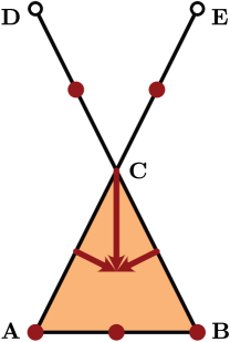
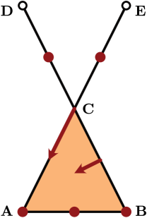
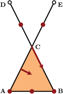
Figure 11. Three different multivector fields $\text{$\mathcal{V}$}_{0}$ (left), $\text{$\mathcal{V}$}_{1}$ (middle), and $\text{$\mathcal{V}$}_{2}$ (right) on the Lefschetz complex $X$ introduced in Example 3.17. Critical cells are marked with a fat circle in the center of mass of a simplex. Vectors and multivectors are indicated by an arrow from simplex $x$ to simplex $y$ whenever $y\in\Pi_{\text{$\mathcal{V}$}}(x)$ and $y\not\in\operatorname{cl}x$, and as long as $y$ is a top-dimensional coface in the multivector containing $x$. The remaining cases of arrows $x\to y$ are not marked in order to keep the image readable.

We call a subset $A\subset\mbox{$\mathbb{Z}$}$ left bounded (respectively right bounded) if it has a minimum (respectively maximum). Otherwise we call it left unbounded or left infinite (respectively right unbounded or right infinite). We call $A\subset\mbox{$\mathbb{Z}$}$ bounded if $A$ has both a minimum and a maximum. Finally, we call $A\subset\mbox{$\mathbb{Z}$}$ a $\mathbb{Z}$-interval if $A=\mbox{$\mathbb{Z}$}\cap I$ where $I$ is an interval in $\mathbb{R}$.

A solution of a multivector field $\mathcal{V}$ in $A\subset X$ is a partial map $\varrho:\mbox{$\mathbb{Z}$}\nrightarrow A$ whose domain, denoted by $\operatorname{dom}\varrho$, is a $\mathbb{Z}$-interval and for any $i,i+1\in\operatorname{dom}\varrho$ the inclusion $\varrho(i+1)\in\Pi_{\text{$\mathcal{V}$}}(\varrho(i))$ holds. The solution passes through $x\in X$ if $0\in\operatorname{dom}\varrho$ and $x=\varrho(0)$. The solution $\varrho$ is full if $\operatorname{dom}\varrho=\mbox{$\mathbb{Z}$}$. It is periodic if there is a $k>0$ such that $\varrho(i+k)=\varrho(i)$ for all $i\in\mbox{$\mathbb{Z}$}$. It is a partial solution or simply a path if $\operatorname{dom}\varrho$ is bounded. We refer to the cardinality of the domain of a path as the length of the path. If the maximum of $\operatorname{dom}\varrho$ exists, we call the value of $\varrho$ at this maximum the right endpoint of $\varrho$. If the minimum of $\operatorname{dom}\varrho$ exists, we call the value of $\varrho$ at this minimum the left endpoint of $\varrho$. We denote the left and right endpoints of $\varrho$ by $\varrho^{\sqsubset}$ and $\varrho^{\sqsupset}$, respectively. Given a full solution $\varrho$ through $x\in X$, we denote by $\varrho^{+}:=\varrho_{|\scriptsize{\mbox{$\mathbb{Z}$}}_{0}^{+}}$ the forward solution through $x$, and by $\varrho^{-}:=\varrho_{|\scriptsize{\mbox{$\mathbb{Z}$}}_{0}^{-}}$ the backward solution through $x$.

By a shift of a solution $\varrho$ we mean the composition $\varrho\circ\tau_{n}$, where the translation map is defined as $\tau_{n}:\mbox{$\mathbb{Z}$}\ni m\mapsto m+n\in\mbox{$\mathbb{Z}$}$. Given two solutions $\varphi$ and $\psi$ such that $\psi^{\sqsubset}$ and $\varphi^{\sqsupset}$ exist and $\psi^{\sqsubset}\in\Pi_{\text{$\mathcal{V}$}}(\varphi^{\sqsupset})$, there is a unique shift $\tau_{n}$ such that $\varphi\cup\psi\circ\tau_{n}$ is a solution. We call this union of paths the concatenation of $\varphi$ and $\psi$ and denote it $\varphi\cdot\psi$. We also identify each $x\in X$ with the path of length one whose image is $\{x\}$.

The following proposition is straightforward.

Proposition 7.3.

Let $x,y\in X$. Then $y\in\Pi_{\text{$\mathcal{V}$}}(x)$ if and only if there is an arrow from $[x]$ to $[y]$ in the $\mathcal{V}$-digraph. Consequently, the multivector field $\mathcal{V}$ admits a path from $x$ to $y$ if and only if there is a path from $[x]$ to $[y]$ in the $\mathcal{V}$-digraph. ∎

Finally, and for later reference, we define the backward and forward ultimate image of a full solution $\varrho:\mbox{$\mathbb{Z}$}\to X$, respectively, as the sets

$$\mbox{$\operatorname{uim}$}^{-}(\varrho) := \bigcap_{t\in\mbox{$\mathbb{Z}$}^{-}}\varrho((-\infty,t]),$$

$$\mbox{$\operatorname{uim}$}^{+}(\varrho) := \bigcap_{t\in\mbox{$\mathbb{Z}$}^{+}}\varrho([t,\infty)).$$

One can easily see that both of these sets are necessarily nonempty. Moreover, the following proposition is straightforward.

Proposition 7.4.

If $\varrho:\mbox{$\mathbb{Z}$}\to X$ is a periodic solution, then its backward and forward ultimate images satisfy $\mbox{$\operatorname{uim}$}^{-}(\varrho)=\operatorname{im}\varrho=\mbox{$\operatorname{uim}$}^{+}(\varrho)$. ∎

While the above notion of solution is a natural generalization of the classical case, the specific definition of the multivalued map $\Pi_{\text{$\mathcal{V}$}}$ causes some slight complication. Since we clearly have $x\in\Pi_{\text{$\mathcal{V}$}}(x)$ for every $x\in X$, every point in the Lefschetz complex lies on a constant full solution through itself. Thus, if we are interested in extending notions such as invariance from the classical situation, our concept of solution implies that every subset of $X$ would be an invariant set, which clearly is not appropriate. This can be remedied by strengthening our notion of solutions to the concept of essential solutions.

A full solution $\varrho:\mbox{$\mathbb{Z}$}\to X$ is called left-essential (or, respectively, right-essential), if for every regular $x\in\operatorname{im}\varrho$ the set $\{\,t\in\mbox{$\mathbb{Z}$}\mid\varrho(t)\not\in[x]_{\text{$\mathcal{V}$}}\,\}$ is left-infinite (or, respectively, right-infinite). We say that $\varrho$ is an essential solution if it is both left- and right-essential. In other words, essential solutions have to leave every regular multivector in forward and in backward time before they can re-enter it.

7.2. Conley index and Morse decompositions

We say that $S\subset X$ is $\mathcal{V}$-invariant, or briefly invariant, if for every $x\in S$ there exists an essential solution through $x$ in $S$. A closed set $N\subset X$ is an isolating set for a $\mathcal{V}$-invariant subset $S\subset N$ if $\Pi_{\text{$\mathcal{V}$}}(S)\subset N$ and any path in $N$ with endpoints in $S$ is a path in $S$. Finally, we say that $S$ is an isolated invariant set if $S$ admits an isolating set. One can show that isolated invariant sets have an easy direct characterization. This is the subject of the following proposition (see also [24, Propositions 4.10, 4.12, and 4.13]).

Proposition 7.5.

A subset $S\subset X$ is an isolated invariant set for $\mathcal{V}$ if and only if it is an invariant set which is both $\mathcal{V}$-compatible and locally closed.

Consider an isolated invariant set $S$ of a combinatorial multivector field $\mathcal{V}$ on a Lefschetz complex $X$. The Conley index of $S$ is defined in [24, Section 5.2] as the homology of any index pair of $S$, in particular the homology $H(\operatorname{cl}S,\operatorname{mo}S)$ of a special index pair $(\operatorname{cl}S,\operatorname{mo}S)$ (see [24, Theorem 5.3]). Since, in view of Proposition 3.19 and Proposition 7.5, $H(\operatorname{cl}S,\operatorname{mo}S)$ is isomorphic to $H(S)$, for the purposes of this paper it suffices to assume that the Conley index of an isolated invariant set $S$ is

$$\operatorname{Con}(S):=H(S),$$

that is, the Lefschetz homology of $S$.

Observe that given an isolated invariant set $S$ for a multivector field $\mathcal{V}$ on a Lefschetz complex $X$, by Proposition 7.5 the family

$$\text{$\mathcal{V}$}_{S}:=\mbox{$\{\,V\in\text{$\mathcal{V}$}\mid V\subset S\,\}$}$$

is a partition of $S$ and, in consequence, a multivector field on $S$ considered as a Lefschetz subcomplex of $X$. We call it the multivector field induced by $\mathcal{V}$ on $S$.

Multivector fields on Lefschetz complexes can exhibit a variety of different dynamical behaviors, ranging from critical cells which correspond to equilibrium solutions, to both transient and more complicated recurrent behavior. In this context, an essential, and therefore, full solution $\varrho:\mbox{$\mathbb{Z}$}\to X$ is called recurrent if for every $x\in\operatorname{im}\varrho$ the set $\varrho^{-1}(x)$ is both left- and right-infinite. Examples of recurrent solutions include constant solutions whose image is a single critical multivector, or nonconstant periodic solutions which loop through a sequence of regular multivectors.

In classical dynamics, one has the notion of a gradient vector field, which rules out the existence of nonconstant recurrent solutions — and in fact, Forman’s original combinatorial vector fields were motivated by precisely this situation. While our definition of combinatorial multivector fields is considerably more general and allows for recurrence, we will see that assuming an additional gradient structure can provide more detailed information about the associated connection matrices.

Thus, we call a multivector field $\mathcal{V}$ gradient-like if for every recurrent solution $\varrho:\mbox{$\mathbb{Z}$}\to X$ there exists a multivector $V\in\text{$\mathcal{V}$}$ such that $\operatorname{im}\varrho\subset V$. Moreover, a multivector field $\mathcal{V}$ is called a gradient multivector field if the only recurrent solutions are constant solutions with its value in a singleton of $\mathcal{V}$. We would like to point out that this rules out multivectors of size at least two which have nontrivial Conley index. Moreover, recall that a singleton in $\mathcal{V}$ is always critical, see Proposition 3.20.

Gradient-like multivector fields on Lefschetz complexes are of significant importance on our theory of connection matrices, since they correspond precisely to acyclic partitions. This is the subject of the following result.

Proposition 7.6.

Let $\mathcal{V}$ be a combinatorial multivector field on a Lefschetz complex $X$. The following properties are equivalent.

• The multivector field $\mathcal{V}$ is gradient-like.

• After discarding self-loops, the $\mathcal{V}$-digraph is acyclic.

• The collection $\mathcal{V}$ of multivectors is an acyclic partition of $X$.

Proof: The equivalence (i)$\;\Leftrightarrow\;$(ii) follows from Proposition 7.3, and the equivalence (ii)$\;\Leftrightarrow\;$(iii) follows from Proposition 7.1. ∎

In order to define connection matrices for multivector fields on a Lefschetz complex $X$ we need the concept of a Morse decomposition of an isolated invariant set. Let $S$ be an isolated invariant set of a multivector field $\mathcal{V}$ on a Lefschetz complex $X$. By Morse decomposition of $S$ we mean in this paper a collection $\mathcal{M}$ of mutually disjoint, non-empty isolated invariant subsets of $S$, referred to as Morse sets, together with a partial order $\leq$ on $\mathcal{M}$ such that for every essential solution $\varrho:\mbox{$\mathbb{Z}$}\to S$ one either has $\operatorname{im}\varrho\subset M$ for a Morse set $M\in\text{$\mathcal{M}$}$, or there exist two Morse sets $M^{\pm}\in\text{$\mathcal{M}$}$ with $M^{+}<M^{-}$ and for which $\mbox{$\operatorname{uim}$}^{-}(\varrho)\subset M^{-}$ and $\mbox{$\operatorname{uim}$}^{+}(\varrho)\subset M^{+}$ are satisfied. By a Morse decomposition of $\mathcal{V}$ we mean a Morse decomposition of the maximal invariant subset of $\mathcal{V}$ in $X$.

We would like to point out that this definition of Morse decomposition differs in two aspects from the one given in [24]. The definition in [24], instead of the condition with $\mbox{$\operatorname{uim}$}^{-}(\varrho)$ and $\mbox{$\operatorname{uim}$}^{+}(\varrho)$, uses the condition with $\alpha$- and $\omega$-limit sets of $\varrho$. The reader familiar with [24] will, however, immediately notice that these conditions are equivalent, in view of Proposition 7.5. Also, paper [24] defines a global Morse decomposition, that is a Morse decomposition of the whole space $X$ instead of an isolated invariant set $S$ of $\mathcal{V}$ in $X$. Since the definition in [24] is given under the assumption that $X$ is invariant, one can easily regain the definition of Morse decomposition of an isolated invariant set $S$ from the definition in [24] by replacing $X$ with $S$ and $\mathcal{V}$ with the multivector field $\text{$\mathcal{V}$}_{S}$ induced by $\mathcal{V}$ on $S$. Global Morse decompositions of a combinatorial multivector field can easily be determined via the strongly connected components of the associated $\mathcal{V}$-digraph. In fact, in contrast to the classical case, there always exists a finest Morse decomposition for $\mathcal{V}$.

In our definition of Morse decomposition we assume that all Morse sets are non-empty. Although this is in the spirit of the classical definition by Conley [6], in terms of computational applications the assumption may be inconvenient, because there may be areas where it is impossible to decide whether they contain a non-empty invariant set due to limited data or computational power. As a remedy to this situation we define connection matrices for block decompositions, a concept slightly more general than Morse decompositions.

Definition 7.7.

Let $\mathcal{V}$ be a combinatorial multivector field on a Lefschetz complex $X$ and let $S\subset X$ be an isolated invariant set. A block in $S$ is a locally closed and $\mathcal{V}$-compatible subset of $S$. A block decomposition of $S$ is a family $\mathcal{M}$ of mutually disjoint, non-empty blocks in $S$, together with a partial order $\leq$ on $\mathcal{M}$ and such that:

• If $\tau$ is a path in $S$ with $\tau^{\sqsubset}\in M$ and $\tau^{\sqsupset}\in M^{\prime}$ for some $M,M^{\prime}\in\text{$\mathcal{M}$}$, then $M\geq M^{\prime}$, and additionally $M=M^{\prime}$ implies $\operatorname{im}\tau\subset M=M^{\prime}$.

• For every essential solution $\varrho\in S$ the set $\varrho^{-1}\left(\bigcup\text{$\mathcal{M}$}\right)$ is left and right infinite.

It follows from Proposition 7.5 that every isolated invariant set is a block. A block does not have to be an isolated invariant set, because it may fail to be invariant. But, if $B$ is a block, then one can easily verify that

$$\operatorname{Inv}B:=\mbox{$\{\,x\in B\mid\text{there is an essential solution through $x$ in $B$}\,\}$}$$

is invariant, locally closed, and $\mathcal{V}$-compatible, hence an isolated invariant set, again by Proposition 7.5. We leave the proof of the following simple proposition to the reader.

Proposition 7.8.

If $\mathcal{M}$ is a Morse decomposition of $S$ then it is also a block decomposition of $S$. Conversely, if $\mathcal{M}$ is a block decomposition of $S$, then

(89) $$\text{$\mathcal{M}$}^{\bullet}:=\mbox{$\{\,\operatorname{Inv}M\mid M\in\text{$\mathcal{M}$},\,\operatorname{Inv}M\neq\varnothing\,\}$}$$

is a Morse decomposition of $S$. ∎

The problem with potentially empty invariant sets in a Morse decomposition is also addressed in [19], and our proposed concept of block decomposition fits well with the solution of this reference. The reader familiar with the terminology of [19] will easily notice that given a block decomposition $\mathcal{N}$, the family $\text{$\mathcal{M}$}:=\text{$\mathcal{N}$}^{\bullet}$ becomes a Morse representation in the sense of [19], and the order embedding $\text{$\mathcal{M}$}\to\text{$\mathcal{N}$}$ which sends a nonempty invariant set $M\in\text{$\mathcal{M}$}$ to the unique block $N\in\text{$\mathcal{N}$}$ containing $M$ is then a Morse decomposition in their sense.

It is often convenient to consider a Morse or block decomposition as a family $\text{$\mathcal{M}$}=\{M_{p}\mid p\in P\}$ indexed by a poset $P$ with the partial order in $\mathcal{M}$ given by

(90) $$M_{r}\leq M_{s}\;\Leftrightarrow\;r\leq s.$$

A block decomposition $\mathcal{M}$ shares with a Morse decomposition its crucial property, as the following proposition shows.

Proposition 7.9.

Assume that $\text{$\mathcal{M}$}=\{M_{p}\}_{p\in P}$ is a block decomposition of an isolated invariant set $S$. Then for every essential solution $\varrho$ in $S$ there exist $p^{-},p^{+}\in P$ such that $p^{-}\geq p^{+}$ and

(91) $$\mbox{$\operatorname{uim}$}^{-}\varrho\subset M_{p^{-}}\quad\mbox{and}\quad\mbox{$\operatorname{uim}$}^{+}\varrho\subset M_{p^{+}}.$$

Moreover, if $p^{-}=p^{+}$, then one also has

(92) $$\operatorname{im}\varrho\subset M_{p^{-}}.$$

Proof: It follows from (BD1) that

$$P_{\varrho}:=\mbox{$\{\,p\in P\mid M_{p}\cap\operatorname{im}\varrho\neq\varnothing\,\}$}$$

is a linearly ordered subset of $P$. Set $p^{-}:=\max P_{\varrho}$, $p^{+}:=\min P_{\varrho}$ and choose $k^{-},k^{+}\in\mbox{$\mathbb{Z}$}$ such that $\varrho(k^{-})\in M_{p^{-}}$, $\varrho(k^{+})\in M_{p^{+}}$. We claim that

(93) $$\varrho([k^{+},\infty))\subset M_{p^{+}}.$$

To see this, assume to the contrary that $\varrho(n)\not\in M_{p^{+}}$ for some $n>k^{+}$. Since, by (BD2), the preimage $\varrho^{-1}\left(\bigcup\text{$\mathcal{M}$}\right)$ is right infinite, there exists an index $m>n$ such that $\varrho(m)\in\bigcup\text{$\mathcal{M}$}$. Then $\varrho(m)\in M_{p^{+}}$, because otherwise we contradict the definition of $p^{+}$. Consider now the path $\tau:=\varrho_{|[k^{+},m]}$. We have $\tau^{\sqsubset}=\varrho(k^{+})\in M_{p^{+}}$ and $\tau^{\sqsupset}=\varrho(m)\in M_{p^{+}}$. Hence, we get from (BD1) that $\varrho(n)=\tau(n)\in\operatorname{im}\tau\subset M_{p^{+}}$, a contradiction proving (93). Similarly we prove that

(94) $$\varrho((-\infty,k^{-}])\subset M_{p^{-}}.$$

Consider now the case $k^{-}\geq k^{+}$. Applying (BD1) to $\sigma:=\varrho_{|[k^{+},k^{-}]}$ we obtain the inequality $p^{+}\geq p^{-}$, which in turn forces the equality $p^{+}=p^{-}$, because we have $p^{+}=\min\ P_{\varrho}\leq\max\ P_{\varrho}=p^{-}$. We also get from (93) and (94) that

$$\operatorname{im}\varrho\subset\varrho((-\infty,k^{-}])\cup\varrho([k^{+},\infty))\subset M_{p^{-}},$$

which shows that $\varrho$ satisfies (92). Hence, this solution also satisfies (91), because $\mbox{$\operatorname{uim}$}^{-}\varrho\subset\operatorname{im}\varrho$ and $\mbox{$\operatorname{uim}$}^{+}\varrho\subset\operatorname{im}\varrho$. This completes the proof in the case $k^{-}\geq k^{+}$.

Consider finally the case $k^{-}<k^{+}$. Then, again by (BD1), one has the inequality $p^{-}\geq p^{+}$, together with $\mbox{$\operatorname{uim}$}^{-}\varrho\subset\varrho((-\infty,k^{-}])\subset M_{p^{-}}$ by (94), as well as $\mbox{$\operatorname{uim}$}^{+}\varrho\subset\varrho([k^{+},\infty))\subset M_{p^{+}}$ by (93). Hence, $\varrho$ satisfies (91). Moreover, if $p^{-}=p^{+}$, then

$$\operatorname{im}\varrho\subset\varrho((-\infty,k^{-}])\cup\varrho([k^{-},k^{+}])\cup\varrho([k^{+},\infty))\subset M_{p^{+}},$$

which shows that $\varrho$ satisfies (91) when $p^{-}=p^{+}$. ∎

Corollary 7.10.

Assume $\text{$\mathcal{M}$}=\{M_{p}\}_{p\in P}$ is a block decomposition of an isolated invariant set $S$. Then every multivector $V\not\in\bigcup\text{$\mathcal{M}$}$ is regular.

Proof: Assume, to the contrary, that $V\not\in\bigcup\text{$\mathcal{M}$}$ is critical. Let $\varrho$ be a constant, full solution through an element $x\in V$. Then $\varrho$ is essential and $\mbox{$\operatorname{uim}$}^{-}\varrho=\mbox{$\operatorname{uim}$}^{+}\varrho=\{x\}=\operatorname{im}\varrho$. Hence, by Proposition 7.9 there is a $p\in P$ such that $\operatorname{im}\varrho\subset M_{p}$. It follows that $V\subset M_{p}$, a contradiction. ∎

Let $\mathcal{M}$ be a Morse or block decomposition of $\mathcal{V}$. Then the family

$$\text{$\mathcal{M}$}\cup\mbox{$\{\,V\in\text{$\mathcal{V}$}\mid V\cap\bigcup\text{$\mathcal{M}$}=\varnothing\,\}$}$$

is clearly a partition of $X$. We call it the partition induced by the decomposition $\mathcal{M}$ and denote it $\text{$\mathcal{E}$}_{\text{$\mathcal{M}$},\text{$\mathcal{V}$}}$, or just $\text{$\mathcal{E}$}_{\text{$\mathcal{M}$}}$ when $\mathcal{V}$ is clear from the context. Each $E\in\text{$\mathcal{E}$}_{\text{$\mathcal{M}$}}$ is either a block, or it is a multivector which is not contained in any of the blocks. For two sets $E,E^{\prime}\in\text{$\mathcal{E}$}_{\text{$\mathcal{M}$}}$ we write $E\preccurlyeq E^{\prime}$ if and only if there is a path $\sigma$ such that $\sigma^{\sqsubset}\in E^{\prime}$ and $\sigma^{\sqsupset}\in E$. Then the following statement holds.

Proposition 7.11.

The relation $\preccurlyeq$ is a partial order in $\text{$\mathcal{E}$}_{\text{$\mathcal{M}$}}$.

Proof: Clearly, the relation is reflexive and transitive. To see that it is antisymmetric, take $E,E^{\prime}\in\text{$\mathcal{E}$}_{\text{$\mathcal{M}$}}$ such that $E\preccurlyeq E^{\prime}$ and $E^{\prime}\preccurlyeq E$. We have to prove that $E=E^{\prime}$. Let $\sigma$ be a path such that $\sigma^{\sqsubset}\in E^{\prime}$ and $\sigma^{\sqsupset}\in E$. In addition, let $\tau$ denote a path which satisfies both $\tau^{\sqsubset}\in E$ and $\tau^{\sqsupset}\in E^{\prime}$.

Consider first the case when $E$ and $E^{\prime}$ are multivectors disjoint from $\bigcup\text{$\mathcal{M}$}$. Then $[\sigma^{\sqsubset}]=E^{\prime}=[\tau^{\sqsupset}]$ and $[\sigma^{\sqsupset}]=E=[\tau^{\sqsubset}]$. It follows that the paths $\sigma$ and $\tau$ can be concatenated to a full, periodic solution $\varrho$. Assume now that we have $E\neq E^{\prime}$. Then the solution $\varrho$ is essential. Hence, by Proposition 7.9 we can find $p^{-},p^{+}\in P$ such that $p^{-}\geq p^{+}$, $\mbox{$\operatorname{uim}$}^{-}\varrho\subset M_{p^{-}}$ and $\mbox{$\operatorname{uim}$}^{+}\varrho\subset M_{p^{+}}$. However, it follows from Proposition 7.4 that $\mbox{$\operatorname{uim}$}^{-}(\varrho)=\operatorname{im}\varrho=\mbox{$\operatorname{uim}$}^{+}(\varrho)$. Therefore, we must have $p^{-}=p^{+}$. In consequence, $\sigma^{\sqsubset}\in E^{\prime}\cap M_{p^{-}}$, which contradicts our assumption that both $E$ and $E^{\prime}$ are multivectors disjoint from $\bigcup\text{$\mathcal{M}$}$. Thus, we have $E=E^{\prime}$ in this case.

Consider now the case when both $E$ and $E^{\prime}$ are in $\mathcal{M}$. Then $E=M_{p}$ and $E^{\prime}=M_{p^{\prime}}$ for some $p,p^{\prime}\in P$. Hence, applying (BD1) to $\sigma$ we obtain the inequality $p^{\prime}\geq p$, and after applying (BD1) to $\tau$ we further get $p\geq p^{\prime}$. It follows that $p=p^{\prime}$ and $E=M_{p}=M_{p^{\prime}}=E^{\prime}$.

Finally, consider the case when one of the sets $E$, $E^{\prime}$ is in $\mathcal{M}$ and the other is a multivector disjoint from $\bigcup\text{$\mathcal{M}$}$. Without loss of generality we may assume that $E=M_{p}$ for some $p\in P$ and $E^{\prime}\cap\bigcup\text{$\mathcal{M}$}=\varnothing$. Then we have $[\sigma^{\sqsubset}]=E^{\prime}=[\tau^{\sqsupset}]$. It follows that the paths $\sigma$ and $\tau$ can be concatenated to a path $\pi$ such that $\pi^{\sqsubset}=\tau^{\sqsubset}\in M_{p}$ and $\pi^{\sqsupset}=\sigma^{\sqsupset}\in M_{p}$. Applying (BD1) to $\pi$ we obtain the inclusion $\operatorname{im}\pi\subset M_{p}=E$. Since $\sigma^{\sqsubset}\in\operatorname{im}\pi$ and $\sigma^{\sqsubset}\in E^{\prime}$, we get $E\cap E^{\prime}\neq\varnothing$ which implies $E=E^{\prime}$, because $\text{$\mathcal{E}$}_{\text{$\mathcal{M}$}}$ is a partition. ∎

Since $\text{$\mathcal{E}$}_{\text{$\mathcal{M}$}}$ is a partition of the Lefschetz complex, one can also consider the relation $\preceq_{\text{$\mathcal{E}$}_{\text{$\mathcal{M}$}}}$ defined in (72). As the following result demonstrates, its transitive closure is the partial order $\preccurlyeq$ from above.

Proposition 7.12.

The relation $\preccurlyeq$ is the transitive closure of the relation $\preceq_{\text{$\mathcal{E}$}_{\text{$\mathcal{M}$}}}$ defined in (72). Thus, the two relations $\preccurlyeq$ and $\leq_{\text{$\mathcal{E}$}_{\text{$\mathcal{M}$}}}$ coincide, and in particular, the family $\text{$\mathcal{E}$}_{\text{$\mathcal{M}$}}$ is an acyclic partition of $X$.

Proof: We need to prove that for all $E,E^{\prime}\in\text{$\mathcal{E}$}_{\text{$\mathcal{M}$}}$ one has the equivalence

(95) $$E\leq_{\text{$\mathcal{E}$}_{\text{$\mathcal{M}$}}}E^{\prime}\quad\;\Leftrightarrow\;\quad E\preccurlyeq E^{\prime}.$$

First, we will prove that

(96) $$E\cap\operatorname{cl}E^{\prime}\neq\varnothing\quad\;\Rightarrow\;\quad E\preccurlyeq E^{\prime}.$$

Let $x\in E\cap\operatorname{cl}E^{\prime}$ be arbitrary. Then $x\in\operatorname{cl}y$ for a $y\in E^{\prime}$. Thus, $\sigma:=y\cdot x$ is a path. Moreover, $\sigma^{\sqsubset}=y\in E^{\prime}$ and $\sigma^{\sqsupset}=x\in E$, proving (96). Since, by Proposition 7.11, the relation $\preccurlyeq$ is transitive, it follows from property (96) that the left-hand side of (95) implies the right-hand side of (95).

For the reverse implication assume that $E\preccurlyeq E^{\prime}$. Let $\varrho=x_{0}\cdot x_{1}\cdot\ldots\cdot x_{n}$ be a path from $E^{\prime}$ to $E$. Let $V_{i}:=[x_{i}]$. Then $V_{0}\subset E^{\prime}$ and $V_{n}\subset E$. Moreover, since $x_{i+1}\in\operatorname{cl}x_{i}\cup[x_{i}]$, we see that $V_{i+1}\cap\operatorname{cl}V_{i}\neq\varnothing$ or $V_{i+1}=V_{i}$. It follows that $V_{i+1}\preceq_{\text{$\mathcal{E}$}_{\text{$\mathcal{M}$}}}V_{i}$, and therefore $E\leq_{\text{$\mathcal{E}$}_{\text{$\mathcal{M}$}}}E^{\prime}$. Thus, (95) is proved. Hence, it follows from Proposition 7.11 that $\leq_{\text{$\mathcal{E}$}_{\text{$\mathcal{M}$}}}$ is a partial order on $\text{$\mathcal{E}$}_{\text{$\mathcal{M}$}}$, and this finally implies that $\text{$\mathcal{E}$}_{\text{$\mathcal{M}$}}$ is an acyclic partition. ∎

Proposition 7.12 lets us consider $(\text{$\mathcal{E}$}_{\text{$\mathcal{M}$}},\preccurlyeq)$ as a poset. We also consider it as an object of DPSet with the distinguished subset given by

$$(\text{$\mathcal{E}$}_{\text{$\mathcal{M}$}})_{\star}:=\text{$\mathcal{M}$}.$$

Note that such a definition of $(\text{$\mathcal{E}$}_{\text{$\mathcal{M}$}})_{\star}$ satisfies (34), because it follows from Corollary 7.10 that every $V\in\text{$\mathcal{V}$}\setminus\bigcup\text{$\mathcal{M}$}$ must be regular which implies that $C(V)$ is inessential.

7.3. Connection matrices and heteroclinics

After these preparations, Proposition 7.12 finally enables us to define the Conley complex and associated connection matrix of a given Morse or block decomposition.

Definition 7.13.

The Conley complex and the associated connection matrix of a Morse or block decomposition $\mathcal{M}$ of a combinatorial multivector field $\mathcal{V}$ on a Lefschetz complex $X$ is defined as the Conley complex and the associated connection matrix of the acyclic partition $\text{$\mathcal{E}$}_{\text{$\mathcal{M}$}}$, i.e., the Conley complex and respective connection matrix of the poset filtered chain complex $(\text{$\mathcal{E}$}_{\text{$\mathcal{M}$}},C(X),{\bf\partial}^{\kappa})$.

Example 7.14.

All three combinatorial multivector fields $\text{$\mathcal{V}$}_{0}$, $\text{$\mathcal{V}$}_{1}$, $\text{$\mathcal{V}$}_{2}$ in Figure 11 have a common Morse decomposition given as the family

$$\{\{\mathbf{A}\},\{\mathbf{B}\},\{\mathbf{AB}\},\{\mathbf{CD}\},\{\mathbf{CE}\}\},$$

which consists of singletons. However, the acyclic partition $\text{$\mathcal{E}$}_{i}:=\text{$\mathcal{E}$}_{\text{$\mathcal{M}$},\text{$\mathcal{V}$}_{i}}$ is different for each index $i\in\{0,1,2\}$. In these simple examples, $\text{$\mathcal{E}$}_{i}$ coincides with $\text{$\mathcal{V}$}_{i}$. The filtered chain complex $(\text{$\mathcal{E}$}_{0},C(X),\partial^{\kappa})$ coincides with the filtered chain complex considered in Example 4.15. Therefore, the connection matrices given by (41) and (68) are the connection matrices of $\mathcal{M}$ for $\text{$\mathcal{V}$}_{0}$. We know that these matrices are not equivalent. $\Diamond$

For a subfamily $\text{$\mathcal{L}$}\subset\text{$\mathcal{M}$}$ we define $M(\text{$\mathcal{L}$})$ as the collection of cells $x\in X$ for which there exists an essential solution $\varrho$ through $x$ and $M_{-},M_{+}\in\text{$\mathcal{L}$}$ such that $\mbox{$\operatorname{uim}$}^{-}(\varrho)\subset M^{-}$ and $\mbox{$\operatorname{uim}$}^{+}(\varrho)\subset M^{+}$.

Proposition 7.15.

The set $M(\text{$\mathcal{L}$})\subset X$ is an isolated invariant set for $\mathcal{V}$. Moreover, $\mathcal{L}$ is a Morse decomposition of $M(\text{$\mathcal{L}$})$.

Proof: The first statement is the contents of [24, Theorem 7.4]. The second statement is straightforward. ∎

As an immediate consequence of Theorem 5.15 and Corollary 5.16 we obtain the following proposition.

Proposition 7.16.

Assume $(\text{$\mathcal{M}$},\bar{C},\bar{d})$ is a Conley complex of a Morse decomposition $\mathcal{M}$ of an isolated invariant set $S$. If $\text{$\mathcal{L}$}\subset\text{$\mathcal{M}$}$ is convex with respect to the partial order $\leq$ in $\mathcal{M}$, then $(\text{$\mathcal{L}$},\bar{C}_{\text{$\mathcal{L}$}},\bar{d}_{\text{$\mathcal{L}$}\text{$\mathcal{L}$}})$ is a Conley complex of $\mathcal{L}$ considered as a Morse decomposition of $M(\text{$\mathcal{L}$})$. Moreover, the Conley index of $M(\text{$\mathcal{L}$})$ is isomorphic to $H(\bar{C}_{\text{$\mathcal{L}$}},\bar{d}_{\text{$\mathcal{L}$}\text{$\mathcal{L}$}})$. ∎

Clearly, every singleton $\{M\}\subset\text{$\mathcal{M}$}$, consisting of just one Morse set $M$, is convex in $\mathcal{M}$. Since, by the definition of Conley complex, $\bar{d}_{MM}=0$, we get the following corollary from Proposition 7.15.

Corollary 7.17.

Given a Conley complex $(\text{$\mathcal{M}$},\bar{C},\bar{d})$ of a Morse decomposition $\mathcal{M}$ of an isolated invariant set $S$ of $\mathcal{V}$, the Conley index $\operatorname{Con}(M)$ is isomorphic to $\bar{C}_{M}$ for every $M\in\text{$\mathcal{M}$}$. ∎

In terms of applications, the most important result of classical connection matrix theory states that if $\{M_{p}\}_{p\in P}$ is a Morse decomposition indexed by a poset $P$ and $p,q\in P$ are such that $q$ covers $p$ and the entry in the $q$th row and $p$th column of the connection matrix is non-zero, then there must be a heteroclinic connection running from $M_{q}$ to $M_{p}$. We have an analogous result for combinatorial multivector fields.

Let $(\text{$\mathcal{M}$},\bar{C},\bar{d})$ be a Conley complex of a Morse decomposition $\text{$\mathcal{M}$}=\{M_{p}\}_{p\in P}$. Denote by $A$ the associated connection matrix. Then $A$ may be viewed as a block matrix $[A_{rs}]_{r,s\in P}$ by identifying $P$ with $\mathcal{M}$.

Theorem 7.18.

Consider $p,q\in P$ such that $p<q$ and $\{p,q\}$ is convex in $P$. If $A_{pq}\neq 0$, then there is a heteroclinic connection from $M_{q}$ to $M_{p}$, that is an essential solution $\varrho$ satisfying

(97) $$\mbox{$\operatorname{uim}$}^{-}(\varrho)\subset M_{q}\quad\text{ and }\quad\mbox{$\operatorname{uim}$}^{+}(\varrho)\subset M_{p}.$$

Proof: Assume to the contrary that there is no heteroclinic connection from $M_{q}$ to $M_{p}$. Set $M_{pq}:=M(\{M_{p},M_{q}\})$. It follows from Proposition 7.15 that $M_{pq}$ is an isolated invariant set with Morse decomposition $\{M_{p},M_{q}\}$. We will prove that

(98) $$M_{pq}=M_{p}\cup M_{q}.$$

For this, consider an arbitrary $x\in M_{pq}$. By the definition of $M_{pq}$, there are $M_{-},M_{+}\in\{M_{p},M_{q}\}$ and an essential solution $\varrho$ through $x$ in $M_{pq}$ such that $\mbox{$\operatorname{uim}$}^{-}(\varrho)\subset M^{-}$ and $\mbox{$\operatorname{uim}$}^{+}(\varrho)\subset M^{+}$. We cannot have $M_{-}=M_{p}$ and $M_{+}=M_{q}$, because then $M_{p}>M_{q}$, and by (90) we get $p>q$, which contradicts assumption $p<q$. We also cannot have $M_{-}=M_{q}$ and $M_{+}=M_{p}$, because otherwise $\varrho$ would be a heteroclinic connection from $M_{q}$ to $M_{p}$. Hence, either $M_{-}=M_{+}=M_{p}$ or $M_{-}=M_{+}=M_{q}$. Since $\{M_{p},M_{q}\}$ is a Morse decomposition of $M_{pq}$, in the fist case we get $x\in\operatorname{im}\gamma\subset M_{p}$ and in the second case we get $x\in\operatorname{im}\gamma\subset M_{q}$. This proves that $M_{pq}\subset M_{p}\cup M_{q}$. Since the opposite inclusion is obvious, the proof of (98) is completed. We also have

(99) $$M_{q}\cap\operatorname{cl}M_{p}=\varnothing,$$

(100) $$M_{p}\cap\operatorname{cl}M_{q}=\varnothing.$$

Indeed, to prove (99) assume to the contrary that $M_{q}\cap\operatorname{cl}M_{p}\neq\varnothing$. Then $\partial^{\kappa}_{M_{q}M_{p}}\neq 0$, which gives $M_{q}<M_{p}$, because $\partial^{\kappa}$ is filtered. But then $q<p$, which contradicts assumption $p<q$. To see (100) assume to the contrary that there is an $x\in M_{p}\cap\operatorname{cl}M_{q}$. Then $x\in\operatorname{cl}y$ for some $y\in M_{q}$ and since $M_{p}\neq\varnothing\neq M_{q}$, we can find an essential solution $\gamma_{q}$ through $y$ in $M_{q}$ and $\gamma_{p}$ through $x$ in $M_{p}$. Then $\gamma_{q}^{-}\cdot\gamma_{p}^{+}$ is a heteroclinic connection from $M_{q}$ to $M_{p}$, a contradiction.

It follows from (98-100) that $M_{pq}$, $M_{p}$, $M_{q}$ satisfy the assumptions of [24, Theorem 5.19]. This lets us conclude that

$$\operatorname{Con}(M_{pq})=\operatorname{Con}(M_{p})\oplus\operatorname{Con}(M_{q})$$

and, in consequence, that

(101) $$n_{pq}=n_{p}+n_{q}$$

where $n_{pq}$, $n_{p}$ and $n_{q}$ denote respectively the dimension of $\operatorname{Con}(M_{pq})$, $\operatorname{Con}(M_{p})$ and $\operatorname{Con}(M_{q})$. However, from Proposition 7.16 we know that the block matrix

$$\bar{A}_{pq}:=\left[\begin{array}[]{cc}0&A_{pq}\\ 0&0\end{array}\right]$$

is a connection matrix of the Conley complex for the Morse decomposition $\{M_{p},M_{q}\}$ of $M_{pq}$ and $\operatorname{Con}(M_{pq})$ is isomorphic to the homology of the Conley complex of the Morse decomposition $\mathcal{M}$ restricted to $\{M_{p},M_{q}\}$. By Corollary 7.17 we know that the $2\times 2$ block matrix $\bar{A}_{pq}$ has exactly $n_{p}$ columns in the first block and $n_{q}$ columns in the second block. Since $A_{pq}\neq 0$, we see that the kernel of $\bar{A}_{pq}$ is of dimension less than $n_{p}+n_{q}$. Therefore, the dimension of the homology of the restricted Conley complex and, in consequence, also the dimension of $\operatorname{Con}(M_{pq})$ is less than $n_{p}+n_{q}$, which contradicts (101) and proves the theorem. ∎

8. Connection matrices for Forman’s gradient vector fields

This last theoretical section of the paper is devoted to the study of the special case of Forman’s gradient vector fields on regular Lefschetz complexes. In this situation, one can show that the associated connection matrix is uniquely determined, and in fact can be determined in a direct way. This is accomplished in a number of steps. We begin by recalling basic properties of combinatorial vectors in the sense of Forman, before we present the definition and basic properties of his concept of combinatorial flow. After discussing the long-term limit of the latter, we can finally explain how it can be used to obtain the unique connection matrix in this setting. The uniqueness part of the assertion will rely heavily on the singleton partition which has already been discussed in Section 6.2.

8.1. Forman’s combinatorial flow

In the following, we assume that $\mathcal{V}$ is a gradient combinatorial vector field in the sense of Forman on a Lefschetz complex $X$. In terms of its definition, we recall that a combinatorial vector is just a combinatorial multivector $W$ with $\operatorname{card}W\leq 2$. A combinatorial multivector field whose multivectors are just vectors is then called a combinatorial vector field, a concept originally introduced by Forman [11, 12] in a slightly different but equivalent form. In the case of a combinatorial vector field the critical vectors are precisely the singletons, and the regular vectors are precisely the doubletons, i.e., vectors of cardinality two (see Proposition 3.20). Therefore, every gradient-like combinatorial vector field is a gradient combinatorial vector field.

Let $\text{$\mathcal{C}$}\subset\text{$\mathcal{V}$}$ denote the collection of critical vectors in $\mathcal{V}$. Since we assume that $\mathcal{V}$ is a combinatorial vector field, it follows from Proposition 3.20 that $\mathcal{C}$ is exactly the collection of singletons in $\mathcal{V}$. Moreover, the following proposition is straightforward.

Proposition 8.1.

Assume that $\mathcal{V}$ is a gradient combinatorial vector field. Then the collection $\mathcal{C}$ is a Morse decomposition of $\mathcal{V}$ and the induced acyclic partition of the Lefschetz complex $X$ is given by $\text{$\mathcal{E}$}_{\text{$\mathcal{C}$}}=\text{$\mathcal{V}$}$. ∎

It follows that the Conley complex of the Morse decomposition $\mathcal{C}$ of $X$ is the Conley complex of the filtered chain complex $(\text{$\mathcal{V}$},C(X),{\bf\partial}^{\kappa})$. The aim of this section is to prove that the Morse decomposition $\mathcal{C}$ has precisely one connection matrix, and that this connection matrix coincides with the matrix of the boundary operator of the associated Morse complex, see also [12, Section 7]. In order to make this statement precise, we first need to recall some concepts, with the current subsection focusing on properties of combinatorial vectors.

Unlike a general multivector, a combinatorial vector $W\in\text{$\mathcal{V}$}$ contains a unique minimal element and a unique maximal element in $W$ with respect to the face relation $\leq_{\kappa}$. We denote them by $W^{-}$ and $W^{+}$, respectively, and we extend this notation to cells by writing $x^{-}:=[x]^{-}$ and $x^{+}:=[x]^{+}$. Note that a combinatorial vector is given by $W=\{W^{-},W^{+}\}$, and $W$ is critical if and only if we have $W^{+}=W^{-}$, which in turn is equivalent to assuming that $W$ is a singleton. As a consequence of Proposition 3.15 one obtains for a vector $W$ the inequality

(102) $$0\leq\dim W^{+}-\dim W^{-}\leq 1,$$

and for all $x\in W$ one has

(103) $$\dim W^{-}\leq\dim x\leq\dim W^{+}.$$

We say that a cell $x$ is a tail if $x=x^{-}\neq x^{+}$ and a head if $x=x^{+}\neq x^{-}$. Clearly, if a cell is neither a tail nor a head, then it is critical. We denote the subsets of critical cells, tails, and heads by $X^{c}(\text{$\mathcal{V}$})$, $X^{-}(\text{$\mathcal{V}$})$, and $X^{+}(\text{$\mathcal{V}$})$, respectively, and shorten this notation to $X^{c}$, $X^{-}$, and $X^{+}$ whenever $\mathcal{V}$ is clear from context. Note that the collection $\mathcal{C}$ of critical vectors of $\mathcal{V}$ is precisely $\{\,\{x\}\mid x\in X^{c}\,\}$.

For a combinatorial vector $V\in\text{$\mathcal{V}$}$ we set $\dim V:=\dim V^{+}$. Moreover, recall that $\mathcal{V}$, as a gradient vector field, is an acyclic partition of $X$ according to Proposition 7.6. In particular, the collection $\mathcal{V}$ is a poset with the partial order $\leq_{\text{$\mathcal{V}$}}$. Then one has the following proposition.

Proposition 8.2.

Assume that $\mathcal{V}$ is a gradient vector field on a Lefschetz complex $X$. Then the following hold:

• The map $\dim:(\text{$\mathcal{V}$},\leq_{\text{$\mathcal{V}$}})\to(\mbox{$\mathbb{N}$}_{0},\leq)$ is order preserving.

• If $V<_{\text{$\mathcal{V}$}}W$ and $V$ is critical, then $\dim V<\dim W$.

• The choice $\text{$\mathcal{V}$}_{\star}=\text{$\mathcal{C}$}$ is possible, since the set of $V\in\text{$\mathcal{V}$}$ such that $C(V)$ is homotopically essential coincides with the set of critical vectors $\mathcal{C}$.

Proof: Since, by definition, the relation $\leq_{\text{$\mathcal{V}$}}$ is the transitive closure of the relation $\preceq_{\text{$\mathcal{V}$}}$, to prove (i) it suffices to verify that $V\cap\operatorname{cl}W\neq\varnothing$ for $V,W\in\text{$\mathcal{V}$}$ implies $\dim V\leq\dim W$. Thus, assume that $V\cap\operatorname{cl}W\neq\varnothing$. Let $x\in V\cap\operatorname{cl}W$. If $x\in W$, then $V\cap W\neq\varnothing$ which implies $V=W$, because $\mathcal{V}$ is a partition. In particular, this gives $\dim V=\dim W$. Thus, consider now case $x\not\in W$. Since $W^{-}\in\operatorname{cl}W^{+}$, we have $\operatorname{cl}W=\operatorname{cl}\{W^{-},W^{+}\}=\operatorname{cl}W^{-}\cup\operatorname{cl}W^{+}=\operatorname{cl}W^{+}$. It follows that $x\in\operatorname{cl}W^{+}\setminus\{W^{+}\}$, and therefore $\dim x<\dim W^{+}$. Since we assumed $x\in V$, we get from (102) and (103) that $\dim x\geq\dim V^{-}\geq\dim V^{+}-1=\dim V-1$. Thus, $\dim V\leq\dim x+1\leq\dim W^{+}=\dim W$.

To see (ii), without loss of generality, we may assume that $V\prec_{\text{$\mathcal{V}$}}W$, that is, $V\neq W$ and $V\cap\operatorname{cl}W\neq\varnothing$. Observe that since $V$ is critical, both $V=\{x\}$ and $\dim V=\dim x$ are satisfied. Since $x\not\in W$ and $x\in\operatorname{cl}W=\operatorname{cl}W^{+}$, we have $\dim x<\dim W^{+}$. Therefore, $\dim V=\dim x<\dim W^{+}=\dim W$.

To see (iii) observe that, by Proposition 3.20, the Lefschetz homology of $V$ is zero if and only if $V$ is not critical. Therefore, property (iii) follows immediately from Theorem 3.11(iv). ∎

The next piece of the puzzle is Forman’s combinatorial flow, which he introduced in [12, Definition 6.2] and which we use in a slightly more general context. More precisely, we now consider a regular Lefschetz complex $X$. Then with a combinatorial gradient vector field $\mathcal{V}$ on $X$ we can associate the degree $+1$ map $\Gamma_{\text{$\mathcal{V}$}}:C(X)\to C(X)$, which for $x\in X$ is defined by

(104) $$\Gamma_{\text{$\mathcal{V}$}}x:=\left\{\begin{array}[]{cl}0&\text{if $x^{-}=x^{+}$,}\\[4.30554pt] -\kappa(x^{+},x^{-})^{-1}\langle x,x^{-}\rangle x^{+}&\text{otherwise.}\end{array}\right.$$

In the sequel, we drop the subscript in $\Gamma_{\text{$\mathcal{V}$}}$ whenever $\mathcal{V}$ is clear from context. Then the following propositions are straightforward.

Proposition 8.3.

If $X$ is a regular Lefschetz complex and $\mathcal{V}$ is a combinatorial gradient vector field on $X$, then for every $c\in C(X)$ we have $|\Gamma c|\subset X^{+}$.

Proposition 8.4.

Suppose that $X$ is a regular Lefschetz complex and $\mathcal{V}$ is a combinatorial gradient vector field on $X$. Then for all $x,u\in X$ we have both the implication

(105) $$\langle u,\Gamma{\bf\partial}x\rangle\neq 0\;\;\;\Rightarrow\;\;\;u\in X^{+}\text{ and }\;\langle u,\Gamma{\bf\partial}x\rangle=-\kappa(x,u^{-})\kappa(u^{+},u^{-})^{-1}$$

and the implication

(106) $$\langle u,{\bf\partial}\Gamma x\rangle\neq 0\;\;\;\Rightarrow\;\;\;x\in X^{-}\text{ and }\;\langle u,{\bf\partial}\Gamma x\rangle=-\kappa(x^{+},x^{-})^{-1}\langle u,{\bf\partial}x^{+}\rangle.$$

Proof: The definition of the boundary operator of a Lefschetz complex given in (16) implies

$$\Gamma{\bf\partial}x = \Gamma\left(\sum_{y\in X}\kappa(x,y)y\right)=\sum_{y\in X}\kappa(x,y)\Gamma y$$

$$= -\sum_{y\in X,\;\Gamma y\neq 0}\kappa(x,y)\kappa(y^{+},y^{-})^{-1}\langle y,y^{-}\rangle y^{+}.$$

Hence, we have

$$\langle u,\Gamma{\bf\partial}x\rangle=-\sum_{y\in X,\;\Gamma y\neq 0}\kappa(x,y)\kappa(y^{+},y^{-})^{-1}\langle y,y^{-}\rangle\langle u,y^{+}\rangle.$$

Thus, if $\langle u,\Gamma{\bf\partial}x\rangle$ is non-zero, then there is a $y\in X$ such that $y^{-}\neq y^{+}$ and that all factors in $\kappa(x,y)\langle y,y^{-}\rangle\langle u,y^{+}\rangle$ are non-zero. In particular, the inequality $\langle y,y^{-}\rangle\neq 0$ implies $y=y^{-}$. Hence, $y\in X^{-}$ and from $\langle u,y^{+}\rangle\neq 0$ we get $u=y^{+}\in X^{+}$ and $y=y^{-}=[y^{+}]^{-}=[u]^{-}=u^{-}$. It follows that such a $y$ is unique and $\langle u,\Gamma{\bf\partial}x\rangle=-\kappa(x,y)\kappa(y^{+},y^{-})^{-1}=-\kappa(x,u^{-})\kappa(u^{+},u^{-})^{-1}$. This proves (105).

To see (106) observe that if $\langle u,{\bf\partial}\Gamma x\rangle\neq 0$, then $\Gamma x\neq 0$. Hence, $x^{-}\neq x^{+}$ and one further obtains

$$\langle u,{\bf\partial}\Gamma x\rangle=\langle u,-\kappa(x^{+},x^{-})^{-1}\langle x,x^{-}\rangle{\bf\partial}x^{+}\rangle=-\kappa(x^{+},x^{-})^{-1}\langle x,x^{-}\rangle\langle u,{\bf\partial}x^{+}\rangle.$$

Therefore, if $\langle u,{\bf\partial}\Gamma x\rangle\neq 0$, then $\langle x,x^{-}\rangle\neq 0\neq\langle u,{\bf\partial}x^{+}\rangle$. In particular, we get $x=x^{-}$, which in turn means that $x\in X^{-}$ and

$$\langle u,{\bf\partial}\Gamma x\rangle=-\kappa(x^{+},x^{-})^{-1}\langle u,{\bf\partial}x^{+}\rangle.$$

This identity finally proves (106). ∎

For a combinatorial gradient vector field $\mathcal{V}$, we follow [12, Theorem 6.4] and define the associated combinatorial flow $\Phi:=\Phi_{\text{$\mathcal{V}$}}:C(X)\to C(X)$ on generators $x\in X$ through the formula

(107) $$\Phi_{\text{$\mathcal{V}$}}x:=x+{\bf\partial}\Gamma_{\text{$\mathcal{V}$}}x+\Gamma_{\text{$\mathcal{V}$}}{\bf\partial}x.$$

In the sequel, whenever $\mathcal{V}$ is clear from the context, we drop the subscript in $\Phi_{\text{$\mathcal{V}$}}$. Note that $\Phi$ is a degree zero module homomorphism which satisfies the identity $\Phi{\bf\partial}={\bf\partial}+{\bf\partial}\Gamma{\bf\partial}={\bf\partial}\Phi$. Hence, $\Phi$ is a chain map. The definition of the combinatorial flow is illustrated in the following example.

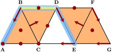
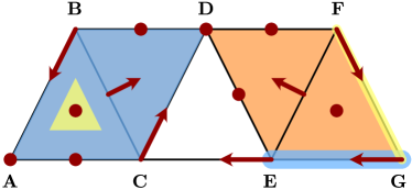
Figure 12. The combinatorial flow $\Phi$. The above two panels illustrate the action of the combinatorial flows associated with the two combinatorial vector fields introduced in the top two rows of Figure 6. In the left panel, both the chain $\mathbf{B}\mathbf{D}$ and its image $\Phi_{1}(\mathbf{B}\mathbf{D})$ are shown in yellow and blue, respectively. In the panel on the right one can find $\Phi_{2}(\mathbf{A}\mathbf{B}\mathbf{C})$ and $\Phi_{2}(\mathbf{F}\text{$\mathbf{G}$})$, where again the arguments are depicted in yellow and the images under the combinatorial flow in blue.

Example 8.5 (Three Forman gradient vector fields).

We return to the setting of Example 2.17, where we introduced the three combinatorial vector fields shown in Figure 6. For this, consider the underlying simplicial complex $X$ as a Lefschetz complex with $\mbox{$\mathbb{Z}$}_{2}$-coefficients, that is, the simplices making up the complex $X$ are not oriented.

In order to describe the action of the combinatorial flows $\Phi$ associated with the two gradient combinatorial vector fields shown in Figure 12, one first needs to understand the chain map $\Gamma$ defined in (104). It can easily be seen that due to the used $\mbox{$\mathbb{Z}$}_{2}$-coefficients, the image $\Gamma(x)$ is nonzero if and only if $x=x^{-}\neq x^{+}$, and in this case we have $\Gamma(x^{-})=x^{+}$.

With this, we can now turn our attention to a few sample combinatorial flow computations. We begin by considering the combinatorial vector field $\text{$\mathcal{V}$}_{1}$ shown in the left panel of Figure 12. For the edge $\mathbf{B}\mathbf{D}$ one obtains

$$\Phi_{1}(\mathbf{B}\mathbf{D}) = \mathbf{B}\mathbf{D}+\partial(\Gamma_{1}(\mathbf{B}\mathbf{D}))+\Gamma_{1}(\partial\mathbf{B}\mathbf{D})$$

$$= \mathbf{B}\mathbf{D}+\partial(0)+\Gamma_{1}(\mathbf{B}+\mathbf{D})\;\;=\;\;\mathbf{B}\mathbf{D}+\mathbf{A}\mathbf{B}+\mathbf{D}\mathbf{E},$$

and this is illustrated in the left image of Figure 12. The edge $\mathbf{B}\mathbf{D}$ is shown in yellow, while the chain $\Phi_{1}(\mathbf{B}\mathbf{D})$ is drawn in blue. Notice that the action of the combinatorial flow $\Phi_{1}$ encodes potential solution paths of the combinatorial vector field $\text{$\mathcal{V}$}_{1}$ starting at $\mathbf{B}\mathbf{D}$.

For the gradient combinatorial vector field $\text{$\mathcal{V}$}_{2}$ shown in the right panel of Figure 12 we consider two examples. First, the edge $\mathbf{F}\text{$\mathbf{G}$}$ has the image

$$\Phi_{2}(\mathbf{F}\text{$\mathbf{G}$})=\mathbf{F}\text{$\mathbf{G}$}+\partial(0)+\Gamma(\mathbf{F}+\text{$\mathbf{G}$})=\mathbf{F}\text{$\mathbf{G}$}+\mathbf{F}\text{$\mathbf{G}$}+\mathbf{E}\text{$\mathbf{G}$}=\mathbf{E}\text{$\mathbf{G}$},$$

since both $\Gamma(\mathbf{F}\text{$\mathbf{G}$})=0$ and $\mathbf{F}\text{$\mathbf{G}$}+\mathbf{F}\text{$\mathbf{G}$}=0$ are satisfied. In addition, for the two-dimensional cell $\mathbf{A}\mathbf{B}\mathbf{C}$ one obtains the identity

$$\Phi_{2}(\mathbf{A}\mathbf{B}\mathbf{C}) = \mathbf{A}\mathbf{B}\mathbf{C}+\partial(0)+\Gamma_{2}(\mathbf{A}\mathbf{B}+\mathbf{A}\mathbf{C}+\mathbf{B}\mathbf{C})$$

$$= \mathbf{A}\mathbf{B}\mathbf{C}+0+0+\mathbf{B}\mathbf{C}\mathbf{D}\;\;=\;\;\mathbf{A}\mathbf{B}\mathbf{C}+\mathbf{B}\mathbf{C}\mathbf{D},$$

in view of $\Gamma_{2}(\mathbf{A}\mathbf{B}\mathbf{C})=0$ and $\Gamma_{2}(\mathbf{A}\mathbf{B})=\Gamma_{2}(\mathbf{A}\mathbf{C})=0$, as well as using our above discussion to show that $\Gamma_{2}(\mathbf{B}\mathbf{C})=\mathbf{B}\mathbf{C}\mathbf{D}$. Both of these images under the combinatorial flow $\Phi_{2}$ are depicted in blue in the right panel of Figure 12, while the considered arguments are shown in yellow. $\Diamond$

The above sample computations demonstrate that the combinatorial flow in some sense encodes the potential paths that solutions of the combinatorial vector field can take. For later use, we now present four propositions, which provide more rigorous insight into the action of the combinatorial flow $\Phi$.

Proposition 8.6.

Suppose that $X$ is a regular Lefschetz complex and $\mathcal{V}$ is a combinatorial gradient vector field on $X$. Then for all $x\in X$ we have

$$\langle x,\Phi x\rangle=\begin{cases}1&\text{if $x\in X^{c}$,}\\ 0&\text{otherwise.}\end{cases}$$

Proof: We have $\langle x,\Phi x\rangle=\langle x,x\rangle+\langle x,{\bf\partial}\Gamma x\rangle+\langle x,\Gamma{\bf\partial}x\rangle$. In the case $x\in X^{c}$ we get from Proposition 8.4 that $\langle x,{\bf\partial}\Gamma x\rangle=0$ and $\langle x,\Gamma{\bf\partial}x\rangle=0$, which implies $\langle x,\Phi x\rangle=\langle x,x\rangle=1$.

Consider now the case $x\in X^{-}$. Then one has $x=x^{-}\not\in X^{+}$ and one obtains from (105) that $\langle x,\Gamma{\bf\partial}x\rangle=0$. Therefore, the definition (104) yields

$$\langle x,\Phi x\rangle=\langle x,x\rangle+\langle x,{\bf\partial}\Gamma x\rangle=\\ 1-\kappa(x^{+},x^{-})^{-1}\langle x,x^{-}\rangle\langle x,{\bf\partial}x^{+}\rangle=1-\kappa(x^{+},x^{-})^{-1}\kappa(x^{+},x^{-})=0.$$

Finally, we consider the remaining case $x\in X^{+}$. Then $x\not\in X^{-}$, and (106) shows that $\langle x,{\bf\partial}\Gamma x\rangle=0$ . Therefore, since ${\bf\partial}x=\sum_{y\in X}\kappa(x,y)y$, one has

$$\langle x,\Phi x\rangle=\langle x,x\rangle+\langle x,\Gamma{\bf\partial}x\rangle=1+\langle x,\sum_{y\in X}\kappa(x,y)\Gamma y\rangle\\ =1-\langle x,\sum_{y\in X,\;\Gamma y\neq 0}\kappa(x,y)\kappa(y^{+},y^{-})^{-1}\langle y,y^{-}\rangle y^{+}\rangle\\ =1-\sum_{y\in X,\;\Gamma y\neq 0}\kappa(x,y)\kappa(y^{+},y^{-})^{-1}\langle y,y^{-}\rangle\langle x,y^{+}\rangle\\ =1-\kappa(x^{+},x^{-})\kappa(x^{+},x^{-})^{-1}=0,$$

because the only non-zero term in the last sum occurs for the point $y\in X$ which satisfies both $y^{+}=x=x^{+}$ and $y=y^{-}=x^{-}$. ∎

Proposition 8.7.

Suppose that $X$ is a regular Lefschetz complex and $\mathcal{V}$ is a combinatorial gradient vector field on $X$. Then we have

$$\Phi(C(X^{+}))\subset C(X^{+}).$$

Proof: Since $\Phi$ is linear, it suffices to show that the inclusion $x\in X^{+}$ implies $|\Phi x|\subset X^{+}$. Thus, take $x\in X^{+}$ and a $u\in|\Phi x|$. Then $\langle u,\Phi x\rangle\neq 0$. From (106) we get $\langle u,{\bf\partial}\Gamma x\rangle=0$. Therefore, $0\neq\langle u,\Phi x\rangle=\langle u,x\rangle+\langle u,\Gamma{\bf\partial}x\rangle$, which implies $\langle u,x\rangle\neq 0$ or $\langle u,\Gamma{\bf\partial}x\rangle\neq 0$. If $\langle u,x\rangle\neq 0$, then $u=x\in X^{+}$. If the inequality $\langle u,\Gamma{\bf\partial}x\rangle\neq 0$ holds, then we get from (105) that $u\in X^{+}$. Hence, $|\Phi x|\subset X^{+}$. ∎

Proposition 8.8.

Suppose that $X$ is a regular Lefschetz complex and that $\mathcal{V}$ is a given combinatorial gradient vector field on $X$. Assume further that the inclusion $\text{$\mathcal{A}$}\in\mbox{$\operatorname{Down}$}(\text{$\mathcal{V}$},\leq_{\text{$\mathcal{V}$}})$ holds. Then $A:=|\text{$\mathcal{A}$}|$ is a $\mathcal{V}$-compatible and closed subset of $X$, and we have the inclusion $\Phi(C(A))\subset C(A)$. Therefore, the restriction $\Phi_{|C(A)}:(C(A),{\bf\partial}^{\kappa}_{|C(A)})\to(C(A),{\bf\partial}^{\kappa}_{|C(A)})$ is again a well-defined chain map.

Proof: Clearly, $A$ is $\mathcal{V}$-compatible, and it follows from Proposition 6.1(i) that $A$ is closed. Take an $x\in A$. We will prove that $\Phi x\in C(A)$. Since $A$ is closed, we have $|{\bf\partial}x|\subset A$. Since $A$ is $\mathcal{V}$-compatible, we have $|\Gamma_{\text{$\mathcal{V}$}}x|\subset A$. Thus, again by closedness and $\mathcal{V}$-compatibility of $A$, we get both $|{\bf\partial}\Gamma_{\text{$\mathcal{V}$}}x|\subset A$ and $|\Gamma_{\text{$\mathcal{V}$}}{\bf\partial}x|\subset A$. Therefore,

$$|\Phi x|=|x+{\bf\partial}\Gamma_{\text{$\mathcal{V}$}}x+\Gamma_{\text{$\mathcal{V}$}}{\bf\partial}x|\subset|x|\cup|{\bf\partial}\Gamma_{\text{$\mathcal{V}$}}x|\cup|\Gamma_{\text{$\mathcal{V}$}}{\bf\partial}x|\subset A.$$

This finally implies $\Phi x\in C(A)$ and completes the proof. ∎

Proposition 8.9.

Suppose that $X$ is a regular Lefschetz complex and $\mathcal{V}$ is a combinatorial gradient vector field on $X$. Assume further that $x,y\in X$. Then the following hold:

• If $y\in|\Phi x|$, then $[y]\leq_{\text{$\mathcal{V}$}}[x]$, and there exists a path from $x$ to $y$ with respect to the multivalued flow map $\Pi_{\text{$\mathcal{V}$}}$ defined in (86).

• If $y\in|\Phi x|$ and $[y]=[x]$, then $y=x$ .

• If $x\in|\Phi x|$, then $\langle x,\Phi x\rangle=1$.

In addition, for any chain $c\in C(X)$ the following holds:

• If $c=\Phi(c)$ and $c\neq 0$, then $|c|$ has to contain a critical cell.

Proof: In order to see (i), observe that the assumption $y\in|\Phi x|$ implies the inequality $0\neq\langle y,\Phi x\rangle=\langle y,x\rangle+\langle y,{\bf\partial}\Gamma x\rangle+\langle y,\Gamma{\bf\partial}x\rangle$. Thus, either we have $\langle y,x\rangle\neq 0$, or $\langle y,{\bf\partial}\Gamma x\rangle\neq 0$, or $\langle y,\Gamma{\bf\partial}x\rangle\neq 0$. In the first case one immediately obtains $x=y$ and $[x]=[y]$. Consider now the second case $\langle y,{\bf\partial}\Gamma x\rangle\neq 0$. This inequality yields both $\Gamma x\neq 0$ and $y\in|{\bf\partial}\Gamma x|$. Hence, we have $x=x^{-}$ and $\Gamma x=\lambda x^{+}$ with $\lambda=-\kappa(x^{+},x^{-})^{-1}\neq 0$. This gives $|{\bf\partial}\Gamma x|=|{\bf\partial}x^{+}|$, as well as $y\in|{\bf\partial}x^{+}|\subset\operatorname{cl}x^{+}$. It follows that $y\in[y]\cap\operatorname{cl}[x^{+}]=[y]\cap\operatorname{cl}[x^{-}]$, and therefore $[y]\leq_{\text{$\mathcal{V}$}}[x]$. Finally, we consider the third inequality $\langle y,\Gamma{\bf\partial}x\rangle\neq 0$. Since ${\bf\partial}x=\sum_{u\in X}\kappa(x,u)u$, we have

$$0\neq\langle y,\Gamma{\bf\partial}x\rangle=\sum_{u\in X}\kappa(x,u)\langle y,\Gamma u\rangle,$$

which implies $\langle y,\Gamma u\rangle\neq 0$ for some $u\in|{\bf\partial}x|$. But this implies that $u=u^{-}$ and $\Gamma u=\lambda u^{+}$ with $\lambda=-\kappa(u^{+},u^{-})^{-1}\neq 0$. Hence, the identities $y=u^{+}$ and $[y]=[u^{+}]=[u^{-}]$ are satisfied, as well as the inclusion $u^{-}\in|{\bf\partial}x|\subset\operatorname{cl}x$. Thus, $[y]\cap\operatorname{cl}[x]\neq\varnothing$, which implies $[y]\leq_{\text{$\mathcal{V}$}}[x]$. Furthermore, in all of these three cases one can easily construct a path from $x$ to $y$ with respect to the multivalued map $\Pi_{\text{$\mathcal{V}$}}$. This finally completes the proof of (i).

In order to prove (ii), we observe that $y\in|\Phi x|$ implies $\dim x=\dim y$, since $\Phi$ is a degree zero module homomorphism. Since $\mathcal{V}$ is a combinatorial vector field, we further have both $[x]=\{x^{-},x^{+}\}$ and $[y]=\{y^{-},y^{+}\}$. Thus, the validity of $[x]=[y]$ and $y\in|\Phi x|$ implies the identity $x=y$, which in turn establishes (ii).

We now turn our attention to (iii). If $x\in|\Phi x|$, then $\langle x,\Phi x\rangle\neq 0$. Thus, we get from Proposition 8.6 that $\langle x,\Phi x\rangle=1$.

Finally, consider (iv). Let $y\in|c|$ be such that $[y]$ is a maximal element with respect to $\leq_{\text{$\mathcal{V}$}}$. In other words, there is no $z\in|c|$ for which $[y]<_{\text{$\mathcal{V}$}}[z]$. Since

$$y\in|c|=|\Phi(c)|\subset\bigcup_{x\in|c|}|\Phi(x)|,$$

there exists an $x\in|c|$ with $y\in|\Phi(x)|$. Then part (i) implies $[y]\leq_{\text{$\mathcal{V}$}}[x]$, and in view of our choice of $y$ this yields $[y]=[x]$. But then (ii) furnishes $y=x$, and an application of (iii) gives $\langle x,\Phi x\rangle=1$. Together with Proposition 8.6 one finally obtains $y=x\in X^{c}$ as claimed. ∎

8.2. The stabilized combinatorial flow

As mentioned earlier, the combinatorial flow describes on the level of chains the possible future evolutions of solutions of the underlying combinatorial vector field. Thus, in the case of combinatorial gradient vector fields iterations of $\Phi$ should eventually stabilize and provide intuition on potential connecting orbits between critical cells. In other words, such a stabilization of the combinatorial flow should encode both the Conley complex and the associated connection matrix.

However, before we can show that such a stabilization exists, we first have to study the behavior of iterates of the combinatorial flow. We begin with a result which is an easy application of Proposition 8.9 and shows that cells in $|\Phi^{n}x|$ have to belong to vectors below $[x]$ in the partial order $\leq_{\text{$\mathcal{V}$}}$, regardless of the iteration number $n\in\mbox{$\mathbb{N}$}$.

Proposition 8.10.

Assume that $\mathcal{V}$ is a combinatorial gradient vector field on a regular Lefschetz complex $X$. If $y\in|\Phi^{n}x|$ for some $n\in\mbox{$\mathbb{N}$}$, then the inequality $[y]\leq_{\text{$\mathcal{V}$}}[x]$ is satisfied.

Proof: We proceed by induction on $n$. For $n=1$ the conclusion is the statement of Proposition 8.9. Thus, fix an $n\in\mbox{$\mathbb{N}$}$ and assume that the conclusion holds for all $k\in\{1,2,\ldots n\}$. Let $y\in|\Phi^{n+1}x|$ and let $c:=\Phi^{n}x$. Then $c=\sum_{w\in|c|}\langle c,w\rangle w$ and $\Phi c=\sum_{w\in|c|}\langle c,w\rangle\Phi w$. Since

$$y\in|\Phi^{n+1}x|=|\Phi c|\subset\bigcup_{w\in|c|}|\Phi w|,$$

we get $y\in|\Phi w|$ for some $w\in|c|=|\Phi^{n}x|$. Thus, by our induction assumption, we obtain $[y]\leq_{\text{$\mathcal{V}$}}[w]\leq_{\text{$\mathcal{V}$}}[x]$. ∎

Next, we study in more detail the specific form of the image chain $\Phi^{n}x$ if the cell $x$ is a critical cell and $n\in\mbox{$\mathbb{N}$}$. This result will prove to be essential for identifying the Conley complex associated with $\mathcal{V}$.

Proposition 8.11.

Assume that $\mathcal{V}$ is a combinatorial gradient vector field on a regular Lefschetz complex $X$. Then for every critical cell $x\in X^{c}$ and every positive integer $n\in\mbox{$\mathbb{N}$}$ we have the representation

(108) $$\Phi^{n}x=x+r_{x,n}$$

where $r_{x,n}$ is a chain satisfying

(109) $$|r_{x,n}|\subset X^{+}\cap|\,[x]^{<_{\text{$\mathcal{V}$}}}\,|.$$

Proof: We proceed by induction on $n$. Assume first that one has $n=1$ and set $r_{x,1}:=\Gamma{\bf\partial}x$. From Proposition 8.3 we see that $|r_{x,1}|\subset X^{+}$ and, since we assumed $x\in X^{c}$, one obtains further $\langle x,r_{x,1}\rangle=0$. The inclusion $x\in X^{c}$ also shows that $\Gamma x=0$, and therefore the identity $\Phi x=x+\Gamma{\bf\partial}x=x+r_{x,1}$ holds. To show that $|r_{x,1}|\subset|\,[x]^{<_{\text{$\mathcal{V}$}}}\,|$, take an arbitrary $y\in|r_{x,1}|$. Then we have $\langle y,r_{x,1}\rangle\neq 0$, and since $\langle x,r_{x,1}\rangle=0$, we get $x\neq y$, that is, $\langle y,x\rangle=0$. It follows that $\langle y,\Phi x\rangle=\langle y,x\rangle+\langle y,r_{x,1}\rangle=\langle y,r_{x,1}\rangle\neq 0$. Hence, $y\in|\Phi x|$. Thus, Proposition 8.9(i) gives $[y]\leq_{\text{$\mathcal{V}$}}[x]$ and $[y]\in[x]^{\leq_{\text{$\mathcal{V}$}}}$. Since $y\neq x$, and in view of the fact that $\Phi$ is a degree $0$ map, one further has $\dim y=\dim x$, and we also get $[y]\neq[x]$ and $[y]\in[x]^{<_{\text{$\mathcal{V}$}}}$. This in turn yields $y\in|\,[x]^{<_{\text{$\mathcal{V}$}}}\,|$. Therefore, $|r_{x,1}|\subset|\,[x]^{<_{\text{$\mathcal{V}$}}}\,|$, and the proof of (108) for $n=1$ is complete.

Next, fix a $k\in\mbox{$\mathbb{N}$}$ and assume that (108) holds for all $n\leq k$ with $r_{x,n}$ satisfying (109). Then $\Phi^{k+1}x=\Phi(\Phi^{k}x)=\Phi x+\Phi r_{x,k}=x+r_{x,1}+\Phi r_{x,k}$, and we set $r_{x,k+1}:=r_{x,1}+\Phi r_{x,k}$. It follows from the induction assumption and Proposition 8.7 that $|r_{x,k+1}|\subset|r_{x,1}|\cup|\Phi r_{x,k}|\subset X^{+}$. Since $|r_{x,1}|\subset|\,[x]^{<_{\text{$\mathcal{V}$}}}\,|$, it suffices to prove that $|\Phi r_{x,k}|\subset|\,[x]^{<_{\text{$\mathcal{V}$}}}\,|$ in order to see that $|r_{x,k+1}|\subset|\,[x]^{<_{\text{$\mathcal{V}$}}}\,|$. For this, take an arbitrary element $y\in|r_{x,k}|$. Then the induction assumption gives $y\in|\,[x]^{<_{\text{$\mathcal{V}$}}}\,|$. Since $|\,[x]^{<_{\text{$\mathcal{V}$}}}\,|$ is $\mathcal{V}$-compatible, it follows that $[y]\in[x]^{<_{\text{$\mathcal{V}$}}}$. Since $[x]^{<_{\text{$\mathcal{V}$}}}$ is a down set, we get $[y]^{\leq_{\text{$\mathcal{V}$}}}\subset[x]^{<_{\text{$\mathcal{V}$}}}$ and $|\,[y]^{\leq_{\text{$\mathcal{V}$}}}\,|\subset|\,[x]^{<_{\text{$\mathcal{V}$}}}\,|$. Thus, we proved that

(110) $$y\in|r_{x,k}|\quad\;\Rightarrow\;\quad|\,[y]^{\leq_{\text{$\mathcal{V}$}}}\,|\subset|\,[x]^{<_{\text{$\mathcal{V}$}}}\,|.$$

We have $r_{x,k}=\sum_{y\in|r_{x,k}|}\langle r_{x,k},y\rangle y$ and $\Phi r_{x,k}=\sum_{y\in|r_{x,k}|}\langle r_{x,k},y\rangle\Phi y$. In view of Proposition 8.9(i) and property (110) one then obtains the inclusion

$$|\Phi r_{x,k}|\subset\bigcup_{y\in|r_{x,k}|}|\Phi y|\subset\bigcup_{y\in|r_{x,k}|}|\,[y]^{\leq_{\text{$\mathcal{V}$}}}|\,\subset|\,[x]^{<_{\text{$\mathcal{V}$}}}\,|,$$

which completes the induction argument, and therefore the proof. ∎

The statement of the above proposition can be illustrated using the sample computations in Example 8.5, two of which have arguments which are critical cells. As shown in the left panel of Figure 12, for the gradient combinatorial vector field $\text{$\mathcal{V}$}_{1}$ one has the identity $\Phi_{1}(\mathbf{B}\mathbf{D})=\mathbf{B}\mathbf{D}+\mathbf{A}\mathbf{B}+\mathbf{D}\mathbf{E}$, i.e., in this situation $r_{\mathbf{B}\mathbf{D},1}=\mathbf{A}\mathbf{B}+\mathbf{D}\mathbf{E}$. Similarly, for the vector field $\text{$\mathcal{V}$}_{2}$ in the right panel one has $\Phi_{2}(\mathbf{A}\mathbf{B}\mathbf{C})=\mathbf{A}\mathbf{B}\mathbf{C}+\mathbf{B}\mathbf{C}\mathbf{D}$, which leads to $r_{\mathbf{A}\mathbf{B}\mathbf{C},1}=\mathbf{B}\mathbf{C}\mathbf{D}$. In both cases, the chain $r_{x,1}$ clearly satisfies (109).

After these preparations we can finally show that iterations of the combinatorial flow have to stabilize. In the context of the Morse complex this was already shown by Forman in [12]. The following result is modeled after [12, Theorem 7.2], yet adapted to our situation.

Proposition 8.12.

Assume again that $\mathcal{V}$ denotes a combinatorial gradient vector field on a regular Lefschetz complex $X$, and consider the combinatorial flow $\Phi=\Phi_{\text{$\mathcal{V}$}}:C(X)\to C(X)$ defined in (107). In this case there exists an integer $N\in\mbox{$\mathbb{N}$}$ such that

$$\Phi^{n}=\Phi^{N}\quad\mbox{ for all }\quad n\geq N.$$

We then define $\Phi^{\infty}:=\Phi^{N}$ and call it the stabilized combinatorial flow.

Proof: We show that for every $x\in X$ there exists an integer $n_{x}\in\mbox{$\mathbb{N}$}$ such that $\Phi^{n_{x}+1}x=\Phi^{n_{x}}x$ holds. Then it is straightforward to see that choosing $N$ as the maximum of $\{n_{x}\mid x\in X\}$ satisfies the statement of the proposition.

In order to prove the above claim, we proceed by induction over the number of vectors which are strictly below $[x]$ with respect to $<_{\text{$\mathcal{V}$}}$, that is, by induction over the number

$$L(x):=\#\{V\in\text{$\mathcal{V}$}\,\mid\,V<_{\text{$\mathcal{V}$}}[x]\}.$$

Suppose first that $x\in X$ is such that $L(x)=0$. If we have $\Phi x=0$, then clearly $\Phi^{2}x=\Phi x=0$ and the statement follows. Otherwise there exists a cell $y\in X$ with $y\in|\Phi x|$. But then Proposition 8.9(i) implies $[y]\leq_{\text{$\mathcal{V}$}}[x]$, and the identity $L(x)=0$ further yields $[y]=[x]$. This in turn gives both $y=x$ and $x\in|\Phi x|$, as well as $\langle x,\Phi x\rangle=1$, in view of Proposition 8.9(ii),(iii). In other words, we have to have $\Phi x=x$, and the claim follows again.

Now let $k\in\mbox{$\mathbb{N}$}$ be arbitrary and assume that we have verified the claim for all $z\in X$ with $L(z)<k$. Moreover, let $x\in X$ be a cell with $L(x)=k$. We now distinguish the cases of $x$ being critical or not.

Assume first that $x$ is not a critical cell. Then for all $y\in|\Phi x|$ one has to have $[y]<_{\text{$\mathcal{V}$}}[x]$. To show this, suppose otherwise that there is a $y\in|\Phi x|$ with $[y]=[x]$. Then Proposition 8.9(ii),(iii) implies $y=x$ and $\langle x,\Phi x\rangle=1$, and in view of Proposition 8.6 this gives $x\in X^{c}$, a contradiction. Together with Proposition 8.9(i), we therefore have $[y]<_{\text{$\mathcal{V}$}}[x]$ for all $y\in|\Phi x|$ as claimed. Thus, every term in the representation

$$\Phi x=\sum_{y\in|\Phi x|}\langle y,\Phi x\rangle y$$

satisfies $L(y)<k$, and according to the inductive hypothesis there exists, after possibly taking the maximum of the individual values, an $m\in\mbox{$\mathbb{N}$}$ such that $\Phi^{m+1}y=\Phi^{m}y$ for all $y\in|\Phi x|$. This finally furnishes

$$\Phi^{m+2}x=\sum_{y\in|\Phi x|}\langle y,\Phi x\rangle\Phi^{m+1}y=\sum_{y\in|\Phi x|}\langle y,\Phi x\rangle\Phi^{m}y=\Phi^{m+1}x,$$

and the claim from the beginning of the proof follows for non-critical $x$.

Finally, suppose that $x\in X^{c}$. According to Proposition 8.11 there exists a chain $r_{x,1}$ satisfying (109) as well as $\Phi x=x+r_{x,1}$. A straightforward induction argument then implies

$$\Phi^{\ell}x=x+r_{x,1}+\Phi r_{x,1}+\ldots+\Phi^{\ell-1}r_{x,1}\quad\mbox{ for all }\quad\ell\in\mbox{$\mathbb{N}$}.$$

Thus, in order to establish that one has $\Phi^{m+1}x=\Phi^{m}x$ for some $m\in\mbox{$\mathbb{N}$}$ it suffices to show that $\Phi^{m}r_{x,1}=0$. Notice that according to (109) we can apply the inductive hypothesis to $r_{x,1}$, and therefore there exists an integer $m\in\mbox{$\mathbb{N}$}$ such that $\Phi^{m+1}r_{x,1}=\Phi^{m}r_{x,1}$. This immediately shows that $\Phi^{m}r_{x,1}$ is a fixed chain under the combinatorial flow $\Phi$. Furthermore, the inclusion in (109) and Proposition 8.7 yield $|\Phi^{m}r_{x,1}|\subset X^{+}$. But then Proposition 8.9(iv) implies that we have to have $\Phi^{m}r_{x,1}=0$, since the support of $\Phi^{m}r_{x,1}$ contains no critical cells. This finally establishes the induction step also for a critical cell $x$, and the proof is complete. ∎

We would like to point out that in view of this result, the stabilized combinatorial flow $\Phi^{\infty}$ also satisfies the statements in Propositions 8.10 and 8.11, as long as we replace $n$ by $\infty$ in their formulations.

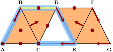
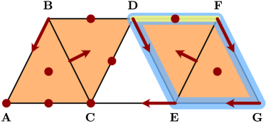
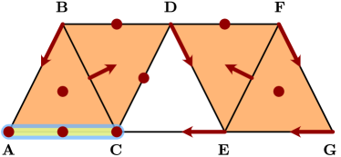
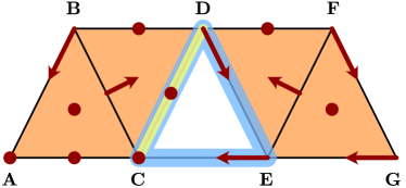
Figure 13. The stabilized combinatorial flow. For the gradient combinatorial vector field $\text{$\mathcal{V}$}_{1}$ introduced in the first row of Figure 6, the four panels show the images $\Phi_{1}^{\infty}(x)$ for the one-dimensional critical cells $x$. From top left to bottom right the panels depict the chains $\Phi_{1}^{\infty}(\mathbf{B}\mathbf{D})$, $\Phi_{1}^{\infty}(\mathbf{D}\mathbf{F})$, $\Phi_{1}^{\infty}(\mathbf{A}\mathbf{C})$, and $\Phi_{1}^{\infty}(\mathbf{C}\mathbf{D})$, respectively, in blue.

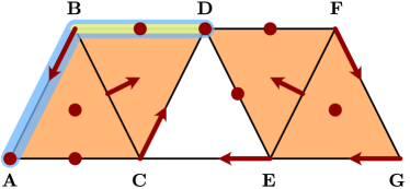
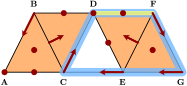
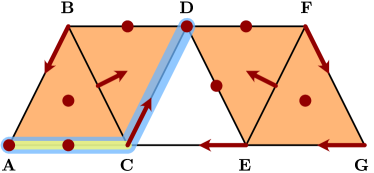
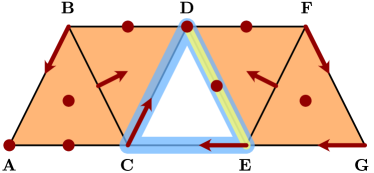
Figure 14. The stabilized combinatorial flow. For the gradient vector field $\text{$\mathcal{V}$}_{2}$ introduced in the second row of Figure 6, the above four panels show the images $\Phi_{2}^{\infty}(x)$ for the one-dimensional critical cells $x$. From top left to bottom right they depict the chains $\Phi_{2}^{\infty}(\mathbf{B}\mathbf{D})$, $\Phi_{2}^{\infty}(\mathbf{D}\mathbf{F})$, $\Phi_{2}^{\infty}(\mathbf{A}\mathbf{C})$, and $\Phi_{2}^{\infty}(\mathbf{D}\mathbf{E})$, respectively, in blue.

Example 8.13 (Three Forman gradient vector fields).

To illustrate the action of the stabilized flow, we return to Examples 2.17 and 8.5. For the two gradient combinatorial vector fields $\text{$\mathcal{V}$}_{1}$ and $\text{$\mathcal{V}$}_{2}$ shown in the first two rows of Figure 6, and in Figure 12, what are the images of the critical cells under the stabilized combinatorial flow?

We begin by considering the zero-dimensional critical cells in the vector fields. Clearly, both their boundaries and images under $\Gamma$ are trivial, and therefore we have $\Phi_{k}^{\infty}(x)=x$ for all of these cells. In addition, for the two-dimensional cells one easily obtains that $\Phi_{k}^{\infty}(\mathbf{A}\mathbf{B}\mathbf{C})=\mathbf{A}\mathbf{B}\mathbf{C}+\mathbf{B}\mathbf{C}\mathbf{D}$, as well as $\Phi_{k}^{\infty}(\mathbf{E}\mathbf{F}\text{$\mathbf{G}$})=\mathbf{E}\mathbf{F}\text{$\mathbf{G}$}+\mathbf{D}\mathbf{E}\mathbf{F}$. This follows easily from the computation in Example 8.5, together with the fact that $\Phi_{k}(\mathbf{B}\mathbf{C}\mathbf{D})=\Phi_{k}(\mathbf{D}\mathbf{E}\mathbf{F})=0$, which in turn implies that the second iterate of $\Phi_{k}$ coincides with the first iterate on critical cells of dimension two.

This leaves us with the one-dimensional critical cells. As it turns out, their images under the stabilized flow can be different with respect to $\text{$\mathcal{V}$}_{1}$ or $\text{$\mathcal{V}$}_{2}$. The resulting images $\Phi_{k}^{\infty}(x)$ are shown in Figure 13 for $k=1$, and in Figure 14 for $k=2$. Notice that in almost all of these cases, the image of a one-dimensional cell $x$ under the stabilized flow is given by the support of all connecting orbits between the cell $x$ and zero-dimensional critical cells. The only exception is the image $\Phi_{1}^{\infty}(\mathbf{D}\mathbf{F})$, which lacks the edge $\mathbf{C}\mathbf{E}$. Yet, since this edge is contained in both connecting orbits between $\mathbf{D}\mathbf{F}$ and $\mathbf{C}$, the sum of the associated two chains with respect to $\mbox{$\mathbb{Z}$}_{2}$-coefficients leads to its cancellation. $\Diamond$

The stabilized combinatorial flow is our main tool for the construction of the Conley complex and its associated connection matrix for a combinatorial gradient vector field $\mathcal{V}$ on a regular Lefschetz complex $X$. It follows immediately from Proposition 8.12 that for every chain $c\in C(X)$ we have

$$\Phi(\Phi^{\infty}(c))=\Phi(\Phi^{n}(c))=\Phi^{n+1}(c)=\Phi^{\infty}(c),$$

that is, the image $\Phi^{\infty}(c)$ is a fixed point of the combinatorial flow $\Phi$. We therefore consider the set

(111) $$\operatorname{Fix}\Phi:=\mbox{$\{\,c\in C(X)\mid\Phi c=c\,\}$}$$

consisting of chains fixed by $\Phi$. Clearly, if $c\in\operatorname{Fix}\Phi$, then ${\bf\partial}c\in\operatorname{Fix}\Phi$, because $\Phi{\bf\partial}c={\bf\partial}\Phi c={\bf\partial}c$. It follows that $(\operatorname{Fix}\Phi,{\bf\partial}_{|\operatorname{Fix}\Phi})$ is a chain subcomplex of $(C(X),{\bf\partial})$. Furthermore, since $\Phi$ is a chain map, Proposition 8.12 further implies that $\Phi^{\infty}:(C(X),{\bf\partial})\to(\operatorname{Fix}\Phi,{\bf\partial}_{|\operatorname{Fix}\Phi})$ is a chain map as well. Yet even more is true, as the following result demonstrates.

Proposition 8.14.

Assume that $\mathcal{V}$ is a combinatorial gradient vector field on a regular Lefschetz complex $X$, and let $\Phi^{\infty}$ denote the associated stabilized combinatorial flow. Then the restriction $\Phi^{\infty}_{|C(X^{c})}:C(X^{c})\to\operatorname{Fix}\Phi$ is an isomorphism. Moreover, if we define the projection $\Pi:\operatorname{Fix}\Phi\to C(X^{c})$ via

(112) $$\Pi c:=\sum_{x\in X^{c}}\langle c,x\rangle x\quad\mbox{ for every }\quad c\in\operatorname{Fix}\Phi,$$

then we have $\Phi^{\infty}\Pi c=c$ for all $c\in\operatorname{Fix}\Phi$.

Proof: We begin by verifying that $\Phi^{\infty}_{|C(X^{c})}$ is a monomorphism. For this, suppose that $c\in C(X^{c})$ is a chain with $\Phi^{\infty}c=0$. Then $c=\sum_{x\in X^{c}}a_{x}x$, and the representation in (108) further yields

$$0=\Phi^{\infty}c=\sum_{x\in X^{c}}a_{x}\Phi^{\infty}x=c+\sum_{x\in X^{c}}a_{x}r_{x}\in C(X^{c})\oplus C(X^{+}).$$

Hence, it follows that $c=0$, and therefore $\Phi^{\infty}_{|C(X^{c})}$ is one-to-one.

In order to prove that $\Phi^{\infty}_{|C(X^{c})}:C(X^{c})\to\operatorname{Fix}\Phi$ is onto, let $c\in\operatorname{Fix}\Phi$ be arbitrary and consider the chain $\Pi c\in C(X^{c})$ defined in (112). Then we have

$$\Phi^{\infty}\Pi c=\sum_{x\in X^{c}}\langle c,x\rangle\Phi^{\infty}x,$$

and for every critical cell $y\in X^{c}$ the representation of $\Phi^{\infty}x$ in Proposition 8.11 further implies $\langle\Phi^{\infty}x,y\rangle=\langle x+r_{x},y\rangle=\langle x,y\rangle$, see also (108). Thus one obtains

$$\langle\Phi^{\infty}\Pi c,y\rangle=\sum_{x\in X^{c}}\langle c,x\rangle\langle x,y\rangle=\langle c,y\rangle\quad\Rightarrow\quad\langle c-\Phi^{\infty}\Pi c,y\rangle=0$$

for all $y\in X^{c}$. In other words, the support of the chain $c-\Phi^{\infty}\Pi c$ does not contain a critical cell. In view of Proposition 8.9(iv) and $c-\Phi^{\infty}\Pi c\in\operatorname{Fix}\Phi$ this implies $c=\Phi^{\infty}\Pi c$, and thereby completes the proof of the result. ∎

The above result shows that the fixed chains under the combinatorial flow $\Phi$ are in one-to-one correspondence with chains of critical cells in the Lefschetz complex $X$. As the following result demonstrates, this fact can be used to both find a suitable basis of $\operatorname{Fix}\Phi$ which is indexed by the critical cells of $X$, as well as equip this basis with the structure of a Lefschetz complex.

Proposition 8.15.

Assume that $\mathcal{V}$ is a combinatorial gradient vector field on a regular Lefschetz complex $X$, and recall that $X^{c}\subset X$ denotes the set of all critical cells of $\mathcal{V}$. For every $x\in X^{c}$ set

$$\bar{x}:=\Phi^{\infty}x\in\operatorname{Fix}\Phi.$$

Then the following statements hold:

• The set $\bar{X}:=\mbox{$\{\,\bar{x}\mid x\in X^{c}\,\}$}$ is a basis of $\operatorname{Fix}\Phi$.

• For every $x\in X^{c}$ we have the representation

  (113) $${\bf\partial}\bar{x}=\sum_{z\in X^{c}}a_{xz}\bar{z},$$

  for uniquely determined coefficients $a_{xz}\in R$.

• The pair $(\bar{X},\bar{\kappa})$, where the $\mathbb{Z}$-gradation on $\bar{X}$ is induced by the map $\dim:\bar{X}\ni\bar{x}\mapsto\dim x\in\mbox{$\mathbb{Z}$}$, and where $\bar{\kappa}(\bar{x},\bar{z})$ is the coefficient $a_{xz}$ in (113), is a Lefschetz complex with $C(\bar{X})=\operatorname{Fix}\Phi$.

Proof: In order to prove (i), consider the projection $\Pi:\operatorname{Fix}\Phi\to C(X^{c})$ defined in Proposition 8.14, which has been shown to satisfy $\Phi^{\infty}\Pi=\operatorname{id}_{\operatorname{Fix}\Phi}$. In addition, let $c\in\operatorname{Fix}\Phi$ be arbitrary. Then one has

$$c=\Phi^{\infty}\Pi c=\Phi^{\infty}\sum_{x\in X^{c}}\langle c,x\rangle x=\sum_{x\in X^{c}}\langle c,x\rangle\Phi^{\infty}x=\sum_{x\in X^{c}}\langle c,x\rangle\bar{x},$$

which proves that $\bar{X}$ generates $\operatorname{Fix}\Phi$. To see that $\bar{X}$ is linearly independent, assume that

$$\sum_{x\in X^{c}}\alpha_{x}\bar{x}=0$$

for some coefficients $\alpha_{x}\in R$. Then $0=\sum_{x\in X^{c}}\alpha_{x}\Phi^{\infty}x=\Phi^{\infty}\sum_{x\in X^{c}}\alpha_{x}x$. Since $\sum_{x\in X^{c}}\alpha_{x}x\in C(X^{c})$, and $\Phi_{|C(X^{c})}:C(X^{c})\to\operatorname{Fix}\Phi$ is an isomorphism due to Proposition 8.14, we conclude that $\sum_{x\in X^{c}}\alpha_{x}x=0$. This in turn implies $\alpha_{x}=0$ for all $x\in X^{c}$. Thus, the set $\bar{X}$ is indeed a basis for $\operatorname{Fix}\Phi$.

In order to see (ii), we observe that ${\bf\partial}\bar{x}\in\operatorname{Fix}\Phi$, since $\Phi$ is a chain map. Thus, the representation in (113) is an immediate consequence of (i). Finally, a direct application of Proposition 3.14 shows that the pair $(\bar{X},\bar{\kappa})$ is a Lefschetz complex, and clearly $C(\bar{X})=\operatorname{Fix}\Phi$, which proves (iii). ∎

The Lefschetz complex $(\bar{X},\bar{\kappa})$ will take the role of the Conley complex associated with the combinatorial gradient vector field $\mathcal{V}$. For this, and as a last step, it is necessary to identify a natural partial order on its cells. This can be accomplished as follows.

Recall that $\mathcal{C}$ denotes the collection of all critical cells of $\mathcal{V}$. Then it follows easily from Proposition 8.11 that the map $X^{c}\ni x\mapsto\bar{x}\in\bar{X}$ is a bijection. Hence, also the map $\text{$\mathcal{C}$}\ni\{x\}\mapsto\bar{x}\in\bar{X}$ is a bijection, and this enables us to carry over the partial order $\leq_{\text{$\mathcal{V}$}}$ from $\text{$\mathcal{C}$}\subset\text{$\mathcal{V}$}$ to $\bar{X}$. Thus, for arbitrary elements $\bar{x},\bar{y}\in\bar{X}$ we write $\bar{x}\leq_{\text{$\mathcal{V}$}}\bar{y}$ if $\{x\}\leq_{\text{$\mathcal{V}$}}\{y\}$. Then we have the following result.

Proposition 8.16.

Assume that $\mathcal{V}$ is a combinatorial gradient vector field on a regular Lefschetz complex $X$. Then the above-defined partial order $\leq_{\text{$\mathcal{V}$}}$ in $\bar{X}$ is a natural partial order on the Lefschetz complex $(\bar{X},\bar{\kappa})$.

Proof: We begin by proving that the order $\leq_{\text{$\mathcal{V}$}}$ in $\bar{X}$ is admissible, that is, the validity of $\bar{y}\leq_{\bar{\kappa}}\bar{x}$ for $x,y\in X^{c}$ implies $\bar{y}\leq_{\text{$\mathcal{V}$}}\bar{x}$. Since the partial order $\leq_{\bar{\kappa}}$ is the transitive closure of $\prec_{\bar{\kappa}}$, it clearly suffices to prove that $\bar{y}\prec_{\bar{\kappa}}\bar{x}$ implies $\bar{y}\leq_{\text{$\mathcal{V}$}}\bar{x}$. Thus, assume that $x,y\in X^{c}$ and $\bar{y}\prec_{\bar{\kappa}}\bar{x}$. Then, $\bar{\kappa}(\bar{x},\bar{y})\neq 0$. By Proposition 8.15 we have ${\bf\partial}\bar{x}=\sum_{z\in X^{c}}a_{xz}\bar{z}$, with $a_{xz}=\bar{\kappa}(\bar{x},\bar{z})$. In addition, Propositions 8.11 and 8.12 imply $\bar{z}=\Phi^{\infty}z=z+r_{z,\infty}$, together with the inclusion $|r_{z,\infty}|\subset X^{+}\cap|\,[z]^{<_{\text{$\mathcal{V}$}}}\,|$. Since $y\in X^{c}\subset X\setminus X^{+}$, one further has

$$\langle{\bf\partial}\bar{x},y\rangle=\sum_{z\in X^{c}}a_{xz}\langle\bar{z},y\rangle=\sum_{z\in X^{c}}a_{xz}\left(\langle z,y\rangle+\langle r_{z,\infty},y\rangle\right)\\ =\sum_{z\in X^{c}}a_{xz}\langle z,y\rangle=a_{xy}=\bar{\kappa}(\bar{x},\bar{y})\neq 0.$$

It follows that

$$y\in|{\bf\partial}\bar{x}|=|{\bf\partial}\Phi^{\infty}x|=|\Phi^{\infty}{\bf\partial}x|=\left|\Phi^{\infty}\sum_{w\in|{\bf\partial}x|}\kappa(x,w)w\right|\subset\bigcup_{w\in|{\bf\partial}x|}|\Phi^{\infty}w|.$$

Thus, $y\in|\Phi^{\infty}u|$ for some $u\in X$ such that $\kappa(x,u)\neq 0$. From Proposition 8.10 we get $[y]\leq_{\text{$\mathcal{V}$}}[u]$. Since $\kappa(x,u)\neq 0$ we further have $u\in\operatorname{cl}x$, which in turn implies $u\in[u]\cap\operatorname{cl}[x]$. In consequence $[u]\leq_{\text{$\mathcal{V}$}}[x]$ and $\{y\}=[y]\leq_{\text{$\mathcal{V}$}}[x]=\{x\}$. Thus, by the definition of $\leq_{\text{$\mathcal{V}$}}$ in $\bar{X}$ we get $\bar{y}\leq_{\text{$\mathcal{V}$}}\bar{x}$.

To see that $\leq_{\text{$\mathcal{V}$}}$ is natural, we need to verify the implication in (74). Thus, let $\bar{x},\bar{y}\in\bar{X}$ satisfy both the inequality $\bar{x}\leq_{\text{$\mathcal{V}$}}\bar{y}$ and $\dim\bar{x}=\dim\bar{y}$. Then both $\{x\}\leq_{\text{$\mathcal{V}$}}\{y\}$ and $\dim x=\dim y$ hold as well. Yet this implies that one cannot have $\{x\}<_{\text{$\mathcal{V}$}}\{y\}$, because in this case, in view of Proposition 8.2(ii), one deduces the strict inequality $\dim x=\dim\{x\}<\dim\{y\}=\dim y$. It follows that $\{x\}=\{y\}$ and $\bar{x}=\bar{y}$, which proves that the order is natural. ∎

In the remaining last subsection of the paper, we consider $\bar{X}$ as a poset ordered by the natural partial order $\leq_{\text{$\mathcal{V}$}}$ in $\mathcal{V}$, which has been transferred to $\bar{X}$ via the map $\{x\}\mapsto\bar{x}$. In addition, the triple $(\bar{X},C(\bar{X}),{\bf\partial}^{\bar{\kappa}})$ is considered as a natural filtration of $\bar{X}$.

8.3. Conley complex and unique connection matrix

Over the previous four subsections, we have considered combinatorial gradient vector fields $\mathcal{V}$ on a regular Lefschetz complex $X$. Through the use of the associated combinatorial flow $\Phi$, this study culminated in the creation of a new Lefschetz complex $\bar{X}$, together with its associated singleton partition. In fact, we have introduced $(\bar{X},C(\bar{X}),{\bf\partial}^{\bar{\kappa}})$ as a natural filtration of $\bar{X}$. We will now show that this filtration is the Conley complex associated with $\mathcal{V}$, and that it has a uniquely determined connection matrix. First, however, we need an auxiliary result, which allows us to recognize the combinatorial flow $\Phi$ and its iterates as filtered morphisms which are filtered chain homotopic to the identity.

Proposition 8.17.

Assume that $\mathcal{V}$ is a gradient vector field on a regular Lefschetz complex $X$. Then we have a well-defined filtered morphism

$$(\operatorname{id}_{\text{$\mathcal{V}$}},\Phi):(\text{$\mathcal{V}$},C(X),{\bf\partial}^{\kappa})\to(\text{$\mathcal{V}$},C(X),{\bf\partial}^{\kappa}).$$

Moreover, $(\operatorname{id}_{\text{$\mathcal{V}$}},\Phi)^{n}=(\operatorname{id}_{\text{$\mathcal{V}$}},\Phi^{n})$ is filtered chain homotopic to the identity morphism $\operatorname{id}_{(\text{$\mathcal{V}$},C(X))}$ for every $n\in\mbox{$\mathbb{N}$}$. In particular, $(\operatorname{id}_{\text{$\mathcal{V}$}},\Phi^{\infty})$ is filtered chain homotopic to $\operatorname{id}_{(\text{$\mathcal{V}$},C(X))}$.

Proof: Clearly, $\Phi$ is a chain map and $\operatorname{id}_{\text{$\mathcal{V}$}}:(\text{$\mathcal{V}$},\text{$\mathcal{V}$}_{\star})\to(\text{$\mathcal{V}$},\text{$\mathcal{V}$}_{\star})$ is a morphism in DPSet. Hence, to prove that $(\operatorname{id}_{\text{$\mathcal{V}$}},\Phi)$ is a well-defined filtered morphism we only have to show that $\Phi$ is $\operatorname{id}_{\text{$\mathcal{V}$}}$-filtered. We will do so by checking property (24) of Corollary 4.4. Consider the down set $\text{$\mathcal{L}$}\in\mbox{$\operatorname{Down}$}(\text{$\mathcal{V}$})$ and set $L:=|\text{$\mathcal{L}$}|$. Then $C(X)_{\text{$\mathcal{L}$}}=\bigoplus_{V\in\text{$\mathcal{L}$}}C(V)=C(L)$, and we need to verify that $\Phi(C(L))\subset C(L)$. But this follows from Proposition 8.8, because $L$ is immediately seen to be $\mathcal{V}$-compatible and closed by Proposition 6.1(i).

Since by Proposition 4.22 filtered chain homotopy between morphisms is preserved by composition, in order to prove that $(\operatorname{id}_{\text{$\mathcal{V}$}},\Phi)^{n}=(\operatorname{id}_{\text{$\mathcal{V}$}},\Phi^{n})$ is filtered homotopic to the identity morphism it suffices to prove that $(\operatorname{id}_{\text{$\mathcal{V}$}},\Phi)$ is filtered homotopic to the identity morphism. By the definition of $\Phi$ we have $\Phi-\operatorname{id}_{C(X)}={\bf\partial}\Gamma+\Gamma{\bf\partial}$. Thus, we only need to check that $\Gamma$ is $\operatorname{id}_{\text{$\mathcal{V}$}}$-filtered. Hence, assume that $\Gamma_{VW}\neq 0$ for some $V,W\in\text{$\mathcal{V}$}$. Then, there exists a $w\in W$ such that $\pi_{V}(\Gamma w)\neq 0$. In particular, one has $\Gamma w\neq 0$, which implies both $w=w^{-}\neq w^{+}$ and $\Gamma w=-\kappa(w^{+},w^{-})^{-1}w^{+}$. It follows that $w^{+}\in V$. Thus $V=W=\operatorname{id}_{\text{$\mathcal{V}$}}(W)$, which proves that $\Gamma$ is $\operatorname{id}_{\text{$\mathcal{V}$}}$-filtered, in fact, even graded. Finally, since $\Phi^{\infty}=\Phi^{n}$ for large $n\in\mbox{$\mathbb{N}$}$, it follows that also $(\operatorname{id}_{\text{$\mathcal{V}$}},\Phi^{\infty})$ is filtered chain homotopic to $\operatorname{id}_{(\text{$\mathcal{V}$},C(X))}$. ∎

The next two results show that $(\bar{X},C(\bar{X}),{\bf\partial}^{\bar{\kappa}})$ is indeed a Conley complex of the combinatorial gradient vector field $\mathcal{V}$. First, we construct a filtered morphism from $(\text{$\mathcal{V}$},C(X),{\bf\partial}^{\kappa})$ to the Conley complex.

Proposition 8.18.

In the situation of the last proposition, we have a well-defined filtered morphism

$$(\alpha,\varphi):(\text{$\mathcal{V}$},C(X),{\bf\partial}^{\kappa})\to(\bar{X},C(\bar{X}),{\bf\partial}^{\bar{\kappa}})$$

with $\alpha:\bar{X}\to\text{$\mathcal{V}$}$ defined for $x\in X^{c}$ by $\alpha(\bar{x}):=\{x\}$ and $\varphi:C(X)\to C(\bar{X})$ defined for $c\in C(X)$ by $\varphi(c):=\Phi^{\infty}(c)$.

Proof: First observe that by Proposition 8.2(iii) we can choose $\text{$\mathcal{V}$}_{\star}=\text{$\mathcal{C}$}$, and by Theorem 6.8(i) we then get $\bar{X}_{\star}=\bar{X}$. Thus, the poset filtered chain complex $(\bar{X},C(\bar{X}),{\bf\partial}^{\bar{\kappa}})$ is peeled. Furthermore, $\alpha$ is a morphism in DSet, and since we consider $\bar{X}$ as ordered by the natural order $\leq_{\text{$\mathcal{V}$}}$, the map $\alpha$ is trivially order preserving, hence also a morphism in DPSet. Obviously, the map $\varphi$ is a chain map. We will show that $\varphi$ is $\alpha$-filtered by checking property (23) of Proposition 4.3. Let $\text{$\mathcal{L}$}\in\mbox{$\operatorname{Down}$}(\text{$\mathcal{V}$})$ and let $L:=|\text{$\mathcal{L}$}|$. Then we have $C(X)_{\text{$\mathcal{L}$}}=\bigoplus_{V\in\text{$\mathcal{L}$}}C(V)=C(L)$. Observe that $\alpha^{-1}(\text{$\mathcal{L}$})$ is a down set in $\bar{X}$. Indeed, if $\bar{x}\in\alpha^{-1}(\text{$\mathcal{L}$})$ and $\bar{y}\leq_{\text{$\mathcal{V}$}}\bar{x}$, then $\{y\}\leq_{\text{$\mathcal{V}$}}\{x\}=\alpha(\bar{x})\in\text{$\mathcal{L}$}$, which implies $\alpha(\bar{y})=\{y\}\in\text{$\mathcal{L}$}$ and $\bar{y}\in\alpha^{-1}(\text{$\mathcal{L}$})$. Hence, $\alpha^{-1}(\text{$\mathcal{L}$})^{\leq}=\alpha^{-1}(\text{$\mathcal{L}$})$. It follows that $C(\bar{X})_{\alpha^{-1}(\text{$\mathcal{L}$})^{\leq}}=C(\bar{X})_{\alpha^{-1}(\text{$\mathcal{L}$})}=\bigoplus_{\{u\}\in\text{$\mathcal{L}$}}R\bar{u}$. Thus, in our case, we have to verify condition (23) in the form

(114) $$\Phi^{\infty}(C(L))\subset\bigoplus_{\{u\}\in\text{$\mathcal{L}$}}R\bar{u}.$$

In order to verify (114) take a $c\in C(L)$, and let $\bar{c}:=\Phi(c)=\Phi^{\infty}(c)$. In view of Proposition 8.11 one has

(115) $$\bar{c}=\sum_{u\in X^{c}}a_{u}\bar{u}=\sum_{u\in X^{c}}a_{u}u+\sum_{u\in X^{c}}a_{u}r_{u,\infty}$$

for some coefficients $a_{u}\in R$ and chains $r_{u,\infty}$ satisfying $|r_{u,\infty}|\cap X^{c}=\varnothing$, as well as the inclusion

(116) $$|r_{u,\infty}|\subset|[u]^{<_{\text{$\mathcal{V}$}}}|.$$

Consider a $u\in X^{c}$ such that $\{u\}\not\in\text{$\mathcal{L}$}$, i.e., one has $u\not\in L$. Since by Proposition 8.8 we have $\varphi(C(L))=\Phi^{\infty}(C(L))\subset C(L)$, it then follows that the identity $\langle\bar{c},u\rangle=0$ holds. But now equation (115) gives $\langle\bar{c},u\rangle=a_{u}$, because (116) implies $\langle r_{u,\infty},u\rangle=0$. Therefore, we have $a_{u}=0$ for $u\not\in L$, which subsequently proves

$$\bar{c}=\sum_{u\in L}a_{u}\bar{u}\in\bigoplus_{u\in L}R\bar{u}.$$

This verifies (114) and completes the proof. ∎

In our next result, we introduce a candidate for the inverse morphism in PfCc to the morphism $(\alpha,\varphi)$ from the last proposition.

Proposition 8.19.

In the situation of the last proposition, we have a well-defined filtered morphism

$$(\beta,\psi):(\bar{X},C(\bar{X}),{\bf\partial}^{\bar{\kappa}})\to(\text{$\mathcal{V}$},C(X),{\bf\partial}^{\kappa})$$

with $\beta:\text{$\mathcal{V}$}\nrightarrow\bar{X}$ defined for $x\in X^{c}$ by $\beta(\{x\}):=\bar{x}$ and $\psi:C(\bar{X})\to C(X)$ defined for $c\in C(X)$ by $\psi(c):=c$.

Proof: As we already mentioned, Proposition 8.2 enables us to choose the set $\text{$\mathcal{V}$}_{\star}=\text{$\mathcal{C}$}$, and Theorem 6.8(i) then gives $\bar{X}_{\star}=\bar{X}$. Therefore, $\beta$ is a morphism in DSet. Moreover, since we consider $\bar{X}$ as ordered by the natural order $\leq_{\text{$\mathcal{V}$}}$, the map $\beta$ is trivially order preserving, hence also a morphism in DPSet. Obviously, the map $\psi$ is a chain map. We will show that $\psi$ is $\beta$-filtered by checking again property (23) of Proposition 4.3. Consider a down set $A\in\mbox{$\operatorname{Down}$}(\bar{X})$. Clearly, we have the identity $C(\bar{X})_{A}=C(A)$. If we define $\text{$\mathcal{L}$}:=\beta^{-1}(A)$, then in general $\mathcal{L}$ is not a down set in $\mathcal{V}$, but $\text{$\mathcal{L}$}^{\leq_{\text{$\mathcal{V}$}}}$ is. We therefore consider $L:=|\text{$\mathcal{L}$}^{\leq_{\text{$\mathcal{V}$}}}|$, and get $C(X)_{\beta^{-1}(A)^{\leq_{\text{$\mathcal{V}$}}}}=C(X)_{\text{$\mathcal{L}$}^{\leq_{\text{$\mathcal{V}$}}}}=C(L)$. Thus, in our case, condition (23) has to be verified in the form

(117) $$\psi(C(A))=C(A)\subset C(L).$$

Consider first a chain $\bar{x}\in A$ for a critical $x\in X^{c}$. Then $\beta(\{x\})=\bar{x}\in A$, which means that $\{x\}\in\beta^{-1}(A)=\text{$\mathcal{L}$}$ and $|x|=\{x\}=[x]\in\text{$\mathcal{L}$}\subset\text{$\mathcal{L}$}^{\leq_{\text{$\mathcal{V}$}}}$. It follows from Proposition 8.11 that we have $\bar{x}=\Phi^{\infty}x=x+r_{x,\infty}$, where the inclusion $|r_{x,\infty}|\subset X^{+}\cap|\,[x]^{<_{\text{$\mathcal{V}$}}}\,|$ holds. Hence, one obtains that

$$|\bar{x}|\subset|x|\cup|r_{x,\infty}|\subset[x]\cup|[x]^{<_{\text{$\mathcal{V}$}}}|=|\,[x]^{\leq_{\text{$\mathcal{V}$}}}\,|\subset|\text{$\mathcal{L}$}^{\leq_{\text{$\mathcal{V}$}}}|=L$$

is satisfied, because $[x]\in\text{$\mathcal{L}$}\subset\text{$\mathcal{L}$}^{\leq_{\text{$\mathcal{V}$}}}$ and $\text{$\mathcal{L}$}^{\leq_{\text{$\mathcal{V}$}}}$ is a down set. This immediately shows that $\bar{x}\in C(L)$. Since every chain in $C(A)$ is a linear combination of chains $\bar{x}$ in $A$ with $x\in X^{c}$, the inclusion (117) follows. ∎

The next result combines Propositions 8.18 and 8.19 to show that the filtered chain complexes $(\text{$\mathcal{V}$},C(X),{\bf\partial}^{\kappa})$ and $(\bar{X},C(\bar{X}),{\bf\partial}^{\bar{\kappa}})$ are indeed elementary filtered chain homotopic.

Theorem 8.20.

Assume that $\mathcal{V}$ is a gradient vector field on a regular Lefschetz complex $X$. Then the filtered morphisms $(\alpha,\varphi)$ and $(\beta,\psi)$ defined in the last two propositions are mutually inverse elementary filtered chain equivalences. In particular, the poset filtered chain complexes $(\text{$\mathcal{V}$},C(X),{\bf\partial}^{\kappa})$ and $(\bar{X},C(\bar{X}),{\bf\partial}^{\bar{\kappa}})$ are elementary filtered chain homotopic, and the latter is a representation of the former.

Proof: Clearly, one has the identity $\beta\alpha=\operatorname{id}_{\bar{X}}$. Moreover, if $c\in\operatorname{Fix}\Phi$, then we obtain $\Phi^{\infty}(c)=c$. Therefore, the equality $\varphi\psi=\operatorname{id}_{\operatorname{Fix}\Phi}=\operatorname{id}_{C(\bar{X})}$ holds, and one further has

$$(\alpha,\varphi)\circ(\beta,\psi)=(\beta\alpha,\varphi\psi)=(\operatorname{id}_{\bar{X}},\operatorname{id}_{C(\bar{X})})=\operatorname{id}_{(\bar{X},C(\bar{X}))}.$$

Thus, $(\alpha,\varphi)\circ(\beta,\psi)$ is filtered homotopic to $\operatorname{id}_{(\text{$\mathcal{C}$},C(\bar{X}))}$ via the zero filtered homotopy. In the opposite direction, we have

(118) $$(\beta,\psi)\circ(\alpha,\varphi)=(\alpha\beta,\psi\varphi)=(\operatorname{id}_{\text{$\mathcal{V}$}|\text{$\mathcal{C}$}},\Phi^{\infty}).$$

Since $\text{$\mathcal{V}$}_{\star}=\text{$\mathcal{C}$}$, we see that $(\operatorname{id}_{\text{$\mathcal{V}$}|\text{$\mathcal{C}$}},\Phi^{\infty})\sim_{e}(\operatorname{id}_{\text{$\mathcal{V}$}},\Phi^{\infty})$. Hence, it follows from Proposition 8.17 and (118) that $(\alpha,\varphi)\circ(\beta,\psi)$ is filtered chain homotopic to the identity $\operatorname{id}_{(\text{$\mathcal{V}$},C(X))}$, and also elementary filtered chain homotopic — and this completes the proof of the theorem. ∎

After these preparations, we have finally reached the main result of this section, which establishes the uniqueness of the connection matrix for gradient combinatorial vector fields on regular Lefschetz complexes.

Theorem 8.21.

Let $\mathcal{V}$ be a gradient combinatorial vector field on a regular Lefschetz complex $X$. Then $\mathcal{C}$, that is, the collection of critical vectors of $\mathcal{V}$, is a Morse decomposition of $\mathcal{V}$. It has exactly one connection matrix which coincides with the $(\bar{X},\bar{X})$-matrix of ${\bf\partial}^{\kappa}_{|\operatorname{Fix}\Phi}$, up to a graded similarity.

Proof: It follows from Proposition 8.1 that $\mathcal{C}$ is a Morse decomposition of $\mathcal{V}$, and that the partition induced on the complex $X$ by this Morse decomposition is $\mathcal{V}$. Thus, by Definition 7.13, the Conley complex of $\mathcal{C}$ is the Conley complex of $(\text{$\mathcal{V}$},C(X),{\bf\partial}^{\kappa})$. From Corollary 5.11 and Theorem 8.20 we obtain that the Conley complex of $(\text{$\mathcal{V}$},C(X),{\bf\partial}^{\kappa})$ is isomorphic in PfCc to the Conley complex of $(\bar{X},C(\bar{X}),{\bf\partial}^{\bar{\kappa}})$, with $\bar{X}$ ordered by a natural partial order. Since, in view of Proposition 8.15 and Definition 6.7 the latter is the Conley complex of a natural filtration of a Lefschetz complex, the conclusion now follows directly from Theorem 6.8(ii). ∎

In addition, the above result allows us to easily detect the existence of connecting orbits in gradient combinatorial vector fields.

Theorem 8.22.

Let $\mathcal{V}$ be a gradient combinatorial vector field on a regular Lefschetz complex $X$. Furthermore, suppose that for a pair of critical cells $x,y\in X^{c}$ the associated connection matrix guaranteed by Theorem 8.21 has a nonzero entry in the $(\bar{x},\bar{y})$-position. Then there exists a path with respect to the multivalued map $\Pi_{\text{$\mathcal{V}$}}$ from $y$ to $x$, i.e., a connecting orbit.

Proof: In view of Theorem 8.21, the chain $\partial\bar{y}$ has to contain the basis element $\bar{x}$ in its representation with respect to the basis of $\operatorname{Fix}\Phi$ guaranteed by Proposition 8.15(i). Moreover, due to the representation of $\bar{x}=\Phi^{\infty}(x)$ given in Proposition 8.11, one has in fact the inclusion $x\in|\partial\bar{y}|=|\partial\Phi^{\infty}(y)|$. Using a simple inductive argument and Proposition 8.9(i) then immediately establishes the existence of a path from $y$ to $x$. This completes the proof of the theorem. ∎

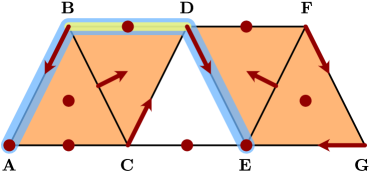
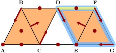
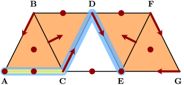
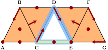
Figure 15. The stabilized combinatorial flow. For the gradient combinatorial vector field $\text{$\mathcal{V}$}_{3}$ introduced in the third row of Figure 6, the above four panels show the images $\Phi_{3}^{\infty}(x)$ for the one-dimensional critical cells $x$. From top left to bottom right they depict the chains $\Phi_{3}^{\infty}(\mathbf{B}\mathbf{D})$, $\Phi_{3}^{\infty}(\mathbf{D}\mathbf{F})$, $\Phi_{3}^{\infty}(\mathbf{A}\mathbf{C})$, and $\Phi_{3}^{\infty}(\mathbf{C}\mathbf{E})$, respectively, in blue.

We close this section with the following three examples. In the first of these, it will be demonstrated how the connection matrices in Table 2 can be determined using Theorem 8.21.

Example 8.23 (Three Forman gradient vector fields).

Consider the gradient combinatorial Forman vector field $\text{$\mathcal{V}$}_{3}$ which was introduced in the third row of Figure 6. By following the arguments in Example 8.13, one can easily show that $\Phi_{3}^{\infty}(x)=x$ for all zero-dimensional critical cells $x$. Moreover, we have both $\Phi_{3}^{\infty}(\mathbf{A}\mathbf{B}\mathbf{C})=\mathbf{A}\mathbf{B}\mathbf{C}+\mathbf{B}\mathbf{C}\mathbf{D}$ and $\Phi_{3}^{\infty}(\mathbf{E}\mathbf{F}\text{$\mathbf{G}$})=\mathbf{E}\mathbf{F}\text{$\mathbf{G}$}+\mathbf{D}\mathbf{E}\mathbf{F}$. For the four one-dimensional critical cells $y$, their images $\Phi_{3}^{\infty}(y)$ are illustrated in Figure 15.

The images under the stabilized flow $\Phi_{3}^{\infty}$ form the basis with respect to which one can determine the connection matrix. As before, we abbreviate these by $\bar{c}=\Phi_{3}^{\infty}(c)$ for all critical cells $c\in X^{c}$. Using this notation, for example in order to determine the last column of the third connection matrix in Table 2, we have to express the boundary $\partial\overline{\mathbf{E}\mathbf{F}\text{$\mathbf{G}$}}$ in terms of the chains $\bar{y}$ for the one-dimensional critical cells $y$, which leads to the identity

$$\partial\overline{\mathbf{E}\mathbf{F}\text{$\mathbf{G}$}}=\mathbf{D}\mathbf{F}+\mathbf{F}\text{$\mathbf{G}$}+\mathbf{E}\text{$\mathbf{G}$}+\mathbf{D}\mathbf{E}=\overline{\mathbf{D}\mathbf{F}},$$

and this accounts for the single entry of $1$ in the corresponding column given in Table 2. Similarly, since we have

$$\partial\overline{\mathbf{A}\mathbf{B}\mathbf{C}}=\mathbf{A}\mathbf{B}+\mathbf{B}\mathbf{D}+\mathbf{C}\mathbf{D}+\mathbf{A}\mathbf{C}=\overline{\mathbf{A}\mathbf{C}}+\overline{\mathbf{B}\mathbf{D}},$$

since the edge $\mathbf{D}\mathbf{E}$ which is contained in both of the last two chains cancels upon addition with respect to $\mbox{$\mathbb{Z}$}_{2}$-coefficients. This leads to the two nonzero entries in the second-to-last column of the last connection matrix in Table 2. The remaining columns can be determined analogously. $\Diamond$

Next, we briefly sketch how the above example can be used to determine connection matrices in the case of a combinatorial vector field which is not gradient. For this, we return to the setting of Figure 2.

Example 8.24 (A Forman vector field with periodic orbit).

Consider again the combinatorial vector field $\text{$\mathcal{V}$}_{0}$ from Figure 2, which has already been discussed in Examples 2.6 and 2.18. This vector field has a periodic orbit which traverses the vertices $\mathbf{C}$, $\mathbf{D}$, and $\mathbf{E}$ — and by breaking this periodic orbit into the union of two critical cells of dimensions $0$ and $1$, as well as the associated connecting orbits, we arrived at the three gradient systems $\text{$\mathcal{V}$}_{k}$ for $k=1,2,3$ shown in Figure 6.

We now claim that each of the connection matrices from Table 2 are in fact connection matrices for $\text{$\mathcal{V}$}_{0}$. Note that this vector field has a Morse decomposition $\text{$\mathcal{M}$}_{0}$ in which one Morse set, say $M_{p}$, consists of the periodic orbit. Since the associated Conley index has the Conley polynomial $t+1$, we now further subdivide this Morse set into a critical cell $M_{\tilde{p}_{1}}$ of index $1$, one critical cell $M_{\tilde{p}_{0}}$ of index $0$, as well as two Forman vectors, as shown in Figure 6. This results in one of the combinatorial vector fields $\text{$\mathcal{V}$}_{k}$, which in turn leads to a refinement of the associated acyclic partitions used in Definition 7.13. But then a direct application of Propositions 6.13 and 6.15 shows that the Conley complex associated with $\text{$\mathcal{V}$}_{k}$ is also a Conley complex for $\text{$\mathcal{V}$}_{0}$. (Note in particular that the above introduction of the critical cells $M_{\tilde{p}_{1}}$ and $M_{\tilde{p}_{0}}$ implies that the Conley complex has a trivial boundary operator on the coarsened Morse set which includes the periodic orbit in $\text{$\mathcal{M}$}_{0}$.) In other words, the connection matrices shown in Table 2 are also connection matrices for $\text{$\mathcal{V}$}_{0}$.

In fact, even more is true. Not only are all three connection matrices from Table 2 connection matrices for $\text{$\mathcal{V}$}_{0}$, they are also pairwise nonequivalent in the sense of Definition 5.21, that is, the vector field $\text{$\mathcal{V}$}_{0}$ does not have a unique connection matrix. In the remainder of this example, we briefly sketch the necessary proof of nonequivalence.

For this, we only consider the vector fields $\text{$\mathcal{V}$}_{1}$ and $\text{$\mathcal{V}$}_{2}$. In view of Propositions 8.18 and 8.19 the transfer morphism $T:\text{$\mathcal{C}$}^{\prime}\to\text{$\mathcal{C}$}^{\prime\prime}$ from the Conley complex $(\text{$\mathcal{M}$}_{0},\text{$\mathcal{C}$}^{\prime},d^{\prime})$ associated with $\text{$\mathcal{V}$}_{1}$ to the Conley complex $(\text{$\mathcal{M}$}_{0},\text{$\mathcal{C}$}^{\prime\prime},d^{\prime\prime})$ associated with $\text{$\mathcal{V}$}_{2}$ is defined via the formula

$$T(\bar{c})=\Phi_{2}^{\infty}\left(\Phi_{1}^{\infty}(c)\right)\quad\mbox{ for }\quad\bar{c}=\Phi_{1}^{\infty}(c)\;.$$

Furthermore, the matrix representations of the boundary operators $d^{\prime}$ and $d^{\prime\prime}$ can be found in the first two entries of Table 2.

As before we suppose that there exists a graded morphism $f$ and a degree $+1$ homomorphism $\Gamma:C^{\prime}\to C^{\prime\prime}$ with

$$T-f=d^{\prime\prime}\Gamma+\Gamma d^{\prime}\;.$$

We now evaluate both sides of this equation at the chain $\overline{\mathbf{D}\mathbf{F}}$. The first matrix in Table 2 shows that $d^{\prime}(\overline{\mathbf{D}\mathbf{F}})=0$. Furthermore, quick glances at Figures 13 and 14 imply that $T(\overline{\mathbf{D}\mathbf{F}})=\overline{\mathbf{D}\mathbf{F}}+\overline{\mathbf{D}\mathbf{E}}$. Finally, since $f$ is a graded morphism we have to have $f(\overline{\mathbf{D}\mathbf{F}})=\alpha\overline{\mathbf{D}\mathbf{F}}$ for some $\alpha\in\mbox{$\mathbb{Z}$}_{2}$. Substituting these into the above identity relating $T$ and $f$ one then obtains

$$\overline{\mathbf{D}\mathbf{F}}+\overline{\mathbf{D}\mathbf{E}}-\alpha\overline{\mathbf{D}\mathbf{F}}=d^{\prime\prime}(\Gamma(\overline{\mathbf{D}\mathbf{F}}))\;.$$

This equation, however, is impossible for $\alpha=1$ due to the matrix form of $d^{\prime\prime}$ given in Table 2, since $(0,0,1,0,0,0)^{t}$ (which corresponds to the chain $\overline{\mathbf{D}\mathbf{E}}$) is not contained in the column space of the matrix of $d^{\prime\prime}$. On the other hand, if $\alpha=0$, then the form of $d^{\prime\prime}$ immediately implies $\Gamma(\overline{\mathbf{D}\mathbf{F}})=\overline{\mathbf{E}\mathbf{F}\text{$\mathbf{G}$}}$, and since $\Gamma$ is filtered this furnishes $\overline{\mathbf{E}\mathbf{F}\text{$\mathbf{G}$}}\leq\overline{\mathbf{D}\mathbf{F}}$, a contradiction. In other words, the connection matrices arising from the vector fields $\text{$\mathcal{V}$}_{1}$ and $\text{$\mathcal{V}$}_{2}$ are not equivalent in the sense of Definition 5.21.

The nonequivalence proofs for $\text{$\mathcal{V}$}_{1}\not\equiv\text{$\mathcal{V}$}_{3}$, as well as $\text{$\mathcal{V}$}_{2}\not\equiv\text{$\mathcal{V}$}_{3}$, are similar and thus left to the reader. We would like to point out, however, that the first of these two cases requires a slightly more involved argument. $\Diamond$

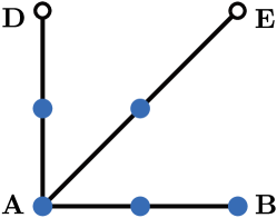
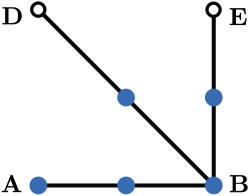
Figure 16. Conley complexes $(\bar{X},\partial^{\bar{\kappa}})$ for the Morse decompositions $\text{$\mathcal{M}$}_{1}$ (left) and $\text{$\mathcal{M}$}_{2}$ (right) of the combinatorial gradient vector fields $\text{$\mathcal{V}$}_{1}$ and $\text{$\mathcal{V}$}_{2}$ in Figure 11, visualized as $\kappa$-subcomplexes of simplicial complexes.

As our last example, we return to the discussions begun in Examples 5.12 and 5.23, which center on the combinatorial flows in Figure 11.

Example 8.25.

Consider the partition $\text{$\mathcal{E}$}_{1}:=\text{$\mathcal{E}$}_{\text{$\mathcal{M}$}_{1}}$ associated with the Morse decomposition $\text{$\mathcal{M}$}_{1}$ of the vector field $\text{$\mathcal{V}$}_{1}$ in the middle of Figure 11. In this simple case it coincides with the vector field $\text{$\mathcal{V}$}_{1}$. Hence, the Hasse diagram of the partial order $\leq_{\text{$\mathcal{E}$}_{1}}$ coincides with diagram (87). It follows that $\text{$\mathcal{V}$}_{1}$ is a gradient vector field and by Theorem 8.21 the Morse decomposition $\text{$\mathcal{M}$}_{1}$ has exactly one connection matrix. One can verify that the morphisms $(\varepsilon,h^{\prime})$ and $(\varepsilon^{-1},g^{\prime})$ constructed as in Example 5.12 are also filtered with respect to the filtration $(\text{$\mathcal{E}$}_{1},C(X),\partial^{\kappa})$. Therefore, arguing as in Example 5.12 we conclude that the Conley complex of $\text{$\mathcal{M}$}_{1}$ is the filtered chain complex in Example 4.15 with the associated connection matrix (41). In fact, the homomorphism $h^{\prime}$ coincides with the homomorphism $\Phi_{\text{$\mathcal{V}$}_{1}}$, and we have $\Phi_{\text{$\mathcal{V}$}_{1}}=\Phi_{\text{$\mathcal{V}$}_{1}}^{\infty}$ in this case. An analogous argument shows that the Conley complex of $\text{$\mathcal{M}$}_{2}$ is the filtered chain complex in Example 5.23 with the associated connection matrix (68). Both Conley complexes are visualized in Figure 16 as $\kappa$-subcomplexes of suitable simplicial complexes. $\Diamond$

9. Future work and open problems

The main goal of the present paper was to carry over the classical theory of connection matrices to the case of multivector fields on Lefschetz complexes. Yet, in the course of this we achieved even more. By allowing for the change of poset in the underlying Morse decomposition, we now have a mechanism at hand to compare and ultimately classify connection matrices. In contrast to existing results, this makes it possible to give a precise meaning to the phenomenon of multiple connection matrices. As a welcome side effect, we could also shorten the connection matrix pipeline described in the introduction. Combined with the recent development of concrete algorithms for the computation of connection matrices, this should considerably broaden their applicability in concrete examples.

Nevertheless, the results presented in this paper are just a first step. There are a number of important open questions that have to be addressed in the future, and which will be briefly outlined in the following.

• While our definitions give a precise definition that two connection matrices are the same, verifying this equivalence is not immediately straightforward. For this, it is necessary to recognize a morphism as essentially graded. Are there easy ways to do this?

• Related to the previous point, are there easy ways to see that two connection matrices are really different, i.e., that one is in the situation of a multivector field with multiple connection matrices? Are there easily computable invariants that can be used to detect this?

• What is the deeper meaning of the occurrence of multiple connection matrices? In the classical case, this is always seen as an indication of dynamical objects such as saddle-saddle connections. Is the same true in the combinatorial multivector case?

• In the classical case, transition matrices encode global bifurcations that can be detected using a change in connection matrices. Can this notion be extended to the combinatorial multivector case? In fact, we suppose that this is strongly related to our notion of transfer morphisms. In what way precisely? In order to address this question, one also will have to establish a precise notion of continuation of connection matrices.

• Can every connection matrix be computed using the algorithms mentioned earlier? We have indicated through examples that in certain cases it is possible to break up recurrent Morse sets in such a way that the resulting multivector field is actually gradient. Are the connection matrices obtained in this way all possible connection matrices? If not, is it possible to obtain the remaining ones algorithmically?

• The earlier mentioned persistence based connection matrix algorithm indicates the possibility of the interpretation of connection matrix theory in the language of persistence. Such a possibility might lead to applications of connection matrices which go beyond dynamics.

Progress on any of these topics would only serve to extend the range of potential applications of this theory.

References

- [1] P. Alexandrov. Diskrete Räume. Mathematiceskii Sbornik (N.S.), 2:501–518, 1937.
- [2] J. A. Barmak. Algebraic Topology of Finite Topological Spaces and Applications, volume 2032 of Lecture Notes in Mathematics. Springer-Verlag, Berlin – Heidelberg, 2011.
- [3] J. A. Barmak, M. Mrozek, and T. Wanner. A Lefschetz fixed point theorem for multivalued maps of finite spaces. Mathematische Zeitschrift, 294(3–4):1477–1497, 2020.
- [4] B. Batko, T. Kaczynski, M. Mrozek, and T. Wanner. Linking combinatorial and classical dynamics: Conley index and Morse decompositions. Foundations of Computational Mathematics, 20(5):967–1012, 2020.
- [5] G. Birkhoff. Rings of sets. Duke Math. J., 3(3):443–454, 1937.
- [6] C. Conley. Isolated invariant sets and the Morse index, volume 38 of CBMS Regional Conference Series in Mathematics. American Mathematical Society, Providence, R.I., 1978.
- [7] T. K. Dey, M. Juda, T. Kapela, J. Kubica, M. Lipinski, and M. Mrozek. Persistent Homology of Morse Decompositions in Combinatorial Dynamics. SIAM Journal on Applied Dynamical Systems, 18:510–530, 2019.
- [8] T. K. Dey, M. Lipiński, M. Mrozek, and R. Slechta. Connection matrices through the lens of persistence. arXiv e-prints, page arXiv:2303.02549, 2023.
- [9] P. Dłotko, T. Kaczynski, M. Mrozek, and T. Wanner. Coreduction homology algorithm for regular CW-complexes. Discrete & Computational Geometry, 46(2):361–388, 2011.
- [10] R. Engelking. General Topology. Heldermann Verlag, Berlin, 1989.
- [11] R. Forman. Combinatorial vector fields and dynamical systems. Math. Z., 228(4):629–681, 1998.
- [12] R. Forman. Morse theory for cell complexes. Adv. Math., 134(1):90–145, 1998.
- [13] R. D. Franzosa. The connection matrix theory for Morse decompositions. Trans. Amer. Math. Soc., 311(2):561–592, 1989.
- [14] S. Harker, K. Mischaikow, and K. Spendlove. A computational framework for connection matrix theory. J. Appl. Comput. Topol., 5(3):459–529, 2021.
- [15] M. Jöllenbeck and V. Welker. Minimal resolutions via algebraic discrete Morse theory. Mem. Amer. Math. Soc., 197(923):vi+74, 2009.
- [16] T. Kaczynski, K. Mischaikow, and M. Mrozek. Computational homology, volume 157 of Applied Mathematical Sciences. Springer-Verlag, New York, 2004.
- [17] T. Kaczynski, M. Mrozek, and M. Ślusarek. Homology computation by reduction of chain complexes. Comp. Math. Appl., 35:59–70, 1998.
- [18] T. Kaczynski, M. Mrozek, and T. Wanner. Towards a formal tie between combinatorial and classical vector field dynamics. J. Comput. Dyn., 3(1):17–50, 2016.
- [19] W. Kalies, K. Mischaikow, and R. Vandervorst. Lattice structures for attractors III. J. Dynam. Diff. Equ., 34:1729–1768, 2022.
- [20] K. P. Knudson. Morse theory: smooth and discrete. World Scientific, 2015.
- [21] D. Kozlov. Combinatorial Algebraic Topology, volume 21. Springer, Berlin, 2008.
- [22] S. Lang. Algebra, volume 211 of Graduate Texts in Mathematics. Springer-Verlag, New York, third edition, 2002.
- [23] S. Lefschetz. Algebraic Topology. American Mathematical Society Colloquium Publications, v. 27. American Mathematical Society, New York, 1942.
- [24] M. Lipiński, J. Kubica, M. Mrozek, and T. Wanner. Conley-Morse-Forman theory for generalized combinatorial multivector fields on finite topological spaces. Journal of Applied and Computational Topology, 2023. To appear.
- [25] W. S. Massey. A Basic Course in Algebraic Topology. Graduate Texts in Mathematics, v. 127. Springer-Verlag, New York, 1991.
- [26] M. C. McCord. Singular homology groups and homotopy groups of finite topological spaces. Duke Math. J., 33:465–474, 1966.
- [27] M. Mrozek. Conley-Morse-Forman theory for combinatorial multivector fields on Lefschetz complexes. Found. Comput. Math., 17(6):1585–1633, 2017.
- [28] M. Mrozek and B. Batko. Coreduction homology algorithm. Discrete Comput. Geom., 41(1):96–118, 2009.
- [29] M. Mrozek, R. Srzednicki, J. Thorpe, and T. Wanner. Combinatorial vs. classical dynamics: Recurrence. Communications in Nonlinear Science and Numerical Simulation, 108:Paper No. 106226, 30 pp, 2022.
- [30] M. Mrozek and T. Wanner. Creating semiflows on simplicial complexes from combinatorial vector fields. Journal of Differential Equations, 304:375–434, 2021.
- [31] J. R. Munkres. Elements of Algebraic Topology. Addison-Wesley, 1984.
- [32] J. R. Munkres. Topology. Prentice Hall, Inc., Upper Saddle River, NJ, 2000.
- [33] J. F. Reineck. The connection matrix in Morse-Smale flows. Trans. Amer. Math. Soc., 322(2):523–545, 1990.
- [34] J. F. Reineck. The connection matrix in Morse-Smale flows. II. Trans. Amer. Math. Soc., 347(6):2097–2110, 1995.
- [35] J. W. Robbin and D. A. Salamon. Lyapunov maps, simplicial complexes and the Stone functor. Ergodic Theory Dynam. Systems, 12(1):153–183, 1992.
- [36] E. Sköldberg. Morse theory from an algebraic viewpoint. Trans. Amer. Math. Soc., 358:115–129, 2005.