Student-Teacher Feature Pyramid Matching for Anomaly Detection

Abstract

Anomaly detection is a challenging task and usually formulated as an one-class learning problem for the unexpectedness of anomalies. This paper proposes a simple yet powerful approach to this issue, which is implemented in the student-teacher framework for its advantages but substantially extends it in terms of both accuracy and efficiency. Given a strong model pre-trained on image classification as the teacher, we distill the knowledge into a single student network with the identical architecture to learn the distribution of anomaly-free images and this one-step transfer preserves the crucial clues as much as possible. Moreover, we integrate the multi-scale feature matching strategy into the framework, and this hierarchical feature matching enables the student network to receive a mixture of multi-level knowledge from the feature pyramid under better supervision, thus allowing to detect anomalies of various sizes. The difference between feature pyramids generated by the two networks serves as a scoring function indicating the probability of anomaly occurring. Due to such operations, our approach achieves accurate and fast pixel-level anomaly detection. Very competitive results are delivered on the MVTec anomaly detection dataset, superior to the state of the art ones.

1 Introduction

Anomaly detection is generally referred to as identifying samples that are atypical with respect to regular patterns in the data set and has shown great potential in various real-world applications such as video surveillance [Abati et al.(2019)Abati, Porrello, Calderara, and Cucchiara, Roitberg et al.(2018)Roitberg, Al-Halah, and Stiefelhagen], product quality control [Bergmann et al.(2019)Bergmann, Fauser, Sattlegger, and Steger, Bergmann et al.(2020)Bergmann, Fauser, Sattlegger, and Steger, Napoletano et al.(2018)Napoletano, Piccoli, and Schettini] and medical diagnosis [Schlegl et al.(2019)Schlegl, Seeböck, Waldstein, Langs, and Schmidt-Erfurth, Schlegl et al.(2017)Schlegl, Seeböck, Waldstein, Schmidt-Erfurth, and Langs, Vasilev et al.(2018)Vasilev, Golkov, Lipp, Sgarlata, Tomassini, Jones, and Cremers]. Its key challenge lies in the unexpectedness of anomalies which is very difficult to deal with in a supervised way, as labeling all types of anomalous instances seems unrealistic.

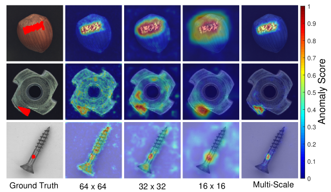
Figure 1: Visual results of our method on three defective images from the MVTec AD dataset. ResNet-18 is used as backbone and the three bottom blocks (i.e., conv2_x, conv3_x, conv4_x) are selected as feature extractors. Columns from left to right correspond to input images with defects (ground truth regions in red), anomaly maps of the three blocks, and the resulting anomaly maps respectively.

Previous studies address this challenge in the form of one-class learning paradigm [Moya et al.(1993)Moya, Koch, and Hostetler]. They approximate the decision boundary for a binary classification problem by searching a feature space where the distribution of normal data is accurately modeled. Deep learning, in particular convolutional neural networks (CNNs) [LeCun et al.(1998)LeCun, Bottou, Bengio, and Haffner] and residual networks (ResNets) [He et al.(2016)He, Zhang, Ren, and Sun], provides a powerful alternative to automatically build comprehensive representations at multiple levels. Such deep features prove very effective in capturing the intrinsic characteristics of the normal data manifold [An and Cho(2015), Chalapathy et al.(2018)Chalapathy, Menon, and Chawla, Masana et al.(2018)Masana, Ruiz, Serrat, Joost, and Lopez, Ruff et al.(2018)Ruff, Vandermeulen, Görnitz, Deecke, Siddiqui, Binder, Müller, and Kloft, Zhou and Paffenroth(2017)]. Despite the promising results in their respective fields, all these methods simply predict anomalies at the image-level without spatial localization.

The pixel-level methods advance anomaly detection by means of pixel-wise comparison of image patches and their reconstructions [Baur et al.(2018)Baur, Wiestler, Albarqouni, and Navab, Schlegl et al.(2019)Schlegl, Seeböck, Waldstein, Langs, and Schmidt-Erfurth, Schlegl et al.(2017)Schlegl, Seeböck, Waldstein, Schmidt-Erfurth, and Langs] or per-pixel estimation of probability density on entire images [Abati et al.(2019)Abati, Porrello, Calderara, and Cucchiara, Seeböck et al.(2016)Seeböck, Waldstein, Klimscha, Donner, Schlegl, Schmidt-Erfurth, and Langs], among which Auto-encoders, Generative Adversarial Networks (GANs), and their variants are dominating models. However, their performance is prone to serious degradation when images are poorly reconstructed  [Paul Bergmann and Steger(2019)] or likelihoods are inaccurately calibrated [Nalisnick et al.(2019)Nalisnick, Matsukawa, Teh, Gorur, and Lakshminarayanan].

Some recent attempts transfer the knowledge from other well-studied computer vision tasks. They directly apply the networks pre-trained on image classification and show that they are sufficiently generic to image-level detection [Andrews et al.(2016)Andrews, Tanay, Morton, and Griffin, Burlina et al.(2019)Burlina, Joshi, and Wang, Erfani et al.(2016)Erfani, Rajasegarar, Karunasekera, and Leckie]. Cohen and Hoshen [Cohen and Hoshen(2020)] investigate this idea in pixel-level detection and delivers performance gain; unfortunately, it has the time bottleneck due to per-pixel comparison. Bergmann et al. [Bergmann et al.(2020)Bergmann, Fauser, Sattlegger, and Steger] utilize the pre-trained model in a more efficient way by implicitly learning the distribution of normal features with a student-teacher framework and reach decent results. The difference between the outputs of the students and teacher along with the uncertainty among students’ predictions serves as the anomaly scoring function. Nevertheless, two major drawbacks still remain: i.e., the incompleteness of transferred knowledge and complexity of handling scaling. For the former, since knowledge is distilled from a ResNet-18 [He et al.(2016)He, Zhang, Ren, and Sun] into a lightweight teacher network, the big gap between their model capacities [Wang and Yoon(2020)] tends to incur loss of important information. For the latter, multiple student-teacher ensemble pairs are required to be separately trained, each for a specific respective field, to achieve scale invariance, which leads to the inconvenience in computation. Both the facts leave much room for improvement.

In this paper, we propose a simple yet powerful approach to anomaly detection, which follows the student-teacher framework for the advantages but substantially extends it in terms of both accuracy and efficiency. Specifically, given a powerful network pre-trained on image classification as the teacher, we distill the knowledge into a single student network with the identical architecture. In this case, the student network learns the distribution of anomaly-free images by matching their features with the counterparts of the pre-trained network, and this one-step transfer preserves the crucial information as much as possible. Furthermore, to enhance the scale robustness, we embed multi-scale feature matching into the network, and this hierarchical feature matching strategy enables the student network to receive a mixture of multi-level knowledge from the feature pyramid under a stronger supervision and thus allows to detect anomalies of various sizes (see Figure 1 for visualization). The feature pyramids from the teacher and student networks are compared for prediction, where a larger difference indicates a higher probability of anomaly occurrence.

Compared to the previous work, especially the preliminary student-teacher model, the benefits of our approach are two-fold. First, useful knowledge is well transferred from the pre-trained network to the student network within one-step distillation, as they share the same structure. Second, thanks to the hierarchical structure of the network, multi-scale anomaly detection is conveniently reached by the proposed feature pyramid matching scheme. Due to such strengths, our approach conducts accurate and fast pixel-level anomaly detection. It reports very competitive results on the MVTec anomaly detection dataset, and more results on ShanghaiTech Campus (STC) [Luo et al.(2017)Luo, Liu, and Gao] and CIFAR-10 [Krizhevsky and Hinton(2009)] are presented in the supplementary material.

2 Related Work

2.1 Image-level Anomaly Detection

Image-level techniques manifest anomalies in images of unseen categories. They can be coarsely divided into: reconstruction-based, distribution-based and classification-based.

The first group of approaches reconstruct the training images to capture the normal data manifold. An anomalous image is very likely to possess a high reconstruction error during inference, as it is drawn from a different distribution. The main weakness of these approaches comes from the excellent generalization ability of the deep models, including variational autoencoder [An and Cho(2015)], robust autoencoder [Zhou and Paffenroth(2017)], conditional GAN [Akcay et al.(2018)Akcay, Atapour-Abarghouei, and Breckon], and bi-directional GAN [Zenati et al.(2018)Zenati, Romain, Foo, Lecouat, and Chandrasekhar], which probably allows anomalous images to be faithfully reconstructed.

Distribution-based approaches model the probabilistic distribution of the normal images. The images that have low probability density values are designated as anomalous. Recent algorithms such as anomaly detection GAN (ADGAN) [Deecke et al.(2018)Deecke, Vandermeulen, Mandt, and Kloft] and deep autoencoding Gaussian mixture model (DAGMM) [Zong et al.(2018)Zong, Song, Min, Cheng, Lumezanu, Cho, and Chen] learn a deep projection that maps high-dimensional images into a low-dimensional latent space. Nevertheless, these methods have high sample complexity and demand large training data.

Classification-based approaches have dominated anomaly detection in the last decade. One useful paradigm is to feed the deep features extracted by deep generative models [Burlina et al.(2019)Burlina, Joshi, and Wang] or transferred from pre-trained networks [Andrews et al.(2016)Andrews, Tanay, Morton, and Griffin, Erfani et al.(2016)Erfani, Rajasegarar, Karunasekera, and Leckie] into a separate shallow classification model like one-class support vector machine (OC-SVM) [Schölkopf et al.(2001)Schölkopf, Platt, Shawe-Taylor, Smola, and Williamson]. Another line of research depends on self-supervised learning. Geom [Golan and El-Yaniv(2018)] creates a dataset by applying dozens of geometric transformations to the normal images and trains a multi-class neural network over the self-labeled dataset to discriminate such transformations. At test time, anomalies are expected to be assigned with less confidence in discriminating the transformations.

2.2 Pixel-level Anomaly Detection

Pixel-level techniques are particularly designed for anomaly localization. They aim to precisely segment anomalous regions in images, which is more complicated than binary classification.

The expressive power of deep neural networks inspires a series of studies that explore how to transfer the benefits of the networks pre-trained on image classification tasks to anomaly detection. Napoletano et al. [Napoletano et al.(2018)Napoletano, Piccoli, and Schettini] exploit a pre-trained ResNet-18 to embed cropped training image patches into a feature space, reduce the dimension of feature vectors by PCA, and model their distribution using K-means clustering. This method requires a large number of overlapping patches to obtain a spatial anomaly map at inference time, which results in coarse-grained maps and may become a performance bottleneck.

To avoid cropping image patches and accelerate feature extraction, Sabokrou et al. [Sabokrou et al.(2018)Sabokrou, Fayyaz, Fathy, Moayed, and Klette] build descriptors from early feature maps of a pre-trained fully convolutional network (FCN) and adopt a unimodal Gaussian distribution to fit feature vectors of the anomaly-free images. However, the unimodel Gaussian distribution fails to characterize the training feature distribution as the problem complexity increases. More recently, a convolutional adversarial variational autoencoder with guided attention (CAVGA) [Venkataramanan et al.(2020)Venkataramanan, Peng, Singh, and Mahalanobis] incorporates Grad-CAM [Selvaraju et al.(2017)Selvaraju, Cogswell, Das, Vedantam, and Parikh] into a variational autoencoder with an attention expansion loss to encourage the deep model itself to focus on all normal regions in the image. Simliar to typical autoencoders (AE) [Bergmann et al.(2019)Bergmann, Fauser, Sattlegger, and Steger, Paul Bergmann and Steger(2019)] and variational autoencoders (VAE) [Liu et al.(2020)Liu, Li, Zheng, Karanam, Wu, Bhanu, Radke, and Camps], CAVGA also suffers from the strong generalization ability which allows good reconstruction for anomalous images.

3 Method

3.1 Framework

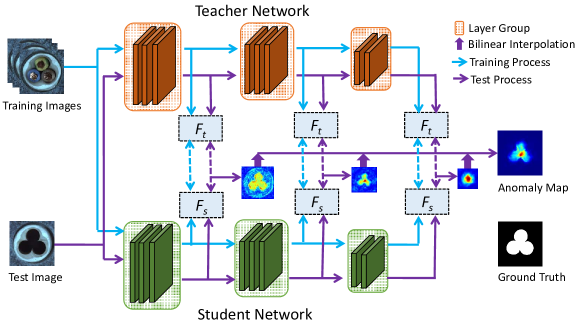
Figure 2: Schematic overview of our method. The feature pyramid of a student network is trained to match with the counterpart of a pre-trained teacher network. A test image (or pixel) has a high anomaly score if its features from the two models differ significantly. The feature pyramid matching enables our method to detect anomalies of various sizes with a single forward pass.

We make use of the student-teacher learning framework to implicitly model the feature distribution of the normal training images. The teacher is a powerful network pre-trained on the image classification task (e.g., a ResNet-18 pre-trained on ImageNet). To reduce information loss, the student shares the same architecture with the teacher. This is in essence one case of feature-based knowledge distillation [Wang and Yoon(2020)].

Here, we need to consider a key factor, i.e., position of distillation. Deep neural networks generate a pyramid of features for each input image. Bottom layers result in higher-resolution features encoding low-level information such as textures, edges and colors. By contrast, top layers yield low-resolution features that contain context information. The features created by bottom layers are often generic enough and they can be shared by various vision tasks [Oquab et al.(2014)Oquab, Bottou, Laptev, and Sivic, Zeiler and Fergus(2014)]. This motivates us to integrate low-level and high-level features in a complementary way. As different layers in deep neural networks correspond to distinct receptive fields, we select the features extracted by a few successive bottom layer groups (e.g., blocks in ResNet-18) of the teacher to guide the student’s learning. This hierarchical feature matching allows our method to detect anomalies of various sizes.

Figure 2 gives a sketch of our method with the images from the MVTec AD dataset [Bergmann et al.(2020)Bergmann, Fauser, Sattlegger, and Steger] as examples. The training and test processes are formally provided as follows.

3.2 Training Process

The training phase aims to obtain a good student which can perfectly imitate the outputs of a fixed teacher on normal images. Formally, given a training dataset of anomaly-free images $\mathcal{D}=\{\mathbf{I}_{1},\mathbf{I}_{2},\dots,\mathbf{I}_{n}\}$, our goal is to capture the normal data manifold by matching the features extracted by the $L$ bottom layer groups of the teacher with the counterparts of the student. For an input image $\mathbf{I}_{k}\in\mathbb{R}^{w\times h\times c}$, where $h$ is the height, $w$ is the width and $c$ is the number of the color channels, the $l$th bottom layer group of the teacher and student outputs a feature map $F^{l}_{t}(\mathbf{I}_{k})\in\mathbb{R}^{w_{l}\times h_{l}\times d_{l}}$ and $F^{l}_{s}(\mathbf{I}_{k})\in\mathbb{R}^{w_{l}\times h_{l}\times d_{l}}$, where $w_{l}$, $h_{l}$ and $d_{l}$ denote the width, height and channel number of the feature map, respectively. Since there is no prior knowledge regarding the appearances and locations of objects, we simply assume that all image regions are anomaly-free in the training set. Note that $F^{l}_{t}(\mathbf{I}_{k})_{ij}\in\mathbb{R}^{d_{l}}$ and $F^{l}_{s}(\mathbf{I}_{k})_{ij}\in\mathbb{R}^{d_{l}}$ are feature vectors at position $(i,j)$ in the feature maps from the teacher and student, respectively. We define the loss at position $(i,j)$ as $\ell_{2}$-distance between the $\ell_{2}$-normalized feature vectors, namely,

$$\ell^{l}(\mathbf{I}_{k})_{ij}=\frac{1}{2}\left\|\hat{F}^{l}_{t}(\mathbf{I}_{k})_{ij}-\hat{F}^{l}_{s}(\mathbf{I}_{k})_{ij}\right\|^{2}_{\ell_{2}},$$ (1)

$$\hat{F}^{l}_{t}(\mathbf{I}_{k})_{ij}=\frac{F^{l}_{t}(\mathbf{I}_{k})_{ij}}{\|F^{l}_{t}(\mathbf{I}_{k})_{ij}\|_{\ell_{2}}},\,\,\,\hat{F}^{l}_{s}(\mathbf{I}_{k})_{ij}=\frac{F^{l}_{s}(\mathbf{I}_{k})_{ij}}{\|F^{l}_{s}(\mathbf{I}_{k})_{ij}\|_{\ell_{2}}}.$$

It is worth noting that the $\ell_{2}$ distance used in (Eq. 1) is proportional to the cosine distance as $F^{l}_{t}(\mathbf{I}_{k})$ and $F^{l}_{s}(\mathbf{I}_{k})$ are $\ell_{2}$-normalized vectors. Thus the loss $\ell^{l}(\mathbf{I}_{k})_{ij}\in(0,1)$. The loss for the entire image $\mathbf{I}_{k}$ is given as an average of the loss at each position,

$$\ell^{l}(\mathbf{I}_{k})=\frac{1}{w_{l}h_{l}}\sum_{i=1}^{w_{l}}\sum_{j=1}^{h_{l}}\ell^{l}(\mathbf{I}_{k})_{ij},$$ (2)

and the total loss is the weighted average of the loss at different pyramid scales,

$$\ell(\mathbf{I}_{k})=\sum_{l=1}^{L}\alpha_{l}\ell^{l}(\mathbf{I}_{k}),\quad\text{s.t.}\,\,\,\alpha_{l}\geq 0,\,\,\$$ (3)

where $\alpha_{l}$ depicts the impact of the $l$th feature scale on anomaly detection. We simply set $\alpha_{l}=1,l=1,\dots,L$ in all our experiments. Given a minibatch $\mathcal{B}$ sampled from the training dataset $\mathcal{D}$, we update the student by minimizing the loss $\ell_{\mathcal{B}}=\frac{1}{|\mathcal{B}|}\sum_{k\in\mathcal{B}}\ell(\mathbf{I}_{k})$. Note that we only update the student while keeping the teacher fixed throughout the training phase.

3.3 Test Process

In the test phase, we aim to obtain an anomaly map $\Omega$ of size $w\times h$ regarding a test image $\mathbf{J}\in\mathbb{R}^{w\times h\times c}$. The score $\Omega_{ij}\in[0,1]$ indicates how much the pixel at position $(i,j)$ deviates from the training data manifold. We forward the test image $\mathbf{J}$ into the teacher and the student. Let $F^{l}_{t}(\mathbf{J})$ and $F^{l}_{s}(\mathbf{J})$ denote the feature maps generated by the $l$th bottom layer group of the teacher and the student, respectively. We can compute an anomaly map $\Omega^{l}(\mathbf{J})$ of size $w_{l}\times h_{l}$, whose element $\Omega^{l}_{ij}(\mathbf{J})$ is the loss (Eq. 1) at position $(i,j)$. The anomaly map $\Omega^{l}(\mathbf{J})$ is upsampled to size $w\times h$ by bilinear interpolation. The resulting anomaly map is defined as the element-wise product of $L$ equal-sized upsampled anomaly maps,

$$\Omega(\mathbf{J})=\prod_{l=1}^{L}\operatorname{Upsample}\Omega^{l}(\mathbf{J}).$$ (4)

A test image is designated as anomaly if any pixel in the image is anomalous. As a result, we simply choose the maximum value in the anomaly map, i.e., $\max(\Omega(\mathbf{J}))$ as the anomaly score for the test image $\mathbf{J}$.

4 Experiments

4.1 Dataset

We conduct experiments on the MVTec Anomaly Detection (MVTec AD) [Bergmann et al.(2019)Bergmann, Fauser, Sattlegger, and Steger] dataset, with both the image-level and pixel-level anomaly detection tasks considered. The dataset is specifically created to benchmark algorithms for anomaly localization. It collects more than 5,000 high-resolution images of industrial products covering 15 different categories. For each category, the training set only includes defect-free images and the test set comprises both defect-free images and defective images of different types. The performance is measured by two popular metrics: AUC-ROC and Per-Region-Overlap (PRO) [Bergmann et al.(2020)Bergmann, Fauser, Sattlegger, and Steger]. Supplementary material provides more results on ShanghaiTech Campus (STC) [Luo et al.(2017)Luo, Liu, and Gao] and CIFAR-10 [Krizhevsky and Hinton(2009)].

4.2 Implementation Details

For all the experiments, we choose the first three blocks (i.e., conv2_x, conv3_x, conv4_x) of ResNet-18 as the pyramid feature extractors for both the teacher and student networks. The parameters of the teacher network are copied from the ResNet-18 pre-trained on ImageNet, while those of the student network are initialized randomly. We train the network using stochastic gradient descent (SGD) with a learning rate of 0.4 for 100 epochs. The batch size is 32. All the images in the training and test sets are resized to 256$\times$256. For each category, we use 80% of training images to build the student, keeping the remaining 20% for validation. We select the checkpoint with the lowest validation error (Eq. 1) to perform anomaly detection.

4.3 Results

We begin with the task of finding anomalous images. As defective regions usually occupy a small proportion of the whole image, the test anomalies differ in a subtle way from the training images. This makes the MVTec AD dataset more challenging than those previously used in the literature (e.g., MNIST and CIFAR-10) where the images from the other categories are regarded as anomalous to the selected one. Table 2 compares our method to state-of-the-art approaches: Geom [Golan and El-Yaniv(2018)], GANomaly [Akcay et al.(2018)Akcay, Atapour-Abarghouei, and Breckon], $\l_{2}$-AE [Aytekin et al.(2018)Aytekin, Ni, Cricri, and Aksu], ITAE [Huang et al.(2020)Huang, Ye, Cao, Li, Zhang, and Lu], Cut-Paste [Li et al.(2021)Li, Sohn, Yoon, and Pfister] Patch-SVDD [Yi and Yoon(2020)], PaDiM [Defard et al.(2021)Defard, Setkov, Loesch, and Audigier] and SPADE [Cohen and Hoshen(2020)]. We clearly see that our approach outperforms all the other methods. In particular, the performance is improved up to 11.7% compared with SPADE [Cohen and Hoshen(2020)], which also leverages multi-scale features from a pre-trained model. It validates the superiority of the student-teacher learning framework.

Category SSIM-AE AnoGAN CNN-Dict^∗ STAD^∗ Cut-Paste Patch-SVDD PaDiM-R18^∗ SPADE^∗ Ours^∗ Textures Carpet 0.65 0.20 0.47 0.695 - - 0.960 0.947 0.958 0.87 0.54 0.72 - 0.983 0.926 0.989 0.975 0.988 Grid 0.85 0.23 0.18 0.819 - - 0.909 0.867 0.966 0.94 0.58 0.59 - 0.975 0.962 0.949 0.937 0.990 Leather 0.56 0.38 0.64 0.819 - - 0.979 0.972 0.980 0.78 0.64 0.87 - 0.995 0.974 0.991 0.976 0.993 Tile 0.18 0.18 0.80 0.912 - - 0.816 0.759 0.921 0.59 0.50 0.93 - 0.905 0.914 0.912 0.874 0.974 Wood 0.61 0.39 0.62 0.725 - - 0.903 0.874 0.936 0.73 0.62 0.91 - 0.955 0.908 0.936 0.885 0.972 Objects Bottle 0.83 0.62 0.74 0.918 - - 0.939 0.955 0.951 0.93 0.86 0.78 - 0.976 0.981 0.981 0.984 0.988 Cable 0.48 0.38 0.56 0.865 - - 0.862 0.909 0.877 0.82 0.78 0.79 - 0.900 0.968 0.958 0.972 0.955 Capsule 0.86 0.31 0.31 0.916 - - 0.919 0.937 0.922 0.94 0.84 0.84 - 0.974 0.958 0.983 0.990 0.983 Hazelnut 0.92 0.70 0.84 0.937 - - 0.914 0.954 0.943 0.97 0.87 0.72 - 0.973 0.975 0.977 0.991 0.985 Metal nut 0.60 0.32 0.36 0.895 - - 0.819 0.944 0.945 0.89 0.76 0.82 - 0.931 0.980 0.967 0.981 0.976 Pill 0.83 0.78 0.46 0.935 - - 0.906 0.946 0.965 0.91 0.87 0.68 - 0.957 0.951 0.947 0.965 0.978 Screw 0.89 0.47 0.28 0.928 - - 0.913 0.960 0.930 0.96 0.80 0.87 - 0.967 0.957 0.974 0.989 0.983 Toothbrush 0.78 0.75 0.15 0.863 - - 0.923 0.935 0.922 0.92 0.93 0.90 - 0.981 0.981 0.987 0.979 0.989 Transistor 0.73 0.55 0.63 0.701 - - 0.802 0.874 0.695 0.90 0.86 0.66 - 0.930 0.970 0.972 0.941 0.825 Zipper 0.67 0.47 0.70 0.933 - - 0.947 0.926 0.952 0.88 0.78 0.76 - 0.993 0.951 0.982 0.965 0.985 Mean 0.69 0.44 0.52 0.857 - - 0.901 0.917 0.921 0.87 0.74 0.78 - 0.960 0.957 0.967 0.965 0.970 • ^∗ denotes extra dataset pre-trained model used.

Table 1: Pixel-level anomaly detection. For each dataset category, PRO (top row) and AUC-ROC (bottom row) scores are given.

Geom GANomaly $\l_{2}$-AE ITAE Cut-Paste Patch-SVDD PaDiM-WR50^∗ SPADE^∗ Ours 0.672 0.762 0.754 0.839 0.952 0.921 0.953 0.855 0.955

• ^∗ denotes extra dataset pre-trained model used.

Table 2: Image-level anomaly detection. The performance is measured by average AUC-ROC across 15 categories.

We then consider the task of pixel-level anomaly detection and compare our method with the counterparts including Patch-SVDD [Yi and Yoon(2020)], PaMiD [Defard et al.(2021)Defard, Setkov, Loesch, and Audigier], etc. Table 1 reports the performance in terms of the AUC-ROC and PRO metrics. We notice two trends to achieve performance gains: (1) by pre-trained models, with a Wide-ResNet50$\times$2 network [Zagoruyko and Komodakis(2016)], SPADE reports very competitive scores; (2) by self-training techniques, Cut-Paste [Li et al.(2021)Li, Sohn, Yoon, and Pfister] and Patch-SVDD [Yi and Yoon(2020)] show this potential through designing proper pretext tasks for feature learning. As our approach assumes that anomaly detection is fulfilled via the heterogeneity of the student and teacher networks, i.e. different network parameters learned from individual data, we employ a pre-trained model built on generic images rather than self-supervised learning on the small scale anomaly detection dataset. As Table 1 displays, our approach delivers better performance than the others. It should be noted although STAD [Bergmann et al.(2020)Bergmann, Fauser, Sattlegger, and Steger] adopts the student-teacher learning framework, its performance is always inferior to that of our method. This gap can be attributed to the information loss in its two-step and single-scale knowledge transfer process. This validates our improvement in feature learning. When equipped with the same backbone as SPADE [Cohen and Hoshen(2020)], our method further boosts the results, i.e. 0.973 and 0.923 in AUC-ROC and PRO, respectively.

5 Ablation Studies and Discussions

We first perform feature visualization to investigate what the student learns from its teacher and also conduct ablation studies on the MVTec AD dataset to answer the following three questions. Is feature pyramid matching superior to single feature matching? Is the teacher pre-trained on other datasets still useful? Is our method applicable to small training dataset?

5.1 Feature Visualization

Figure 3 shows $t$-SNE visualization [Van der Maaten and Hinton(2008)] of learned features from the student and teacher. Obviously, the features from the student and teacher on normal regions distribute closer (even overlapped) than the ones on anomalous regions. It suggests that the student learns to match the teacher’s output on normal images. It also shows that the student well captures the distribution of normal patterns under the supervision of a good teacher.

(a) Bottle (broken$\_$large)

(b) Points at various positions

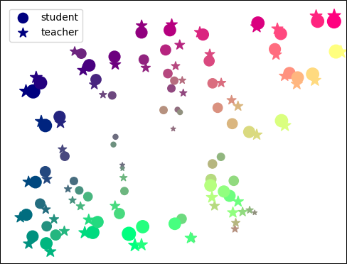
(c) t-SNE

Figure 3: $t$-SNE visualization [Van der Maaten and Hinton(2008)] of learned features from the student and teacher. (a) an example test image with defects contoured by a red line. (b) point map in which different positions are encoded by different sizes and colors. (c) $t$-SNE visualizations for features from the student (circle) and the teacher (star) with (a) as input. Zoomed in for better display.

5.2 Feature Matching

We first minutely investigate the effectiveness of feature extraction by each individual block of ResNet-18. Considering that the first block is a simple convolutional layer, we exclude it from comparison. We train the student by matching features extracted by its second, third, fourth and fifth blocks with the counterparts of the teacher respectively. As shown in Table 3, feature matching conducted at the end of the third and fourth blocks can achieve better performance. This is in good agreement with the previous discovery that the middle-level features play a more important role in knowledge transfer [Oquab et al.(2014)Oquab, Bottou, Laptev, and Sivic].

We then test three different combinations of the consecutive blocks of ResNet-18. Likewise, we match the features extracted from the corresponding compound blocks of the teacher and the student. Table 3 shows that the mixture of the second, third and fourth blocks outperforms other combinations as well as the single components. It implies that feature pyramid matching is a better way for feature learning. This finding is also validated in Figure 1. Anomaly maps generated by low-level features are more suitable for precise anomaly localization, but they are likely to include background noise. By contrast, anomaly maps generated by high-level features are able to segment big anomalous regions. The aggregation of anomaly maps at different scales contributes to accurate detection of anomalies of various sizes.

2 3 4 5 [2, 3] [2, 3, 4] [2, 3, 4, 5] AR_I 0.808 0.917 0.934 0.819 0.849 0.955 0.949 AR_P 0.915 0.953 0.957 0.860 0.950 0.970 0.969 PRO 0.815 0.897 0.835 0.504 0.886 0.921 0.886

Table 3: Ablation studies for feature matching. The performance is measured by the average image-level AUC-ROC (AR_I), average pixel-level AUC-ROC (AR_P) and average PRO across 15 categories.

5.3 Pre-trained Datasets

ImageNet MNIST CIFAR-10 CIFAR-100 SVHN AR_I 0.955 0.619 0.826 0.835 0.796 AR_P 0.970 0.759 0.931 0.937 0.902 PRO 0.921 0.528 0.863 0.842 0.742

Table 4: Ablation studies for pre-trained datasets. The performance is measured by the average image-level AUC-ROC (AR_I), average pixel-level AUC-ROC (AR_P) and average PRO across 15 categories.

To answer the second question, we pre-train the teacher on a couple of image classification benchmarks, including MNIST [LeCun and Cortes(2010)], CIFAR-10 [Krizhevsky and Hinton(2009)], CIFAR-100 [Krizhevsky and Hinton(2009)], and SVHN [Netzer et al.(2011)Netzer, Wang, Coates, Bissacco, Wu, and Ng]. These pre-trained teachers are individually exploited to guide the student training. The MNIST and SVHN datasets simply contain digital numbers from 0 to 9. We see from Table 4 that the teacher networks pre-trained on these two datasets yield worse results. It indicates that the features learned from these two pre-trained models generalize poorly on the MVTec AD dataset. By contrast, the features extracted from the teacher networks pre-trained on CIFAR-10 and CIFAR-100 exhibit better generalization, as they contain more natural images. Note that the performance of these two pre-trained teachers is still inferior to that of the teacher pre-trained on ImageNet. This is because that the ImageNet dataset consists of a huge number of high-resolution natural images, which is crucial to learning more discriminating features.

5.4 Number of Training Samples

We investigate the effect of the training set size in this experiment. Only 5% and 10% anomaly-free images are used to train our model. It can be seen in Table 5 that our model still reaches a satisfactory level even if only a few training images are available. By contrast, SPADE suffers a serious performance degradation. This is caused by the missing of the tailored feature learning. Our model profits from this strategy and can capture the feature distribution of anomaly-free images in the few-shot scenario. Furthermore, our method uses only 10% training samples to outperform the preliminary student-teacher framework [Bergmann et al.(2020)Bergmann, Fauser, Sattlegger, and Steger]. It validates the effectiveness of our feature pyramid matching technique.

5% 10% Metric Ours SPADE Ours SPADE AR_I 0.871 0.782 0.907 0.797 AR_P 0.961 0.932 0.967 0.955 PRO 0.892 0.842 0.913 0.890

Table 5: Performance in terms of the number of training samples. The performance is measured by the average image-level AUC-ROC (AR_I), average pixel-level AUC-ROC (AR_P) and average PRO across 15 categories.

6 Conclusion

We present a new feature pyramid matching technique and incorporate it into the student-teacher anomaly detection framework. Given a powerful network pre-trained on image classification as the teacher, we use its different levels of features to guide a student network with the same structure to learn the distribution of anomaly-free images. On account of the hierarchical feature matching, our method is capable of detecting anomalies of various sizes with only a single forward pass. Experimental results on the MVTec AD dataset show that our method achieves superior performance to the state-of-the-art.

References

- [Abati et al.(2019)Abati, Porrello, Calderara, and Cucchiara] Davide Abati, Angelo Porrello, Simone Calderara, and Rita Cucchiara. Latent space autoregression for novelty detection. In CVPR, 2019.
- [Akcay et al.(2018)Akcay, Atapour-Abarghouei, and Breckon] Samet Akcay, Amir Atapour-Abarghouei, and Toby P. Breckon. GANomaly: Semi-supervised anomaly detection via adversarial training. In ACCV, 2018.
- [An and Cho(2015)] Jinwon An and Sungzoon Cho. Variational autoencoder based anomaly detection using reconstruction probabiliy. Technical report, SNU Data Mining Center, 2015.
- [Andrews et al.(2016)Andrews, Tanay, Morton, and Griffin] Jerone T. A. Andrews, Thomas Tanay, Edward J. Morton, and Lewis D. Griffin. Transfer representation-learning for anomaly detection. In ICML Workshops, 2016.
- [Aytekin et al.(2018)Aytekin, Ni, Cricri, and Aksu] Caglar Aytekin, Xingyang Ni, Francesco Cricri, and Emre Aksu. Clustering and unsupervised anomaly detection with normalized deep auto-encoder representations. In IJCNN, 2018.
- [Baur et al.(2018)Baur, Wiestler, Albarqouni, and Navab] Christoph Baur, Benedikt Wiestler, Shadi Albarqouni, and Nassir Navab. Deep autoencoding models for unsupervised anomaly segmentation in brain mr images. In MICCAI Workshops, 2018.
- [Bergmann et al.(2019)Bergmann, Fauser, Sattlegger, and Steger] Paul Bergmann, Michael Fauser, David Sattlegger, and Carsten Steger. Mvtec AD - A comprehensive real-world dataset for unsupervised anomaly detection. In CVPR, 2019.
- [Bergmann et al.(2020)Bergmann, Fauser, Sattlegger, and Steger] Paul Bergmann, Michael Fauser, David Sattlegger, and Carsten Steger. Uninformed students: Student-teacher anomaly detection with discriminative latent embeddings. In CVPR, 2020.
- [Burlina et al.(2019)Burlina, Joshi, and Wang] Philippe Burlina, Neil Joshi, and I-Jeng Wang. Where’s wally now? deep generative and discriminative embeddings for novelty detection. In CVPR, 2019.
- [Chalapathy et al.(2018)Chalapathy, Menon, and Chawla] Raghavendra Chalapathy, Aditya Krishna Menon, and Sanjay Chawla. Anomaly detection using one-class neural networks. arXiv:1802.06360, 2018.
- [Cohen and Hoshen(2020)] Niv Cohen and Yedid Hoshen. Sub-image anomaly detection with deep pyramid correspondences. arXiv:2005.02357, 2020.
- [Deecke et al.(2018)Deecke, Vandermeulen, Mandt, and Kloft] Lucas Deecke, Robert Vandermeulen, Lukas RuffStephan Mandt, and Marius Kloft. Image anomaly detection with generative adversarial networks. In ECML-PKDD, pages 3–17, 2018.
- [Defard et al.(2021)Defard, Setkov, Loesch, and Audigier] Thomas Defard, Aleksandr Setkov, Angelique Loesch, and Romaric Audigier. Padim: A patch distribution modeling framework for anomaly detection and localization. In ICPR, 2021.
- [Erfani et al.(2016)Erfani, Rajasegarar, Karunasekera, and Leckie] Sarah M. Erfani, Sutharshan Rajasegarar, Shanika Karunasekera, and Christopher Leckie. High-dimensional and large-scale anomaly detection using a linear one-class svm with deep learning. Pattern Recognit., 58:121–134, 2016.
- [Golan and El-Yaniv(2018)] Izhak Golan and Ran El-Yaniv. Deep anomaly detection using geometric transformations. In NeurIPS, 2018.
- [He et al.(2016)He, Zhang, Ren, and Sun] Kaiming He, Xiangyu Zhang, Shaoqing Ren, and Jian Sun. Deep residual learning for image recognition. In CVPR, 2016.
- [Huang et al.(2020)Huang, Ye, Cao, Li, Zhang, and Lu] Chaoqin Huang, Fei Ye, Jinkun Cao, Maosen Li, Ya Zhang, and Cewu Lu. Attribute restoration framework for anomaly detection. arXiv:1911.10676, 2020.
- [Krizhevsky and Hinton(2009)] Alex Krizhevsky and Geoffrey Hinton. Learning multiple layers of features from tiny images. Technical report, University of Toronto, 2009.
- [LeCun and Cortes(2010)] Yann LeCun and Corinna Cortes. Mnist handwritten digit database. 2010.
- [LeCun et al.(1998)LeCun, Bottou, Bengio, and Haffner] Yann LeCun, Léon Bottou, Yoshua Bengio, and Patrick Haffner. Gradient-based learning applied to document recognition. Proc. IEEE, 86(11):2278–2324, 1998.
- [Li et al.(2021)Li, Sohn, Yoon, and Pfister] Chun-Liang Li, Kihyuk Sohn, Jinsung Yoon, and Tomas Pfister. Cutpaste: Self-supervised learning for anomaly detection and localization. In CVPR, 2021.
- [Liu et al.(2020)Liu, Li, Zheng, Karanam, Wu, Bhanu, Radke, and Camps] Wenqian Liu, Runze Li, Meng Zheng, Srikrishna Karanam, Ziyan Wu, Bir Bhanu, Richard J Radke, and Octavia Camps. Towards visually explaining variational autoencoders. In CVPR, 2020.
- [Luo et al.(2017)Luo, Liu, and Gao] Weixin Luo, Wen Liu, and Shenghua Gao. A revisit of sparse coding based anomaly detection in stacked rnn framework. In ICCV, 2017.
- [Masana et al.(2018)Masana, Ruiz, Serrat, Joost, and Lopez] Marc Masana, Idoia Ruiz, Joan Serrat, Van De Weijer Joost, and Antonio M Lopez. Metric learning for novelty and anomaly detection. In BMVC, 2018.
- [Moya et al.(1993)Moya, Koch, and Hostetler] M. M. Moya, M. W. Koch, and L. D. Hostetler. One-class classifier networks for target recognition applications. In WCCI, 1993.
- [Nalisnick et al.(2019)Nalisnick, Matsukawa, Teh, Gorur, and Lakshminarayanan] Eric Nalisnick, Akihiro Matsukawa, Yee Whye Teh, Dilan Gorur, and Balaji Lakshminarayanan. Do deep generative models know what they don’t know? In ICLR, 2019.
- [Napoletano et al.(2018)Napoletano, Piccoli, and Schettini] Paolo Napoletano, Flavio Piccoli, and Raimondo Schettini. Anomaly detection in nanofibrous materials by CNN-based self-similarity. Sensors, 18(2):209, 2018.
- [Netzer et al.(2011)Netzer, Wang, Coates, Bissacco, Wu, and Ng] Yuval Netzer, Tao Wang, Adam Coates, Alessandro Bissacco, Bo Wu, and Andrew Y. Ng. Reading digits in natural images with unsupervised feature learning. In NeurIPS Workshops, 2011.
- [Oquab et al.(2014)Oquab, Bottou, Laptev, and Sivic] Maxime Oquab, Léon Bottou, Ivan Laptev, and Josef Sivic. Learning and transferring mid-level image representations using convolutional neural networks. In CVPR, 2014.
- [Paul Bergmann and Steger(2019)] Michael Fauser David Sattlegger Paul Bergmann, Sindy Löwe and Carsten Steger. Improving unsupervised defect segmentation by applying structural similarity to autoencoders. In VISIGRAPP, 2019.
- [Roitberg et al.(2018)Roitberg, Al-Halah, and Stiefelhagen] Alina Roitberg, Ziad Al-Halah, and Rainer Stiefelhagen. Informed democracy: Voting-based novelty detection for action recognition. In BMVC, 2018.
- [Ruff et al.(2018)Ruff, Vandermeulen, Görnitz, Deecke, Siddiqui, Binder, Müller, and Kloft] Lukas Ruff, Robert A. Vandermeulen, Nico Görnitz, Lucas Deecke, Shoaib A. Siddiqui, Alexander Binder, Emmanuel Müller, and Marius Kloft. Deep one-class classification. In ICML, 2018.
- [Sabokrou et al.(2018)Sabokrou, Fayyaz, Fathy, Moayed, and Klette] Mohammad Sabokrou, Mohsen Fayyaz, Mahmood Fathy, Zahra Moayed, and Reinhard Klette. Deep-anomaly: Fully convolutional neural network for fast anomaly detection in crowded scenes. CVIU, 172, 2018.
- [Schlegl et al.(2017)Schlegl, Seeböck, Waldstein, Schmidt-Erfurth, and Langs] Thomas Schlegl, Philipp Seeböck, Sebastian M. Waldstein, Ursula Schmidt-Erfurth, and Georg Langs. Unsupervised anomaly detection with generative adversarial networks to guide marker discovery. In IPMI, 2017.
- [Schlegl et al.(2019)Schlegl, Seeböck, Waldstein, Langs, and Schmidt-Erfurth] Thomas Schlegl, Philipp Seeböck, Sebastian M. Waldstein, Georg Langs, and Ursula Schmidt-Erfurth. f-AnoGAN: Fast unsupervised anomaly detection with generative adversarial networks. MED IMAGE ANAL, 54:30–44, 2019.
- [Schölkopf et al.(2001)Schölkopf, Platt, Shawe-Taylor, Smola, and Williamson] Bernhard Schölkopf, John C. Platt, John Shawe-Taylor, Alex J. Smola, and Robert C. Williamson. Estimating the support of a high-dimensional distribution. NEURAL COMPUT, 13(7), 2001.
- [Seeböck et al.(2016)Seeböck, Waldstein, Klimscha, Donner, Schlegl, Schmidt-Erfurth, and Langs] Philipp Seeböck, Sebastian Waldstein, Sophie Klimscha, Bianca S. Gerendas René Donner, Thomas Schlegl, Ursula Schmidt-Erfurth, and Georg Langs. Identifying and categorizing anomalies in retinal imaging data. arXiv:1612.00686, 2016.
- [Selvaraju et al.(2017)Selvaraju, Cogswell, Das, Vedantam, and Parikh] Ramprasaath R. Selvaraju, Michael Cogswell, Abhishek Das, Ramakrishna Vedantam, and Devi Parikh. Grad-CAM: Visual explanations from deep networks via gradient-based localization. In ICCV, 2017.
- [Van der Maaten and Hinton(2008)] Laurens Van der Maaten and Geoffrey Hinton. Visualizing data using t-sne. JMLR, 9(11), 2008.
- [Vasilev et al.(2018)Vasilev, Golkov, Lipp, Sgarlata, Tomassini, Jones, and Cremers] Aleksei Vasilev, Vladimir Golkov, Ilona Lipp, Eleonora Sgarlata, Valentina Tomassini, Derek K. Jones, and Daniel Cremers. q-Space novelty detection with variational autoencoders. arXiv:1806.02997, 2018.
- [Venkataramanan et al.(2020)Venkataramanan, Peng, Singh, and Mahalanobis] Shashanka Venkataramanan, Kuan-Chuan Peng, Rajat Vikram Singh, and Abhijit Mahalanobis. Attention guided anomaly localization in images. In ECCV, 2020.
- [Wang and Yoon(2020)] Lin Wang and Kuk-Jin Yoon. Knowledge distillation and student-teacher learning for visual intelligence: A review and new outlooks. arXiv preprint arXiv:2004.05937, 2020.
- [Yi and Yoon(2020)] Jihun Yi and Sungroh Yoon. Patch svdd: Patch-level svdd for anomaly detection and segmentation. In ACCV, 2020.
- [Zagoruyko and Komodakis(2016)] Sergey Zagoruyko and Nikos Komodakis. Wide residual networks. arXiv preprint arXiv:1605.07146, 2016.
- [Zeiler and Fergus(2014)] Matthew D. Zeiler and Rob Fergus. Visualizing and understanding convolutional networks. In ECCV, 2014.
- [Zenati et al.(2018)Zenati, Romain, Foo, Lecouat, and Chandrasekhar] Houssam Zenati, Manon Romain, Chuan-Sheng Foo, Bruno Lecouat, and Vijay Chandrasekhar. Adversarially learned anomaly detection. In ICDM, 2018.
- [Zhou and Paffenroth(2017)] Chong Zhou and Randy C. Paffenroth. Anomaly detection with robust deep autoencoders. In KDD, 2017.
- [Zong et al.(2018)Zong, Song, Min, Cheng, Lumezanu, Cho, and Chen] Bo Zong, Qi Song, Martin Renqiang Min, Wei Cheng, Cristian Lumezanu, Daeki Cho, and Haifeng Chen. Deep autoencoding gaussian mixture model for unsupervised anomaly detection. In ICLR, 2018.