Divergence and Consensus in Majority Rule

Abstract

We investigate majority rule dynamics in a population with two classes of people, each with two opinion states $\pm 1$, and with tunable interactions between people in different classes. In an update, a randomly selected group adopts the majority opinion if all group members belong to the same class; if not, majority rule is applied with probability $\epsilon$. Consensus is achieved in a time that scales logarithmically with population size if $\epsilon\geq\epsilon_{c}=\frac{1}{9}$. For $\epsilon<\epsilon_{c}$, the population can get trapped in a polarized state, with one class preferring the $+1$ state and the other preferring $-1$. The time to escape this polarized state and reach consensus scales exponentially with population size.

A major theme in the modeling of social dynamics is understanding the conditions that cause a population to either reach consensus or a polarized state, in which a diversity of opinions persists indefinitely (see, e.g., Castellano et al. (2009); Galam (2012); Sznajd-Weron and Sznajd (2000); Galesic and Stein (2019)). The voter model Clifford and Sudbury (1973); Holley and Liggett (1975); Cox (1989); Liggett (2013); Krapivsky (1992); Frachebourg and Krapivsky (1996); Dornic et al. (2001); Krapivsky et al. (2010); Baronchelli (2018); Redner (2019) provides a simple description for consensus formation. In a single update, a randomly selected voter, which can be in one of two opinion states, adopts the opinion state of a randomly selected neighbor. Consensus is necessarily reached in a finite population. In contrast, polarized states arise in models that have limited interactions between individuals of different classes. Prominent examples include the Axelrod model Axelrod (1997); Axtell et al. (1996); Castellano et al. (2000); Vázquez and Redner (2007), in which individuals interact only if they share a common social trait; the bounded confidence model Weisbuch et al. (2002); Hegselmann and Krause (2002); Ben-Naim et al. (2003), in which individuals interact only if they are sufficiently close in opinion space; multi-state voter models, with interactions only between voters of compatible states Vazquez et al. (2003); Marvel et al. (2012); Mobilia (2011); and social balance models, with edges that specify friendly or unfriendly relations and dynamics that reduces social stress Antal et al. (2005); Kułakowski et al. (2005); Antal et al. (2006); Marvel et al. (2011); Minh Pham et al. (2020).

Here, we extend majority rule dynamics Galam (1999); Krapivsky and Redner (2003); Mobilia and Redner (2003); Crokidakis and de Oliveira (2015); Schoenebeck and Yu (2018); Mukhopadhyay et al. (2020); Nguyen et al. (2020); Schoenebeck and Yu (2020); Noonan and Lambiotte (2021) to probe this tension between consensus and polarization in a mathematically principled way. The original majority rule model describes opinion evolution in a population where each individual can be in one of two equivalent opinion states $+1$ and $-1$. Individual opinions change by the following steps: (i) Pick a group of individuals from the population. (ii) All selected individuals adopt the opinion of the group majority. These steps are repeated until the population necessarily reaches consensus, either all $+1$ or all $-1$. If individuals reside on the nodes of a complete graph, the consensus time scales logarithmically  Krapivsky and Redner (2003) with population size—quick consensus in this mean-field limit. For finite dimensions, where the group consists of contiguous individuals, the consensus time scales algebraically with population size Chen and Redner (2005a, b).

Our model, which we term the homophilous majority rule (HMR), captures a pervasive aspect of social interactions—namely, homophily McPherson et al. (2001); Kossinets and Watts (2009); Barberá (2015), in that individuals tend to ignore the opinions of people unlike themselves. The simplest situation is a population that consists of two classes of people that we denote as A and B. The update is the same as that for majority rule, with a simple but crucial twist: (i) Pick a group of individuals at random from the population. (iia) If all these individuals are from the same class, they adopt the majority opinion. (iib) If the group consists of individuals from different classes, they adopt the majority opinion with probability $\epsilon$; otherwise, no opinion change occurs. The group size should be $\geq 3$ and odd to ensure that a majority exists. We focus on the simplest case where each group has size 3.

When $\epsilon$ exceeds a critical value $\epsilon_{c}=\frac{1}{9}$, the population quickly reaches consensus, with the average consensus time again scaling logarithmically with population size. When $\epsilon<\epsilon_{c}$, different classes of people rarely engage and the population can get trapped in a polarized state, with one class preferring the $+1$ state and the other preferring the $-1$ state. The time to escape this polarized state and ultimately reach consensus scales exponentially with population size. For a macroscopic population, consensus is therefore not achieved in any reasonable time scale. Moreover, the distribution of consensus times contains multiple scales, so that different instances of the population reach consensus at wildly different times.

Rate Equations. First, we treat the limiting case of $\epsilon=1$ by the deterministic rate equation. The density $\rho(t)$ of individuals with opinion $+1$ evolves according $\dot{\rho}=\rho^{2}(1-\rho)-\rho(1-\rho)^{2}$. The first term accounts for the increase in $\rho$ due to groups that consist of two individuals with opinion $+1$ and one individual with opinion $-1$. A parallel explanation accounts for the second term. The rate equation has two stable fixed points, $\rho=0,1$, corresponding to consensus, and an unstable fixed point $\rho=1/2$. The average consensus time grows logarithmically with system size Krapivsky and Redner (2003).

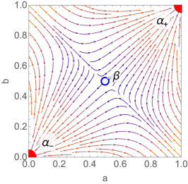
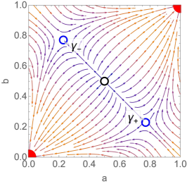
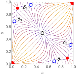
Figure 1: Flow field of the dynamical system defined by Eq. (1) for the cases: (a) $\epsilon=0.25$ (greater than $\epsilon^{c}=\frac{1}{5}$), (b) $\epsilon=0.15$ (between $\epsilon_{c}=\frac{1}{9}$ and $\epsilon^{c}$), and (c) $\epsilon=0.08$ (less than $\epsilon_{c}$). The arrow colors indicate the flow magnitude (blue slow, red fast) and the symbols indicate the locations of the fixed points: red dots for stable, blue circles for saddles, and black circle for unstable.

Consider now the HMR model for arbitrary $\epsilon\leq 1$. For simplicity, we analyze the symmetric situation with $N$ individuals in each class. Denote by $n_{\text{A}}$ and $n_{\text{B}}$ the number of A’s and B’s with opinion state $+1$. The densities of these two classes, $a=n_{\text{A}}/N$ and $b=n_{\text{B}}/N$, obey

$$\dot{a} =F(a)+\epsilon G(a,b)\,,\qquad\dot{b}=F(b)+\epsilon G(b,a)\,,$$ (1)

where

$$F(x) =x^{2}(1\!-\!x)-x(1\!-\!x)^{2}\,,$$

$$G(x,y) =(1\!-\!x)\big{[}2xy\!+\!y^{2}\big{]}\!-\!x\big{[}2(1\!-\!x)(1\!-\!y)\!+\!(1\!-\!y)^{2}\big{]}$$

(see the supplementary material for details). The dynamical behavior of the system (1) is quite rich, as illustrated by the flow field for generic values of $\epsilon$ in each of the three domains: (i) $\epsilon>\epsilon^{c}=\frac{1}{5}$; (ii) $\epsilon_{c}<\epsilon<\epsilon^{c}$ with $\epsilon_{c}=\frac{1}{9}$; (iii) $\epsilon<\epsilon_{c}$ (Fig. 1).

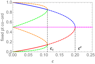
Figure 2: The coordinates of the fixed points as function of $\epsilon$, with dotted, dashed, and solid indicating unstable, saddle, and stable nodes, respectively. (magenta) The symmetric fixed point $\beta=\big{(}\frac{1}{2},\frac{1}{2}\big{)}$. (red/blue) The two reflection-symmetric fixed points $\gamma_{\pm}$ in the range $\epsilon=0$ to $\epsilon^{c}=\frac{1}{5}$. (green/orange) The four non-symmetric fixed points $\delta_{i}$ that emerge from $\gamma_{\pm}$ at $\epsilon_{c}=\frac{1}{9}$ and also extend to $\epsilon=0$. A single color gives the $x$ and $y$ coordinates of a given fixed point $\delta_{i}$.

When $\epsilon>\epsilon^{c}$, the consensus fixed points at $\alpha_{-}\equiv(0,0)$ and $\alpha_{+}\equiv(1,1)$ are stable nodes, while the fixed point $\beta\equiv\big{(}\frac{1}{2},\frac{1}{2}\big{)}$ is a saddle. From any initial condition that does not lie on the line $a+b=1$, the population quickly reaches consensus at $\alpha_{-}$ for $a+b<1$ and consensus at $\alpha_{+}$ for $a+b>1$. For initial conditions that lie on the line $a+b=1$, the population is driven to the fixed point $\beta$. However, stochastic finite $N$ fluctuations drive the system from this line (and even from the fixed point $\beta$ if the evolution begins there) and either consensus is reached with equal probabilities. We show below that the consensus time scales as $\ln N$ in all cases.

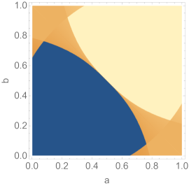
Figure 3: The basin of attraction to the consensus fixed point (0,0) (blue) and (1,1) (yellow) and to the mixed-opinion fixed points $\gamma_{\pm}$ (orange) for the case $\epsilon=0.1$.

In the intermediate regime, $\epsilon_{c}<\epsilon<\epsilon^{c}$, the fixed point $\beta$ changes from a saddle to an unstable node and two additional saddle-node fixed points

$$\gamma_{\pm}=\tfrac{1}{2}\left(1\pm\Gamma\,,1\mp\Gamma\right),\quad\Gamma=\sqrt{\frac{1-5\epsilon}{1-\epsilon}}\,,$$ (2)

emerge from $\beta$. These fixed points recede from $\beta$ as $\epsilon$ decreases below $\epsilon^{c}$ while remaining on the line $a+b=1$ (Fig. 2). According to the rate equations, if the initial condition lies on the line $a+b=1$, except for $(a,b)=\beta$, the population is drawn to one of the fixed points $\gamma_{\pm}$. At $\gamma_{+}$, for instance, a fraction $\frac{1}{2}(1+\Gamma)$ of A’s is in the $+1$ state, while the same majority of B’s is in the $-1$ state. Thus the total population is polarized but evenly balanced, with one-half in the $+1$ opinion state and the other half in the $-1$ state. All other initial conditions are again driven to consensus.

When $\epsilon<\epsilon_{c}$, four additional fixed points $\delta_{i}$ (i=1,2,3,4) emerge, two from $\gamma_{+}$ and two from $\gamma_{-}$. These four fixed points are saddle nodes, while the fixed points $\gamma_{\pm}$ become stable. There are now two disjoint domains in phase space that are attractors to one of these mixed-opinion fixed points $\gamma_{\pm}$ (Fig. 3). In this regime, the population-average interaction is sufficiently weak that A’s and B’s form their own and distinct near-consensus enclaves when the initial condition is within either of these basins of attraction for $\gamma_{+}$ or $\gamma_{-}$ (Fig. 1(c)). Again, the population is polarized but evenly balanced and there is range of initial conditions for which the population is driven to this polarized state. Initial conditions that lie outside these two basins of attraction are again quickly driven to one of the consensus fixed points.

Finite-Population Simulations. Even for a perfectly-mixed population, the rate equation approach does not fully capture the stochastic dynamics. Because of finite-$N$ fluctuations, the only true attractors of the dynamics are the consensus fixed points. If the population state is in the basin of attraction of one of the fixed points $\gamma_{\pm}$ (the situation pertinent for $\epsilon<\epsilon_{c}$), the dynamics first draws the population to one of these fixed points. Eventually, however, a sufficiently large stochastic fluctuation pushes the population out of these basins and to one of the consensus fixed points. The probability to leave either of these basins is exponentially small in $N$, which implies that the time to reach consensus grows exponentially with $N$. Even though consensus is the true final state of the population, reaching consensus requires a time that is practically unattainable for a population of any appreciable size. Thus for $\epsilon<\epsilon_{c}$, consensus is effectively not reached.

An analogous dichotomy occurs in population dynamics models, such as the logistic process, where the rate equation predicts a steady state, whereas extinction is the final outcome Karlin and McGregor (1964); Nåsell (2011); Allen (2015). In these processes, extinction occurs in a time that scales exponentially with the quasi steady-state population size predicted by the rate equation (see, e.g., Elgart and Kamenev (2004); Kessler and Shnerb (2007); Assaf and Meerson (2010, 2017)). The HMR model exhibits a similar rare-event driven approach to a final consensus, but with the additional feature that this approach is governed by two very different time scales.

In our simulations, we first select three individuals at random from the entire population. If these individuals are all from the same class, majority rule is applied. If the group consists of different classes of individuals, majority rule is applied with probability $\epsilon$; otherwise, nothing happens. The time is increment by $3/N$ in each update so that every individual reacts once, on average, in a single time unit. This update is repeated until consensus is achieved. We investigated several generic initial conditions: (a) A fully polarized state, with A’s are entirely in the $+1$ state, and B’s are entirely in the $-1$ state; (b) a “balanced” state, in which half of both the A’s and B’s are in the $+1$ state; (c) “imbalanced” states, in which a fraction $q$ of the A’s and a fraction $1-q$ of the B’s are in the $+1$ state. This initial condition lies along the line $a+b=1$ in state space. The results for these initial conditions are qualitatively similar and we primarily focus on the balanced initial condition.

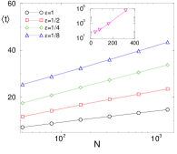
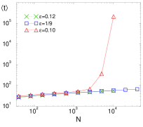
Figure 4: The average consensus time $\langle t\rangle$ versus $N$ for the balanced initial condition for: (a) a range of $\epsilon$ values and (b) close to the transition at $\epsilon=\epsilon_{c}$. In (a), the abscissa is on a logarithmic scale in the main panel and the ordinate is on a logarithmic scale in the inset, where data for the case $\epsilon=\frac{1}{16}$ is shown.

For $\epsilon>\epsilon_{c}$, the average consensus time $\langle t\rangle$ grows logarithmically with $N$. This is an exact result Krapivsky and Redner (2003) for the original MR model ($\epsilon=1$), and it is also proved to occur for majority-like stochastic processes that are described by rate equations that possess only saddles and sinks—escaping a saddle and reaching a sink takes $O(\ln N)$ time Schoenebeck and Yu (2018, 2020). This logarithmic dependence also occurs in the regime $\epsilon_{c}\leq\epsilon\leq\epsilon^{c}$. In this intermediate regime, when the initial state is on the line $a+b=1$, finite-$N$ fluctuations will drive the population state off this line (where $\gamma_{\pm}$ are attractors), after which consensus is quickly reached.

When $\epsilon$ decreases below $\epsilon_{c}=\frac{1}{9}$, the $N$ dependence of $\langle t\rangle$ suddenly changes from logarithmic to exponential (Fig. 4(b)). Strikingly, this exponential dependence sets in only after $N\gtrsim 4000$ for the case $\epsilon=0.1$, a feature that arises from from the geometry of the basin of attraction (Fig. 3(b)). To reach one of the fixed points $\gamma_{\pm}$ when starting from $(a,b)=(\frac{1}{2},\frac{1}{2})$, the population state has to navigate within the tongue between the separatrices that border the basins of attraction to $\gamma_{\pm}$. This tongue is narrow when $\epsilon$ is close to $\epsilon_{c}$, so the population state is typically and quickly drawn to a consensus fixed point in this range. However, if either fixed point $\gamma_{\pm}$ is reached, the escape time scales exponentially with $N$. These two outcomes explain the existence of two drastically different time scales in $P(t)$, the consensus-time distribution (Fig. 5). We may estimate the probabilities of the two outcomes from the data for $P(t)$ and find that the probability to reach one of the fixed points $\gamma_{\pm}$ vanishes as $\epsilon\to\epsilon_{c}$ from below; a bound for this probability is given in the supplemental material. Finally, note that this bimodal consensus-time distribution (Fig. 5) arises when the starting state is $(a,b)=(\frac{1}{2},\frac{1}{2})$. If the starting point lies inside the basin of attraction of $\gamma_{\pm}$, the consensus-time distribution is asymptotically exponential, $P(t)=\langle t\rangle^{-1}e^{-t/\langle t\rangle}$ and is fully characterized by the average consensus time Assaf and Meerson (2017).

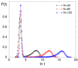
Figure 5: The consensus-time distribution for the balanced initial condition when $\epsilon=0.03$ for $N=40$, 80 and 120.

Deep in the ultra-slow regime, these two disparate time scales can be readily quantified. For example, for $\epsilon=0.03$, the average consensus time $\langle t\rangle$ over $10^{5}$ realizations is approximately $1304,~{}57104,~{}2,477,250$ for $N=40,~{}80,~{}120$. However, the underlying distribution of consensus times consists of two widely separated peaks (Fig. 5). These peaks are located at roughly $t\approx 23.8$ and $3.3\times 10^{3}$ for $N=40$, $t\approx 29$ and $1.6\times 10^{5}$ for $N=80$, and $t\approx 33$ and $8.9\times 10^{6}$ for $N=120$. The smaller of these two times grows close to logarithmically with $N$, while the larger time grows roughly exponentially with $N$. Thus the average consensus time is not a useful measure of how long it takes a given realization of the population to reach consensus.

To appreciate the dynamical source of these disparate time scales for $\epsilon<\epsilon_{c}$, it is useful to trace individual state-space trajectories. Figure 6 shows two such trajectories for $\epsilon=0.03$ and $N=80$. One (magenta) corresponds to quick consensus, in which the trajectory moves quasi-systematically from the initial state of $(a,b)=(\frac{1}{2},\frac{1}{2})$ to consensus at (0,0) in a time of roughly $29.5$. The other trajectory (multiple colors) shows ultra-slow approach to consensus. The blue portion shows the first 100 steps, where the population state quickly goes from $(\frac{1}{2},\frac{1}{2})$ to a metastable state near the fixed point $\gamma_{+}\approx(0.968,0.032)$. The green portion shows the trajectory in the time range between $t\approx 100$ and $0.999\,T$, where $T=126,456$ is the consensus time for this trajectory. This part of the trajectory wanders stochastically about the fixed point $\gamma_{+}$ until a large fluctuation drives this trajectory outside the local basin of attraction, after which the consensus fixed point at $(1,1)$ is reached (red portion of the trajectory).

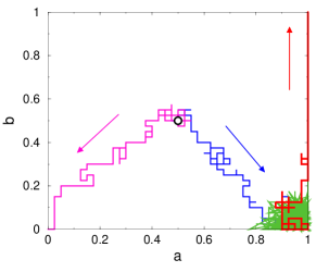
Figure 6: Two representative state-space trajectories for $\epsilon=0.03$ and $N=80$ that both start from $(\frac{1}{2},\frac{1}{2})$: (magenta) a trajectory that quickly goes to consensus at $(0,0)$; (blue/green/red) a trajectory that quickly reaches a metastable state near the fixed point $\gamma_{+}$ before eventually reaching consensus.

When $\epsilon=\epsilon_{c}$, the boundary between the logarithmic and exponential dependence of the average consensus time, we might have anticipated‘q that $\langle t\rangle$ would scale algebraically with $N$. However, simulations indicate logarithmic scaling at $\epsilon=\epsilon_{c}$ (Fig. 4(b)). We also might have anticipated that the consensus time is an asymptotically non-self-averaging random quantity in the intermediate regime $\epsilon_{c}\leq\epsilon\leq\epsilon^{c}$ because of the presence of the fixed points $\gamma_{\pm}$. However, simulations suggest that the consensus time is self-averaging for all $\epsilon\geq\epsilon_{c}$. Specifically, we found that the fluctuation measure $R\equiv\sqrt{\langle t^{2}\rangle}/\langle t\rangle\to 1$ faster than algebraically in $N$ when $\epsilon>\epsilon^{c}$, and as $N^{-1/2}$ when $\epsilon=\epsilon_{c}$. Thus we conclude that the consensus time $t$ is a self-averaging random quantity that scales as $\ln N$ for all $\epsilon\geq\epsilon_{c}$.

Majority rule dynamics in a two-class population favors quick consensus (logarithmic in population size) when individuals heed members of the other class with probability greater than 11%. Otherwise, a polarized state occurs for appropriate initial conditions. In a polarized state, one class strongly prefers the $+1$ opinion state and the other class prefers the $-1$ state, even though neither class has an internal preference for a given opinion. This polarized state is practically eternal in that the escape time to reach consensus scales exponentially with population size. Such freezing in of polarization seems characteristic of the current political climate Adamic and Glance (2005); Wang et al. (2017); Wang and Luo (2018); Baumann et al. (2021) and illustrates the crucial role of interactions between different classes of individuals in fostering either camaraderie or animosity. Our work also raises many interesting challenges, such as understanding homophilous majority rule on more realistic or dynamically evolving networks, heterogeneous groupings, and more than two opinion states.

We thank Mauro Mobilia for helpful suggestions and manuscript comments. SR was partially supported by NSF grant DMR-1910736.

I Rate Equations

We derive rate equations that provide the deterministic description of the evolution of the homophilous majority-rule (HMR) model. We start with the simplest case of $\epsilon=1$ when the type of the individual does not influence the behavior. We thus focus on the time evolution of individuals with a given opinion. The density $\rho(t)$ of individuals with opinion $+1$ evolves according to

$$\dot{\rho}=F(\rho),\qquad F(\rho)=\rho^{2}(1-\rho)-\rho(1-\rho)^{2}\,.$$ (S1)

The gain term account fir a group that consists of two individuals with opinion $+1$ and one individual with opinion $-1$; the loss term accounts for a group of the opposite composition. The time unit is chosen in such way that each individual is potentially updated once per unit time.

For the general HMR model, we denote by $a$ and $b$ the densities of individuals of type A and B that are in the $+1$ opinion state. Possible states in a group of three individuals can be obtained by expanding the multinomial $(A_{+}+A_{-}+B_{+}+B_{-})^{3}$, where the subscripts denote the opinion state of a given individual. For example, the state $A_{+}A_{-}B_{+}$ (with multiplicity 6) corresponds a heterogeneous group in the opinion state $++-$. When majority rule is applied, this group will go to the opinion state $+++$ with probability $6\epsilon a(1-a)b$. All the other terms in the multinomial expansion can be explained similarly. As a result of this enumeration of all states, the time dependence of the densities $a$ and $b$ are given by the rate equations

$$\dot{a}=F(a)+\epsilon G(a,b),\qquad\dot{b}=F(b)+\epsilon G(b,a)\,,$$ (S2)

with $F(x)$ defined in (S1) and

$$G(x,y)=(1-x)\big{[}2xy+y^{2}\big{]}-x\big{[}2(1-x)(1-y)+(1-y)^{2}\big{]}\,.$$ (S3)

Equations (S2) reduce to (S1) when $\epsilon=0$. In this extreme limit of the HMR model, individuals of type A and B do not “talk” to each other, so an individual is potentially updated only if the two other members of the group are of the same type. Therefore the overall rate is four times smaller than the rate used in (S1) and the rate equations would be $\dot{a}=\frac{1}{4}F(a)$ and $\dot{b}=\frac{1}{4}F(b)$ in the units of time used in (S1). The choice of time units in (S2) is made on aesthetic grounds to eliminate prefactors. As another consistency check, we set $\epsilon=1$ when individuals are “blind” and react independently on the type. Summing Eqs. (1) gives $\rho=(a+b)/2$ satisfies $\dot{\rho}=4F(\rho)$, with the factor of four reflecting the different choice of time in units in (S1) and (S2).

II Fixed Points

The flow field associated with the dynamical system defined by Eqs. (S2) and (S3) are displayed in Fig. 1 of the main text for representative values of $\epsilon$ in each of the three distinct domains of behavior: (a) $\epsilon>\epsilon^{c}$, with $\epsilon^{c}=\frac{1}{5}$, (b) $\epsilon$ between $\epsilon_{c}$ and $\epsilon^{c}$, with $\epsilon_{c}=\frac{1}{9}$ and (c) $\epsilon<\epsilon_{c}$. These flow fields were obtained by using the StreamPlot function in Mathematica.

For $\epsilon>\epsilon^{c}$, there are three trivial fixed points that are located at

$$(0,0),\qquad\big{(}\tfrac{1}{2},\tfrac{1}{2}\big{)},\qquad(1,1).$$ (S4)

These fixed points exist for all values of $\epsilon$ in the range $[0,1]$. The fixed points $(0,0)$ and $(1,1)$ are always stable and correspond to the consensus states. The symmetric fixed point $\big{(}\tfrac{1}{2},\tfrac{1}{2}\big{)}$ is a saddle node for this range of $\epsilon$ and it corresponds to a balanced and polarized state in which half the A’s and half the B’s in the population are in each opinion state. If the initial condition is not on the co-diagonal $a+b=1$, the dynamics quickly drives the population to one of the consensus states (Fig. 1(a)). If, however, the initial condition lies on the co-diagonal $a+b=1$ (with neither $a=1$ or $b=1$), rate equations predict that the population slowly approaches the symmetric fixed point $\big{(}\tfrac{1}{2},\tfrac{1}{2}\big{)}$.

For intermediate values of $\epsilon$ that lie between $\epsilon_{c}$ and $\epsilon^{c}$, in addition to the fixed points (S4), two new fixed points emerge. These fixed points are symmetrically located on the co-diagonal $a+b=1$ at

$$\gamma_{\pm}=\frac{1}{2}\left(1\pm\Gamma\,,1\mp\Gamma\right),\qquad\Gamma(\epsilon)=\sqrt{\frac{1-5\epsilon}{1-\epsilon}}\,,$$ (S5)

see Fig. 1(b). For values of $\epsilon$ in this intermediate range, the symmetric fixed point is now unstable and the new fixed points $\gamma_{\pm}$ are saddle nodes. If the initial densities are not on the co-diagonal $a+b=1$, the population again quickly approaches one of the consensus fixed points. If the initial densities are on the co-diagonal $a+b=1$ (except at $(\frac{1}{2},\frac{1}{2})$), then the population approaches one of the fixed points $\gamma_{\pm}$. If the initial densities are $(\frac{1}{2},\frac{1}{2})$, the population remains at this fixed point.

Finally, for $\epsilon<\epsilon_{c}$, the fixed points $\gamma_{\pm}$ become stable attractors and four new saddle nodes $\delta_{i}$ emerge ($i=1,2,3,4$) that are symmetrically located about $a+b=1$ (Fig. 1(c)). We order these fixed points by the magnitude of their vertical coordinates. There now exists two basins of attraction, one in the SE corner and one in the NW corner of the phase space $\{(a,b)\in[0,1]^{2}\}$ of the system for the fixed points $\gamma_{\pm}$ (Fig. 1(d)). Points outside these basins are attracted to one of the consensus fixed points. The basin boundaries are the separatrices from $\big{(}\tfrac{1}{2},\tfrac{1}{2}\big{)}$ to each $\delta_{i}$ and also from four specific points on the boundary of the phase space to $\delta_{1}$. Points on these separatrices are attracted to one of the $\delta_{i}$, apart from the symmetric fixed point $\big{(}\tfrac{1}{2},\tfrac{1}{2}\big{)}$. When $\epsilon\to 0$, the stable fixed points $\gamma_{\pm}$ approach (0,1) and (1,0), and the saddle nodes $\delta_{i}$ approach $(\frac{1}{2},0)$, $(0,\frac{1}{2})$, $(1,\frac{1}{2})$, and $(\frac{1}{2},1)$. In the case of $\epsilon=0$, the full system breaks into two independent subpopulations that consists of only A and only B that each undergo pure majority-rule dynamics.

The location of the fixed points (S4) are obvious and the locations of the fixed points $\gamma_{\pm}$ can be determined by hand without too much difficulty. The determination of the locations of the fixed points $\delta_{i}$ are complicated and we use Mathematica for the computations that follow. The symmetry of the problem allows us to express locations of these fixed points $\delta_{i}=(x_{i},y_{i})$ through the coordinates of one fixed point:

$$\delta_{1}=(x_{1},y_{1}),\quad\delta_{2}=(1-y_{1},1-x_{1}),\quad\delta_{3}=(y_{1},x_{1}),\quad\delta_{4}=(1-x_{1},1-y_{1})$$ (S6)

We have chosen [Fig. 1(c)] as $\delta_{1}$ the fixed point with the smallest vertical coordinate, and ordered the other fixed points by the magnitude of the vertical component. The expressions for $x_{1},y_{1}$ are rather cumbersome and we find

$$2x_{1}=1+\sqrt{1-\frac{1+3\epsilon}{2}\left[\frac{1-3\epsilon}{1-\epsilon}+\sqrt{\frac{1-9\epsilon}{1-\epsilon}}\right]}$$ (S7)

The dependences of the fixed point locations on $\epsilon$ and their stability as a function of $\epsilon$ are shown in Fig. 2 in the main text.

To determine the stability of the fixed points, we need to evaluate the Jacobian matrix

$$J =\left(\begin{array}[]{cc}{\displaystyle\frac{\partial[F(a)+\epsilon G(a,b)]}{\partial a}}&{\displaystyle\frac{\partial[F(a)+\epsilon G(a,b)]}{\partial b}}\\[11.38109pt] {\displaystyle\frac{\partial[F(b)+\epsilon G(b,a)]}{\partial a}}&{\displaystyle\frac{\partial[F(b)+\epsilon G(b,a)]}{\partial b}}\\ \end{array}\right)~{}.$$ (S10)

Using the definitions (S1) and (S3) for $F$ and $G$, we have

$$\frac{\partial[F(a)+\epsilon G(a,b)]}{\partial a} =6a-6a^{2}-1+\epsilon\big{[}4a+6b-8ab-2b^{2}-3\big{]},$$

$$\frac{\partial[F(a)+\epsilon G(a,b)]}{\partial b} =2\epsilon\big{[}a(2-a-b)+(1-a)(a+b)\big{]},$$

$$\frac{\partial[F(b)+\epsilon G(b,a)]}{\partial a} =2\epsilon\big{[}b(2-a-b)+(1-b)(a+b)\big{]},$$

$$\frac{\partial[F(b)+\epsilon G(b,a)]}{\partial b} =6b-6b^{2}-1+\epsilon\big{[}4b+6a-8ab-2a^{2}-3\big{]}\,,$$

at each fixed point: The eigenvalues of the Jacobian evaluated at each fixed point determine its stability.

At the consensus fixed points, the Jacobian is diagonal, $J=\text{diag}[-1-3\epsilon,-1-3\epsilon]$, so the eigenvalues are negative, $\lambda_{1}=\lambda_{2}=-1-3\epsilon$, and both consensus fixed points are stable. At the symmetric fixed point $\big{(}\tfrac{1}{2},\tfrac{1}{2}\big{)}$, the Jacobian matrix and its corresponding eigenvalues are

$$J =\left(\begin{array}[]{cc}{\frac{1}{2}\displaystyle(1-\epsilon)}&{\displaystyle 2\epsilon}\\[11.38109pt] {\displaystyle 2\epsilon}&{\frac{1}{2}\displaystyle(1-\epsilon)}\end{array}\right)\,,\qquad\qquad\lambda_{1}=\tfrac{1}{2}(1+3\epsilon)\,,\qquad\lambda_{2}=\tfrac{1}{2}(1-5\epsilon)\,.$$ (S13)

These eigenvalues [Fig. S1(a)] vary linearly with $\epsilon$. One eigenvalue is always positive and the second is positive when $\epsilon<\epsilon^{c}=\frac{1}{5}$, so that the symmetric fixed point is unstable in this range. The second eigenvalue is negative when $\epsilon^{c}<\epsilon$, which implies that the symmetric fixed point is a saddle node in this range.

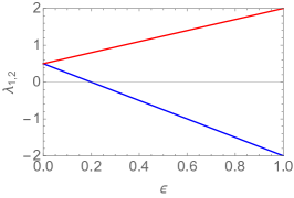
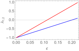
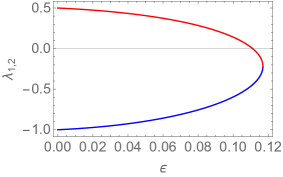
Figure S1: The $\epsilon$ dependence of the eigenvalues of the Jacobian matrix at: (a) the symmetric fixed point $\big{(}\tfrac{1}{2},\tfrac{1}{2}\big{)}$ in the range $0\leq\epsilon\leq 1$; (b) the fixed points $\gamma_{\pm}$ in the range $\epsilon\leq\epsilon^{c}=\frac{1}{5}$ where these fixed points exist; (c) the fixed points $\delta_{i}$ in the range $\epsilon\leq\epsilon_{c}=\frac{1}{9}$ where these fixed points exist.

At the reflection-symmetric fixed points $\gamma_{\pm}$, the Jacobian matrix and its corresponding eigenvalues are

$$J =\left(\begin{array}[]{cc}{\displaystyle-1+7\epsilon}&{\displaystyle 2\epsilon}\\[11.38109pt] {\displaystyle 2\epsilon}&{\displaystyle-1+7\epsilon}\end{array}\right)\,,\qquad\qquad\lambda_{1}=-1+9\epsilon\,,\qquad\lambda_{2}=-1+5\epsilon\,.$$ (S16)

The dependence of these eigenvalues on $\epsilon$ is shown in Fig. S1(b). The displayed range of the mixing parameter is $\epsilon<\epsilon^{c}=\frac{1}{5}$, where the fixed points $\gamma_{\pm}$ actually exist. One eigenvalue is positive and the other is negative for $\epsilon>\epsilon_{c}$, which means that these two fixed points are saddle nodes in this range. For $\epsilon<\epsilon_{c}=\frac{1}{9}$, both eigenvalues are negative, so that the fixed points $\gamma_{\pm}$ are stable nodes in this range. This change in behavior is reflected in the qualitative change in the flow field between Figs. 1(b) and 1(c).

At the four non-symmetric fixed points $\delta_{i}$, the expressions for the associated eigenvalues are extremely cumbersome. The Mathematica expressions for these eigenvalues and related information about the rate equation solution are available on the SR’s publications webpage (http://tuvalu.santafe.edu/~redner/pubs.html). The essential feature is that the eigenvalue $\lambda_{1}$ is positive and $\lambda_{2}$ is negative in the entire range $\epsilon<\epsilon_{c}$. The relevant range for this figure is $\epsilon<\epsilon_{c}=\frac{1}{9}$, where the fixed points $\delta_{i}$ actually exist. Thus each of the fixed points $\delta_{i}$ is a saddle node for all $0<\epsilon<\epsilon_{c}$.

III Fate of the balanced system for $\epsilon<\epsilon_{c}$

The balanced state $\big{(}\tfrac{1}{2},\tfrac{1}{2}\big{)}$ is a fixed point of the deterministic rate equations, but not of the actual stochastic HMR model. When $\epsilon\geq\epsilon_{c}$, the HMR model with the initial condition $(a,b)=\big{(}\tfrac{1}{2},\tfrac{1}{2}\big{)}$ quickly reaches one of the two consensus states. When $\epsilon<\epsilon_{c}$, however, fluctuations may drive the system into the basin of attraction of one of the stable fixed points $\gamma_{\pm}$. Indeed, when the population size is sufficiently large, the dynamics will be effectively deterministic, which allows us to make a simple estimate for the probability to reach the fixed point $\gamma_{+}$.

While we do not know the exact location of the separatrices analytically, Fig. 1(c) shows that the separatrices lie inside the wedge formed by the two rays that emanate from $\big{(}\tfrac{1}{2},\tfrac{1}{2}\big{)}$ to $\delta_{1}$ and to $\delta_{2}$. The angle $\theta$ between these rays therefore equals the angle between vectors $\big{(}x_{1}-\frac{1}{2},y_{1}-\frac{1}{2}\big{)}$ and $\big{(}\frac{1}{2}-y_{1},\frac{1}{2}-x_{1}\big{)}$. Thus an upper bound for probability $\Pi(\epsilon)$ that the state of the system enters the basin of attraction of $\gamma_{+}$ is

$$\Pi(\epsilon)\leq\frac{\theta}{\pi}=\frac{1}{\pi}\cos^{-1}\!\left[\frac{2\big{(}x_{1}-\frac{1}{2}\big{)}\big{(}\frac{1}{2}-y_{1}\big{)}}{\big{(}x_{1}-\frac{1}{2}\big{)}^{2}+\big{(}\frac{1}{2}-y_{1}\big{)}^{2}}\right]\,.$$ (S17)

After substituting the cumbersome expression for $x_{1}$ and $y_{1}$ from Eq. (S7) into (S17), we obtain a rather simple expression for the upper bound:

$$\Pi(\epsilon)\leq\frac{1}{\pi}\cos^{-1}\!\left[\frac{8\epsilon}{1-2\epsilon+9\epsilon^{2}}\right]\,.$$ (S18)

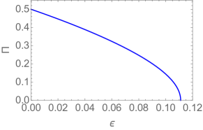
Figure S2: The $\epsilon$ dependence of Eq. (S18) for $\Pi(\epsilon)$, the probability for the system to enter the basin of attraction of the fixed point $\gamma_{+}$.

The behavior of this bound for the probability $\Pi(\epsilon)$ is shown in Fig. S2. In the limiting case of $\epsilon=0$, the upper bound (S18) gives $\frac{1}{2}$ which is exact. Indeed, for this case, individuals of type A and B do not interact, so that there are four possible consensus states $(0,0),~{}(1,0),~{}(0,1),~{}(1,1)$, each of which are reached equiprobably when the starting state is $(a,b)=\big{(}\tfrac{1}{2},\tfrac{1}{2}\big{)}$. Thus the probability $\Pi(0)$ to reach the $(1,0)$ or the $(0,1)$ consensus state is $\frac{1}{2}$.

IV Exponential HMR Model

According to the update rules of the HMR, the opinion change event $A_{+}\to A_{-}$ occurs in the following situations:

1. $A_{+}A_{-}A_{-}\longrightarrow A_{-}A_{-}A_{-}$  rate 1;

2. $A_{+}A_{-}B_{-}\longrightarrow A_{-}A_{-}B_{-}$  rate $\epsilon$;

3. $A_{+}B_{-}B_{-}\longrightarrow A_{-}B_{-}B_{-}$  rate $\epsilon$.

For the latter two cases, the opinion change $A_{+}\to A_{-}$ occurs at the same rate $\epsilon$ when the group opinion state is $--+$, as long as at least one of the individuals in the group is a B.

A natural alternative is that a person is motivated to change opinion by an individual from the same class with weight 1 and by an individual from the opposite class with weight $\epsilon$. This motivates the following modification of majority rule:

1. $A_{+}A_{-}A_{-}\longrightarrow A_{-}A_{-}A_{-}$  rate 1;

2. $A_{+}A_{-}B_{-}\longrightarrow A_{-}A_{-}B_{-}$  rate $\epsilon$;

3. $A_{+}B_{-}B_{-}\longrightarrow A_{-}B_{-}B_{-}$  rate $\epsilon^{2}$.

The qualitative behaviors of the original and this exponential version of HMR are essentially identical, so in the main text we investigated only the original version. For completeness, we outline the dynamical behavior of this exponential HMR.

The rate equations that govern the evolution of this exponential HMR model are

$$\dot{a}=F(a)+H(a,b),\qquad\dot{b}=F(b)+H(b,a),$$ (S19)

with the same $F(x)$ as in (S1), and

$$H(x,y)=2\epsilon x(1-x)(2y-1)+\epsilon^{2}\big{[}(1-x)y^{2}-x(1-y)^{2}\big{]}\,.$$ (S20)

The critical values of the mixing parameter are now

$$\epsilon^{c}=\frac{1}{3}\,,\qquad\epsilon_{c}=\sqrt{5}-2$$ (S21)

In addition to the trivial fixed points (S4), two additional fixed points $\gamma_{\pm}$ that are located at

$$\gamma_{\pm}=\tfrac{1}{2}\left(1\pm\Gamma\,,1\mp\Gamma\right),\qquad\Gamma=\frac{\sqrt{(1+\epsilon)(1-3\epsilon)}}{1-\epsilon}\,,$$ (S22)

emerge from $\beta$ when $\epsilon<\epsilon^{c}$. Four additional fixed points emerge from $\gamma_{\pm}$ at $\epsilon=\epsilon_{c}$ and the analog of (S7) is

$$2x_{1}=1+\frac{\sqrt{1-\epsilon+3\epsilon^{2}+\epsilon^{3}-(1+\epsilon)\sqrt{(1-\epsilon^{2})(1-4\epsilon-\epsilon^{2})}}}{\sqrt{2(1-\epsilon)}}~{}.$$ (S23)

In the $\epsilon\to 0$ limit, the density of A’s with opinion $-1$ in the polarized state $\gamma_{+}$ vanishes in a different manner in two versions:

$$a=\begin{cases}\epsilon+2\epsilon^{2}+5\epsilon^{3}+\ldots&\text{(HMR model)}\,,\\ \epsilon^{2}+2\epsilon^{3}+\ldots&\text{(exponential HMR)}\,.\end{cases}$$ (S24)

The primary new aspect of the exponential HMR model is that the polarized state becomes more extreme in character as $\epsilon\to 0$.

Finally, we note that in the $N\to\infty$ limit, the exponential HMR model can be interpreted as the standard MR model on a random graph that admits a partitioning into two complete sub-graphs of size $N$. Each subgraph represents one of the classes, either A and B, and any two nodes from different classes are connected with probability $\epsilon$.

References

- Castellano et al. (2009) C. Castellano, S. Fortunato, and V. Loreto, Rev. Mod. Phys. 81, 591 (2009).
- Galam (2012) S. Galam, Sociophysics: A Physicist’s Modeling of Psycho-political Phenomena (Springer, Berlin, 2012).
- Sznajd-Weron and Sznajd (2000) K. Sznajd-Weron and J. Sznajd, Int. J. Mod. Phys. C 11, 1157 (2000).
- Galesic and Stein (2019) M. Galesic and D. L. Stein, Physica A 519, 275 (2019).
- Clifford and Sudbury (1973) P. Clifford and A. Sudbury, Biometrika 60, 581 (1973).
- Holley and Liggett (1975) R. A. Holley and T. M. Liggett, Ann. Probab. 3, 643 (1975).
- Cox (1989) J. T. Cox, Ann. Probab. 17, 1333 (1989).
- Liggett (2013) T. M. Liggett, Stochastic Interacting Systems: Contact, Voter and Exclusion Processes, Vol. 324 (Springer Science & Business Media, 2013).
- Krapivsky (1992) P. L. Krapivsky, Phys. Rev. A 45, 1067 (1992).
- Frachebourg and Krapivsky (1996) L. Frachebourg and P. L. Krapivsky, Phys. Rev. E 53, R3009 (1996).
- Dornic et al. (2001) I. Dornic, H. Chaté, J. Chave, and H. Hinrichsen, Phys. Rev. Lett. 87, 045701 (2001).
- Krapivsky et al. (2010) P. L. Krapivsky, S. Redner, and E. Ben-Naim, A Kinetic View of Statistical Physics (Cambridge University Press, Cambridge, UK, 2010).
- Baronchelli (2018) A. Baronchelli, R. Soc. Open Sci. 5, 172189 (2018).
- Redner (2019) S. Redner, Comptes Rendus Physique 20, 275 (2019).
- Axelrod (1997) R. Axelrod, J. Conflict Resolution 41, 203 (1997).
- Axtell et al. (1996) R. Axtell, R. Axelrod, J. M. Epstein, and M. D. Cohen, Comput. Math. Organ. Theory 1, 123 (1996).
- Castellano et al. (2000) C. Castellano, M. Marsili, and A. Vespignani, Phys. Rev. Lett. 85, 3536 (2000).
- Vázquez and Redner (2007) F. Vázquez and S. Redner, EPL 78, 18002 (2007).
- Weisbuch et al. (2002) G. Weisbuch, G. Deffuant, F. Amblard, and J.-P. Nadal, Complexity 7, 55 (2002).
- Hegselmann and Krause (2002) R. Hegselmann and U. Krause, J. Artif. Soc. Social Simul. 5 (2002).
- Ben-Naim et al. (2003) E. Ben-Naim, P. L. Krapivsky, and S. Redner, Physica D: Nonlinear Phenomena 183, 190 (2003).
- Vazquez et al. (2003) F. Vazquez, P. L. Krapivsky, and S. Redner, J. Phys. A: Mathematical and General 36, L61 (2003).
- Marvel et al. (2012) S. A. Marvel, H. Hong, A. Papush, and S. H. Strogatz, Phys. Rev. Lett. 109, 118702 (2012).
- Mobilia (2011) M. Mobilia, EPL 95, 50002 (2011).
- Antal et al. (2005) T. Antal, P. L. Krapivsky, and S. Redner, Phys. Rev. E 72, 036121 (2005).
- Kułakowski et al. (2005) K. Kułakowski, P. Gawroński, and P. Gronek, Int. J. Mod. Phys. C 16, 707 (2005).
- Antal et al. (2006) T. Antal, P. L. Krapivsky, and S. Redner, Physica D 224, 130 (2006).
- Marvel et al. (2011) S. A. Marvel, J. Kleinberg, R. D. Kleinberg, and S. H. Strogatz, Proc. Natl. Acad. Sci. 108, 1771 (2011).
- Minh Pham et al. (2020) T. Minh Pham, I. Kondor, R. Hanel, and S. Thurner, J. R. Soc. Interface 17, 20200752 (2020).
- Galam (1999) S. Galam, Physica A 274, 132 (1999).
- Krapivsky and Redner (2003) P. L. Krapivsky and S. Redner, Phys. Rev. Lett. 90, 238701 (2003).
- Mobilia and Redner (2003) M. Mobilia and S. Redner, Phys. Rev. E 68, 046106 (2003).
- Crokidakis and de Oliveira (2015) N. Crokidakis and P. M. C. de Oliveira, Phys. Rev. E 92, 062122 (2015).
- Schoenebeck and Yu (2018) G. Schoenebeck and F.-Y. Yu, in Proceedings of the Twenty-Ninth Annual ACM-SIAM Symposium on Discrete Algorithms (SIAM, 2018) pp. 1945–1964.
- Mukhopadhyay et al. (2020) A. Mukhopadhyay, R. R. Mazumdar, and R. Roy, J. Stat. Phys. 181, 1239 (2020).
- Nguyen et al. (2020) V. X. Nguyen, G. Xiao, X. J. Xu, Q. Wu, and C.-Y. Xia, Sci. Report 10, 456 (2020).
- Schoenebeck and Yu (2020) G. Schoenebeck and F.-Y. Yu, in Proceedings of the 21st ACM Conference on Economics and Computation (2020) pp. 49–67.
- Noonan and Lambiotte (2021) J. Noonan and R. Lambiotte, arXiv:2101.03632 (2021).
- Chen and Redner (2005a) P. Chen and S. Redner, Phys. Rev. E 71, 036101 (2005a).
- Chen and Redner (2005b) P. Chen and S. Redner, J. Phys. A 38, 7239 (2005b).
- McPherson et al. (2001) M. McPherson, L. Smith-Lovin, and J. M. Cook, Ann. Rev. Sociol. 27, 415 (2001).
- Kossinets and Watts (2009) G. Kossinets and D. J. Watts, Am. J. Sociol. 115, 405 (2009).
- Barberá (2015) P. Barberá, Political Analysis 23, 76 (2015).
- Karlin and McGregor (1964) S. Karlin and J. McGregor, Stochastic Models in Medicine and Biology (Univ. Wisconsin Press, Madison, 1964).
- Nåsell (2011) I. Nåsell, Extinction and Quasi-stationarity in the Stochastic Logistic SIS Model (Springer, Berlin, 2011).
- Allen (2015) J. Allen, Stochastic Population and Epidemic Models — Persistence and Extinction (Springer, Berlin, 2015).
- Elgart and Kamenev (2004) V. Elgart and A. Kamenev, Phys. Rev. E 70, 041106 (2004).
- Kessler and Shnerb (2007) D. A. Kessler and N. M. Shnerb, J. Stat. Phys. 127, 861 (2007).
- Assaf and Meerson (2010) M. Assaf and B. Meerson, Phys. Rev. E 81, 021116 (2010).
- Assaf and Meerson (2017) M. Assaf and B. Meerson, J. Phys. A 50, 263001 (2017).
- Adamic and Glance (2005) L. A. Adamic and N. Glance, in Proceedings of the 3rd International Workshop on Link Discovery (2005) pp. 36–43.
- Wang et al. (2017) Y. Wang, J. Luo, and X. Zhang, in International Conference on Social Informatics (Springer, 2017) pp. 409–425.
- Wang and Luo (2018) Y. Wang and J. Luo, arXiv:1802.00156 (2018).
- Baumann et al. (2021) F. Baumann, P. Lorenz-Spreen, I. M. Sokolov, and M. Starnini, Phys. Rev. X 11, 011012 (2021).
Supplementary Material for Divergence and Consensus in Majority Rule
P. L. Krapivsky1 and S. Redner2
1Department of Physics, Boston University, Boston, MA, 02215 USA
2Santa Fe Institute, 1399 Hyde Park Road, Santa Fe, NM, 87501 USA