RNA Alternative Splicing Prediction with
Discrete Compositional Energy Network

Abstract.

A single gene can encode for different protein versions through a process called alternative splicing. Since proteins play major roles in cellular functions, aberrant splicing profiles can result in a variety of diseases, including cancers. Alternative splicing is determined by the gene’s primary sequence and other regulatory factors such as RNA-binding protein levels. With these as input, we formulate the prediction of RNA splicing as a regression task and build a new training dataset (CAPD) to benchmark learned models. We propose discrete compositional energy network (DCEN) which leverages the hierarchical relationships between splice sites, junctions and transcripts to approach this task. In the case of alternative splicing prediction, DCEN models mRNA transcript probabilities through its constituent splice junctions’ energy values. These transcript probabilities are subsequently mapped to relative abundance values of key nucleotides and trained with ground-truth experimental measurements. Through our experiments on CAPD, we show that DCEN outperforms baselines and ablation variants.

1. Introduction

RNA plays a key role in the human body and other organisms as a precursor of proteins. RNA alternative splicing (AS) is a process where a single gene may encode for more than one protein isoforms (or mRNA transcripts) by removing selected regions in the initial pre-mRNA sequence. In the human genome, up to 94% of genes undergo alternative splicing (Wang et al., 2008). AS not only serves as a regulatory mechanism for controlling levels of protein isoforms suitable for different tissue types but is also responsible for many biological states involved in disease (Tazi et al., 2009), cell development and differentiation (Gallego-Paez et al., 2017). While advances in RNA-sequencing technologies (Bryant et al., 2012) have made quantification of AS in patients’ tissues more accessible, an AS prediction model will alleviate the burden from experimental RNA profiling and open doors for more scalable in-silico studies of alternatively spliced genes.

Previous studies on AS prediction mostly either approach it as a classification task or study a subset of AS scenarios. Training models that can predict strengths of AS in a continuous range and are applicable for all AS cases across the genome would allow wider applications in studying AS and factors affecting this important biological mechanism. To this end, we propose AS prediction as a regression task and curate Context Augmented Psi Dataset (CAPD) to benchmark learned models. CAPD is constructed using high-quality transcript counts from the ARCHS4 database (Lachmann et al., 2018). The data in CAPD encompass genes from all 23 pairs of human chromosomes and include 14 tissue types. In this regression task, given inputs such as the gene sequence and an array of tissue-wide RNA regulatory factors, a model would predict, for key positions on the gene sequence, these positions’ relative abundance ($\psi$) in the mRNAs found in a patient’s tissue.

Each mRNA transcript may contain one or more splice junctions, locations where splicing occurred in the gene sequence. We hypothesize that a model design that considers these splice junctions would be key for good AS prediction. More specifically, these splice junctions are produced through a series of molecular processes during splicing, so modeling the energy involved at each junction may offer an avenue to model the whole AS process. This is the intuition behind our proposed discrete compositional energy network (DCEN) which models the energy of each splice junction, composes candidate mRNA transcripts’ energy values through their constituent splice junctions and predicts the transcript probabilities. The final component maps transcript probabilities to each known exon start and end’s $\psi$ values. DCEN is trained end-to-end in our experiments with ground-truth $\psi$ labels. Through our experiments on CAPD, DCEN outperforms other baselines that lack the hierarchical design to model relationships between splice site, junctions and transcript. To the best of our knowledge, DCEN is the first approach to model the AS process through this hierarchical design. While DCEN is evaluated on AS prediction here, it can potentially be used for other applications where the compositionality of objects (e.g., splice junctions/transcripts) applies. All in all, the prime contributions of our paper are as follows:

• We construct Context Augmented Psi Dataset (CAPD) to serve as a benchmark for machine learning models in alternative splicing (AS) prediction.

• To predict AS outcomes, we propose discrete compositional energy network (DCEN) to output $\psi$ by modeling transcript probabilities and energy levels through their constituent splice junctions.

• Through experiments on CAPD, we show that DCEN outperforms baselines and ablation variants in AS outcome prediction, generalizing to genes from withheld chromosomes and of much larger lengths.

2. Background: RNA Alternative Splicing

RNA alternative splicing (AS) is a process where a single gene (DNA / pre-mRNA) can produce multiple mRNAs, and consequently proteins, increasing the biodiversity of proteins encoded by the human genome. Pre-mRNAs contain two kinds of nucleotide segments, introns and exons. Each post-splicing mRNA transcript would only have a subset of exons while the introns and remaining exons are removed. A molecular machine called spliceosome joins the upstream exon’s end with the downstream exon’s start nucleotides to form a splice junction and removes the intronic segment between these two sites. In an example of an exon-skipping AS event in Figure 1, a single pre-mRNA molecule can be spliced into more than one possible mRNA transcripts ($T_{\alpha}$, $T_{\beta}$) with different probabilities ($P_{T_{\alpha}},P_{T_{\beta}}\in[0,1]$). These probabilities are largely determined by local features surrounding the splice sites (exon starts/ends) such as the presence of key motifs on the exonic and intronic regions surrounding the splice sites nucleotide. Global contextual regulatory factors such as RNA-binding proteins and small molecular signals (Witten and Ule, 2011; Boo and Kim, 2020; Taladriz-Sender et al., 2019) can also influence the transcript probabilities, creating variability for AS outcomes in cells from different tissue types or patients. While exon-skipping is the most common form of AS, there are others such as alternative exon start/end positions and intron retention.

2.1. Measurement of Alternative Splicing Outcome

One standard way to quantify AS outcome for a group of cells is through percent spliced-in ($\psi\in[0,1]$). Essentially, $\psi$ is defined as the ratio of relative abundance of an exon over all mRNA products within a single gene. An exon with $\psi=1$ means that it is included in all mRNAs found from experimental RNA-sequencing measurements while $\psi=0$ means the exon is missing in that particular gene. $\psi$ can also be annotated onto exon’s key positions such as its start and end locations. This allows one to approach the AS prediction as a regression task of predicting $\psi$ for each nucleotide of interest.

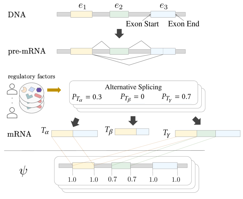
Figure 1. Mechanism of alternative splicing and its relationship with $\psi$ annotations. Introns in the gene sequences are colored gray while exons ($e_{1}$, $e_{2}$, $e_{3}$) are colored otherwise. Each patient sample has an unique set of regulatory factors, leading to a variety of alternative splicing outcomes in the population. In the training of DCEN, the DNA sequences of patients are assumed to be the same.

3. Related Work

We review prior art on RNA splicing prediction and energy-based models, highlighting those most similar to our work.

3.1. Splice Site Classification

The earliest task of machine learning on RNA splicing involves classification of splicing sites such as exon start and end positions in a given gene sequence, first using models such as decision trees (Pertea et al., 2001) and support vector machines (Degroeve et al., 2005). As deep learning gains wider adoption, a line of works uses neural networks for splice site prediction from raw sequence (Zuallaert et al., 2018; Zhang et al., 2018; Louadi et al., 2019; Jaganathan et al., 2019). In a recent example, (Jaganathan et al., 2019) used a 1-D Resnet model to classify individual nucleotides in a pre-mRNA sequence into 3 categories: 1) exon’s start, 2) exon’s end or 3) none of the two classes. Unlike these models that only classify splice sites, we propose DCEN to predict $\psi$ levels of splice sites which involve the consideration of patient-specific input such as levels of RNA regulatory factors on top of just primary gene sequences.

3.2. Alternative Splicing Prediction

The prior work in alternative splicing prediction can be categorized into two distinct groups. The first group framed the prediction as a classification task, whether an alternative splicing event would occur given input or change in input. The earliest examples involved using a Bayesian regression (Barash et al., 2010) and Bayesian neural network (Xiong et al., 2011) to predict whether an exon would be skipped or included in a transcript. (Leung et al., 2014) used a neural network with dense layers to predict the type of AS event. Using a classification framework (Xiong et al., 2015) to predict one of three classes (high/medium/low), the relative $\psi$ value can also be inferred. Another deep learning-based approach (Louadi et al., 2019) utilized a CNN-based framework to classify between four AS event classes (exon skipping, alternative 3’, alternative 5’ or constitutive exon).

The second group, which includes DCEN, addresses the prediction as a regression rather than a classification task. This formulation gives higher resolution in the AS event since predicted values correlate with the strength of the AS outcome. (Bretschneider et al., 2018) proposed a deep learning model to predict which site is most likely to be spliced given the raw sequence input of 80-nt around the site. The neural networks in (Cheng et al., 2019; Cheng et al., 2020) also use the primary sequences around candidate splice sites as inputs to infer their $\psi$ values. These approaches predict $\psi$ values of splice sites using only their individual representations without modeling the relationship between these splice sites and their parent transcripts, and are conceptually similar to the 2000-nt SpliceAI baseline here which is outperformed by DCEN in our experiments.

Since cellular signals such as RNA-binding proteins (RBPs) are observed to affect RNA splicing (Witten and Ule, 2011; Yee et al., 2019), models such as (Jha et al., 2017) predicts $\psi$ values with RBP information and generated genomic features used as input. while (Huang and Sanguinetti, 2017; Zhang et al., 2019) have emerged to incorporate both primary sequence features and RBP levels to better predict exon inclusion levels given a small number of experimental read counts. While also considering regulatory factors such as RBPs, our approach differs from (Witten and Ule, 2011; Yee et al., 2019) as we do not assume the availability of experimental read counts for the gene of interest. To the best of our knowledge, DCEN is the first approach to model whole transcript constructs (through energy levels) on top of the immediate neighborhood around the nucleotide of interest when predicting its $\psi$ value in the splicing process.

3.3. Energy-Based Models

Most recent work in energy-based models (EBM) (LeCun et al., 2006) focused on the application of image generative modeling. Neural networks were trained to assign low energy to real samples (Xie et al., 2016; Song and Ou, 2018; Du and Mordatch, 2019; Nijkamp et al., 2019; Grathwohl et al., 2019) so that realistic-looking samples can be sampled from the low-energy regions of the EBM’s energy landscape. Instead of synthesizing new samples, our goal here is to predict RNA splicing outcomes. Other applications of EBMs include anomaly detection (Song and Ou, 2018), protein conformation prediction (Du et al., 2020) and reinforcement learning (Haarnoja et al., 2017). Previous compositional EBMs such as (Haarnoja et al., 2017; Du et al., 2019) considered high dimensional continuous spaces in their applications which makes sampling from the model intractable. In contrast, since genes consist of a finite number of known transcripts, DCEN considers discrete space where the probabilities of the transcripts are tractable through importance sampling with a uniform distribution.

4. CAPD: Context Augmented Psi Dataset

The core aim of Context Augmented Psi Dataset (CAPD) is to construct matching pairs of sample-specific inputs and labels to frame the alternative splicing prediction as a regression task and facilitate future benchmarking of machine learning splicing prediction models. Each CAPD sample is a unique AS profile of a gene from the cells of a particular tissue type, from an individual patient. Its annotations contain $\psi\in[0,1]$ of all the know exon starts and ends for the particular gene. Apart from the $\psi$ labels, each data sample also contains the following as inputs: a) full sequence of the gene ($\operatorname{\mathbf{x}}$), b) nucleotide positions of all the known transcripts ($\mathcal{T}$) on the full gene sequence and c) levels of RNA-regulatory factors ($\operatorname{\mathbf{x}}_{\text{reg}}$).

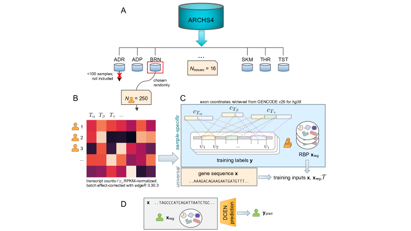
Figure 2. Pipeline of the CAPD dataset preparation with the steps as follows: A) a simple keyword search in the ARCHS4 v.8 database is performed to find a given number of samples for the specified tissues. Tissues for which the number of samples found is less than a specified threshold (N=100) are not included. B) Transcript libraries are normalized to RPKM, processing by edgeR library and outlier removal are performed. C) Normalized transcript counts are then used to construct training labels y and auxiliary regulatory vector inputs x_reg for each sample. The latter is then used together with pre-mRNA transcript sequence as model input. D) After model training, a sample input for $\psi$ prediction consists of pre-mRNA transcript sequence and a vector of abundance of sample-specific regulatory factors.

4.1. Construction of CAPD

We mine transcript abundance data from the publicly available ARCHS4 database v.8 (Lachmann et al., 2018). ARCHS4 database v.8 contains expression data for 238522 publicly available human RNA-seq samples that were retrieved from Gene Expression Omnibus (GEO) and aligned to human transcriptome Ensembl 90 cDNA (Zerbino, 2018) to produce count numbers for each transcript in each sample. A simple keyword search was used to find $250\times N_{T}$ samples for each of the 16 tissue types ($N_{T}=16$) selected for training: adipose tissue, blood, brain, breast, colon, heart, kidney, liver, lung, lymph node, prostate gland, skeletal muscle tissue, testes, thyroid gland. Underrepresented tissues, i.e. with the number of samples below a threshold ($N=100$) were not included (see the pipeline in Figure 2A). Each sample row contains transcript-centric raw RNA counts. Standard normalization of RNA read counts to RPKM (Mortazavi et al., 2008) was then performed. To exclude samples with significantly different expression patterns, a z-score outlier removal procedure described in (Oldham et al., 2008) for similar tasks was applied to samples from each tissue separately. Expression patterns of samples belonging to one tissue type are varying, and $\approx 2-5\%$ of the sample population is usually considered outlying by the algorithm. To homogenize the data, batch effects were removed with edgeR R library (Robinson et al., 2009) (Figure 2B). Heterogeneity of the data, however, is still expected as the samples belong to different sources and were chosen randomly. This gives the normalized transcript count values ($c_{T_{\alpha}}$) for each gene transcript ($T_{\alpha}$).

To construct the levels of RNA splicing regulatory factors ($\operatorname{\mathbf{x}}_{\text{reg}}$), we extract the expression levels of RBPs corresponding to the RBPDB database (Cook et al., 2011) and RNA chemically modifying corresponding to (Basturea, 2013) in a sample-wise manner from the normalized transcript count matrix (Figure 2C). This gives a 3971-dimensional $\operatorname{\mathbf{x}}_{\text{reg}}$. These, together with universal pre-mRNA transcript sequences (same for each sample), compose model input.

To generate primary pre-mRNA transcript sequences, we follow the procedure described in (Jaganathan et al., 2019): pre-mRNA (synonymous to DNA, with T $\to$ U) sequences are extracted with flanking ends of 1000 nt on each side, while intergenic sequences are discarded. Pseudogenes, genes with sequence assembly gaps and genes with paralogs are excluded from the data. Exon coordinate information is retrieved from GENCODE Release 26 for GRCh38 (Frankish et al., 2019) comprehensive set, downloaded from the UCSC table browser . We omit genes with missing matching GENCODE ID, resulting in a total of 19399 unique human gene sequences. The coordinates of the gene pre-mRNA sequence start and end are determined by the left- or right-most position among all the transcripts for that gene, further extended with flanking ends of 1000 nt for context on each side. The CAPD dataset is split into train and test according to the chromosome number and length of the genes. All genes in chromosome 1, 3, 5, 7, and 9 are withheld as test samples (Test-Chr), similar to (Jaganathan et al., 2019). To test that models can generalize to genes of longer lengths, we further withhold all genes from the other chromosomes that have $>$100K nt (Test-Long) and group them in the test set. The remaining genes are used for training. Key statistics of the CAPD is summarized in Table 1.

4.2. Label Annotation

The $\psi$ labels are constructed as follows (Figure 2C): 1) the count values $c_{i}$ for all known exon start and end (position $i$) are initialized to zero. 2) enumerating through all transcripts, each transcript count is added onto the counts of its constituent exons’ start/end $\mathbf{c}_{i}\leftarrow\mathbf{c}_{i}+c_{T_{m}},\forall i\in T_{m}$. 3) To compute $\psi$ values, each count value is divided by the sum of transcript counts to normalize its value to $[0,1]$, i.e., $\psi_{i}=\mathbf{c}_{i}/\sum_{m}c_{T_{m}}$ .

Table 1. CAPD data statistics.

	Train	Test-Chr	Test-Long
# of unique genes	11,472	5,604	2,323
mean pre-mRNA length (nt)	26,196	73,355	247,041
mean # of exons	6.7	7.0	10.5

5. DCEN: Discrete Compositional Energy Network

In § 2, we learn that final mRNA splice isoforms may comprise one or more splice junctions, points where upstream exon’s end and downstream exon’s start meet. Inspired by the creation of splice junctions by spliceosomes, the first stage of DCEN models the energy values of the splicing process at splice junctions. As the splice junctions are typically far enough ($\sim$300 nt) and assumed to be independent of one another, the energy of a final mRNA transcript can be composed by the summation of its constituent splice junctions’ energy. The second stage of DCEN derives probabilities for the formation of each transcript from their energy values. These transcript probabilities are then mapped to the relative abundance ($\psi$) of exon starts/ends at its corresponding splice sites. Since a particular splice junction may appear in more than one mRNA isoform, we design DCEN to be invariant to the splice junctions. In the following § 5.1, we discuss the key components of DCEN while § 5.5 details its training process.

5.1. Model Architecture

Here, we detail the DCEN learned energy functions and how transcript probabilities can be derived from their energy levels through Boltzmann distribution and importance sampling. A summary of DCEN model architecture is shown in Figure 3.

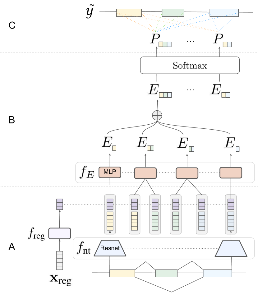
Figure 3. Model architecture of proposed discrete compositional energy network (DCEN). A) Learned representations of the DNA sequence are extracted by $f_{\text{nt}}$ while the representations of the regulatory factors by $f_{\text{reg}}$. B) The representation of a particular splice junction is the concatenation of acceptor and donor sites’ representations. The learned energy value of a particular splice junction is computed by passing its representation through $f_{E}$. The energy level of each transcript is the sum of its junctions’ energies. C) Through a softmax operation, the probability of each transcript in a gene is computed. By pooling the probabilities of all transcripts that contain a particular nucleotide, we get the nucleotide’s predicted $\psi$ value.

5.2. Learned Energy Functions

The weights of DCEN’s learned energy functions consist of a 1) feature extractor, 2) regulatory factors encoder and 3) junction energy network. The feature extractor ($f_{\text{nt}}$) takes the pre-mRNA sequence of length $l$ as its input ($\operatorname{\mathbf{x}}\in\mathbb{R}^{l\times 4}$) where 4 is the number of possible nucleotides and outputs a hidden representation ($\mathbf{h}_{\text{nt}}\in\mathbb{R}^{l\times d}$) for each nucleotide position ($\operatorname{\mathbf{x}}_{i}$) while the regulatory factors encoder ($f_{\text{reg}}$) takes in the levels of regulatory factors ($\operatorname{\mathbf{x}}_{\text{reg}}$) to compute a gene-wide hidden states $\mathbf{h}_{\text{reg}}\in\mathbb{R}^{d}$:

(1) $$\mathbf{h}_{\text{nt}}=f_{\text{nt}}(\operatorname{\mathbf{x}})~{},~{}~{}~{}~{}~{}\mathbf{h}_{\text{reg}}=f_{\text{reg}}(\operatorname{\mathbf{x}}_{\text{reg}})$$

We concatenate $\mathbf{h}_{\text{reg}}$ to all the position-specific $\mathbf{h}_{\text{nt}}$ to form a new position-wise hidden state ($\mathbf{h}_{i}$) that is dependent on regulatory factors. The representation of a particular splice junction ($J_{k}=(i,j)$) is the concatenation between the hidden states of upstream exon end’s and downstream exon start’s hidden states:

(2) $$\mathbf{h}_{J_{k}}=[\mathbf{h}_{i};\mathbf{h}_{j}]~{}~{},~{}~{}~{}~{}~{}\mathbf{h}_{i}=[\mathbf{h}_{\text{nt}_{i}};\mathbf{h}_{\text{reg}}]$$

If an exon start/end is the first/last nucleotide of a transcript, its hidden state is concatenated with a learned start/end token instead ($\mathbf{h}_{\text{start}}$ or $\mathbf{h}_{\text{end}}$ respectively). To model the energy ($E_{J_{k}}\in\mathbb{R}$) of producing splice junction $J_{k}$, we feed its representation into the energy network ($f_{E}$). We sum up the energy values of all splice junctions ($J_{k}$) inside a mRNA transcript ($T_{\alpha}$) to compose the total energy ($E_{T_{\alpha}}\in\mathbb{R}$) involved in producing the transcript from a splicing event:

(3) $$E_{T_{\alpha}}=\sum_{k}E_{J_{k}}~{}~{},~{}~{}~{}~{}~{}\forall J_{k}\in T_{\alpha}~{}~{},~{}~{}~{}~{}~{}E_{J_{k}}=f_{E}(\mathbf{h}_{J_{k}})$$

5.3. Transcript Probabilities from Energy Values

After obtaining the energy levels ($E_{T_{\alpha}}$) of all mRNA transcript candidates for a particular gene, we can compute the probabilities of these transcripts via a softmax operation through the theorem below.

Theorem 5.1.

Given the energy levels of all the possible discrete states of a system, the probability of a particular state $T_{i}$ is the softmax output of its energy $E_{T_{i}}$ with respect to those of all other possible states in the system, i.e.,

(4) $$P_{i}=\frac{\exp(-E_{T_{i}})}{\sum_{j}\exp(-E_{T_{j}})}=\mathrm{Softmax}_{i}(E)$$

Its proof, deferred to the Appendix § A.2, can be derived through Boltzmann distribution and importance sampling. Since each mRNA transcript $T_{\alpha}$ can be interpreted as a discrete state of the alternative splicing event for a particular gene (system) in Theorem 5.1, we can compute its probability from its energy value.

It is important to also consider a null state with energy $E_{\text{null}}$ where none of the gene’s mRNA transcripts is produced. In DCEN, $E_{\text{null}}$ is a learned parameter. In summary, the probability of producing transcript $T_{\alpha}$ in an gene splicing event is

(5) $$P_{T_{\alpha}}=\mathrm{Softmax}_{\alpha}(E)~{}~{},~{}~{}~{}~{}~{}E=[E_{T_{\alpha}},E_{T_{\beta}},\dots,E_{\text{null}}]$$

If the null state were not considered, the model would incorrectly assume that a particular gene is always transcribed since the sum of transcripts’ probabilities in a gene would be $\sum_{i}P_{T_{i}}=1$.

5.4. Exon Start/End Inclusion Levels from Transcript Probabilities

We can compute the probability of a particular (exon start/end) nucleotide of position $i$ by summing up the probabilities of all transcripts that contain that nucleotide.

(6) $$P_{i}=\sum_{m}P_{T_{m}}~{}~{},~{}~{}\forall T_{m}\in\mathcal{T}_{i}$$

where $\mathcal{T}_{i}$ is the set of transcripts containing the nucleotide of interest. By inferring the (exon start/end) nucleotide inclusion levels through transcript probabilities, our model has the advantage of additional access to the relative transcription level of the gene’s transcripts over baselines that infer directly at the nucleotide positions (such as baselines in § 6.1).

5.5. Training Algorithm

5.5.1. Regression Loss

Since experimental $\psi$ levels from CAPD are essentially the empirical observations of nucleotide present in the final mRNA transcript products, its normalized values ($y_{i}\in[0,1]$) can be used as the ground-truth label for the predicted nucleotide inclusion levels. This allows us to train DCEN as a regression task by minimizing the mean squared error (MSE) between the predicted nucleotide $\psi$ and the normalized experimental $\psi$ values:

(7) $$L_{\psi}=\sum_{i}\|\tilde{y_{i}}-y_{i}\|^{2}_{2}~{}~{},~{}~{}~{}~{}~{}\tilde{y_{i}}=P_{i}$$

In our experiments, only nucleotide positions that are either an exon start or end are involved in this regression training objective.

5.5.2. Classification Loss

We also include a classification objective, similar to (Jaganathan et al., 2019), where a classification head $f_{\text{cls}}$ takes the nucleotide hidden states ($\mathbf{h}_{\text{nt}}$) as input to predict probability of every nucleotide as one of the 3 classes (exon start, end and neither) to give the classification loss:

(8) $$L_{\text{cls}}=-\mathbf{y}_{\text{cls}}^{\top}\log f_{\text{cls}}(\mathbf{h}_{\text{nt}})$$

where $\mathbf{y}_{\text{cls}}$ is the ground-truth labels for each nucleotide. This helps the DCEN learn features on the gene primary sequence that are important for RNA splicing. A summary of the training phase is shown in Algorithm 1.

1

2Input: Training data $\mathcal{D}_{\text{train}}$, Learning rate $\gamma$,

3for  each training iteration  do

4       Sample $(\operatorname{\mathbf{x}},\operatorname{\mathbf{x}}_{reg},\mathbf{y},\mathcal{T},\mathcal{J})\sim\mathcal{D}_{\text{train}}$

5      $\mathbf{h}_{\text{nt}}\leftarrow f_{\text{nt}}(\operatorname{\mathbf{x}}),~{}~{}$

6      $L_{\text{cls}}\leftarrow-\mathbf{y}_{\text{cls}}^{\top}\log f_{\text{cls}}(\mathbf{h}_{\text{nt}})$ $\triangleright$ Compute exon start/end classification cross-entropy loss

7      $\mathbf{h}_{\text{reg}}\leftarrow f_{\text{reg}}(\operatorname{\mathbf{x}}_{reg})$

8      $\mathbf{h}_{i}\leftarrow[\mathbf{h}_{\text{nt}_{i}};\mathbf{h}_{\text{reg}}]~{}~{}$

9      $\mathbf{h}_{J_{k}}\leftarrow[\mathbf{h}_{i};\mathbf{h}_{j}]~{}~{},~{}~{}~{}$ $J_{k}=(i,j)~{}~{}$ $\triangleright$ Get junction state from upstream exon end $i$ and downstream exon start $j$

10      $E_{J_{k}}\leftarrow f_{E}(\mathbf{h}_{J_{k}})~{}~{}$ $\triangleright$ Compute splice junction energy

11      $E_{T_{\alpha}}\leftarrow\sum_{k}E_{J_{k}}~{}~{},~{}~{}\forall J_{k}\in T_{\alpha},~{}~{}\forall T_{\alpha}\in\mathcal{T}$ $\triangleright$ Compose transcript energy

12      $P_{T_{\alpha}}\leftarrow\mathrm{Softmax}_{\alpha}(E)~{}~{},~{}~{}E=[E_{T_{\alpha}},E_{T_{\beta}},\dots]$ $\triangleright$ Compute transcript probabilities

13      $\tilde{y_{i}}\leftarrow\sum_{m}P_{T_{m}}~{}~{},~{}~{}\forall T_{m}\in\mathcal{T}_{i}$

14      $L_{\psi}\leftarrow\sum_{i}\|\tilde{y_{i}}-y_{i}\|^{2}_{2}~{}~{}$ $\triangleright$ Compute exon start/end inclusion regression loss

15      $\theta\leftarrow\theta+\gamma~{}\nabla_{\theta}(\lambda_{\text{reg}}L_{\psi}+\lambda_{\text{cls}}L_{\text{cls}})$

Algorithm 1 Discrete Compositional Energy Network Training

6. Experiments

We evaluate DCEN and baselines on the prediction of the $\psi$ values of exon starts and ends in our new CAPD dataset. In the following, we describe the baseline models and DCEN ablation variants before discussing the experimental setup and how well these models generalize to withheld test samples.

6.1. Baselines and Ablation Variants

SpliceAI is a 1D convolutional Resnet (He et al., 2016) trained to predict splice sites on pre-mRNA sequences. We train three variants of SpliceAI to compare as baselines in our experiments: the first (SpliceAI-cls, Figure 4(a)) is trained only on the classification objective, similar to the original paper, to predict whether a nucleotide is an exon start, end or neither of them. The second (SpliceAI-reg, Figure 4(b)) is trained only on a regression objective like DCEN to directly predict the $\psi$ levels of nucleotides while the third variant (SpliceAI-cls+reg) is trained on both the classification and regression objectives. Both SpliceAI-reg and SpliceAI-cls+reg also have a regulatory factors encoder ($f_{\text{reg}}$) similar to DCEN’s to compute $\mathbf{h}_{i}$ and a regression head ($f_{\psi}$) to output $\psi$ level for each nucleotide. For a direct comparison, DCEN’s feature extractor $f_{\text{nt}}$ takes the same architecture as the SpliceAI Resnet. Two DCEN ablation variants are also evaluated: The Junction-psi model (Figure 4(c)) predicts the psi levels of a particular splice junction directly rather than its energy level in the case of DCEN. A simpler ablation variant (SpliceAI-ML or SpliceAI-match layers, Figure 4(b)) substitutes DCEN’s $f_{E}$ with a position-wise feedforward MLP containing the same number of parameters to verify that DCEN’s better performance is not due to more learned parameters.

6.2. Data & Models

We use the CAPD dataset (§ 4) for the training and evaluation of all models. 10% of the CAPD training genes are randomly selected as the validation set for early-stopping while the rest are used as training samples for the models. For DCEN’s $f_{\text{nt}}$ and the SpliceAI baselines, we follow the same setup as the SpliceAI-2K model in (Jaganathan et al., 2019) which is a Resnet made up of 1-D convolutional layers with a perceptive window of 2K nucleotides, 1K on each flanking sides. The SpliceAI Resnet model has a total of 12 residual units and hidden states of size 32. The number of channels in $\mathbf{h}_{\text{reg}}$ and $\mathbf{h}_{\text{nt}}$ are 32 while $\mathbf{h}$ has a size of 64 channels. We use a 3-layer MLP for $f_{\text{reg}}$. The regression head $f_{\psi}$ in SpliceAI-reg and SpliceAI-cls+reg is a 3-layer MLP with a sigmoid activation to outputs a scalar $\psi$ value. DCEN’s $f_{E}$ is a 4-layer MLP and outputs a scalar energy value for each splice junction. Intermediate hidden states of $f_{\text{reg}}$ and $f_{E}$ all have dimension of 32.

6.3. Training & Evaluation

All models are trained with Adam optimizer with a learning rate of 0.001 in our experiments. Due to the data’s large size, the training is early-stopped when the model’s validation performances plateau: less than 25% of the full train dataset for all models in our experiments. For the training of SpliceAI models, samples are fed into the model with a batch size of 8 sequences with a maximum length of 7K nucleotides (5K labeled + 2K flanking). For training of DCEN and its ablation variants, a SpliceAI-cls&reg model pretrained on CAPD was used as the weights of $f_{\text{reg}}$, $f_{\text{nt}}$ and only the parameters of $f_{E}$ is trained to reduce training time. In each training iteration of DCEN and its ablation variants, a batch of 16 genes was used to train the weights. We evaluate all the models on withheld test samples with two standard regression metrics: Spearman rank correlation and Pearson correlation. Pearson correlation measures the linear relationship between the ground-truth and predicted exon start/end inclusion levels while Spearman rank correlation is based on the ranked order of the prediction and ground-truth values.

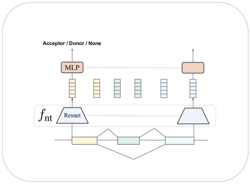
(a) SpliceAI-cls

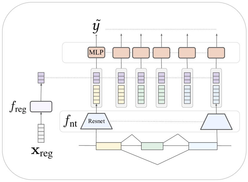
(b) SpliceAI-reg & -ML

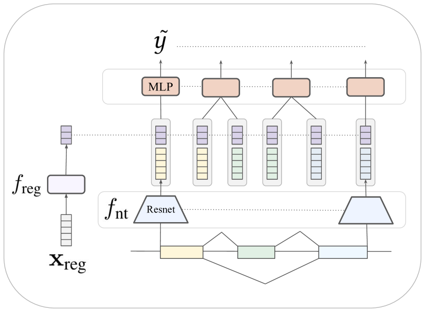
(c) Junction-psi

Figure 4. Ablation models used to compare with our proposed DCEN model. (a) SpliceAI-cls (Jaganathan et al., 2019) is trained to predict whether a particular nucleotide in the DNA sequence is an acceptor, donor site or neither of them from only the primary DNA sequence, without input of regulatory factors ($\operatorname{\mathbf{x}}_{reg}$). The predicted probability of the acceptor/donor class is assumed to be predicted $\psi$ values during the comparison. (b) SpliceAI-reg and SpliceAI-ML are both trained to predict the $\psi$ value of a particular nucleotide with a regression objective. These two ablation models, unlike DCEN (Figure 3), infer $\psi$ values from individual nucleotide’s representation and does not rely on the compositionality of transcripts and their splice junctions. (c) Junction-psi infers the $\psi$ value of a particular splice junction from the joint representations of its acceptor and donor sites, without modeling the relationship between junctions and their parent transcripts.

6.4. Results

The DCEN outperforms all baselines and ablation variants for both regression metrics when evaluated on the withheld test samples, as shown in Table 2. Even with the same number of parameters, the DCEN shows better performance than the SpliceAI-ML and Junction-psi model. Even with more trained parameters, Junction-psi model performs worse than the SpliceAI-reg and SpliceAI-cls+reg baselines while the SpliceAI-ML does not show clear improvement over these two baselines.

A key difference between these baselines and DCEN lies in DCEN’s inductive bias that models the hierarchical relationships between splice sites and junctions, as well as between splice junctions and their parent transcripts. Even with a matching number of parameters as DCEN, SpliceAI-ML still underperforms DCEN indicating DCEN’s model size is not the key contributor to its performance. These observations indicate that DCEN’s design to compose transcripts’ energy through splice junctions and infer their probabilities from energy values is key for better prediction. The correlation results reported in Table 2, 3 and 5 all have p-values of zero in working precision due to the large number of gene samples.

Training DCEN for 5 times the training steps at the early stopped point does not result in better (Table 6 in S A.1) nor much worse performance on the test samples. This suggests that DCEN is underfitting the training dataset and may benefit from a larger model size.

6.4.1. Excluded chromosomes

When evaluated separately test samples from chromosomes (1, 3, 5, 7, and 9) not seen during the training phase, DCEN maintains its superior performance (Table 3) when compared to the ablation baselines, showing that it generalizes across novel gene sequences.

Table 2. Performance of DCEN and baselines on all withheld test samples.

Model	Spearman Cor.	Pearson Cor.
SpliceAI-cls	0.399	0.349
SpliceAI-reg	0.579	0.574
SpliceAI-cls+reg	0.577	0.571
SpliceAI-ML	0.572	0.575
Junction-psi	0.559	0.510
DCEN (ours)	0.623	0.651

6.4.2. Long gene sequences

DCEN was trained only on genes sequences of length less than 100K nucleotides. From Table 5, we observe that DCEN still outperforms the other baselines by a substantial margin and retains most of its performance on these samples when evaluated on genes with long sequences ($>$100K nucleotides). Compared to shorter introns in genes of shorter length, splicing of pre-mRNA with very large introns was observed to occur in a more nested and sequential manner (Sibley et al., 2015; Suzuki et al., 2013). Since genes with long sequences contain more large introns, this difference in the splicing mechanism may explain the slight drop in DCEN’s performance on genes with longer sequences.

Table 3. Performance of DCEN and baselines on Test-Chr, test samples from chromosomes (1, 3, 5, 7, and 9) different from the training set.

Model	Spearman Cor.	Pearson Cor.
SpliceAI-cls	0.400	0.353
SpliceAI-reg	0.579	0.586
SpliceAI-cls+reg	0.577	0.583
SpliceAI-ML	0.570	0.587
Junction-psi	0.560	0.525
DCEN (ours)	0.622	0.665

6.4.3. Performance differs across tissue types

We observe that the performance of DCEN’s prediction differs across test samples of different tissues types (Table 4). The best performing tissue (heart) has Spearman rank correlation of 0.694 and Pearson correlation of 0.716 while the lowest (testes) achieves 0.415 and 0.423 respectively.

Table 4. DCEN tissue-specific performance.

Tissue	Spearman Cor.	Pearson Cor.
Testes	0.415	0.423
Brain	0.497	0.582
Lung	0.585	0.624
Lymph	0.586	0.621
Liver	0.596	0.619
Blood	0.598	0.619
Colon	0.616	0.645
Breast	0.626	0.656
Adipose	0.653	0.674
Muscle	0.648	0.678
Kidney	0.654	0.684
Prostate	0.658	0.688
Thyroid	0.674	0.691
Heart	0.694	0.716

Table 5. Performance of DCEN and baselines on Test-Long, withheld samples with long gene sequences ($>$100K nucleotides).

Model	Spearman Cor.	Pearson Cor.
SpliceAI-cls	0.400	0.344
SpliceAI-reg	0.585	0.564
SpliceAI-cls+reg	0.582	0.561
SpliceAI-ML	0.577	0.565
Junction-psi	0.560	0.495
DCEN (ours)	0.626	0.639

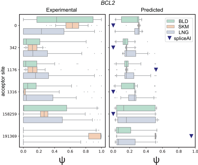
Figure 5. Comparison of the BCL2 gene acceptor sites’ $\psi$, experimental vs predicted. Left: box plots of experimental values (grounds truths) of BCL2 acceptor sites in three different tissues: blood, skeletal muscle and lung, denoted as BLD, SKM and LNG respectively. Right: box plots of predicted $\psi$ for the same group of samples using DCEN; SpliceAI-cls prediction (black triangles) shown for comparison. Please note that SpliceAI-cls prediction uses sequence information only and the prediction will be the same for every sample. Acceptor site coordinates (y-axis) are counted relative to the genomic coordinate of the first exon start of BCL2. Data from 50 samples from each tissue are shown.

6.4.4. Integration of regulatory features allows for sample-specific predictions

An example of a set of model predictions in comparison with the ground truth values for BCL2 gene acceptor sites is shown in Figure 5. Box plots of experimental values (left of Figure 5) represent distributions of $\psi$ in 50 samples for three types of tissues: blood, skeletal muscle and lung. The predictions of DCEN vs SpliceAI-cls for these acceptor sites are shown on the right. We observe that DCEN’s predictions can partially recover the variances in $\psi$ values unique to tissue types (e.g., acceptor site 158259 in Figure 5). When comparing the variance of $\psi$ prediction within each tissue type with the variance of ground-truth $\psi$, the Pearson correlation is 0.177 while the Spearman rank correlation is 0.198. Figure 6 in § A.1 shows the comparison for BCL2 donor sites.

7. Limitations & Future Directions

ARCHS4 database contains data from short-read RNA-seq, and alignment of short reads to quantify transcript isoforms and their respective exons is challenging and an active area of ongoing research (Steijger et al., 2013). Inaccurate attribution of short reads might result in misleading exon counts between transcript isoforms and skewed $\psi$ levels, which limits the prediction usability in a clinical setting.

Another possible issue arises from the fact that samples from the ARCHS4 database are heterogeneous. We speculate that this heterogeneity contributes to the variance in DCEN’s performance across the different tissue types (§ 6.4.3), since the experimental parameters might differ across different labs while collecting the data from these different tissues.

Although we performed batch effect removal with a standard edgeR procedure, batch effects might remain in the data. Homogeneous datasets, as Genotype-Tissue Expression (GTEx) may be used instead, but using ARCHS4 database offers advantages in 1) the diversity of tissue types (healthy and diseased) and 2) its amendable form of data to be further processed for downstream applications.

In the training and evaluation here, the predictions are inferred based on a universal DNA sequence assumed to be the same for all patients. Genomic variations, such as mutations and single nucleotide variants, often lead to aberrant splicing outcomes. One future direction would be to utilize DCEN to study the roles of such genomic variations in the alternative outcomes. Through DCEN’s hierarchical approach of modeling whole transcripts’ probabilities, it is possible to not only draw insights into how mutations can affect inclusion levels of individual splice sites (Jaganathan et al., 2019) but also into the relative expression of transcripts.

8. Conclusions

We curate CAPD to benchmark learning models on alternative splicing (AS) prediction as a regression task, to facilitate future work in this key biological process. By exploiting the compositionality of discrete components, we propose DCEN to predict the AS outcome by modeling mRNA transcripts’ probabilities through its constituent splice junctions’ energy levels. Through our experiments on CAPD, we show that DCEN outperforms baselines and other ablation variants in predicting AS outcomes. Our work shows that deconstructing a task into a hierarchy of discrete components can improve performance in learning models. We hope that DCEN can be used in future work to study RNA regulatory factors’ role in aberrant splicing events.

9. Acknowledgments

This work is supported by the Data Science and Artificial Intelligence Research Center (DSAIR), the School of Computer Science and Engineering at Nanyang Technological University and the Singapore National Research Foundation Investigatorship (NRF-NRFI2017-09).

Appendix A Appendix

A.1. Additional Results

Table 6. Performance of DCEN with early-stopping versus 5x training steps.

Model	Spearman Cor.	Pearson Cor.
Early-Stopped	0.623	0.651
5x Training steps	0.620	0.650

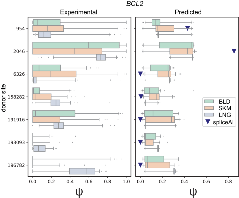
Figure 6. Comparison of the BCL2 gene donor sites’ $\psi$, experimental vs predicted. Left: box plots of experimental values (grounds truths) of BCL2 donor sites in three different tissues: blood, skeletal muscle and lung, denoted as BLD, SKM and LNG respectively. Right: box plots of predicted $\psi$ for the same group of samples using DCEN; SpliceAI-cls prediction (black triangles) shown for comparison. Please note that SpliceAI-cls prediction uses sequence information only and the prediction will be the same for every sample. Donor site coordinates (y axis) are counted relative to the genomic coordinate of the first exon start of BCL2. Data from 50 samples from each tissue are shown.

A.2. Proof

Theorem A.1.

Given the energy levels of all the possible discrete states of a system, the probability of a particular state $T_{i}$ is the softmax output of its energy $E_{T_{i}}$ with respect to those of all other possible states in the system, i.e.,

(9) $$P_{i}=\frac{\exp(-E_{T_{i}})}{\sum_{j}\exp(-E_{T_{j}})}=\mathrm{Softmax}_{i}(E)$$

Proof.

From Boltzmann distribution, the probability that a system takes on a particular state ($x$) can be expressed as:

(10) $$p_{\theta}(x) =\frac{\exp{(-E_{\theta}(x)})}{Z(\theta)}$$

$$=\frac{h(x)}{Z(\theta)}$$

where

(11) $$Z(\theta) =\int\exp{(-E_{\theta}(x))}~{}dx$$

$$=\int h(x)~{}dx$$

is known as the partition function.

Since the probabilities of all possible states sum to 1, we have

(12) $$1=\operatorname{\mathbb{E}}_{x\sim p_{\theta}}[1]=\sum_{x}\frac{h(x)}{Z}$$

which gives

(13) $$Z=\sum_{x}h(x)~{}.$$

Through importance sampling with another probability distribution $q$, we can express $Z$ as

(14) $$Z =\sum_{x}\frac{h(x)}{q(x)}q(x)$$

$$=\frac{1}{n}\sum_{i}\frac{h(x_{i})}{q(x_{i})}~{}~{}~{},~{}~{}~{}~{}~{}x_{i}\sim q~{}.$$

Using an uniform discrete distribution as $q$ where all $k$ possible states ($x_{i}$) have the same probability $q(x_{i})=(1/k)$, we get

(15) $$Z =\frac{1}{k}\sum_{i}\frac{h(x_{i})}{(1/k)}$$

$$=\sum_{i}h(x_{i})$$

Combining Eq. (11) and (15), this gives

(16) $$p_{\theta}(x_{i}) =\frac{h(x_{i})}{\sum_{j}h(x_{j})}$$

$$=\frac{\exp{(-E_{\theta}(x_{i})})}{\sum_{j}\exp{(-E_{\theta}(x_{j})})}$$

$$=\mathrm{Softmax}_{i}(E)$$

∎

References

- (1)
- Barash et al. (2010) Yoseph Barash, John A. Calarco, Weijun Gao, Qun Pan, Xinchen Wang, Ofer Shai, Benjamin J. Blencowe, and Brendan J. Frey. 2010. Deciphering the splicing code. Nature (2010). https://doi.org/10.1038/nature09000
- Basturea (2013) Georgeta N. Basturea. 2013. Research Methods for Detection and Quantitation of RNA Modifications. Materials and Methods (2013). https://doi.org/10.13070/mm.en.3.186
- Boo and Kim (2020) Sung Ho Boo and Yoon Ki Kim. 2020. The emerging role of RNA modifications in the regulation of mRNA stability. https://doi.org/10.1038/s12276-020-0407-z
- Bretschneider et al. (2018) Hannes Bretschneider, Shreshth Gandhi, Amit G. Deshwar, Khalid Zuberi, and Brendan J. Frey. 2018. COSSMO: Predicting competitive alternative splice site selection using deep learning. In Bioinformatics. https://doi.org/10.1093/bioinformatics/bty244
- Bryant et al. (2012) Douglas W. Bryant, Henry D. Priest, and Todd C. Mockler. 2012. Detection and quantification of alternative splicing variants using RNA-seq. Methods in Molecular Biology (2012). https://doi.org/10.1007/978-1-61779-839-9_7
- Cheng et al. (2020) Jun Cheng, Muhammed Hasan Celik, Anshul Kundaje, and Julien Gagneur. 2020. MTSplice predicts effects of genetic variants on tissue-specific splicing. bioRxiv (2020).
- Cheng et al. (2019) Jun Cheng, Thi Yen Duong Nguyen, Kamil J Cygan, Muhammed Hasan Çelik, William G Fairbrother, Julien Gagneur, et al. 2019. MMSplice: modular modeling improves the predictions of genetic variant effects on splicing. Genome biology 20, 1 (2019), 1–15.
- Cook et al. (2011) Kate B. Cook, Hilal Kazan, Khalid Zuberi, Quaid Morris, and Timothy R. Hughes. 2011. RBPDB: A database of RNA-binding specificities. Nucleic Acids Research (2011). https://doi.org/10.1093/nar/gkq1069
- Degroeve et al. (2005) Sven Degroeve, Yvan Saeys, Bernard De Baets, Pierre Rouzé, and Yves Van de Peer. 2005. SpliceMachine: Predicting splice sites from high-dimensional local context representations. Bioinformatics (2005). https://doi.org/10.1093/bioinformatics/bti166
- Du et al. (2019) Yilun Du, Shuang Li, and Igor Mordatch. 2019. Compositional Visual Generation with Energy Based Models. (2019).
- Du et al. (2020) Yilun Du, Joshua Meier, Jerry Ma, Rob Fergus, and Alexander Rives. 2020. Energy-based models for atomic-resolution protein conformations. arXiv preprint arXiv:2004.13167 (2020).
- Du and Mordatch (2019) Yilun Du and Igor Mordatch. 2019. Implicit generation and generalization in energy-based models. arXiv preprint arXiv:1903.08689 (2019).
- Frankish et al. (2019) Adam Frankish, Mark Diekhans, Anne Maud Ferreira, Rory Johnson, Irwin Jungreis, Jane Loveland, Jonathan M. Mudge, Cristina Sisu, James Wright, Joel Armstrong, If Barnes, Andrew Berry, Alexandra Bignell, Silvia Carbonell Sala, Jacqueline Chrast, Fiona Cunningham, Tomás Di Domenico, Sarah Donaldson, Ian T. Fiddes, Carlos García Girón, Jose Manuel Gonzalez, Tiago Grego, Matthew Hardy, Thibaut Hourlier, Toby Hunt, Osagie G. Izuogu, Julien Lagarde, Fergal J. Martin, Laura Martínez, Shamika Mohanan, Paul Muir, Fabio C.P. Navarro, Anne Parker, Baikang Pei, Fernando Pozo, Magali Ruffier, Bianca M. Schmitt, Eloise Stapleton, Marie Marthe Suner, Irina Sycheva, Barbara Uszczynska-Ratajczak, Jinuri Xu, Andrew Yates, Daniel Zerbino, Yan Zhang, Bronwen Aken, Jyoti S. Choudhary, Mark Gerstein, Roderic Guigó, Tim J.P. Hubbard, Manolis Kellis, Benedict Paten, Alexandre Reymond, Michael L. Tress, and Paul Flicek. 2019. GENCODE reference annotation for the human and mouse genomes. Nucleic Acids Research (2019). https://doi.org/10.1093/nar/gky955
- Gallego-Paez et al. (2017) L. M. Gallego-Paez, M. C. Bordone, A. C. Leote, N. Saraiva-Agostinho, M. Ascensão-Ferreira, and N. L. Barbosa-Morais. 2017. Alternative splicing: the pledge, the turn, and the prestige: The key role of alternative splicing in human biological systems. https://doi.org/10.1007/s00439-017-1790-y
- Grathwohl et al. (2019) Will Grathwohl, Kuan-Chieh Wang, Jörn-Henrik Jacobsen, David Duvenaud, Mohammad Norouzi, and Kevin Swersky. 2019. Your classifier is secretly an energy based model and you should treat it like one. arXiv preprint arXiv:1912.03263 (2019).
- Haarnoja et al. (2017) Tuomas Haarnoja, Haoran Tang, Pieter Abbeel, and Sergey Levine. 2017. Reinforcement learning with deep energy-based policies. arXiv preprint arXiv:1702.08165 (2017).
- He et al. (2016) Kaiming He, Xiangyu Zhang, Shaoqing Ren, and Jian Sun. 2016. Deep residual learning for image recognition. In Proceedings of the IEEE conference on computer vision and pattern recognition. 770–778.
- Huang and Sanguinetti (2017) Yuanhua Huang and Guido Sanguinetti. 2017. BRIE: Transcriptome-wide splicing quantification in single cells. Genome Biology (2017). https://doi.org/10.1186/s13059-017-1248-5
- Jaganathan et al. (2019) Kishore Jaganathan, Sofia Kyriazopoulou Panagiotopoulou, Jeremy F. McRae, Siavash Fazel Darbandi, David Knowles, Yang I. Li, Jack A. Kosmicki, Juan Arbelaez, Wenwu Cui, Grace B. Schwartz, Eric D. Chow, Efstathios Kanterakis, Hong Gao, Amirali Kia, Serafim Batzoglou, Stephan J. Sanders, and Kyle Kai How Farh. 2019. Predicting Splicing from Primary Sequence with Deep Learning. Cell (2019). https://doi.org/10.1016/j.cell.2018.12.015
- Jha et al. (2017) Anupama Jha, Matthew R Gazzara, and Yoseph Barash. 2017. Integrative deep models for alternative splicing. Bioinformatics 33, 14 (2017), i274–i282.
- Lachmann et al. (2018) Alexander Lachmann, Denis Torre, Alexandra B. Keenan, Kathleen M. Jagodnik, Hoyjin J. Lee, Lily Wang, Moshe C. Silverstein, and Avi Ma’ayan. 2018. Massive mining of publicly available RNA-seq data from human and mouse. Nature Communications (2018). https://doi.org/10.1038/s41467-018-03751-6
- LeCun et al. (2006) Yann LeCun, Sumit Chopra, Raia Hadsell, M Ranzato, and F Huang. 2006. A tutorial on energy-based learning. Predicting structured data 1, 0 (2006).
- Leung et al. (2014) Michael K.K. Leung, Hui Yuan Xiong, Leo J. Lee, and Brendan J. Frey. 2014. Deep learning of the tissue-regulated splicing code. Bioinformatics (2014). https://doi.org/10.1093/bioinformatics/btu277
- Louadi et al. (2019) Zakaria Louadi, Mhaned Oubounyt, Hilal Tayara, and Kil To Chong. 2019. Deep splicing code: Classifying alternative splicing events using deep learning. Genes (2019). https://doi.org/10.3390/genes10080587
- Mortazavi et al. (2008) Ali Mortazavi, Brian A. Williams, Kenneth McCue, Lorian Schaeffer, and Barbara Wold. 2008. Mapping and quantifying mammalian transcriptomes by RNA-Seq. Nature Methods (2008). https://doi.org/10.1038/nmeth.1226
- Nijkamp et al. (2019) Erik Nijkamp, Mitch Hill, Song-Chun Zhu, and Ying Nian Wu. 2019. Learning non-convergent non-persistent short-run MCMC toward energy-based model. In Advances in Neural Information Processing Systems. 5232–5242.
- Oldham et al. (2008) Michael C. Oldham, Genevieve Konopka, Kazuya Iwamoto, Peter Langfelder, Tadafumi Kato, Steve Horvath, and Daniel H. Geschwind. 2008. Functional organization of the transcriptome in human brain. Nature Neuroscience (2008). https://doi.org/10.1038/nn.2207
- Pertea et al. (2001) M. Pertea, X. Lin, and S. L. Salzberg. 2001. GeneSplicer: A new computational method for splice site prediction. Nucleic Acids Research (2001). https://doi.org/10.1093/nar/29.5.1185
- Robinson et al. (2009) Mark D. Robinson, Davis J. McCarthy, and Gordon K. Smyth. 2009. edgeR: A Bioconductor package for differential expression analysis of digital gene expression data. Bioinformatics (2009). https://doi.org/10.1093/bioinformatics/btp616
- Sibley et al. (2015) Christopher R. Sibley, Warren Emmett, Lorea Blazquez, Ana Faro, Nejc Haberman, Michael Briese, Daniah Trabzuni, Mina Ryten, Michael E. Weale, John Hardy, Miha Modic, Tomaž Curk, Stephen W. Wilson, Vincent Plagnol, and Jernej Ule. 2015. Recursive splicing in long vertebrate genes. Nature (2015). https://doi.org/10.1038/nature14466
- Song and Ou (2018) Yunfu Song and Zhijian Ou. 2018. Learning neural random fields with inclusive auxiliary generators. arXiv preprint arXiv:1806.00271 (2018).
- Steijger et al. (2013) Tamara Steijger, Josep F. Abril, Pär G. Engström, Felix Kokocinski, Martin Akerman, Tyler Alioto, Giovanna Ambrosini, Stylianos E. Antonarakis, Jonas Behr, Paul Bertone, Regina Bohnert, Philipp Bucher, Nicole Cloonan, Thomas Derrien, Sarah Djebali, Jiang Du, Sandrine Dudoit, Mark Gerstein, Thomas R. Gingeras, David Gonzalez, Sean M. Grimmond, Roderic Guigó, Lukas Habegger, Jennifer Harrow, Tim J. Hubbard, Christian Iseli, Géraldine Jean, André Kahles, Julien Lagarde, Jing Leng, Gregory Lefebvre, Suzanna Lewis, Ali Mortazavi, Peter Niermann, Gunnar Rätsch, Alexandre Reymond, Paolo Ribeca, Hugues Richard, Jacques Rougemont, Joel Rozowsky, Michael Sammeth, Andrea Sboner, Marcel H. Schulz, Steven M.J. Searle, Naryttza Diaz Solorzano, Victor Solovyev, Mario Stanke, Brian J. Stevenson, Heinz Stockinger, Armand Valsesia, David Weese, Simon White, Barbara J. Wold, Jie Wu, Thomas D. Wu, Georg Zeller, Daniel Zerbino, and Michael Q. Zhang. 2013. Assessment of transcript reconstruction methods for RNA-seq. Nature Methods (2013). https://doi.org/10.1038/nmeth.2714
- Suzuki et al. (2013) Hitoshi Suzuki, Toshiki Kameyama, Kenji Ohe, Toshifumi Tsukahara, and Akila Mayeda. 2013. Nested introns in an intron: Evidence of multi-step splicing in a large intron of the human dystrophin pre-mRNA. FEBS Letters (2013). https://doi.org/10.1016/j.febslet.2013.01.057
- Taladriz-Sender et al. (2019) Andrea Taladriz-Sender, Emma Campbell, and Glenn A. Burley. 2019. Splice-switching small molecules: A new therapeutic approach to modulate gene expression. Methods (2019). https://doi.org/10.1016/j.ymeth.2019.06.011
- Tazi et al. (2009) Jamal Tazi, Nadia Bakkour, and Stefan Stamm. 2009. Alternative splicing and disease. https://doi.org/10.1016/j.bbadis.2008.09.017
- Wang et al. (2008) Eric T. Wang, Rickard Sandberg, Shujun Luo, Irina Khrebtukova, Lu Zhang, Christine Mayr, Stephen F. Kingsmore, Gary P. Schroth, and Christopher B. Burge. 2008. Alternative isoform regulation in human tissue transcriptomes. Nature (2008). https://doi.org/10.1038/nature07509
- Witten and Ule (2011) Joshua T. Witten and Jernej Ule. 2011. Understanding splicing regulation through RNA splicing maps. https://doi.org/10.1016/j.tig.2010.12.001
- Xie et al. (2016) Jianwen Xie, Yang Lu, Song-Chun Zhu, and Yingnian Wu. 2016. A theory of generative convnet. In International Conference on Machine Learning. 2635–2644.
- Xiong et al. (2015) Hui Y. Xiong, Babak Alipanahi, Leo J. Lee, Hannes Bretschneider, Daniele Merico, Ryan K.C. Yuen, Yimin Hua, Serge Gueroussov, Hamed S. Najafabadi, Timothy R. Hughes, Quaid Morris, Yoseph Barash, Adrian R. Krainer, Nebojsa Jojic, Stephen W. Scherer, Benjamin J. Blencowe, and Brendan J. Frey. 2015. The human splicing code reveals new insights into the genetic determinants of disease. Science (2015). https://doi.org/10.1126/science.1254806
- Xiong et al. (2011) Hui Yuan Xiong, Yoseph Barash, and Brendan J. Frey. 2011. Bayesian prediction of tissue-regulated splicing using RNA sequence and cellular context. Bioinformatics (2011). https://doi.org/10.1093/bioinformatics/btr444
- Yee et al. (2019) Brian A. Yee, Gabriel A. Pratt, Brenton R. Graveley, Eric L. van Nostrand, and Gene W. Yeo. 2019. RBP-Maps enables robust generation of splicing regulatory maps. RNA (2019). https://doi.org/10.1261/rna.069237.118
- Zerbino (2018) Daniel R. et al. Zerbino. 2018. Ensembl 2018. Nucleic Acids Research (2018). https://doi.org/10.1093/nar/gkx1098
- Zhang et al. (2018) Yi Zhang, Xinan Liu, James MacLeod, and Jinze Liu. 2018. Discerning novel splice junctions derived from RNA-seq alignment: A deep learning approach. BMC Genomics (2018). https://doi.org/10.1186/s12864-018-5350-1
- Zhang et al. (2019) Zijun Zhang, Zhicheng Pan, Yi Ying, Zhijie Xie, Samir Adhikari, John Phillips, Russ P. Carstens, Douglas L. Black, Yingnian Wu, and Yi Xing. 2019. Deep-learning augmented RNA-seq analysis of transcript splicing. Nature Methods (2019). https://doi.org/10.1038/s41592-019-0351-9
- Zuallaert et al. (2018) Jasper Zuallaert, Fréderic Godin, Mijung Kim, Arne Soete, Yvan Saeys, and Wesley De Neve. 2018. Splicerover: Interpretable convolutional neural networks for improved splice site prediction. Bioinformatics (2018). https://doi.org/10.1093/bioinformatics/bty497