Inverse Kohn-Sham Density Functional Theory: Progress and Challenges

Abstract

Inverse Kohn-Sham (iKS) problems are needed to fully understand the one-to-one mapping between densities and potentials on which Density Functional Theory is based. They are also important to advance computational schemes that rely on density-to-potential inversions such as the Optimized Effective Potential method and various techniques for density-based embedding. Unlike the forward Kohn-Sham problems, numerical iKS problems are ill-posed and can be unstable. We discuss some of the fundamental and practical difficulties of iKS problems with constrained-optimization methods on finite basis sets. Various factors that affect the performance are systematically compared and discussed, both analytically and numerically, with a focus on two of the most practical methods: the Wu-Yang method (WY) and partial-differential-equation constrained-optimization (PDE-CO). Our analysis of the WY and PDE-CO highlights the limitation of finite basis sets and the importance of regularization. We introduce two new ideas that will hopefully contribute to making iKS problems more tractable: (1) A correction to the WY method that utilizes the null space of the relevant Hessian matrices; and (2) A finite potential basis-set implementation of the PDE-CO method. We provide an overall strategy for performing numerical density-to-potential inversions that can be directly adopted in practice. We also provide an Appendix with several examples that can be used for benchmarking.

I Introduction

In principle vs. in practice: Kohn-Sham (KS) density functional theory (DFT) Hohenberg and Kohn (1964); Kohn and Sham (1965) has long been the most widely used method for electronic-structure calculations in condensed matter physics and quantum chemistry computations Burke (2012); Verma and Truhlar (2020). KS-DFT is formally exact in the sense that, given the exact exchange-correlation (XC) energy functional, a numerically exact solution of the self-consistent KS-DFT equations is guaranteed to yield the exact ground-state density $n({\bf r})$ and energy for any system of $N$ electrons in a time-independent external potential $v({\bf r})$. The word ”exact”, which has been used 4 times already in this introductory paragraph, is sometimes dismissed with scorn when confronted with results in practice. The results of actual DFT calculations are evidently not exact. Nevertheless, it is the proven existence of an exact one-to-one correspondence between ground-state densities and potentials which has given impetus to the development of approximations in DFT. A different one-to-one mapping exists for any choice of electron-electron interaction. Nature’s choice is the Coulomb interaction, but the correspondence can be established also for a fictitious system of non-interacting electrons. Calculations are simpler in this fictitious world, and the one-to-one maps allow one to connect the answers back to the real world, in principle. In practice, the exchange-correlation energy $E_{\scriptscriptstyle\rm XC}[n]$, “nature’s glue” Kurth and Perdew (2000), needs to be approximated. This paper discusses another clash between “in-principle” and “in practice”: The density-to-potential mappings are in principle one-to-one. For a given density $n({\bf r})$ and choice of approximate $E_{\scriptscriptstyle\rm XC}[n]$, there is in principle only one XC potential $v_{\scriptscriptstyle\rm XC}({\bf r})$ corresponding to $n({\bf r})$. That potential is the functional derivative of $E_{\scriptscriptstyle\rm XC}[n]$ with respect to the density, evaluated at that density. The potential $v_{\scriptscriptstyle\rm XC}({\bf r})$ should be calculable from the given density by solving an inverse problem, in principle. In practice, unfortunately, the process is a numerical minefield. For a user’s choice of approximate $E_{\scriptscriptstyle\rm XC}[n]$, most quantum-chemistry codes solve the forward KS-DFT problem, i.e. self-consistently calculate $n({\bf r})$ and, from it, the total energy for a given $v({\bf r})$ and $N$. Another output of this calculation is the self-consistent $v_{\scriptscriptstyle\rm XC}({\bf r})$. Much less common are codes that can solve the inverse Kohn-Sham problem (iKS) to find the XC potential corresponding to a given densityNam et al. (2020a); Unsleber et al. (2018). But why would one want to do such calculations? We list four answers below:

• Exploring the Hohenberg-Kohn Hohenberg and Kohn (1964) and Runge-Gross Runge and Gross (1984) mappings: More generally, density-to-potential inversions are useful for calculating numerically exact XC potentials from numerically exact densities, i.e. a point-by-point exploration of the Hohenberg-Kohn and Runge-Gross mappings. In ground-state DFT, inversions can reveal features of XC potentials that encode the physics of strong correlations Helbig, Tokatly, and Rubio (2009); Hodgson et al. (2017) and are missed by approximate functionals. In time-dependent DFT, inversions can also shed light on properties of the exact time-dependent XC potentials needed to describe electronic dynamics Thiele and Kummel (2009); Fuks et al. (2016), and to propose approximations that go beyond the adiabatic limit Maitra et al. (2004); Maitra (2016); ramsden2012exact; mancini2014adiabatic, as needed for describing multiple and charge-transfer excitations in molecules or excitonic transitions in solids.

• Analyzing errors of approximate XC functionals: iKS can be utilized for measuring density-driven errors in KS-DFT Nam et al. (2020b); iKS from numerically exact densities can assist on the development of explicit XC functionals. There are also recent examples of the use of iKS to improve XC functionals in the field of nuclear DFT Naito, Ohashi, and Liang (2019); Accorto et al. (2020, 2021). Furthermore, machine-learning approaches under development Brockherde et al. (2017); Nagai et al. (2018); Kalita et al. (2021); Manzhos (2020) also take inverted XC potentials as input. The efficiency and accuracy of the iKS methods is critically important here.

• Quantum Embedding: Various modern variants of density-based subsystem and embedding approaches Jacob and Neugebauer (2014); Wesolowski, Shedge, and Zhou (2015) employ potential reconstruction techniques Goodpaster et al. (2010); Nafziger, Wu, and Wasserman (2011); Huang, Pavone, and Carter (2011). Here, typically, a target density is updated many times in a self-consistent loop and the potential corresponding to that target density must be found at each step of the loop, implying a significant additional computational cost to calculations that do not make use of efficient inversion techniques.

• Optimized Effective Potentials (OEP): Approximate expressions for $E_{\scriptscriptstyle\rm XC}[n]$ can be either explicit or implicit functionals of the density. Explicit functionals are usually preferred for their simplicity and efficiency. However, implicit XC functionals Kummel and Kronik (2008) that depend on the KS orbitals are often used when higher accuracy is needed Levy (1979); Perdew et al. (2005). In particular, OEP methods are being increasingly used for a variety of applications Jin et al. (2017a, b); Flick et al. (2018). The OEP method is often the bottleneck of the calculations. The direct OEP method developed by Yang and WuYang and Wu (2002) shares many of the same features of iKS discussed here Gidopoulos and Lathiotakis (2012); Bulat et al. (2007); Heaton-Burgess and Yang (2008). Improvements on inversion methods would potentially offer significant speed-ups allowing for more widespread adoption of OEP calculations.

iKS methods: Several methods exist for solving the iKS problem through self-consistent density-based calculations Aryasetiawan and Stott (1988); Görling (1992); Zhao and Parr (1992, 1993); Wang and Parr (1993); Peirs, Van Neck, and Waroquier (2003); Kadantsev and Stott (2004); Wagner et al. (2014); Ou and Carter (2018). The connections between many of these methods have been cogently explored recently by Kumar et al.Kumar, Singh, and Harbola (2019); Kumar and Harbola (2020). An entirely different approach that makes use of the wavefunction (instead of the density) has been developed by Ryabinkin, Kohut, and Staroverov (mRKS) and shown to provide arguably the best inversion results to date Ryabinkin, Kohut, and Staroverov (2015); Ospadov, Ryabinkin, and Staroverov (2017). mRKS uses as input the one- and two-particle reduced density matrices. Its computational cost is thus out of reach for calculations on large systems. A detailed discussion explaining the success of wavefunction based methods compared to pure density inversions was provided recently by Kumar et al.Kumar, Singh, and Harbola (2020). We concentrate on pure Kohn-Sham inversions, referred to as iKS in this Perspective. We use mRKS in this article as benchmark to compare with other purely density-based approaches. Methods other than self-consistent calculations have also been designed, many of which feature constrained optimizations Zhao, Morrison, and Parr (1994); Wu, Ayers, and Yang (2003); Nafziger, Jiang, and Wasserman (2017); Jensen and Wasserman (2018); Kanungo, Zimmerman, and Gavini (2019); Kumar and Harbola (2020); Callow, Lathiotakis, and Gidopoulos (2020).

In spite of all the methods in hand, iKS problems are still difficult. First, different methods feature different capabilities regarding accuracy and efficiency. Many of them have been only tested on single atoms or diatomic molecules for illustration. Some accurate methods, such as mRKS, are difficult to apply to molecules with more than $\sim$10 atoms. Kanungo, Zimmerman, and Gavini recently implemented the PDE-Constrained Optimization method (PDE-CO) on a systematically improvable finite-element basis that provided results for polyatomic systems with an accuracy comparable to that of mRKS using affordable computation resources Kanungo, Zimmerman, and Gavini (2019). KS inversions on finite basis sets are generally considered as ill-posed. A problem is well-posed if a solution exists, it is unique and continuously changes with the input as defined by Hadamard Hadamard (1902). If a problem is not well-posed, it is then ill-posed. Analogous inverse problems in many fields are generally known for their instabilities. In the case of iKS, the uniqueness is guaranteed by the Hohenberg-Kohn theorem. The existence is known as the $v$-representability problem. In discretized systems, densities are ensemble $v$-representable Chayes, Chayes, and Ruskai (1985); Ullrich and Kohn (2002); Lammert (2006). The existence is usually assumed to be true. The main problem of KS inversion lays in the continuity of the density-to-potential mapping Jensen and Wasserman (2018). Since the kinetic operator in the KS equation plays a role of regulator, different XC potentials can reproduce very similar densities Nagai et al. (2018); Li et al. (2020); Nagai, Akashi, and Sugino (2020). In practical KS inversion calculations on finite basis sets, many factors can lead to unphysical oscillations/overfitting to the final $v_{\scriptscriptstyle\rm XC}({\bf r})$. Therefore, special consideration and regularization is often essential for reasonable results. Simple tricks can often greatly improve an inversion when using one particular inversion method but those same tricks may be totally unhelpful when used in combination with other methods. Many of these tricks depend on error cancellations of some form Gaiduk, Ryabinkin, and Staroverov (2013); Kanungo, Zimmerman, and Gavini (2019); Wu and Yang (2003); Ospadov, Ryabinkin, and Staroverov (2017); Bulat et al. (2007); Heaton-Burgess and Yang (2008); Jacob (2011); Nam et al. (2020a), making it extremely difficult to predict when they will work or fail.

Organization of this paper: We focus on two of the most efficient constrained-optimization methods for iKS, the Wu-Yang method Wu and Yang (2003) (WY) and PDE-Constrained Optimization Nafziger, Jiang, and Wasserman (2017); Jensen and Wasserman (2018) (PDE-CO). First, we review the theory behind both methods and their implementation on finite basis sets, including the first implementation of PDE-CO on Gaussian potential basis sets. Except for the well-known drawbacks of the finite potential basis set (PBS), PBS significantly improves the efficiency and helps to control problems that one would encounter in a general PDE-CO problem Jensen and Wasserman (2018); Kanungo, Zimmerman, and Gavini (2019); Vogel (2002). Different factors that influence the stability of the inversion are systemically discussed and compared, both analytically and numerically, including finite basis sets, regularization/corrections, optimization methods and guide potentials. There is no way of avoiding the use of many different acronyms for the methods, algorithms, and basis sets employed here. Table 1 compiles the acronyms we use most. We highlight our use of “CX/CY” when cc-pCVXZ is being used as the basis set to expand the orbitals and cc-pCVYZ as the basis set to expand the potentials. The input density is CCSD unless further specified. The exact XC potential data comes from quantum Monte Carlo calculations Umrigar and Gonze (1994); Filippi, Gonze, and Umrigar (1996). All the calculations are implemented on Psi4 Parrish et al. (2017); Smith et al. (2018). Atomic units are used throughout.

CCSD	coupled-cluster singles-
	and-doubles
CX	cc-pCVXZ
CX/CY	The OBS/PBS is CX/CY
FA	Fermi-Amaldi
iKS	inverse Kohn-Sham
KS	Kohn-Sham
LDA	Local Density Approximation
mRKS	modified Ryabinkin–
	Kohut–Staroverov
NSC	null-space correction
OBS	atomic orbital basis set
NSC	null space correction
PBS	potential basis set
PBE	Perdew-Burke-Ernzerhof
PDE	partial differential equation
PDE-CO	PDE-Constrained optimization
QMC	quantum Monte Carlo
TSVD	truncated singular value
	decomposition
WY	the Wu-Yang method
XC	exchange-correlation

Table 1: Acronym List

II Theory

II.1 The Wu-Yang Method (WY)

The central idea of the WY method follows directly the Levy constrained-search approach for the KS kinetic energy functional Levy (1979); Kohn and Sham (1965): optimizing the non-interacting kinetic energy under the constraint that the density matches a target. Unlike many other methods that depend on some sort of self-consistent calculation, the WY method relies on gradient and Hessian-based optimizations. Thus the WY method can be very easily implemented with a standard general optimizer and is robust for most systems. On the other hand, given the ill-posed nature of iKS and the ill-conditioning of the Hessian matrices, there can be numerical problems and regularization is usually essential.

The Lagrangian for the WY constrained optimization is

$$\begin{split}&W[\Psi_{\rm det}[v_{\scriptscriptstyle\rm KS}],v_{\scriptscriptstyle\rm KS}]\\ =&T_{s}[\Psi_{\rm det}]+\int d{\bf r}v_{\scriptscriptstyle\rm KS}({\bf r})\{n({\bf r})-n_{\rm in}({\bf r})\},\end{split}$$ (1)

where $n_{\rm in}({\bf r})$ is the target input density and $n({\bf r})$ is:

$$n({\bf r}) =N\int d{\bf r}_{2}\dots d{\bf r}_{N}|\Psi_{\rm det}({\bf r},{\bf r}_{2},\dots,{\bf r}_{N})|^{2}$$ (2a)

$$=2\sum_{i}^{N/2}|\psi_{i}({\bf r})|^{2}.$$ (2b)

The $\Psi_{\rm det}$ in Eqs.(1)-(2) is the KS Slater determinant consisting of $N/2$ doubly occupied orthonormal KS orbitals $\{\psi_{i}\}$. Our discussions will be limited to spin-unpolarized systems for convenience. $v_{\scriptscriptstyle\rm KS}({\bf r})$ in Eq.(1) is the KS potential:

$$[\hat{T}+v_{\scriptscriptstyle\rm KS}({\bf r})]\psi_{i}({\bf r})=\epsilon_{i}\psi_{i}({\bf r})~{}~{},$$ (3)

but appears in Eq.(1) as a Lagrange multiplier because of the necessary condition on the stationary point:

$$\frac{\delta W[\Psi_{\rm det},v_{\scriptscriptstyle\rm KS}]}{\delta n({\bf r})}=0.$$ (4)

Here, a Lagrangian dual problem of the Zhao-Morrison-Parr Zhao, Morrison, and Parr (1994) problem is solved and $v_{\scriptscriptstyle\rm XC}({\bf r})$ is the dual variable of the density Wu (2014); Kumar and Harbola (2020). Therefore, (1) needs to be maximized. This will also be proven later through features of the hessian matrices.

From (1):

$$\frac{\delta W[\Psi_{\rm det}[v_{\scriptscriptstyle\rm KS}],v_{\scriptscriptstyle\rm KS}]}{\delta v_{\scriptscriptstyle\rm KS}({\bf r})}=n({\bf r})-n_{\rm in}({\bf r})$$ (5)

and

$$\begin{split}&\frac{\delta^{2}W[\Psi_{\rm det}[v_{\rm KS}],v_{\rm KS}]}{\delta v_{\scriptscriptstyle\rm KS}({\bf r})\delta v_{\scriptscriptstyle\rm KS}({\bf r}^{\prime})}=\frac{\delta n({\bf r})}{\delta v_{KS}({\bf r}^{\prime})}\\ =&2\sum_{i}^{occ.}\sum_{a}^{unocc.}\frac{\psi_{i}^{*}({\bf r})\psi_{a}({\bf r})\psi_{i}({\bf r}^{\prime})\psi_{a}^{*}({\bf r}^{\prime})}{\epsilon_{i}-\epsilon_{a}}.\end{split}$$ (6)

II.2 PDE-Constrained Optimization (PDE-CO)

Based on the Hohenberg-Kohn theorem Hohenberg and Kohn (1964) and assuming non-degeneracy, one would expect from an “exact” input density the exact KS potential. The continuity condition in the definition of well-posed problems is not proven, but it is generally assumed to hold (at least around the ”exact” density): a more accurate potential is expected to yield a more accurate density and vice versa. To find the best $v_{\scriptscriptstyle\rm KS}({\bf r})$ given the limitation of a basis set or a grid, searching for a density that is closest to the “exact” input density is usually a good idea. To do this, one could define a density error function to minimize:

$${\rm arg~{}min}_{v_{\scriptscriptstyle\rm KS}({\bf r})}\int d{\bf r}u({\bf r})|n({\bf r})-n_{\rm in}({\bf r})|^{w}.$$ (7)

subject to constraints (3) and:

$$\int|\psi_{i}({\bf r})|^{2}d{\bf r}=1.$$ (8)

$u({\bf r})$ in (7) can be a positive weight function that should not change the final convergence theoretically. $u({\bf r})=\frac{1}{n({\bf r})^{p}}$ for $p\in[1,2)$ can be helpful for the asymptotic region when $v_{\scriptscriptstyle\rm KS}({\bf r})$ is calculated on a grid. Properties of the weight function $u({\bf r})$ when calculations are performed on a grid can be found in the recent work by Kanungo et al.Kanungo, Zimmerman, and Gavini (2019). Because in our basis-set implementation $v_{\scriptscriptstyle\rm KS}({\bf r})$ is expanded as in (11), the asymptotic behavior is determined by $v_{0}({\bf r})$ (see below) and we use $u({\bf r})=1$ and $w=2$ in what follows. Note that Eq.(7) is just the simplest form of an error function. The main reason to choose this form is to derive the gradient analytically, as we will do. However, with the help of automatic differentiationBaydin et al. (2018), more sophisticated error functions can be designed.

The Lagrangian can be written as

$$\begin{split}&L[v_{\scriptscriptstyle\rm KS},\{\psi_{i}\},\{\epsilon_{i}\},\{p_{i}\},\{\mu_{i}\}]\\ =&\int(n({\bf r})-n_{\rm in}({\bf r}))^{2}d{\bf r}\\ &+\sum_{i=1}^{N/2}\int p_{i}({\bf r})(-\frac{1}{2}\nabla^{2}+v_{\scriptscriptstyle\rm KS}-\epsilon_{i})\psi_{i}d{\bf r}\\ &+\sum_{i=1}^{N/2}\mu_{i}(\int|\psi_{i}({\bf r})|^{2}d{\bf r}-1),\end{split}$$ (9)

where $p_{i}({\bf r})$ and $\mu_{i}$ are the Lagrange multipliers introduced for (3) and (8). Variations with respect to the $\psi_{i}({\bf r})$, $\epsilon_{i}$ and $v_{\scriptscriptstyle\rm KS}({\bf r})$ yield:

$$\begin{split}&(-\frac{1}{2}\nabla^{2}+v_{\scriptscriptstyle\rm KS}({\bf r})-\epsilon_{i})p_{i}({\bf r})=8\times\\ &~{}~{}~{}(n_{\rm in}({\bf r})-n({\bf r}))\psi_{i}({\bf r})-2\mu_{i}\psi_{i}({\bf r}),\end{split}$$ (10a)

$$\int p_{i}({\bf r})\psi_{i}({\bf r})d{\bf r}=0,$$ (10b)

$$\frac{\delta L}{\delta v_{\scriptscriptstyle\rm KS}({\bf r})}=\sum_{i=1}^{N/2}p_{i}({\bf r})\psi_{i}({\bf r}).$$ (10c)

The optimization strategy generally adopted is to solve for the $p_{i}({\bf r})$ and the $\psi_{i}({\bf r})$ from (3), (10a) and (10b) and build $\frac{\delta L}{\delta v_{KS}}$ from (10c) for each step. The shape of $L[v_{KS},\{\psi_{i}\},\{\epsilon_{i}\},\{p_{i}\},\{\mu_{i}\}]$ can be arbitrary (not necessarily convex or concave). Thus, a good initial guess for $v_{\scriptscriptstyle\rm KS}({\bf r})$ is important to find the stationary point of the Lagrangian.

III Potential Basis Sets (PBS)

There is a general trade-off between the accuracy and efficiency in iKS. Using a PBS improves the efficiency significantly. The original WY method Wu and Yang (2003) represented $v_{\scriptscriptstyle\rm KS}({\bf r})$ as:

$$v_{\scriptscriptstyle\rm KS}({\bf r})=v_{\rm ext}({\bf r})+v_{0}({\bf r})+v_{\rm PBS}({\bf r})$$ (11)

where $v_{\rm ext}({\bf r})$ is the external potential due to the nuclei and $v_{0}({\bf r})$ is a guide potential, whose role is discussed below. The rest is expanded on a finite potential basis set (PBS) $\{\phi_{t}\}$

$$v_{\rm PBS}({\bf r})=\sum_{t}b_{t}\phi_{t}({\bf r}).$$ (12)

Compared to a fine mesh, this choice is usually limited at resolving fine features of the XC potentials, but it greatly improves the efficiency.

The PDE-CO method has been implemented on finite-difference/finite-element meshes providing remarkably accurate results Jensen and Wasserman (2018); Kanungo, Zimmerman, and Gavini (2019). Here we implement it for the first time on finite PBS and the pros and cons of finite PBS can be directly assessed.

In WY, the gradient vector of $W[\Psi_{\rm det}[v_{\scriptscriptstyle\rm KS}],v_{\scriptscriptstyle\rm KS}]$ with respect to the $\{b_{t}\}$ is

$$\frac{\partial W[\Psi_{\rm det}[v_{\scriptscriptstyle\rm KS}],v_{\scriptscriptstyle\rm KS}]}{\partial b_{t}}$$ (13a)

$$= \int d{\bf r}^{\prime}\frac{\delta W[\Psi_{\rm det}[v_{\scriptscriptstyle\rm KS}],v_{\scriptscriptstyle\rm KS}]}{\delta v_{\scriptscriptstyle\rm KS}({\bf r}^{\prime})}\frac{\partial v_{\scriptscriptstyle\rm KS}({\bf r}^{\prime})}{\partial b_{t}}$$ (13b)

$$= \int d{\bf r}^{\prime}(n({\bf r}^{\prime})-n_{\rm in}({\bf r}^{\prime}))\phi_{t}({\bf r}^{\prime}).$$ (13c)

The Hessian matrix from first-order perturbation theory is

$$\frac{\partial^{2}W[\Psi_{\rm det}[v_{\scriptscriptstyle\rm KS}],v_{\scriptscriptstyle\rm KS}]}{\partial b_{t}\partial b_{p}}$$ (14a)

$$\begin{split}=&\int d{\bf r}^{\prime}d{\bf r}^{\prime\prime}\left(\frac{\delta^{2}W[\Psi_{\rm det}[v_{\scriptscriptstyle\rm KS}],v_{\scriptscriptstyle\rm KS}]}{\delta v_{\scriptscriptstyle\rm KS}({\bf r}^{\prime})v_{\scriptscriptstyle\rm KS}({\bf r}^{\prime\prime})}\times\right.\\ &\left.\frac{\partial v_{\scriptscriptstyle\rm KS}({\bf r}^{\prime})}{\partial b_{t}}\frac{\partial v_{\scriptscriptstyle\rm KS}({\bf r}^{\prime\prime})}{\partial b_{p}}\right)\end{split}$$ (14b)

$$= 2\sum_{i}^{occ.}\sum_{a}^{unocc.}\frac{<\psi_{i}|\phi_{t}|\psi_{a}><\psi_{a}|\phi_{p}|\psi_{i}>}{\epsilon_{i}-\epsilon_{a}}.$$ (14c)

It can be easily proven that the Hessian matrices are negative definite, which means that $W[\Psi_{\rm det}[v_{\scriptscriptstyle\rm KS}],v_{\scriptscriptstyle\rm KS}]$ is concave for any given PBS $\{\phi_{t}\}$ as discussed above.

Table 2 shows that both gradient and Hessian, calculated through a finite-difference approximation, are numerically accurate. The tests reported on Table 2 also show where the influence of numerical errors comes in. It can be seen that, before the optimization, the relative errors for the gradient are always small. However, after convergence has been achieved and the analytical gradients are small, the relative gradient errors increase because the absolute numerical errors remain.

Table 2: Wu-Yang: Finite Difference Tests

Wu-Yang Gradient Testa
Basis Set	CD/CD		CD/CQ		CQ/CQ
	beforec	after	before	after	before	after
Be	5.6e-6	4.1e-3	3.9e-6	0.5	1.8e-5	1.3e-2
Ne	5.5e-6	0.06	5.8e-6	2.0e-2	5.3e-5	2.4e-2
Ar	1.6e-5	0.2	3.9e-5	0.24	5.9e-5	0.2

Wu-Yang Hessian Testb
Basis Set	CD/CD		CD/CQ		CQ/CQ
	before	after	before	after	before	after
Be	2.3e-7	8.1e-8	1.5e-7	7.0e-8	1.5e-6	1.8e-7
Ne	2.2e-7	3.2e-8	3.1e-7	6.3e-8	2.6e-6	1.5e-7
Ar	4.3e-7	8.8e-8	6.6e-7	1.0e-7	2.7e-6	3.2e-7

^a Relative errors for gradient ($\|grad-grad_{approximation}\|/\|grad\|$);
^b Relative errors for Hessian ($\|hess-hess_{approximation}\|/\|hess\|$);
^c “before” means result before the optimization; “after” means result after the optimization.

For the PDE-CO method, we represent all the terms on finite basis sets. The KS-orbitals $\psi_{i}({\bf r})$ are represented on a finite OBS and $v_{\scriptscriptstyle\rm KS}({\bf r})$ is represented on PBS as discussed above. We use $\{\phi\}$ to denote the PBS and $\{\phi^{\prime}\}$ for the OBS. The $p_{i}({\bf r})$ are expanded on the OBS, just like $\psi_{i}({\bf r})$:

$$p_{i}({\bf r})=\sum_{k}c_{ik}\phi_{k}^{\prime}({\bf r}).$$ (15)

To solve for the coefficients $c_{ik}$, we multiply $\phi_{k}^{\prime}$ on both sides of (10a) and integrate:

$$({\bm{F}}-\epsilon_{i}{\bm{S}})\bm{c}_{i}=\bm{g}_{i}$$ (16)

where ${\bm{F}}$ is the Fock matrix and ${\bm{S}}$ is the overlap matrix ${\bm{S}}_{ij}=\langle\phi_{i}^{\prime}|\phi_{j}^{\prime}\rangle$. The vectors $\bm{g}_{i}$,

$$\{\bm{g}_{i}\}_{k}=\int d{\bf r}\phi_{k}^{\prime}({\bf r})[8(n_{\rm in}({\bf r})-n({\bf r}))\psi_{i}({\bf r})-2\mu_{i}\psi_{i}({\bf r})],$$ (17)

are derived from (10a). The gradient is derived from (10c):

$$\begin{split}\frac{dL}{db_{i}}&=\int d{\bf r}\frac{\delta L}{\delta v_{\scriptscriptstyle\rm KS}({\bf r})}\phi_{i}({\bf r})\\ &=\sum_{j=1}^{N/2}\int d{\bf r}p_{j}({\bf r})\psi_{j}({\bf r})\phi_{i}({\bf r}).\end{split}$$ (18)

The well-known limitations of finite basis sets in connection to the ill-posed nature of iKS have stimulated the development of many methods Bulat et al. (2007); Gaiduk, Ryabinkin, and Staroverov (2013); Heaton-Burgess and Yang (2008); Jacob (2011); Wu and Yang (2003); Nam et al. (2020a) to improve the results of density-to-potential inversions, though some of them have overlapped effects and they all have shortcomings. To date, there is no clear and straightforward strategy that works reliably. In the following, we explain the theoretical effects of basis sets, regularization, guide potentials and use of different optimizers, compare the results, and provide guidance on how to utilize them. In the end, considering both accuracy and efficiency, we provide a recommendation that is most robust (though not perfect) according to our experience, and could be directly adopted for practical calculations.

IV Orbital Basis Sets (OBS)

The limitations of finite OBS in density-to-potential inversion are well documented Mura, Knowles, and Reynolds (1997); Schipper, Gritsenko, and Baerends (1997); Staroverov, Scuseria, and Davidson (2006). Moreover, since atomic orbitals are specifically designed to describe molecular orbitals, there is no guarantee that they can be satisfying for PBS, which is often true for inversion in embedding methods, whose embedding potentials usually have different spatial features compared to molecular orbitals. In practice, the results of both WY and PDE-CO methods can be highly sensitive to both the OBS and the PBS, but there is usually very little freedom in choosing them. There are two main reasons finite OBS can lead to unphysical oscillations in the potential. First, for a given finite OBS $\{\phi_{\mu}^{\prime}\}$, all the XC potentials that produce the same Fock matrices:

$$V_{\mu\nu}=\int\phi_{\mu}^{\prime*}({\bf r})v({\bf r})\phi_{\nu}^{\prime}({\bf r})d{\bf r},$$ (19)

will lead to the same density. This many-to-one problem is at the root of the relation between the exact external potential and ‘effective’ external potentials discussed by Gaiduk et al.Gaiduk, Ryabinkin, and Staroverov (2013) and Kumar et al.Kumar, Singh, and Harbola (2020). Second, the electron density cannot be represented exactly on finite Gaussian basis sets. Small input errors will lead to large oscillations given the ill-posed nature of iKS.Schipper, Gritsenko, and Baerends (1997); Jensen and Wasserman (2018)

To address the first point above, we find that using similar basis sets, even small ones, for orbital and potential is typically a good choice. There is often error around the nuclei (Fig. 1), where both OBS and PBS are insufficiently accurate.

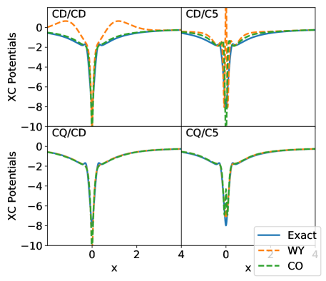
Figure 1: Neon atom XC potential from different combinations of OBS and PBS. BFGS runs for 30 iterations for all the results.

On the other hand, even though large basis sets for both the orbital and potential are preferred, this is impractical. A well-adopted strategy is to use a relatively small OBS to reduce the computational cost and to use a large and carefully chosen PBS to have a good representation for the potential. Following this strategy often introduces unphysical oscillations and thus regularization methods are required.

To better illustrate the limitations of finite basis sets and the sensitivity of the resulting potentials, we compare in Fig. 1 the XC potentials obtained for the Ne atom from WY and PDE-CO methods using different combinations of basis sets. The results are very sensitive to the choice of PBS and OBS. One could imagine that the unphysical features of the resulting XC potentials would depend strongly on the method used to perform the iKS. However, Fig.2 confirms that they are not. Even though the WY and PDE-CO methods are based on different principles, with optimizers traveling along different paths in the space spanned by the $\{\phi_{t}\}$, the unphysical features of the resulting XC potentials are largely the same, confirming the dominant role played by the finite basis sets.

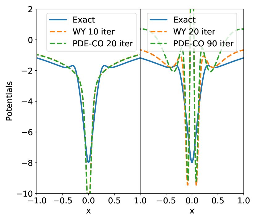
Figure 2: Ne atom XC potentials on CD/C5. BFGS is used with different number of iterations specified. The same initial point ($\{b_{t}\}=0$ and $v_{0}=v_{\rm FA}$) is used.

V Guide Potentials

The WY original method Wu and Yang (2003) uses the Fermi-Amaldi (FA) potentials Wu and Yang (2003); Zhao, Morrison, and Parr (1994)

$$v_{\rm FA}({\bf r})=\frac{N-1}{N}\int d{\bf r}^{\prime}\frac{n_{\rm in}({\bf r}^{\prime})}{|{\bf r}-{\bf r}^{\prime}|}$$ (20)

as a guide potential $v_{0}({\bf r})$ in Eq.(11), following Zhao, Morrison, and Parr Zhao, Morrison, and Parr (1994). Since the FA potential can be understood as a Hartree potential $v_{\scriptscriptstyle\rm H}({\bf r})=\int d{\bf r}^{\prime}\frac{n_{\rm in}({\bf r}^{\prime})}{|{\bf r}-{\bf r}^{\prime}|}$ with a part from exchange-correlation that partially prevents self-interaction, we also test $v_{0}({\bf r})=v_{\scriptscriptstyle\rm H}({\bf r})$ below. Because PBS usually has a poor behavior in the asymptotic region, $\sum_{t}b_{t}\phi_{t}({\bf r})$ often decays to $0$ too quickly (see Figure 3). In other words, $v_{0}({\bf r})$ should have the asymptotic behavior of $v_{\scriptscriptstyle\rm H}({\bf r})+v_{\scriptscriptstyle\rm XC}({\bf r})$ because $\sum_{t}b_{t}\phi_{t}({\bf r})$ has negligible contributions far from the nuclei. In the case of LDA densities, $v_{0}({\bf r})=v_{\scriptscriptstyle\rm H}({\bf r})$ fits this requirement better. However, the XC potentials obtained using $v_{0}({\bf r})=v_{\rm FA}({\bf r})$ usually have an asymptotic behavior that runs much closer to the exact one and leads to better satisfaction of Koopmans’ theorem, $\epsilon_{\rm HOMO}=-I$. This is true even when the LDA input density is used Wu, Ayers, and Yang (2003); Callow, Lathiotakis, and Gidopoulos (2020).

Figure 3: Neon atom XC potential and $\sum_{t}b_{t}\phi_{t}({\bf r})$ for different $v_{0}$ calculated in C5/C5. FA is Fermi-Amaldi and H is Hartree. The red dashed line is $y=0$.

VI Regularization

The effects of regularization are usually significant. The response function in (6) and the Hessian matrix in (14c) are supposed to sum over all unoccupied KS orbitals. The real response functions are invertible, but the Hessian matrices approximated with a finite number of KS orbitals are usually very singular, especially when the PBS differs significantly or is larger than the OBS Gidopoulos and Lathiotakis (2012), as shown in Fig. 4. truncated singular value decomposition (TSVD) regularization is thus often necessary. Wu and Yang used TSVD Hansen (1987) without providing a systematic way to determine the truncation threshold Wu and Yang (2003). Bulat et al. introduced an additional $\lambda$-regularizer

$$-\lambda\|{\nabla v_{\rm PBS}({\bf r})}\|^{2}\rightarrow-2\lambda\bm{b}^{T}{\bm{T}}\bm{b}$$ (21)

where $\bm{b}$ is the coefficient vector for $v_{\rm PBS}({\bf r})$ and ${\bm{T}}$ is the kinetic contribution to the Fock matrix Bulat et al. (2007). The L-curve method was introduced to search for the regularization parameter $\lambda$ Bulat et al. (2007); Heaton-Burgess and Yang (2008). Both methods are widely used as standard regularization for numerical optimization. They both contribute to the stability of the inversions irrespective of the basis-set employed and help overcome the over-fitting problems especially around the nuclei. To demonstrate this, we introduce here two simple but effective tricks: (1) Cliff-plotting to determine the optimum parameters for TSVD; and (2) $T_{s}$-focusing to optimize $\lambda$ for $\lambda$-regularization.

(1) The truncating parameters for TSVD depend on the systems and basis sets. The most straightforward method to determine these parameters is to plot the spectrum (the diagonal vector of the S matrix in SVD, see Figure 4). In many cases, the spectrum is of a “cliff” shape. Cutting at the edge of the cliff usually works. The main idea is to eliminate the subspace whose variations do not change the Fock matrices in Eq.(19). This simple method can be tricky when the OBS is much smaller than the PBS, where the spectrum shows several cliffs or disconnections and one has to decide on which one to cut. On the other hand, when the OBS and PBS are very close or the same, TSVD is often unnecessary. Moreover, optimizers like Trust-Krylov Gould et al. (1999) and L-BFGS Byrd et al. (1995) yield similar result as the Newton method with TSVD (Figure 4).

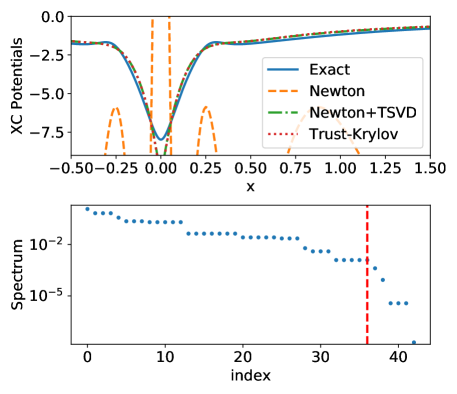
Figure 4: Neon atom XC potential using Newton+TSVD. The top panel shows results from different optimization methods. The bottom graph is the spectrum of singular values of the Hessian matrix before the convergence. The vertical red dashed line is the TSVD cutoff. CD/CT basis sets are used.

(2) Even with TSVD, there can still be over-fitting, especially around the nuclei (see Figure 4). We find that $\lambda$-regularization is more reliable in this region. In addition to the L-curve method introduced by Bulat et al. Bulat et al. (2007), we test here an alternative method to search for $\lambda$. We calculate $T_{s}(\lambda)$ as a function of $\lambda$ (see Figure 5). The point of $T_{s}(\lambda)$ with the largest $\lambda$ that is close enough to $T_{s}(\lambda=0)$ is chosen. The main idea is to adopt the simplest potential (corresponding to the largest $\lambda$) which does not essentially change the optimized result. Though obtaining $T_{s}(\lambda)$ curves such as those of Figs. 5-6 requires multiple inversion calculations, the efficiency of constrained optimization methods on finite PBS makes it acceptable in practice.

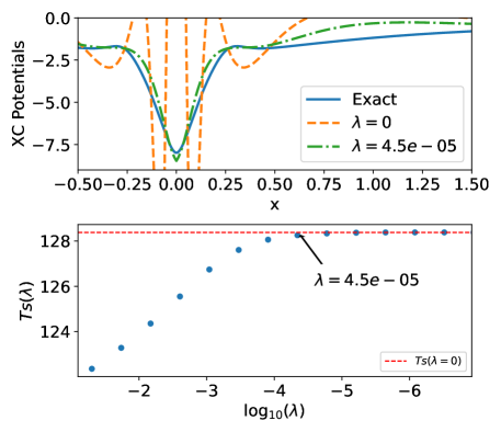
Figure 5: Neon atom XC potentials from the Wu-Yang method with $\lambda$-regularization. Newton with TSVD is used on CD/C5.

Motivated by the very similar overfitting features exhibited by the WY and PDE-CO methods, as evidenced in Fig.2, we now add $\lambda$-regularization to the Lagrangian of the PDE-CO method, Eq.(9). Note the sign for the regularization term needs to be changed when compared to (21) because (9) is minimized while (1) is concave for a given PBS. We follow a similar strategy to search for $\lambda$ as we have done for WY. Rather than $T_{s}(\lambda)$, the error (7) as a function of $\lambda$ is utilized and the largest $\lambda$ for a small enough error is selected (Fig. 6). In general it is impractical to search for a perfect $\lambda$ for a specific OBS/PBS. The simple method introduced above usually effectively eliminates the oscillations.

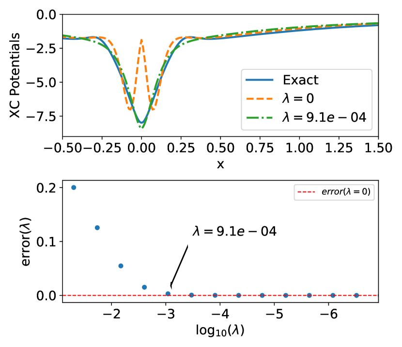
Figure 6: Neon atom XC potentials from the PDE-Constrained optimization with $\lambda$-regularization. $error(\lambda)$ is the density error function defined in (7). L-BFGS is used on CD/C5.

VII Null-Space Correction (NSC):

When using TSVD, it is possible that there is not a single clear edge and cutting at one edge does not lead to a smooth result. Also, cutting a Hessian matrix in this way “wastes” the large PBS selected. Instead of $\lambda$-regularization, a correction to the Hessian matrix can be defined based on the Unsöld approximation Unsöld (1927). This follows the derivation given by Gidopoulos and Lathiotakis Gidopoulos and Lathiotakis (2012) for OEP. When the Hessian information is used for the Wu-Yang method optimization, the following equation:

$${\bm{H}}_{0}\bm{b}_{0}=\bm{g}$$ (22)

is solved, where $\bm{b}_{0}$ is composed of the update coefficients for $v_{\rm PBS}({\bf r})$:

$$\begin{split}v^{k+1}_{\rm PBS}({\bf r})&=v^{k}_{\rm PBS}({\bf r})+\bigtriangleup v^{k}_{\rm 0,PBS}\\ &=v^{k}_{\rm PBS}({\bf r})+\sum_{t}b_{0,t}\phi_{t}({\bf r}),\end{split}$$ (23)

and $\bm{g}$ is the gradient vector. The null-space vector $\bar{\bm{b}}$ of the Hessian matrix ${\bm{H}}_{0}$ is added:

$${\bm{H}}_{0}(\bm{b}_{0}+\bar{\bm{b}})=\bm{g},$$ (24)

i.e. ${\bm{H}}_{0}\bar{\bm{b}}=0$. Now we define a $\bar{\bm{b}}$ that is a correction to $\bm{b}_{0}$ similar to the derivation by Gidopoulos and Lathiotakis Gidopoulos and Lathiotakis (2012), where the correction is derived for the Optimized Effective Potential.

The real response function $\chi({\bf r},{\bf r}^{\prime})$ is invertible; we denote the rest as $\tilde{\chi}({\bf r},{\bf r}^{\prime})$,

$$\tilde{\chi}({\bf r},{\bf r}^{\prime})=\chi({\bf r},{\bf r}^{\prime})-\chi_{0}({\bf r},{\bf r}^{\prime})$$ (25)

where $\chi_{0}$ is again the approximation summed over all the virtual orbitals in the KS-Slater determinant corresponding to ${\bm{H}}_{0}$ on finite basis sets. Using a short-hand notation in which $\chi\bigtriangleup\bm{v}$ stands for $\int d{\bf r}^{\prime}\chi({\bf r},{\bf r}^{\prime})\bigtriangleup\bm{v}({\bf r}^{\prime})$, we have

$$(\chi_{0}+\tilde{\chi})\bigtriangleup v=n-n_{\rm in}$$ (26)

and further

$$\chi_{0}\bigtriangleup v_{0}=n-n_{in},$$ (27)

The null-space vector $(\tilde{g}({\bf r}))$ can be separated from the right hand side, .i.e. $n({\bf r})-n_{in}({\bf r})=g({\bf r})+\tilde{g}({\bf r})$, where $\int d{\bf r}^{\prime}\chi_{0}({\bf r},{\bf r}^{\prime})\tilde{g}({\bf r}^{\prime})=0$. A parameter $\lambda$ is added to control the null-space component:

$$(\chi_{0}+\lambda\tilde{\chi})\bigtriangleup v^{\lambda}=g+\lambda\tilde{g}.$$ (28)

When $\lambda=1$, this is exactly (26). By setting $\lambda\rightarrow 0$, $\bigtriangleup v^{\lambda\rightarrow 0}$ can be derived. The null-space correction to $v_{0}({\bf r})$ is defined as difference between $\bigtriangleup v^{\lambda=0}({\bf r})$ and $\bigtriangleup v^{\lambda\rightarrow 0}({\bf r})$

$$\bigtriangleup\bar{v}({\bf r})=\bigtriangleup v^{\lambda\rightarrow 0}({\bf r})-\bigtriangleup v_{0}({\bf r}).$$ (29)

The discontinuity is shown as following. By setting $\lambda\rightarrow 0$, $\bigtriangleup v^{\lambda\rightarrow 0}({\bf r})$ can be expanded by orders of $\lambda$ using a Taylor series of $\bigtriangleup v^{\lambda}({\bf r})$ around $\lambda=0$, i.e. $\bigtriangleup v^{\lambda}({\bf r})=\bigtriangleup v^{\lambda\rightarrow 0}({\bf r})+\lambda\bigtriangleup v^{\prime}+\dots$. By matching the order of $\lambda$:

$$\mathcal{O}(1): \chi_{0}\bigtriangleup v^{\lambda\rightarrow 0}=g$$ (30a)

$$\mathcal{O}(\lambda): \chi_{0}\bigtriangleup v^{\prime}+\tilde{\chi}(\bigtriangleup\bar{v}+\bigtriangleup v_{0})=\tilde{g}.$$ (30b)

(30a) and (27) together prove that $\bigtriangleup\bar{v}$ is the null space vector of $\chi_{0}$.

By expanding all the potentials on the finite potential basis sets and integrating with the null-space vectors, the first term in (30b) disappears and it turns into matrix form:

$$({\bm{C}}^{\mu T}\tilde{{\bm{H}}})(\bm{b}_{0}+\bar{\bm{b}})={\bm{C}}^{\mu T}\bm{\tilde{g}}.$$ (31)

and

$${\bm{H}}_{0}\bm{c}^{\alpha} =\epsilon_{\alpha}\bm{c}^{\alpha}$$ (32a)

$${\bm{H}}_{0}\bm{c}^{\mu} =0.$$ (32b)

In order to do this, TSVD is used. We adopt the notation ${\bm{U}}^{\alpha},{\bm{V}}^{\alpha}$ and ${\bm{U}}^{\mu},{\bm{V}}^{\mu}$ for both $\epsilon^{\alpha}\leq\epsilon^{cutoff}$ and $\epsilon^{\mu}>\epsilon^{cutoff}$. $\bm{\tilde{g}}$ is $n({\bf r})-n_{\rm in}({\bf r})$ projection in the null space and integrated with the PBS:

$$\bm{\tilde{g}}={\bm{U}}^{\mu}{\bm{V}}^{\mu{\bm{T}}}\bm{g}$$ (33)

To approximate for $\tilde{{\bm{H}}}$, the Unsöld approximation Unsöld (1927) is adopted by setting the energy difference as a constant $C\simeq\epsilon_{a}-\epsilon_{i}$:

$$\begin{split}C\times\tilde{H}_{mn}=&\sum_{i}<\psi_{i}|\phi_{m}\phi_{n}|\psi_{i}>\\ &-\sum_{i}\sum_{p=\{i,a_{0}\}}<\psi_{i}|\phi_{m}|\psi_{p}><\psi_{p}|\phi_{n}|\phi_{i}>\end{split}$$ (34)

where $a_{0}$ denote the finite set of KS unoccupied orbitals. Since $\bar{v}({\bf r})$ is a null space function of $\chi_{0}$, it can be written as a linear combination of the null-space basis $\{u^{\nu}({\bf r})\}$:

$$\bar{\bm{b}}={\bm{V}}^{\mu}\bar{\bm{p}}$$ (35)

and one gets

$${\bm{U}}^{\mu T}\tilde{{\bm{H}}}{\bm{V}}^{\mu}\bar{\bm{p}}={\bm{U}}^{\mu T}\bm{\tilde{g}}-{\bm{U}}^{\mu T}\tilde{{\bm{H}}}\bm{b}_{0}$$ (36)

then

$$\bar{\bm{p}}={\bm{A}}^{-1}{\bm{U}}^{\mu T}\bm{\tilde{g}}-{\bm{A}}^{-1}{\bm{U}}^{\mu T}\tilde{{\bm{H}}}\bm{b}_{0}$$ (37)

where ${\bm{A}}={\bm{U}}^{\mu T}\tilde{{\bm{H}}}{\bm{V}}^{\mu}$. This is similar to Eq.(50) given by Gidopoulos and Lathiotakis Gidopoulos and Lathiotakis (2012). Because $\chi$ is supposed to be in general invertible, $\tilde{\chi}$’s projection into $\chi_{0}$’s null space, ${\bm{A}}$, should be invertible if the exact $\tilde{{\bm{H}}}$ is used. This is not usually true in practice. TSVD is often necessary for the inversion of ${\bm{A}}$. This correction fixes unphysical oscillations well, as shown in Fig. 7. This correction does not contribute in some cases, especially when the OBS and PBS are similar.

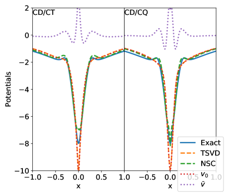
Figure 7: Neon atom potentials in CD/CT (left) and CD/CQ (right). TSVD and Null-Space Corrected (NSC) XC potentials are compared. $v_{0}$ is the original result and $\bar{v}$ is the correction term (i.e. ${\rm NSC}=v_{0}+\bar{v}$).

VIII Optimization Methods

The choice of optimization methods can also be important. Even for the WY method, which is concave, the optimized results can be very different with similar $T_{s}$ and density error (38) as we mentioned above. Here, we compare the performance of some of the most widely used methods that are available from the Scipy.optimize library Virtanen et al. (2020): quasi-Newton (BFGS Fletcher (2013), L-BFGS-B Byrd et al. (1995)), and trust-region methods (exact Conn, Gould, and Toint (2000), Krylov Gould et al. (1999)). We also implement Newton with TSVD regularization manually. As Wu and Yang pointed outWu and Yang (2003), the BFGS does not require TSVD and can often give a better convergence regarding $W[\Psi_{\rm det}[v_{\scriptscriptstyle\rm KS}],v_{\scriptscriptstyle\rm KS}]$ though more iterations are required.

We consider four different criteria including $W[\Psi_{\rm det}[v_{\rm KS}],v_{\rm KS}]$, $T_{s}[\Psi_{\rm det}]$, the gradient (13) norm $\|grad\|$ and density error

$$N_{error}=\int d{\bf r}|n({\bf r})-n_{\rm in}({\bf r})|.$$ (38)

The gradient norm $\|grad\|$ can be understood as metrics of optimization on a given PBS. The density error is more general and unlimited by the PBS. The gradient norm optimization is a necessary but insufficient condition for density error optimization because of the limitation of finite PBS (Table 3). The gradient norm is the main criterion used by optimizers for convergence.

Table 3: Two Different Norm Comparison at convergence.

Basis Set	CD/STO-3G		CD/CD		CD/CQ
	$\|grad\|$	$N_{error}$	$\|grad\|$	$N_{error}$	$\|grad\|$	$N_{error}$
Be	7.5e-6	1.8e-2	4.8e-5	1.6e-2	8.8e-7	4.2e-6
Ne	2.7e-6	3.1e-2	1.5e-5	7.8e-4	5.9e-5	1.5e-3
Ar	5.5e-8	9.2e-2	2.1e-6	6.8e-2	5.2e-5	4.7e-3

Table 4 and Figure 8 illustrate the performance of these different methods on the Ne atom. Trust-exact can still converge to a very overfitted potential when the PBS is not balanced. BFGS does not overcome the ill-condition of the accurate Hessian Matrix in extreme cases. L-BFGS-B, originally developed to save the memory for the Hessian matrices and maintaining a lower-rank approximated Hessian matrix, has a better performance than BFGS. Trust region methods and Newton’s method are more efficient than BFGS and L-BFGS-B as one can expect. In all the systems we tested, Trust-Krylov is the most robust method.

Table 4: Optimizer Performance for the Ne Atom^a

Method	$W[\Psi_{det},v_{KS}]$	$T_{s}[\Psi_{det}]$	$\|grad\|$b	$N_{error}$	$\epsilon_{\rm HOMO}$c	$N_{f}$d
Newtone+TSVD	128.609986	128.597	2.4e-2	4.9e-3	-0.6280	42
BFGS	128.609810	128.615	1.6e-3	8.1e-3	-0.7452	12
L-BFGS-B	128.609800	128.614	4.0e-3	7.5e-3	-0.7439	10
Trust-Exact	128.609948	128.593	1.5e-3	5.2e-3	-0.7010	3
Trust-Krylov	128.609926	128.609	6.6e-5	3.0e-3	-0.6988	4
Newton-CG	128.609823	128.605	2.2e-2	4.2e-3	-0.7408	5

^a Basis Set: CT/C5; ^b $L^{2}$; ^c The experimental I is 0.7925 West and Astle (1979);
^d the number of function evaluations; ^e Strong Wolfe line search is used.
PDE-CO: ^f3.5e-3; ^g-0.7460; ^h3.4e-3; ⁱ-0.7377.

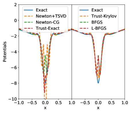
Figure 8: Neon atom XC potentials for common optimization methods in CT/C5.

IX Concluding Remarks

Pure density-to-potential iKS methods are in general more efficient but less accurate than wavefunction-based iKS methods. When implemented on finite PBS, with a further improvement on efficiency, the results are more sensitive. Based on our experience, some of which is shown in the Appendix Example Calculations, we recommend using the largest basis sets you can afford. Trust region methods, especially Trust-Krylov with $\lambda$-regularization, are usually more reliable (the search for $\lambda$ could start in a region $[10^{-4},10^{-6}]$). If a careful tuning is preferred, the Newton method with the null-space correction can be considered. Our code with all of the methods compared and discussed here will be open-sourced very soon, but a word of caution for the user is in order: pure iKS problems, especially with constrained optimizations, remain challenging. New ideas are needed.

X REFERENCES

References

- Hohenberg and Kohn (1964) P. Hohenberg and W. Kohn, “Inhomogeneous electron gas,” Physical review 136, B864 (1964).
- Kohn and Sham (1965) W. Kohn and L. J. Sham, “Self-consistent equations including exchange and correlation effects,” Physical review 140, A1133 (1965).
- Burke (2012) K. Burke, “Perspective on density functional theory,” The Journal of chemical physics 136, 150901 (2012).
- Verma and Truhlar (2020) P. Verma and D. G. Truhlar, “Status and challenges of density functional theory,” Trends in Chemistry 2, 302–318 (2020).
- Kurth and Perdew (2000) S. Kurth and J. P. Perdew, “Role of the exchange–correlation energy: Nature’s glue,” International Journal of Quantum Chemistry 77, 814–818 (2000).
- Nam et al. (2020a) S. Nam, R. J. McCarty, H. Park, and E. Sim, “Kohn-sham inversion toolkit,” arXiv preprint arXiv:2008.08783 (2020a).
- Unsleber et al. (2018) J. P. Unsleber, T. Dresselhaus, K. Klahr, D. Schnieders, M. Böckers, D. Barton, and J. Neugebauer, “Serenity: A subsystem quantum chemistry program,” (2018).
- Runge and Gross (1984) E. Runge and E. K. Gross, “Density-functional theory for time-dependent systems,” Physical Review Letters 52, 997 (1984).
- Helbig, Tokatly, and Rubio (2009) N. Helbig, I. V. Tokatly, and A. Rubio, “Exact kohn-sham potential of strongly correlated finite systems,” Journal of Chemical Physics 131 (2009).
- Hodgson et al. (2017) M. J. Hodgson, E. Kraisler, A. Schild, and E. K. Gross, “How interatomic steps in the exact kohn–sham potential relate to derivative discontinuities of the energy,” The journal of physical chemistry letters 8, 5974–5980 (2017).
- Thiele and Kummel (2009) M. Thiele and S. Kummel, “Photoabsorption spectra from adiabatically exact time-dependent density-functional theory in real time,” Physical Chemistry Chemical Physics 11, 4631–4639 (2009).
- Fuks et al. (2016) J. I. Fuks, S. E. B. Nielsen, M. Ruggenthaler, and N. T. Maitra, “Time-dependent density functional theory beyond kohn-sham slater determinants,” Physical Chemistry Chemical Physics 18, 20976–20985 (2016).
- Maitra et al. (2004) N. T. Maitra, F. Zhang, R. J. Cave, and K. Burke, “Double excitations within time-dependent density functional theory linear response,” Journal of Chemical Physics 120, 5932–5937 (2004).
- Maitra (2016) N. T. Maitra, “Perspective: Fundamental aspects of time-dependent density functional theory,” Journal of Chemical Physics 144 (2016), Artn 220901 10.1063/1.4953039.
- Nam et al. (2020b) S. Nam, S. Song, E. Sim, and K. Burke, “Measuring density-driven errors using kohn–sham inversion,” Journal of Chemical Theory and Computation 16, 5014–5023 (2020b).
- Naito, Ohashi, and Liang (2019) T. Naito, D. Ohashi, and H. Liang, “Improvement of functionals in density functional theory by the inverse kohn–sham method and density functional perturbation theory,” Journal of Physics B: Atomic, Molecular and Optical Physics 52, 245003 (2019).
- Accorto et al. (2020) G. Accorto, P. Brandolini, F. Marino, A. Porro, A. Scalesi, G. Colò, X. Roca-Maza, and E. Vigezzi, “First step in the nuclear inverse kohn-sham problem: From densities to potentials,” Physical Review C 101, 024315 (2020).
- Accorto et al. (2021) G. Accorto, T. Naito, H. Liang, T. Niksic, D. Vretenar, et al., “Nuclear energy density functionals from empirical ground-state densities,” Physical Review C 103, 044304 (2021).
- Brockherde et al. (2017) F. Brockherde, L. Vogt, L. Li, M. E. Tuckerman, K. Burke, and K.-R. Müller, “Bypassing the kohn-sham equations with machine learning,” Nature communications 8, 1–10 (2017).
- Nagai et al. (2018) R. Nagai, R. Akashi, S. Sasaki, and S. Tsuneyuki, “Neural-network kohn-sham exchange-correlation potential and its out-of-training transferability,” The Journal of chemical physics 148, 241737 (2018).
- Kalita et al. (2021) B. Kalita, L. Li, R. J. McCarty, and K. Burke, “Learning to approximate density functionals,” Accounts of Chemical Research , 253002 (2021).
- Manzhos (2020) S. Manzhos, “Machine learning for the solution of the schrödinger equation,” Machine Learning: Science and Technology 1, 013002 (2020).
- Jacob and Neugebauer (2014) C. R. Jacob and J. Neugebauer, “Subsystem density-functional theory,” Wiley Interdisciplinary Reviews-Computational Molecular Science 4, 325–362 (2014).
- Wesolowski, Shedge, and Zhou (2015) T. A. Wesolowski, S. Shedge, and X. W. Zhou, “Frozen-density embedding strategy for multilevel simulations of electronic structure,” Chemical Reviews 115, 5891–5928 (2015).
- Goodpaster et al. (2010) J. D. Goodpaster, N. Ananth, F. R. Manby, and T. F. Miller, “Exact nonadditive kinetic potentials for embedded density functional theory,” Journal of Chemical Physics 133 (2010).
- Nafziger, Wu, and Wasserman (2011) J. Nafziger, Q. Wu, and A. Wasserman, “Molecular binding energies from partition density functional theory,” Journal of Chemical Physics 135 (2011).
- Huang, Pavone, and Carter (2011) C. Huang, M. Pavone, and E. A. Carter, “Quantum mechanical embedding theory based on a unique embedding potential,” Journal of Chemical Physics 134 (2011).
- Kummel and Kronik (2008) S. Kummel and L. Kronik, “Orbital-dependent density functionals: Theory and applications,” Reviews of Modern Physics 80, 3–60 (2008).
- Levy (1979) M. Levy, “Universal variational functionals of electron densities, first-order density matrices, and natural spin-orbitals and solution of the v-representability problem,” Proceedings of the National Academy of Sciences 76, 6062–6065 (1979).
- Perdew et al. (2005) J. P. Perdew, A. Ruzsinszky, J. Tao, V. N. Staroverov, G. E. Scuseria, and G. I. Csonka, “Prescription for the design and selection of density functional approximations: More constraint satisfaction with fewer fits,” The Journal of chemical physics 123, 062201 (2005).
- Jin et al. (2017a) Y. Jin, Y. Yang, D. Zhang, D. G. Peng, and W. T. Yang, “Excitation energies from particle-particle random phase approximation with accurate optimized effective potentials,” Journal of Chemical Physics 147 (2017a), Artn 134105 10.1063/1.4994827.
- Jin et al. (2017b) Y. Jin, D. Zhang, Z. H. Chen, N. Q. Su, and W. T. Yang, “Generalized optimized effective potential for orbital functionals and self-consistent calculation of random phase approximations,” Journal of Physical Chemistry Letters 8, 4746–4751 (2017b).
- Flick et al. (2018) J. Flick, C. Schafer, M. Ruggenthaler, H. Appel, and A. Rubio, “Ab initio optimized effective potentials for real molecules in optical cavities: Photon contributions to the molecular ground state,” Acs Photonics 5, 992–1005 (2018).
- Yang and Wu (2002) W. Yang and Q. Wu, “Direct method for optimized effective potentials in density-functional theory,” Physical Review Letters 89, 143002 (2002).
- Gidopoulos and Lathiotakis (2012) N. I. Gidopoulos and N. N. Lathiotakis, “Nonanalyticity of the optimized effective potential with finite basis sets,” Physical Review A 85, 052508 (2012).
- Bulat et al. (2007) F. A. Bulat, T. Heaton-Burgess, A. J. Cohen, and W. Yang, “Optimized effective potentials from electron densities in finite basis sets,” The Journal of chemical physics 127, 174101 (2007).
- Heaton-Burgess and Yang (2008) T. Heaton-Burgess and W. Yang, “Optimized effective potentials from arbitrary basis sets,” The Journal of chemical physics 129, 194102 (2008).
- Aryasetiawan and Stott (1988) F. Aryasetiawan and M. Stott, “Effective potentials in density-functional theory,” Physical Review B 38, 2974 (1988).
- Görling (1992) A. Görling, “Kohn-sham potentials and wave functions from electron densities,” Physical Review A 46, 3753 (1992).
- Zhao and Parr (1992) Q. Zhao and R. G. Parr, “Quantities t s [n] and t c [n] in density-functional theory,” Physical Review A 46, 2337 (1992).
- Zhao and Parr (1993) Q. Zhao and R. G. Parr, “Constrained-search method to determine electronic wave functions from electronic densities,” The Journal of chemical physics 98, 543–548 (1993).
- Wang and Parr (1993) Y. Wang and R. G. Parr, “Construction of exact kohn-sham orbitals from a given electron density,” Physical Review A 47, R1591 (1993).
- Peirs, Van Neck, and Waroquier (2003) K. Peirs, D. Van Neck, and M. Waroquier, “Algorithm to derive exact exchange-correlation potentials from correlated densities in atoms,” Physical Review A 67, 012505 (2003).
- Kadantsev and Stott (2004) E. S. Kadantsev and M. Stott, “Variational method for inverting the kohn-sham procedure,” Physical Review A 69, 012502 (2004).
- Wagner et al. (2014) L. O. Wagner, T. E. Baker, E. Stoudenmire, K. Burke, and S. R. White, “Kohn-sham calculations with the exact functional,” Physical Review B 90, 045109 (2014).
- Ou and Carter (2018) Q. Ou and E. A. Carter, “Potential functional embedding theory with an improved kohn–sham inversion algorithm,” Journal of Chemical Theory and Computation 14, 5680–5689 (2018).
- Kumar, Singh, and Harbola (2019) A. Kumar, R. Singh, and M. K. Harbola, “Universal nature of different methods of obtaining the exact kohn–sham exchange-correlation potential for a given density,” Journal of Physics B: Atomic, Molecular and Optical Physics 52, 075007 (2019).
- Kumar and Harbola (2020) A. Kumar and M. K. Harbola, “A general penalty method for density-to-potential inversion,” International Journal of Quantum Chemistry 120, e26400 (2020).
- Ryabinkin, Kohut, and Staroverov (2015) I. G. Ryabinkin, S. V. Kohut, and V. N. Staroverov, “Reduction of electronic wave functions to kohn-sham effective potentials,” Physical review letters 115, 083001 (2015).
- Ospadov, Ryabinkin, and Staroverov (2017) E. Ospadov, I. G. Ryabinkin, and V. N. Staroverov, “Improved method for generating exchange-correlation potentials from electronic wave functions,” The Journal of chemical physics 146, 084103 (2017).
- Kumar, Singh, and Harbola (2020) A. Kumar, R. Singh, and M. K. Harbola, “Accurate effective potential for density amplitude and the correspondingkohn-sham exchange-correlation potential calculated from approximatewavefunctions,” Journal of Physics B: Atomic, Molecular and Optical Physics (2020).
- Zhao, Morrison, and Parr (1994) Q. Zhao, R. C. Morrison, and R. G. Parr, “From electron densities to kohn-sham kinetic energies, orbital energies, exchange-correlation potentials, and exchange-correlation energies,” Physical Review A 50, 2138 (1994).
- Wu, Ayers, and Yang (2003) Q. Wu, P. W. Ayers, and W. Yang, “Density-functional theory calculations with correct long-range potentials,” The Journal of chemical physics 119, 2978–2990 (2003).
- Nafziger, Jiang, and Wasserman (2017) J. Nafziger, K. Jiang, and A. Wasserman, “Accurate reference data for the nonadditive, noninteracting kinetic energy in covalent bonds,” Journal of chemical theory and computation 13, 577–586 (2017).
- Jensen and Wasserman (2018) D. S. Jensen and A. Wasserman, “Numerical methods for the inverse problem of density functional theory,” International Journal of Quantum Chemistry 118, e25425 (2018).
- Kanungo, Zimmerman, and Gavini (2019) B. Kanungo, P. M. Zimmerman, and V. Gavini, “Exact exchange-correlation potentials from ground-state electron densities,” Nature communications 10, 1–9 (2019).
- Callow, Lathiotakis, and Gidopoulos (2020) T. J. Callow, N. N. Lathiotakis, and N. I. Gidopoulos, “Density-inversion method for the kohn–sham potential: Role of the screening density,” The Journal of chemical physics 152, 164114 (2020).
- Hadamard (1902) J. Hadamard, “Sur les problèmes aux dérivées partielles et leur signification physique,” Princeton university bulletin , 49–52 (1902).
- Chayes, Chayes, and Ruskai (1985) J. Chayes, L. Chayes, and M. B. Ruskai, “Density functional approach to quantum lattice systems,” Journal of statistical physics 38, 497–518 (1985).
- Ullrich and Kohn (2002) C. Ullrich and W. Kohn, “Degeneracy in density functional theory: Topology in the v and n spaces,” Physical review letters 89, 156401 (2002).
- Lammert (2006) P. E. Lammert, “Coarse-grained v representability,” The Journal of chemical physics 125, 074114 (2006).
- Li et al. (2020) L. Li, S. Hoyer, R. Pederson, R. Sun, E. D. Cubuk, P. Riley, and K. Burke, “Kohn-sham equations as regularizer: building prior knowledge into machine-learned physics,” arXiv preprint arXiv:2009.08551 (2020).
- Nagai, Akashi, and Sugino (2020) R. Nagai, R. Akashi, and O. Sugino, “Completing density functional theory by machine learning hidden messages from molecules,” npj Computational Materials 6, 1–8 (2020).
- Gaiduk, Ryabinkin, and Staroverov (2013) A. P. Gaiduk, I. G. Ryabinkin, and V. N. Staroverov, “Removal of basis-set artifacts in kohn–sham potentials recovered from electron densities,” Journal of chemical theory and computation 9, 3959–3964 (2013).
- Wu and Yang (2003) Q. Wu and W. Yang, “A direct optimization method for calculating density functionals and exchange–correlation potentials from electron densities,” The Journal of chemical physics 118, 2498–2509 (2003).
- Jacob (2011) C. R. Jacob, “Unambiguous optimization of effective potentials in finite basis sets,” The Journal of chemical physics 135, 244102 (2011).
- Vogel (2002) C. R. Vogel, Computational methods for inverse problems (SIAM, 2002).
- Umrigar and Gonze (1994) C. J. Umrigar and X. Gonze, “Accurate exchange-correlation potentials and total-energy components for the helium isoelectronic series,” Physical Review A 50, 3827 (1994).
- Filippi, Gonze, and Umrigar (1996) C. Filippi, X. Gonze, and C. Umrigar, “Recent developments and applications of modern density functional theory,” (1996).
- Parrish et al. (2017) R. M. Parrish, L. A. Burns, D. G. Smith, A. C. Simmonett, A. E. DePrince III, E. G. Hohenstein, U. Bozkaya, A. Y. Sokolov, R. Di Remigio, R. M. Richard, et al., “Psi4 1.1: An open-source electronic structure program emphasizing automation, advanced libraries, and interoperability,” Journal of chemical theory and computation 13, 3185–3197 (2017).
- Smith et al. (2018) D. G. Smith, L. A. Burns, D. A. Sirianni, D. R. Nascimento, A. Kumar, A. M. James, J. B. Schriber, T. Zhang, B. Zhang, A. S. Abbott, et al., “Psi4numpy: An interactive quantum chemistry programming environment for reference implementations and rapid development,” Journal of chemical theory and computation 14, 3504–3511 (2018).
- Wu (2014) Q. Wu, “Variational nature of the frozen density energy in density-based energy decomposition analysis and its application to torsional potentials,” The Journal of Chemical Physics 140, 244109 (2014).
- Baydin et al. (2018) A. G. Baydin, B. A. Pearlmutter, A. A. Radul, and J. M. Siskind, “Automatic differentiation in machine learning: a survey,” Journal of machine learning research 18 (2018).
- Mura, Knowles, and Reynolds (1997) M. E. Mura, P. J. Knowles, and C. A. Reynolds, “Accurate numerical determination of kohn-sham potentials from electronic densities: I. two-electron systems,” The Journal of chemical physics 106, 9659–9667 (1997).
- Schipper, Gritsenko, and Baerends (1997) P. Schipper, O. Gritsenko, and E. Baerends, “Kohn-sham potentials corresponding to slater and gaussian basis set densities,” Theoretical Chemistry Accounts 98, 16–24 (1997).
- Staroverov, Scuseria, and Davidson (2006) V. N. Staroverov, G. E. Scuseria, and E. R. Davidson, “Optimized effective potentials yielding hartree–fock energies and densities,” (2006).
- Hansen (1987) P. C. Hansen, “The truncatedsvd as a method for regularization,” BIT Numerical Mathematics 27, 534–553 (1987).
- Gould et al. (1999) N. I. Gould, S. Lucidi, M. Roma, and P. L. Toint, “Solving the trust-region subproblem using the lanczos method,” SIAM Journal on Optimization 9, 504–525 (1999).
- Byrd et al. (1995) R. H. Byrd, P. Lu, J. Nocedal, and C. Zhu, “A limited memory algorithm for bound constrained optimization,” SIAM Journal on scientific computing 16, 1190–1208 (1995).
- Unsöld (1927) A. Unsöld, “Quantentheorie des wasserstoffmolekülions und der born-landéschen abstoßungskräfte,” Zeitschrift für Physik 43, 563–574 (1927).
- Virtanen et al. (2020) P. Virtanen, R. Gommers, T. E. Oliphant, M. Haberland, T. Reddy, D. Cournapeau, E. Burovski, P. Peterson, W. Weckesser, J. Bright, et al., “Scipy 1.0: fundamental algorithms for scientific computing in python,” Nature methods 17, 261–272 (2020).
- Fletcher (2013) R. Fletcher, Practical methods of optimization (John Wiley & Sons, 2013).
- Conn, Gould, and Toint (2000) A. R. Conn, N. I. Gould, and P. L. Toint, Trust region methods (SIAM, 2000).
- West and Astle (1979) R. C. West and M. J. Astle, “Crc handbook of chemistry and physics,” CRC Process, Boca Raton, Fl, 1987), p. D-71 (1979).