The gradient descent method for the convexification to solve boundary value problems of quasi-linear PDEs and a coefficient inverse problem

Abstract

We study the global convergence of the gradient descent method of the minimization of strictly convex functionals on an open and bounded set of a Hilbert space. Such results are unknown for this type of sets, unlike the case of the entire Hilbert space. Then, we use our result to establish a general framework to numerically solve boundary value problems for quasi-linear partial differential equations (PDEs) with noisy Cauchy data. The procedure involves the use of Carleman weight functions to convexify a cost functional arising from the given boundary value problem and thus to ensure the convergence of the gradient descent method above. We prove the global convergence of the method as the noise tends to 0. The convergence rate is Lipschitz. Next, we apply this method to solve a highly nonlinear and severely ill-posed coefficient inverse problem, which is the so-called back scattering inverse problem. This problem has many real-world applications. Numerical examples are presented.

Key words: boundary value problem, quasi-linear, convexification, gradient descent method, coefficient inverse problem.

AMS subject classification: 35R25, 35N10, 35R30, 78A46

1 Introduction

Numerical solutions of ill-posed Cauchy problems for quasi-linear partial differential equations (PDEs) is an important topic that arises in many real-world applications. For example, in the case of parabolic PDEs such problems are common in heat conduction [1, 2]. A natural approach to solve such a problem is to minimize the functional defined by the least-squares method. However, due to the presence of the nonlinearity, this functional is non convex. It might have multiple local minima and ravines. Therefore, a good initial guess, which is located sufficiently close to the true solution, plays an important role in the minimization process. Since such a good initial guess is not always available, we, in this paper, use the convexification method, in which it is not necessary to have a small distance between the starting point of iterations and the true solution. The main content of the convexification method is to construct a weighted cost functional, which is strictly convex on an a priori chosen bounded set. It is important that smallness condition is not imposed on the diameter of this set. The unique minimizer of that functional on that set is close to the true solution of the given ill-posed Cauchy problem. The key element of that functional is the Carleman Weight Function (CWF), which is involved as weight in the Carleman estimate for the corresponding PDE operator.

An important question arises immediately on how to efficiently find the global minimizer of such a convex functional on that bounded set. It is well known that if a functional is strictly convex on the whole Hilbert space, then the gradient descent method converges to its unique minimizer if starting from an arbitrary point of that space. However, it is not clear what to do in our case when the strict convexity takes place only on a bounded set. To address this question, it was proposed in [3] to use the gradient projection method. However, this method is a complicated one and is hard to implement numerically. On the other hand, it was heuristically observed in all numerical studies of the convexification conducted so far that a simpler gradient descent method works well; see e.g., [3, 8, 9, 10, 18]. This motivates us to analytically study the question of the global convergence of the gradient descent method.

More precisely, we prove that the gradient descent method delivers a sequence converging to the minimizer of that functional on that bounded set if starting from an arbitrary point of that set. Since smallness conditions are not imposed on the diameter of this set, this is global convergence, see, e.g. [3] where the notion of global convergence is defined. Some numerical results by gradient descent method will be presented.

Another important part of this paper is to apply this result to solve a highly nonlinear and severely ill-posed coefficient inverse problem with a single measurement of back scattering data in the frequency domain.

As mentioned above, the main idea of the convexification method is to construct a strictly convex functional. To do this, one uses the Carleman weight function to convexify the mismatch functional derived from the given boundary value problem. Several versions of the convexification method have been developed since it was first introduced in [16]. We cite here [14, 12, 3, 19, 10, 20] for some important works in this area and their applications to solve a variety kinds of inverse problems. A comprehensive study of the convexification method is presented in the recent published book [18]. The crucial mathematical results that guarantee the above mentioned properties of the convexification, are the Carleman estimates. The original idea of applying Carleman estimates to coefficient inverse problems was first published in [5] back in 1981 to prove uniqueness theorems for a wide class of coefficient inverse problems. Some follow up publications can be found in, e.g. [22, 11, 7, 27, 24, 30]. Surveys on the method in [5] can be found in [13, 33], see also [4, Chapter 1] and [18]. It was discovered later in [16], that the idea of [5] can be successfully modified to develop globally convergent numerical methods for coefficient inverse problems using the convexification.

For the convenience of the reader, we will recall in this paper the convexification method , to solve ill-posed Cauchy problems for quasi-linear PDEs with both Dirichlet and Neumann boundary data [14]. Then, we will prove that if the noise in the boundary data tends to zero, then the convexification method combined with the gradient descent method delivers a close approximation to the solution of that Cauchy problem if starting from an arbitrary point of a selected bounded set. The rate of convergence is Lipschitz. We next apply the above results to solve a highly nonlinear and severely ill-posed coefficient inverse problem, described below. At a point far away from the region of interest, we send out an incident electric wave. The incident wave propagates in the 3D space and scatters when hitting the targets. We measure the back scattering wave on a surface. The aim of the inverse problem is to reconstruct the spatially distributed dielectric constants from this measurement. This coefficient inverse problem is the so-called inverse back scattering problem. It has many real-world applications, including the detection and identification of explosives, nondestructive testing and material characterization, see [9, 8, 29, 32]. We also refer the reader to [6] for the applications of this coefficient inverse problem in sonar imaging, geographical exploration, medical imaging, near-field optical microscopy, nano-optics.

The widely-used method to solve nonlinear coefficient inverse problem is the least squares optimization. This approach requires a good initial guess of the true solution. Unlike this, we assume that the target to be detected is completely unknown. This means that a good initial guess of its dielectric constant is unavailable. Our numerical procedure is as follows. We first eliminate the unknown dielectric constant from the governing Helmholtz equation. The obtained equation is not a standard PDE. Then, we approximate the solution of the latter PDE via a truncated Fourier series with respect to a special orthonormal basis. Then we obtain an ill-posed Cauchy problem for a coupled system of elliptic of PDEs wih respect to corresponding spatially dependent Fourier coefficients. That special orthonormal basis was originally introduced in [15]. Solving this system by the convexification method and the gradient descent method, we obtain the solution to the above non standard PDE above. Then the solution to the originating coefficient inverse problem follows. We refer the reader to [8, 10, 31] and the references therein for some related versions of this method.

The paper is organized as follows. In Section 2, we prove the convergence of the gradient descent method to the minimizer of a strictly convex functional. In Section 3, we present the above mentioned ill-posed Cauchy problem for a quasilinear elliptic PDE with both Dirichlet and Neumann boundary conditions. Also, in this section we present the corresponding functional with the Carleman Weight Function in it. In section 4, we recall the convexification method. In this section, we also prove the Lipschitz-like convergence of the minimizers due to the convexification method to the true solution as the noise tends to zero. In section 5, we introduce our coefficient inverse problem. In section 6, we derive an approximate model to solve this coefficient inverse problem. We present some numerical examples in section 7. Section 8 is for concluding remarks.

2 The gradient descent method to minimize a convex functional

Let $X$ be a Hilbert space and let $J:X\rightarrow\mathbb{R}$ be a functional. Assume that $J$ is Fréchet differentiable. Its derivative at the point $v\in X$ is denoted by $DJ(v):X\rightarrow\mathbb{R}$. By the Riesz representation theorem, for each $v\in X,$ we can identify $DJ(v)$ with an element of $X$, named as $J^{\prime}(v),$ in the following sense

$$DJ(v)(h)=\langle J^{\prime}(v),h\rangle_{X}\quad\mbox{for all }h\in X.$$

Let $M>0$ be an arbitrary number. Consider the ball $B\left(M\right),$

$$B\left(M\right)=\left\{v\in X:\left\|v\right\|_{X}<M\right\}.$$

We assume that the Fréchet derivative $J^{\prime}$ is Lipschitz continuous in $\overline{B\left(M\right)},$ i.e.

$$\left\|J^{\prime}(v_{2})-J^{\prime}(v_{1})\right\|_{X}\leq L\left\|v_{2}-v_{1}\right\|_{X},\text{ }\forall v_{1},v_{2}\in\overline{B\left(M\right)},$$ (2.1)

where $L$ is a certain number. Assume that $J$ is strictly convex on $\overline{B\left(M\right)}$. This means that there exists a constant $\Lambda>0$ such that

$$\langle J^{\prime}(v_{1})-J^{\prime}(v_{2}),v_{1}-v_{2}\rangle_{X}\geq\Lambda\|v_{1}-v_{2}\|_{X}^{2}\quad\mbox{for all }v_{1},v_{2}\in\overline{B\left(M\right)}.$$ (2.2)

Theorem 2.1 follows from a combination of Lemma 2.1 and Theorem 2.1 of [3].

Theorem 2.1

Assume that the functional $J:X\rightarrow\mathbb{R}$ is Fréchet differentiable on $X$ and its Fréchet derivative is Lipschitz continuous on $\overline{B(M)}$ as in (2.1). Also, assume that $J\left(v\right)$ is strictly convex in $\overline{B(M)}$; i.e., inequality (2.2) is true. Then there exists unique minimizer $v_{\mathrm{min}}\in\overline{B\left(M\right)}$ of the functional $J\left(v\right)$ on the set $\overline{B\left(M\right)},$

$$\min_{\overline{B\left(M\right)}}J\left(v\right)=J\left(v_{\mathrm{min}}\right).$$

Furthermore, the following inequality holds

$$\langle J^{\prime}\left(v_{\mathrm{min}}\right),v_{\mathrm{min}}-y\rangle_{X}\leq 0,\quad\mbox{for all }y\in\overline{B\left(M\right)}.$$

The fact that the minimizer guaranteed by Theorem 2.1 can be located on the boundary of the ball $\overline{B(M)}$ prevents us from the proof of the global convergence of the gradient descent method. Hence, we assume in the next theorem that the minimizer is an interior point of $B(M).$

Theorem 2.2

Assume that the functional $J:X\rightarrow\mathbb{R}$ satisfies conditions of Theorem 2.1. Let $v_{\mathrm{min}}$ be its minimizer on the set $\overline{B\left(M\right)},$ the uniqueness and existence of which is guaranteed by Theorem 2.1. Suppose that $v_{\mathrm{min}}$ belongs to the interior of $B\left(M\right).$ Fix $v^{(0)}\in B$. Assume that the ball centered at $v_{\mathrm{min}}$ with the radius $\|v^{(0)}-v_{\mathrm{min}}\|_{X}$ is contained in $B\left(M\right);$ i.e.,

$$B_{0}=B(v_{\mathrm{min}},\|v^{(0)}-v_{\mathrm{min}}\|_{X})\subset B\left(M\right).$$ (2.3)

Denote $\eta_{0}=\min\left(2\Lambda/L^{2},1\right)$ and fix $\eta\in(0,\eta_{0}).$ For each $m\geq 0,$ define

$$v^{(m+1)}=v^{(m)}-\eta J^{\prime}\big{(}v^{(m)}\big{)},\quad m\geq 1$$ (2.4)

Then, there exists a number $q\in\left(0,1\right)$ such that

$$v^{(m)}\in B(M)\quad\mbox{and }\big{\|}v^{m}-v_{\min}\big{\|}_{X}\leq q^{m-1}\big{\|}v^{(0)}-v_{\min}\big{\|}_{X},\quad m\geq 1.$$ (2.5)

As a result, the sequence $v^{(m)}$ converges to $v_{\rm min}$ as $m$ tends to $\infty.$

The sequence $\{v^{(m)}\}_{m\geq 1}$ defined in (2.4) is generated by the well-known gradient descent method. Although the gradient descent method is widely used in the scientific community, its convergence for a nonconvex functional can be proven only if the starting point of iterations is sufficiently close to the minimizer. Unlike this, Theorem 2.2 provides an affirmative answer about the convergence when the starting point is not necessary located in a sufficiently small neighborhood of the minimizer. Theorem 2.2 justifies recent numerical results of our research group where we have used the gradient descent method to minimize globally strictly convex cost functionals arising in convexification even though our past theory said that a more complicated gradient projection method should be used, see e.g., [3, 8, 9, 10, 18, 20].

Proof of Theorem 2.2. Let $L$ and $\Lambda$ be the constants in (2.1) and (2.2) respectively and let $q=1+\eta^{2}L^{2}-2\eta\Lambda$. Since $\eta\in(0,\eta_{0}),$ $q\in(0,1).$ We prove (2.5) by induction. Assume, by induction, that (2.5) is true for some $m\geq 1$. Due to assumption (2.3), $v_{\min}\in B\left(M\right).$ Thus, $J^{\prime}(v_{\min})=0.$ Hence, $v_{\min}=v_{\min}-J^{\prime}\left(v_{\min}\right).$ By (2.4), we have

$$\|v^{(m+1)}-v_{\min}\|_{X}^{2} =\|v^{(m)}-v_{\min}-\eta(J^{\prime}\left(v^{(m)}\right)-J^{\prime}(v_{\min}))\|_{X}^{2}$$

$$=\|v^{(m)}-v_{\min}\|_{X}^{2}+\eta^{2}\|J^{\prime}\left(v^{(m)}\right)-J^{\prime}(v_{\min})\|_{X}^{2}$$

$$\hskip 71.13188pt-2\eta\langle J^{\prime(m)})-J^{\prime}(v_{\min}),v^{(m)}-v_{\min}\rangle_{X}.$$

Using this, together with (2.1), (2.2) and the induction assumption for (2.5), we obtain

$$\|v^{(m+1)}-v_{\min}\|_{X}^{2}\leq q\|v^{(m)}-v_{\min}\|_{X}^{2}\leq q^{m}\|v^{(0)}-v_{\min}\|_{X}^{2}.$$ (2.6)

The last inequality in (2.6) is deduced from the induction hypothesis. It follows from (2.6) that $v^{(m+1)}\in B_{0}\subset B$. The assertion (2.5) is proved. $\square$

Remark 1

1. The hypothesis that the starting point of iterations $v^{(0)}$ is such that the ball centered at $v_{\mathrm{min}}$ with the radius $\|v_{\min}-v_{0}\|_{X}$ is contained in $B\left(M\right)$ does not weaken Theorem 2.2. In fact, if this hypothesis is not satisfied, we can replace $B\left(M\right)$ by a larger ball $B\left(M^{\prime}\right)$ where $M^{\prime}>M.$ Note that in the convexification method, $B\left(M\right)$ is the ball with an arbitrary chosen radius.

2. The assumption that $v_{\mathrm{min}}$ is inside $B\left(M\right)$ is the main reason that helps us to replace the gradient projection method in [9, 10, 8, 3] with the gradient descent method in Theorem 2.2. Without this assumption, elements of the sequence produced by the gradient descent method might be outside of $B\left(M\right)$, thus making this sequence diverge.

3. We refer the reader to [17, Theorem 6], in which the authors proved a less general case of Theorem 2.2.

3 A boundary value problem for quasi-linear PDEs

Let $n\geq 2$ be the spatial dimension. Let $\Omega$ be an open and bounded domain in $\mathbb{R}^{n}$ and $\Gamma$ be a part of $\partial\Omega.$ Let $G:\Omega\times\mathbb{R}\times\mathbb{R}^{n}\rightarrow\mathbb{R}$ be a real value function in the class $C^{2}(\overline{\Omega}\times\mathbb{R}\times\mathbb{R}^{n},\mathbb{R})$. Consider the following boundary value problem with both Dirichlet and Neumann boundary conditions

$$\left\{\begin{array}[]{rcll}\Delta v(\mathbf{x})&=&G(\mathbf{x},v(\mathbf{x}),\nabla v(\mathbf{x}))&\mathbf{x}\in\Omega,\\ \partial_{\nu}v(\mathbf{x})&=&g_{0}(\mathbf{x})&\mathbf{x}\in\Gamma,\\ v(\mathbf{x})&=&g_{1}(\mathbf{x})&\mathbf{x}\in\partial\Omega\end{array}\right.$$ (3.1)

where $g_{0}$ and $g_{1}$ are two functions in the class $H^{p}(\Omega)$ where $p$ is a positive integer with $p>\lceil n/2\rceil+2.$ In fact, we can say that (3.1) is the Cauchy problem for a quasilinear elliptic equation with the additional Dirichlet boundary data at $\partial\Omega\diagdown\Gamma.$ Here, $\lceil n/2\rceil$ is the smallest integer that is greater than $n/2$. This regularity condition guarantees the embedding $H^{p}(\Omega)\hookrightarrow C^{2}(\overline{\Omega})$. This embedding will be used for the regularization purpose. In practice, the functions $g_{0}$ and $g_{1}$ represent the flux and the value information of $v$ on $\partial\Omega$ and $\Gamma$ respectively. We first recall the convexification method to compute an approximation of the solution, if exists, to (3.1). Suppose that

$$H=\{\phi\in H^{p}(\Omega):\partial_{\nu}\phi(\mathbf{x})=g_{0}(\mathbf{x})\mbox{ for all }\mathbf{x}\in\Gamma\mbox{ and }\phi(\mathbf{x})=g_{1}(\mathbf{x})\mbox{ for all }\mathbf{x}\in\partial\Omega\}$$ (3.2)

is nonempty. Let $v_{0}$ be a function in $H$. Define

$$u(\mathbf{x})=v(\mathbf{x})-v_{0}(\mathbf{x})\quad\mbox{for all }\mathbf{x}\in\Omega.$$ (3.3)

Then, solving (3.1) is equivalent to solving

$$\left\{\begin{array}[]{rcll}\Delta u(\mathbf{x})&=&F(\mathbf{x},u(\mathbf{x}),\nabla u(\mathbf{x}))&\mathbf{x}\in\Omega,\\ \partial_{\nu}u(\mathbf{x})&=&0&\mathbf{x}\in\Gamma,\\ u(\mathbf{x})&=&0&\mathbf{x}\in\partial\Omega\end{array}\right.$$ (3.4)

where

$$F(\mathbf{x},s,\xi)=\Delta v_{0}(\mathbf{x})+G(\mathbf{x},s+v_{0}(\mathbf{x}),\xi+\nabla v_{0}(\mathbf{x}))$$ (3.5)

for all $\mathbf{x}\in\Omega,s\in\mathbb{R},\xi\in\mathbb{R}^{n}$. Let

$$H_{0}=\big{\{}\phi\in H^{p}(\Omega):\partial_{\nu}\phi(\mathbf{x})=0\mbox{ for all }\mathbf{x}\in\Gamma\mbox{ and }\phi(\mathbf{x})=0\mbox{ for all }\mathbf{x}\in\partial\Omega\big{\}}.$$ (3.6)

It is obvious that $H_{0}$ is a closed subspace of $H^{p}(\Omega)$. We consider $H_{0}$ a Hilbert space endowed with the usual norm of $H^{p}(\Omega).$ A widely-used approach to solve (3.4) is to minimize the following least squares functional

$$\int_{\Omega}\big{|}\Delta u(\mathbf{x})-F\big{(}\mathbf{x},u(\mathbf{x}),\nabla u(\mathbf{x})\big{)}\big{|}^{2}d\mathbf{x}+\mbox{a regularization term}.$$ (3.7)

for $u\in H_{0}.$ Due to the nonlinearity of $F$, and hence $L$, the functional in (3.7) is nonconvex. It might have multiple local minima and ravines, making the direct optimization approach unpractical. Motivated by this fact, we “convexify” this functional using the idea in [15]. Let $\Psi:\Omega\rightarrow\mathbb{R}$ be a $C^{\infty}$ function with $\nabla\Psi\not=0$ for all $\mathbf{x}\in\overline{\Omega}.$ Introduce the Carleman weight function

$$\mu_{\lambda}(\mathbf{x})=\exp(2\lambda\Psi(\mathbf{x}))\quad\mbox{for all }\mathbf{x}\in\Omega$$ (3.8)

where $\lambda>1$. A Carleman estimate is an inequality of the form below.

Assumption 1 (Carleman estimate)

There exists $\lambda_{0}>1$ depending only on $\Omega$ and $n$ such that for all $\phi\in H^{2}(\Omega)$ with $\phi|_{\partial\Omega}=0$ and $\partial_{\nu}\phi|_{\Gamma}=0$, we have

$$\int_{\Omega}\mu_{\lambda}(\mathbf{x})|\Delta\phi|^{2}d\mathbf{x}\geq\frac{C}{\lambda}\sum_{i,j=1}^{n}\int_{\Omega}\mu_{\lambda}(\mathbf{x})|\partial_{x_{i}x_{j}}\phi(\mathbf{x})|^{2}d\mathbf{x}+C\lambda\int_{\Omega}\mu_{\lambda}(\mathbf{x})[|\nabla\phi|^{2}+\lambda^{2}|\phi|^{2}]d\mathbf{x}$$ (3.9)

for all $\lambda\geq\lambda_{0}$ for some positive constant $C$ depending only on $\Omega$.

Assumption 1 holds true for some functions $\Psi$ and $\mu_{\lambda}$. For example, Klibanov and his collaborators have established a Carleman estimate in [19, Theorem 4.1], in which $\Omega=(-R,R)^{3}\subset\mathbb{R}^{3}$ for some $R>0$ and $\Psi(x,y,z)=(z-r)^{2}$ where $r$ is any number that is greater than $R$. On the other hand, following the arguments in [19, Theorem 4.1], one can prove a Carleman estimate with $\Psi(x,y,z)=(z+r)^{2}$, see [10, Theorem 3.1]. This estimate plays an important role in developing a numerical method to solve the back scattering inverse problem with moving point source in [10]. On the other hand, the reader can find another Carleman estimate in [24, Theorem 3.1] when the second derivatives of the test function $\phi$ are absence in the right hand side of (3.9). We also cite to [4, 18] for some important versions of Carleman estimate for other kinds of partial differential operators. Especially, we draw the reader’s attention to [5] for the original idea of using Carleman estimate to prove the uniqueness of a variety kinds of inverse problems.

Without lost of the generality, we assume that the true solution to (3.4) has a finite $H^{p}(\Omega)$-norm, which is bounded from above by a known number $M$. We seek this solution in the set

$$B(M)=\big{\{}\phi\in H_{0}:\|\phi\|_{H^{p}(\Omega)}<M\big{\}}.$$ (3.10)

More precisely, in order to find a numerical solution to (3.4), we solve the problem below.

Problem 3.1

Fix a regularization parameter $\epsilon>0$. Minimize the following functional

$$J_{\epsilon,\lambda}(u)=\int_{\Omega}\mu_{\lambda}(\mathbf{x})\big{|}\Delta u(\mathbf{x})-F\big{(}\mathbf{x},u(\mathbf{x}),\nabla u(\mathbf{x})\big{)}\big{|}^{2}d\mathbf{x}+\epsilon\|u\|^{2}_{H^{p}(\Omega)}$$ (3.11)

for all $u\in B(M)$.

In the next section, we will recall the convexification principle to solve Problem 3.1. The main content of the convexification principle is that if the Carleman estimate (3.9) holds true then for any arbitrarily large number $M$, there exists $\lambda_{1}>\lambda_{0}$ such that for all $\lambda>\lambda_{1}$ and $\epsilon>0,$ $J_{\epsilon,\lambda}$ is strictly convex in $\overline{B(M)}$ where $B(M)$ is the ball in $H_{0}$ with center $0$ and radius $M$, see (3.10).

4 The convexification method and the convergence of the minimizer to the true solution as the noise tends to zero

In this section, we recall a theorem (Theorem 4.1) that guarantees the convexity of the objective functional $J_{\epsilon,\lambda}$ in $\overline{B(M)}$. We write $F=F(\mathbf{x},s,\xi)$ and the partial derivatives of $F(\mathbf{x},s,\xi)$ with respect to its variables are written as $\nabla_{\mathbf{x}}F(\mathbf{x},s,\xi),$ $\partial_{s}F(\mathbf{x},s,\xi)$ and $\nabla_{\xi}F(\mathbf{x},s,\xi)$. The following theorem, Theorem 4.1, guarantees that $J_{\epsilon,\lambda}$ has Lipschitz continuous Fréchet derivative and, more importantly, that $J_{\epsilon,\lambda}$ is strictly convex if the Carleman weight function $\mu_{\lambda}$ is such that Assumption 1 holds true.

Theorem 4.1 (Convexification)

1. Let $M$ be an arbitrary positive number and define the ball $B(M)$ as in (3.10). Then, for all $\epsilon>0$ and $\lambda>1$, $J_{\epsilon,\lambda}:\overline{B(M)}\subset H_{0}\to\mathbb{R}$ is Fréchet differentiable. The derivative of $J_{\epsilon,\lambda}$ is given by

$$DJ_{\epsilon,\lambda}(u)h=2\int_{\Omega}\mu_{\lambda}(\mathbf{x})\big{(}\Delta u(\mathbf{x})-F(\mathbf{x},u(\mathbf{x}),\nabla u(\mathbf{x}))\big{)}\big{(}\Delta h(\mathbf{x})-DF(u)h(\mathbf{x})\big{)}d\mathbf{x}+2\epsilon\langle u,h\rangle_{H^{p}(\Omega)}$$ (4.1)

for all $u\in{B(M)}$ and $h\in H_{0}$ where

$$DF(u)h(\mathbf{x})=\partial_{s}F(\mathbf{x},u(\mathbf{x}),\nabla u(\mathbf{x}))h(\mathbf{x})+\nabla_{\xi}F(\mathbf{x},u(\mathbf{x}),\nabla u(\mathbf{x}))\cdot\nabla h(\mathbf{x})$$

for all $\mathbf{x}\in\Omega.$ Moreover, the Fréchet derivative $DJ_{\epsilon,\lambda}$ is Lipschitz continuous in $\overline{B(M)}$. That means, there exists a constant $L=L(\Omega,M,F)$, depending only on the listed parameters, such that

$$\|DJ_{\epsilon,\lambda}(u_{2})-DJ_{\epsilon,\lambda}(u_{1})\|_{\mathcal{L}(H_{0})}\leq L\|u_{2}-u_{1}\|_{H^{p}(\Omega)}$$ (4.2)

for all $u_{1},u_{2}\in\overline{B(M)}$, where $\mathcal{L}(H_{0})$ is the set of all bounded linear maps sending functions in $H_{0}$ into $\mathbb{R}.$

2. Assume further that the Carleman estimate (3.9) holds true. Then, there exist $\lambda_{1}=\lambda(M,\Omega,F)>\lambda_{0}$ and $C=C(M,\Omega,F)>0$, both of which depend only on the listed parameters, such that for all $\epsilon>0,$ $\lambda>\lambda_{1}$, $u_{1}$ and $u_{2}$ in $\overline{B(M)}$, we have

$$J_{\epsilon,\lambda}(u_{2})-J_{\epsilon,\lambda}(u_{1})-DJ_{\epsilon,\lambda}(u_{1})(u_{2}-u_{1})\\ \geq C\|u_{2}-u_{1}\|_{H^{2}(\Omega)}^{2}+\epsilon\|u_{2}-u_{1}\|^{2}_{H^{p}(\Omega)}.$$ (4.3)

As a result,

$$\Big{(}DJ_{\epsilon,\lambda}(u_{2})-DJ_{\epsilon,\lambda}(u_{1})\Big{)}(u_{2}-u_{1})\\ \geq 2C\|u_{2}-u_{1}\|^{2}_{H^{2}(\Omega)}+2\epsilon\|u_{2}-u_{1}\|^{2}_{H^{p}(\Omega)}$$ (4.4)

for all $u_{1}$ and $u_{2}$ in $\overline{B(M)}$.

3. $J_{\epsilon,\lambda}$ has a unique minimizer in $\overline{B(M)}.$

We do not present the proof of Theorem 4.1 here. The reason is below. One can prove the first part of this theorem with straight forward computations. The proof is similar to that of [3, Theorem 3.1]. The second part of this theorem is a generalization of [3, Theorem 3.2] in the sense that the “convexification” inequalities (4.3) and (4.4) are tighter than the ones in [3, Theorem 3.2]. In fact, in those inequalities, we replace the $H^{1}$ norm in [3, Theorem 3.2] by the $H^{2}$ norm in the right hand side of (4.3) and (4.4). This is because the right hand side of the Carleman estimate, see (3.9), contains the second derivatives. The existence of the unique minimizer of $J_{\epsilon,\lambda}$ in part 3 of Theorem 4.1 can be proved using the same technique in [10, Theorem 5.3], see also Lemma 2.1 and Theorem 2.1 of [3] and Theorem 2.1. On the other hand, we refer the reader to [3, Section 2] for some important facts in convex analysis that are related to the convexification in Theorem 4.1.

By using the gradient descent method, we can compute the minimizer of $J_{\epsilon,\lambda}$ in $B(M)$, see Theorem 2.2. We are now in the position of solving problem (3.1) with noisy boundary data $g_{0}$ and $g_{1}$ given. The corresponding noiseless data are denoted by $g_{0}^{*}$ and $g_{1}^{*}$ respectively. Let $\delta>0$ be the noise level and assume that there exists an “error function” $\mathcal{E}$ such that

$$\left\{\begin{array}[]{ll}\|\mathcal{E}\|_{H^{p}(\Omega)}<\delta,&\\ g_{0}=g_{0}^{*}+\partial_{\nu}\mathcal{E}&\mbox{on }\partial\Omega,\\ g_{1}=g_{1}^{*}+\mathcal{E}&\mbox{in }\Gamma.\end{array}\right.$$ (4.5)

Recall in Section 3, we assume that there is a function $v_{0}$ satisfying $\partial_{\nu}g=g_{0}$ on $\partial\Omega$ and $v_{0}=g_{1}$ on $\Gamma$. Let

$$v_{\epsilon,\delta}(\mathbf{x})=u_{\min}(\mathbf{x})+v_{0}(\mathbf{x})\quad\mbox{for all }\mathbf{x}\in\Omega$$ (4.6)

where $u_{\min}$ is the minimizer of $J_{\epsilon,\lambda}$ obtained in Theorem 4.1. The function $v_{\epsilon,\delta}$ is named as the regularized solution to (3.1). Let $v^{*}$ be the solution to (3.1) with $g_{0}$ and $g_{1}$ replaced by the corresponding noiseless data $g_{0}^{*}$ and $g_{1}^{*}$ respectively. The following theorem confirms that the minimizer of $J_{\epsilon,\lambda}$ can be used to approximate the solution to (3.1) via (4.6). It is a generalization of Theorem 4.5 in [10] and Theorem 5.4 in [10]. In fact, in those theorems, the function $F$ has some specific form and does not depend on the first and the second variables $\mathbf{x}$ and $u(\mathbf{x})$.

Theorem 4.2

Assume that problem (3.1) with $g_{0}$ and $g_{1}$ replaced by $g_{0}^{*}$ and $g_{1}^{*}$ respectively has a solution $v^{*}$. Recall $v_{0}$ the function we used to change the variable in (3.3). Without loss of the generality, assume that

$$\max\big{\{}\|v^{*}\|_{H^{p}(\Omega)},\|v_{0}\|_{H^{p}(\Omega)}\big{\}}<\frac{M}{2}-\delta.$$ (4.7)

Let $v_{\epsilon,\delta}=u_{\min}+v_{0}$ where $u_{\min}$ is the minimizer of the strictly convex functional $J_{\epsilon,\lambda}$. Then

$$\|v_{\epsilon,\delta}-v^{*}\|_{H^{2}(\Omega)}\leq C(\sqrt{\epsilon}\|v^{*}-v_{0}\|_{H^{p}(\Omega)}+\delta)$$ (4.8)

for some constant $C$ depending on $\Omega,M$ and $F$.

Proof. For $\mathbf{x}\in\Omega$, define

$$u^{*}(\mathbf{x})=v^{*}(\mathbf{x})-v_{0}(\mathbf{x}).$$ (4.9)

It is obvious that

$$\left\{\begin{array}[]{ll}\partial_{\nu}u^{*}(\mathbf{x})=g_{0}^{*}(\mathbf{x})-g_{0}(\mathbf{x})=-\partial_{\nu}\mathcal{E}(\mathbf{x})&\mbox{for all }\mathbf{x}\in\partial\Omega,\\ u^{*}(\mathbf{x})=g_{1}^{*}(\mathbf{x})-g_{1}(\mathbf{x})=-\mathcal{E}(\mathbf{x})&\mbox{for all }\mathbf{x}\in\Gamma\end{array}\right.$$

Thus, $u^{*}+\mathcal{E}\in H_{0}$. Using the triangle inequality, (4.5) and (4.7), we have $u^{*}+\mathcal{E}\in B(M).$ Using (4.3) with $u_{1}$ and $u_{2}$ replaced by $u_{\mathrm{min}}$ and $u^{*}+\mathcal{E}$ respectively, we have

$$J_{\epsilon,\lambda}(u^{*}+\mathcal{E})-J_{\epsilon,\lambda}(u_{\mathrm{min}})-DJ_{\epsilon,\lambda}(u_{\mathrm{min}})(u^{*}+\mathcal{E}-u_{\min})\\ \geq C\|u^{*}+\mathcal{E}-u_{\min}\|_{H^{2}(\Omega)}^{2}+\epsilon\|u^{*}+\mathcal{E}-u_{\min}\|^{2}_{H^{p}(\Omega)}.$$ (4.10)

Since $u_{\min}$ is the minimizer of $J_{\epsilon,\lambda}$ in $B(M)$, $DJ_{\epsilon,\lambda}(u_{\mathrm{min}})=0$. This, together with (4.10) and the fact that $-J_{\epsilon,\lambda}(u_{\mathrm{min}})\leq 0$, implies

$$J_{\epsilon,\lambda}(u^{*}+\mathcal{E})\geq C\|u^{*}+\mathcal{E}-u_{\min}\|_{H^{2}(\Omega)}^{2}+\epsilon\|u^{*}+\mathcal{E}-u_{\min}\|^{2}_{H^{p}(\Omega)}.$$ (4.11)

Using the inequality $(a+b)^{2}\leq 2a^{2}+2b^{2},$ we next estimate

$$J_{\epsilon,\lambda} (u^{*}+\mathcal{E})=\int_{\Omega}\mu_{\lambda}(\mathbf{x})|\Delta(u^{*}+\mathcal{E})-F(\mathbf{x},u^{*}+\mathcal{E},\nabla u^{*}+\nabla\mathcal{E})|^{2}d\mathbf{x}+\epsilon\|u^{*}+\mathcal{E}\|_{H^{p}(\Omega)}^{2}$$

$$\leq 2\int_{\Omega}\mu_{\lambda}(\mathbf{x})|\Delta u^{*}-F(\mathbf{x},u^{*},\nabla u^{*})|^{2}d\mathbf{x}$$

$$\quad+2\int_{\Omega}\mu_{\lambda}(\mathbf{x})|\Delta\mathcal{E}+F(\mathbf{x},u^{*},\nabla u^{*})-F(\mathbf{x},u^{*}+\mathcal{E},\nabla u^{*}+\nabla\mathcal{E})|^{2}d\mathbf{x}+\epsilon\|u^{*}+\mathcal{E}\|_{H^{p}(\Omega)}^{2}.$$ (4.12)

Since $v^{*}$ is the true solution to (3.1), by (3.4), (3.5) and (4.9), we have

$$\Delta u^{*}-F(\mathbf{x},u^{*},\nabla u^{*})=0\quad\mbox{for all }\mathbf{x}\in\Omega.$$

Using (4.5) and (4.12) and the fact that $F$ is in $C^{1}$ and hence Lipschitz, we have

$$J_{\epsilon,\lambda}(u^{*}+\mathcal{E})\leq C\delta^{2}+\epsilon\|u^{*}+\mathcal{E}\|_{H^{p}(\Omega)}^{2}.$$ (4.13)

Combining (4.11) and (4.13) and using the inequality $(a+b)^{2}\leq 2(a^{2}+b^{2})$, we have

$$\|u^{*}-u_{\min}\|_{H^{2}(\Omega)}^{2}\leq C(\delta^{2}+\epsilon\|u^{*}\|^{2}_{H^{p}(\Omega)}).$$

Estimate (4.8) is proved. $\square$

The procedure to compute $v^{*}$ is described in Algorithm 1.

Algorithm 1 A numerical method to solve (3.1)

1: Choose $M$ large enough and choose a threshold error $\varepsilon>0$.

2: Set $m=0$ and take a function $u_{0}$ in $B(M)$.

3: Compute $u_{m+1}$ using the gradient descent method, see (2.4) for some $0<\eta\ll 1$.

4: If $\|u_{m+1}-u_{m}\|_{H^{2}(\Omega)}<\varepsilon$, go to Step 5. Otherwise, set $m=m+1$ and go back to Step 3.

5: Set $v^{\rm comp}=u_{m+1}+g.$

Remark 2

The choices of $M$ and $\varepsilon$ in Step 1 are based on some trial and error processes.

Remark 3

Theorems 4.1 and 4.2 hold true even when the functions $v,$ $u$, $G$, $F$, $g_{0}$ and $g_{1}$ take complex values. By splitting (3.1) and (3.4) into real part and imaginary part, we obtain a system of quasi-linear PDEs on the field of real numbers. Then, we can apply the whole analysis for the case of a single equation to the case of system of PDEs.

5 A coefficient inverse problem in the frequency domain with back scattering data in $\mathbb{R}^{3}$

In this section, we introduce a method to solve the back scattering inverse problem with multi-frequency data. This inverse problem that has uncountable real-world applications. Solving a system like (3.1) plays an inportant role in our method. Let $\Omega$ be the cube $(-R,R)^{3}\subset\mathbb{R}^{3}$ where $R$ is a positive number. Let $c\in C^{1}(\mathbb{R}^{3})$ represent the dielectric constant of $\mathbb{R}^{3}$. Assume that

$$\left\{\begin{array}[]{ll}c(\mathbf{x})=1&\mbox{if }\mathbf{x}\in\mathbb{R}^{3}\setminus\Omega,\\ c(\mathbf{x})\geq 1&\mbox{if }\mathbf{x}\in\Omega.\end{array}\right.$$ (5.1)

Assumption (5.1) can be understood as the dielectric constant of the air (or vacuum) is scaled to be $1$. Let $[\underline{k},\overline{k}]$ be an interval of wave number and let $\mathbf{x}_{0}=(0,0,-d)$, with $d>R$, be a point located outside $\Omega$. Let $u=u(\mathbf{x},k)$, $(\mathbf{x},k)\in\mathbb{R}^{3}\times[\underline{k},\overline{k}]$, represent the frequency-dependent wave. The function $u(\mathbf{x},k)$ is governed by the following problem

$$\left\{\begin{array}[]{rcll}\Delta u(\mathbf{x},k)+k^{2}c(\mathbf{x})u(\mathbf{x},k)&=&-\delta(\mathbf{x}-\mathbf{x}_{0})&\mathbf{x}\in\mathbb{R}^{3},\\ \partial_{|\mathbf{x}|}u(\mathbf{x},k)-\mathrm{i}ku(\mathbf{x},k)&=&o(|\mathbf{x}|^{-1})&|\mathbf{x}|\to\infty\end{array}\right.$$ (5.2)

where $\delta$ is the Dirac function. The partial differential differential equation in (5.2) is called the Helmholtz equation and the asymptotic behavior of $u$ as $|\mathbf{x}|\to\infty$ is called the Sommerfeld radiation condition. The Sommerfeld radiation condition guarantees the existence and uniqueness of problem (5.2), see [6, Chapter 8]. We are interested in the following problem.

Problem 5.1 (Coefficient inverse problem from back scattering data)

Let

$$\Gamma=\{\mathbf{x}=(x,y,-R):-R\leq x,y\leq R\}\subset\partial\Omega$$ (5.3)

be the measurement site. Given the measurements of

$$f(\mathbf{x},k)=u(\mathbf{x},k)\quad\mbox{and}\quad g(\mathbf{x},k)=-\partial_{z}u(\mathbf{x},k)$$ (5.4)

for $(\mathbf{x},k)\in\Gamma\times[\underline{k},\overline{k}],$ determine the function $c(\mathbf{x}),$ $\mathbf{x}\in\Omega.$

Remark 4

We refer the reader to our recent works [9, 10, 8] in which we study a similar inverse problem in which the data are generated by a source moving along a straight line and only a single frequency was used. Unlike this, the data for the inverse problem under consideration, Problem 5.1, are generated by a single source and by multi-frequencies.

Problem 5.1 arises from the following well-known experiment, illustrated in Figure 1. Let an optical source illuminate objects inside $\Omega$. The wave generated by the optical source is called the incident wave. The incident wave hits the objects and scatters in all directions. We collect the scattering wave on the part of $\partial\Omega$, named as $\Gamma$, that receives the wave coming back from the objects. Solving Problem 5.1, with these data, we obtain the dielectric constant of the medium. This information is important in identifying the objects.

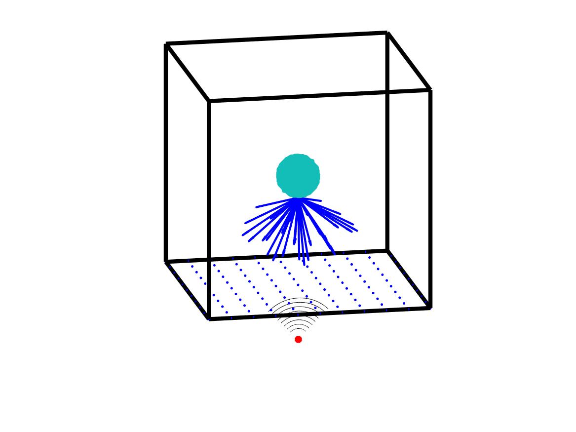
Figure 1: A diagram for the experiment that leads to Problem 5.1. The unknown object is located inside a box $\Omega$. An emitter (the red dot), located outside $\Omega$, emits the incident wave. The incident wave scatters when hitting the unknown object. The back scattering waves are represented by blue arrows and collected on an array of detectors, located on the part $\Gamma$ of $\partial\Omega$.

The forward problem corresponding to Problem 5.1 is the problem of computing the function $u(\mathbf{x},k)$, $(\mathbf{x},k)\in\Gamma\times[\underline{k},\overline{k}].$ To solve the forward problem, we first model the incident wave by the point source

$$u_{0}(\mathbf{x},k)=\frac{\exp(\mathrm{i}k|\mathbf{x}-\mathbf{x}_{0}|)}{4\pi|\mathbf{x}-\mathbf{x}_{0}|}\quad(\mathbf{x},k)\in\mathbb{R}^{3}\times[\underline{k},\overline{k}].$$ (5.5)

It is well-known that

$$\Delta u_{0}(\mathbf{x},k)+k^{2}u_{0}(\mathbf{x},k)=-\delta(\mathbf{x}-\mathbf{x}_{0})\quad\mathbf{x}\in\mathbb{R}^{3},k\in[\underline{k},\overline{k}].$$ (5.6)

Let

$$u_{\mathrm{sc}}(\mathbf{x},k)=u(\mathbf{x},k)-u_{0}(\mathbf{x},k)\quad\mathbf{x}\in\mathbb{R}^{3},k\in[\underline{k},\overline{k}]$$ (5.7)

denote the scattering wave. It follows from (5.7) that $u(\mathbf{x},k)$ is the sum of the scattering wave and the incident wave. We call the function $u(\mathbf{x},k)$ the total wave. Subtracting the differential equation in (5.2) from (5.6), we obtain

$$\Delta u_{\mathrm{sc}}(\mathbf{x},k)+k^{2}u_{\mathrm{sc}}(\mathbf{x},k)=-k^{2}(c(\mathbf{x})-1)u(\mathbf{x},k)\quad\mathbf{x}\in\mathbb{R}^{3},k\in[\underline{k},\overline{k}].$$

Hence, see [6, Chapter 8],

$$u_{\mathrm{sc}}(\mathbf{x},k)=k^{2}\int_{\mathbb{R}^{3}}\frac{\exp(\mathrm{i}k|\mathbf{x}-\xi|)}{4\pi|\mathbf{x}-\xi|}(c(\xi)-1)u(\xi,k)d\xi\quad\mathbf{x}\in\mathbb{R}^{3},k\in[\underline{k},\overline{k}].$$ (5.8)

Combining (5.7) and (5.8), we arrive at the Lippmann-Schwinger equation

$$u(\mathbf{x},k)=u_{0}(\mathbf{x},k)+k^{2}\int_{\mathbb{R}^{3}}\frac{\exp(\mathrm{i}k|\mathbf{x}-\xi|)}{4\pi|\mathbf{x}-\xi|}(c(\xi)-1)u(\xi,k)d\xi$$ (5.9)

for all $\mathbf{x}\in\mathbb{R}^{3},k\in[\underline{k},\overline{k}].$ We solve the integral equation (5.9) by the method in [25, 26]. In order to solve the inverse problem, we need to impose the following condition.

Assumption 2

The total wave $u(\mathbf{x},k)$ is nonzero for all $\mathbf{x}\in\Omega$ and $k\in[\underline{k},\overline{k}].$

We provide here an example when Assumption 2 holds true. In this example, we assume that $c$ is in the class $C^{15}(\mathbb{R}^{3})$. Consider the Riemannian metric generated by $c$

$$d\tau=\sqrt{c(\mathbf{x})}d\mathbf{x},\quad|d\mathbf{x}|=\sqrt{dx_{1}^{2}+dx_{2}^{2}+dx_{3}^{2}}.$$ (5.10)

Assume that for each point $\mathbf{x}\in\mathbb{R}^{3}$, the geodesic line with respect to the Riemannian metric defined (5.10) connecting $\mathbf{x}_{0}$ and $\mathbf{x}$ is unique, where $\mathbf{x}_{0}$ is the location of the emitter that emits the point source. Then, it was shown in [21] that

$$u(\mathbf{x},k)=A(\mathbf{x})e^{\mathrm{i}k\tau(\mathbf{x})}+O\Big{(}\frac{1}{k}\Big{)}\quad\mbox{as }k\to\infty$$ (5.11)

for $\mathbf{x}\in\Omega$ where $A$ is a function taking positive value and $\tau$ is the travel time of the wave from $\mathbf{x}_{0}$ to $\mathbf{x}$. Hence, Assumption 2 holds true when the wave number $k$ is sufficiently large. In the next section, we derive a system of nonlinear partial differential equations. Solution of this system directly yields the solution to Problem 5.1.

6 A method to solve Problem 5.1

Recall that $u=u(\mathbf{x},k)$, $\mathbf{x}\in\Omega$, $k\in[\underline{k},\overline{k}]$ is the solution to (5.2). Assume that Assumption 2 holds true. Define

$$v(\mathbf{x},k)=\frac{1}{k^{2}}\log\frac{u(\mathbf{x},k)}{u_{0}(\mathbf{x},k)}\quad\mbox{for all }\mathbf{x}\in\Omega,k\in[\underline{k},\overline{k}].$$ (6.1)

Although $u/u_{0}$ takes complex values, the function $v$ can be defined. Employing (5.11) and assuming that both $\underline{k}$ and $\overline{k}$ are large, we define the function $v$ as

$$v({\bf x},k) =\frac{1}{k^{2}}\big{[}\log u({\bf x},k)-\log u_{0}({\bf x},k)\big{]}$$

$$=\frac{1}{k^{2}}\Big{[}\ln A({\bf x})-\ln\frac{1}{4\pi|{\bf x}-{\bf x}_{0}|}+{\rm i}k(\tau({\bf x})-|{\bf x}-{\bf x}_{0}|)+O(1/k)\Big{]}$$

for all ${\bf x}\in\Omega,k\in[\underline{k},\overline{k}].$ We now derive a differential equation for the function $v$. It follows from (6.1) that

$$\nabla v(\mathbf{x},k)=\frac{1}{k^{2}}\Big{(}\frac{\nabla u(\mathbf{x},k)}{u(\mathbf{x},k)}-\frac{\nabla u_{0}(\mathbf{x},k)}{u_{0}(\mathbf{x},k)}\Big{)}\quad\mbox{for all }\mathbf{x}\in\Omega,k\in[\underline{k},\overline{k}].$$ (6.2)

Taking the divergence of (6.2) gives

$$\Delta v(\mathbf{x},k)=\frac{1}{k^{2}}\Big{(}\frac{\Delta u(\mathbf{x},k)}{u(\mathbf{x},k)}-\Big{(}\frac{\nabla u(\mathbf{x},k)}{u(\mathbf{x},k)}\Big{)}^{2}-\frac{\Delta u_{0}(\mathbf{x},k)}{u_{0}(\mathbf{x},k)}+\Big{(}\frac{\nabla u_{0}(\mathbf{x},k)}{u_{0}(\mathbf{x},k)}\Big{)}^{2}\Big{)}$$ (6.3)

for all $\mathbf{x}\in\Omega$, $k\in[\underline{k},\overline{k}]$. Since $u(\mathbf{x},k)$ satisfies the differential equation in (5.2) and $u_{0}(\mathbf{x},k)$ satisfies the differential equation in (5.2) with $c(\mathbf{x})$ replaced by $1$, we have

$$\frac{\Delta u(\mathbf{x},k)}{u(\mathbf{x},k)}=-k^{2}c(\mathbf{x})\quad\mbox{and}\quad\frac{\Delta u_{0}(\mathbf{x},k)}{u_{0}(\mathbf{x},k)}=-k^{2}$$ (6.4)

for all $\mathbf{x}\in\Omega$, $k\in[\underline{k},\overline{k}]$. It follows from (6.2), (6.3) and (6.4) that

$$\Delta v(\mathbf{x},k) =\frac{1}{k^{2}}\Big{[}-k^{2}(c(\mathbf{x})-1)-\Big{(}k^{2}\nabla v(\mathbf{x},k)+\frac{\nabla u_{0}(\mathbf{x},k)}{u_{0}(\mathbf{x},k)}\Big{)}^{2}+\Big{(}\frac{\nabla u_{0}(\mathbf{x},k)}{u_{0}(\mathbf{x},k)}\Big{)}^{2}\Big{]}$$

$$=-(c(\mathbf{x})-1)-k^{2}(\nabla v(\mathbf{x},k))^{2}-\frac{2\nabla v(\mathbf{x},k)\cdot\nabla u_{0}(\mathbf{x},k)}{u_{0}(\mathbf{x},k)}$$

for all $\mathbf{x}\in\Omega$, $k\in[\underline{k},\overline{k}]$. We obtain

$$\Delta v(\mathbf{x},k)+k^{2}(\nabla v(\mathbf{x},k))^{2}+\frac{2\nabla v(\mathbf{x},k)\cdot\nabla u_{0}(\mathbf{x},k)}{u_{0}(\mathbf{x},k)}=-c(\mathbf{x})+1$$ (6.5)

for all $\mathbf{x}\in\Omega$, $k\in[\underline{k},\overline{k}]$. Differentiate (6.5) with respect to $k$. We have

$$\Delta\partial_{k}v(\mathbf{x},k)+2k^{2}\nabla v(\mathbf{x},k)\cdot\nabla\partial_{k}v(\mathbf{x},k)+2k(\nabla v(\mathbf{x},k))^{2}\\ +2\nabla\partial_{k}v(\mathbf{x},k)\cdot\frac{\nabla u_{0}(\mathbf{x},k)}{u_{0}(\mathbf{x},k)}+2\nabla v(\mathbf{x},k)\partial_{k}\frac{\nabla u_{0}(\mathbf{x},k)}{u_{0}(\mathbf{x},k)}=0$$ (6.6)

for all $\mathbf{x}\in\Omega$, $k\in[\underline{k},\overline{k}]$.

Let $\{\Psi_{m}\}_{m\geq 1}$ be the orthonormal basis of $L^{2}(\Omega)$ defined in [15]. This basis is constructed as follows. For each $m\geq 1,$ define the function $\phi_{m}(k)=k^{m-1}e^{k-(\overline{k}+\underline{k})/2}$ for all $k\in[\underline{k},\overline{k}].$ It is clear that the set $\{\phi_{m}\}_{m\geq 1}$ is complete in $[\underline{k},\overline{k}].$ We then apply the Gram-Schmidt orthonormalization process to this set to obtain the basis $\{\Psi_{m}\}_{m\geq 1}$.

We derive an approximation model for the solution $v$ to (6.6) as follows. For each $\mathbf{x}\in\Omega$ and $k\in[\underline{k},\overline{k}],$ we write

$$v(\mathbf{x},k)=\sum_{i=1}^{\infty}v_{i}(\mathbf{x})\Psi_{i}(k)\simeq\sum_{i=1}^{N}v_{i}(\mathbf{x})\Psi_{i}(k)$$ (6.7)

for some cut-off number $N$, determined later in section 7, where

$$v_{i}(\mathbf{x})=\int_{\underline{k}}^{\overline{k}}v(\mathbf{x},\kappa)\Psi_{i}(\kappa)d\kappa\quad i\in\{1,\dots,N\}.$$ (6.8)

In this approximation context,

$$v_{k}(\mathbf{x},k)=\sum_{i=1}^{N}v_{i}(\mathbf{x})\Psi_{i}^{\prime}(k)\quad\mbox{for all }\mathbf{x}\in\Omega,k\in[\underline{k},\overline{k}].$$ (6.9)

Plugging (6.7) and (6.9) into (6.6) gives

$$\sum_{i=1}^{N}\Delta v_{i}(\mathbf{x})\Psi_{i}^{\prime}(k)+2\sum_{i,j=1}^{N}\nabla v_{i}(\mathbf{x})\cdot\nabla v_{j}(\mathbf{x})\Big{(}k^{2}\Psi_{i}(k)\Psi_{j}^{\prime}(k)+k\Psi_{i}(k)\Psi_{j}(k)\Big{)}\\ +2\sum_{i=1}^{N}\nabla v_{i}(\mathbf{x})\cdot\Big{(}\Psi_{i}^{\prime}(k)\frac{\nabla u_{0}(\mathbf{x},k)}{u_{0}(\mathbf{x},k)}+\Psi_{i}(k)\partial_{k}\frac{\nabla u_{0}(\mathbf{x},k)}{u_{0}(\mathbf{x},k)}\Big{)}=0$$ (6.10)

for all $\mathbf{x}\in\Omega.$ For each $l\in\{1,\dots,N\},$ multiplying $\Psi_{l}(k)$ to both sides of (6.10), we have

$$\sum_{i=1}^{N}s_{li}\Delta v_{i}(\mathbf{x})+\sum_{i,j=1}^{N}a_{lij}\nabla v_{i}(\mathbf{x})\cdot\nabla v_{j}(\mathbf{x})+\sum_{i=1}^{N}B_{li}(\mathbf{x})\cdot\nabla v_{i}(\mathbf{x})=0$$ (6.11)

where

$$\left\{\begin{array}[]{l}s_{li}=\displaystyle\int_{\underline{k}}^{\overline{k}}\Psi_{i}^{\prime}(k)\Psi_{l}(k)dk,\\ a_{lij}=\displaystyle 2\int_{\underline{k}}^{\overline{k}}\Big{(}k^{2}\Psi_{i}(k)\Psi_{j}^{\prime}(k)+k\Psi_{i}(k)\Psi_{j}(k)\Big{)}\Psi_{l}(k)dk,\\ B_{li}(\mathbf{x})=\displaystyle 2\int_{\underline{k}}^{\overline{k}}\Big{(}\Psi_{i}^{\prime}(k)\frac{\nabla u_{0}(\mathbf{x},k)}{u_{0}(\mathbf{x},k)}+\Psi_{i}(k)\partial_{k}\frac{\nabla u_{0}(\mathbf{x},k)}{u_{0}(\mathbf{x},k)}\Big{)}\Psi_{l}(k)dk\end{array}\right.$$ (6.12)

for all $i,j,l\in\{1,\dots,N\}$ and $\mathbf{x}\in\Omega$.

We next compute the boundary information for $V$. For all $\mathbf{x}\in\Gamma$ and $k\in[\underline{k},\overline{k}]$, since $u(\mathbf{x},k)=f(\mathbf{x},k)$ where $f$ is the data for the inverse problem under consideration (see (5.4)), it follows from (6.1) that $v(\mathbf{x},k)=\frac{1}{k^{2}}\log\frac{f(\mathbf{x},k)}{u_{0}(\mathbf{x},k)}$. Hence, by (6.8), we have

$$v_{i}(\mathbf{x})=\int_{\underline{k}}^{\overline{k}}v(\mathbf{x},\kappa)\Psi_{i}(\kappa)d\kappa=\int_{\underline{k}}^{\overline{k}}\frac{1}{\kappa^{2}}\log\frac{f(\mathbf{x},\kappa)}{u_{0}(\mathbf{x},\kappa)}\Psi_{i}(\kappa)d\kappa\quad i\in\{1,\dots,N\}$$

for all $\mathbf{x}\in\Gamma.$ Since we only measure the wave $u$ on $\Gamma,$ we complement $v_{i}(\mathbf{x})=0$ for all $i\in\{1,\cdots,N\}$ and $\mathbf{x}\in\partial\Omega\setminus\Gamma.$ The boundary value of $V_{N}=(v_{1},v_{2},\dots,v_{N})^{\rm T}$ is given by

$$V_{N}({\bf x})=g_{1}(\mathbf{x})=\left\{\begin{array}[]{ll}\begin{array}[]{c}\Big{[}\displaystyle\int_{\underline{k}}^{\overline{k}}\frac{1}{\kappa^{2}}\log\frac{f(\mathbf{x},\kappa)}{u_{0}(\mathbf{x},\kappa)}\Psi_{i}(\kappa)d\kappa\Big{]}_{i=1}^{N}\end{array}&\mathbf{x}\in\Gamma,\\ 0&\mathbf{x}\in\partial{\Omega}\setminus\Gamma\end{array}\right.$$ (6.13)

On the other hand, by (6.8), for all $\mathbf{x}\in\Gamma$ and $k\in[\underline{k},\overline{k}]$,

$$\partial_{\nu}v(\mathbf{x},k)=\frac{1}{k^{2}}\Big{(}\frac{\partial_{\nu}u(\mathbf{x},k)}{u(\mathbf{x},k)}-\frac{\partial_{\nu}u_{0}(\mathbf{x},k)}{u_{0}(\mathbf{x},k)}\Big{)}=\frac{1}{k^{2}}\Big{(}\frac{g(\mathbf{x},k)}{f(\mathbf{x},k)}-\frac{\partial_{\nu}u_{0}(\mathbf{x},k)}{u_{0}(\mathbf{x},k)}\Big{)}.$$

Therefore, by (6.8),

$$\partial_{\nu}v_{i}(\mathbf{x}) =\int_{\underline{k}}^{\overline{k}}\partial_{\nu}v(\mathbf{x},\kappa)\Psi_{i}(\kappa)d\kappa$$

$$=\int_{\underline{k}}^{\overline{k}}\frac{1}{\kappa^{2}}\Big{(}\frac{g(\mathbf{x},\kappa)}{f(\mathbf{x},\kappa)}-\frac{\partial_{\nu}u_{0}(\mathbf{x},\kappa)}{u_{0}(\mathbf{x},\kappa)}\Big{)}\Psi_{i}(\kappa)d\kappa$$ (6.14)

for all $i\in\{1,\dots,N\}$ and $\mathbf{x}\in\Gamma.$ By setting

$$g_{0}(\mathbf{x})=\left[\int_{\underline{k}}^{\overline{k}}\frac{1}{\kappa^{2}}\Big{(}\frac{g(\mathbf{x},\kappa)}{f(\mathbf{x},\kappa)}-\frac{\partial_{\nu}u_{0}(\mathbf{x},\kappa)}{u_{0}(\mathbf{x},\kappa)}\Big{)}\Psi_{i}(\kappa)d\kappa\right]_{i=1}^{N},$$ (6.15)

we have

$$\partial_{\nu}V(\mathbf{x})=g_{0}(\mathbf{x})\quad\mbox{for all }\mathbf{x}\in\Gamma.$$ (6.16)

In summary, the vector $V_{N}=(v_{1},v_{2},\dots,v_{N})^{\rm T}$ satisfies a Cauchy like boundary value problem

$$\left\{\begin{array}[]{rcll}\displaystyle\sum_{i=1}^{N}s_{li}\Delta v_{i}(\mathbf{x})+\sum_{i,j=1}^{N}a_{lij}\nabla v_{i}(\mathbf{x})\cdot\nabla v_{j}(\mathbf{x})\\ \hskip 85.35826pt+\displaystyle\sum_{i=1}^{N}B_{li}(\mathbf{x})\cdot\nabla v_{i}(\mathbf{x})&=&0,&\quad{\bf x}\in\Omega,\\ V_{N}({\bf x})&=&g_{1}({\bf x})&\quad{\bf x}\in\partial\Omega,\\ \partial_{\nu}V_{N}({\bf x})&=&g_{0}({\bf x})&\quad{\bf x}\in\Gamma.\end{array}\right.$$ (6.17)

where $s_{ij}$, $a_{lij}$, $B_{li}$, $1\leq i,j,l\leq N$ are given in (6.12), $g_{1}$ and $g_{0}$, are respectively defined in (6.13) and (6.15).

Remark 5

Let $(\tilde{s}_{li})_{l,i=1}^{N}$ denote $S^{-1}$. Problem (6.17) can be rewritten as a particular form of (3.1) as

$$\left\{\begin{array}[]{rcll}\displaystyle\sum_{i=1}^{N}\Delta v_{i}(\mathbf{x})+\sum_{i,j=1}^{N}\tilde{s}_{li}a_{lij}\nabla v_{i}(\mathbf{x})\cdot\nabla v_{j}(\mathbf{x})\\ \hskip 85.35826pt+\displaystyle\sum_{i=1}^{N}\tilde{s}_{li}B_{li}(\mathbf{x})\cdot\nabla v_{i}(\mathbf{x})&=&0,&\quad{\bf x}\in\Omega,\\ V_{N}({\bf x})&=&g_{1}({\bf x})&\quad{\bf x}\in\partial\Omega,\\ \partial_{\nu}V_{N}({\bf x})&=&g_{0}({\bf x})&\quad{\bf x}\in\Gamma.\end{array}\right.$$

However, we numerically observe that solving (6.17) provides better numerical solutions.

Let $\mu_{\lambda}(x,y,z)=e^{\lambda(z+r)^{2}}$ for a number $r>1$ be a Carleman weight function. We refer the reader to [10, Theorem 3.1] for the proof of Carleman estimate (3.9) with this Carleman weight function in 3D. Thus, we can find the solution to the system of quasi-linear equations (6.17) by the convexification method, see Algorithm 1.

7 Numerical tests

In this section, we numerically study Problem 3.1 and Problem 5.1.

7.1 Numerical study for Problem 3.1

We present an example in which we apply convexification method to compute the solution to problem of the form (3.1). For simplicity, we consider the case $n=2$ and the computational domain $\Omega$ is chosen to be $(-1,1)^{2}$. We choose the set $\Gamma$ to be $\{(x,y=-1):|x|\leq 1\}\subset\partial\Omega$, on which we impose the Neumann boundary condition for the solution $v$. We numerically test the convexification method in the finite difference scheme. That means we compute the values of the solution on the grid

$$\mathcal{G}=\big{\{}(x_{i}=-1+(i-1)d_{{\bf x}},y_{j}=-1+(j-1)d_{{\bf x}}):1\leq i,j\leq N_{{\bf x}}\big{\}}$$

where $d_{\bf x}=\frac{2}{N_{{\bf x}}-1}$ and $N_{{\bf x}}$ is an integer. In our numerical study, $N_{{\bf x}}=41.$

In computation, we use the Carleman weight function $e^{-\lambda(R+1.5)^{2}}e^{\lambda(y-1.5)^{2}}$ where $\lambda=1.1$. This Carleman weight function is the 2D version of the one used in Section 7.2. The regularization term is chosen to be $\epsilon=10^{-6}.$ The details in implementation including the discretizing the cost functional $J_{\epsilon,\lambda}$ and the choice of the initial guess are similar to the ones in Section 7.2. We do not present in details here. To illustrate the efficiency of Algorithm 1, we compute solution to (3.1) when the nonlineariry $G$ is given by

$$G({\bf x},s,p)=-\sqrt{|p|^{2}+1}-\sin\left(x+\pi\,\left(y-0.5\right)^{2}\right)+2\,\pi\,\cos\left(x+\pi\,\left(y-0.5\right)^{2}\right)\\ -4\,{\pi}^{2}\left(y-0.5\right)^{2}\sin\left(x+\pi\,\left(y-0.5\right)^{2}\right)+\Big{[}\left(1+\cos\left(x+\pi\,\left(y-0.5\right)^{2}\right)\right)^{2}\\ +4\,{\pi}^{2}\left(y-0.5\right)^{2}\left(\cos\left(x+\pi\,\left(y-0.5\right)^{2}\right)\right)^{2}+1\Big{]}^{1/2}$$ (7.1)

for all ${\bf x}=(x,y)\in\Omega$, $s\in\mathbb{R}$ and $p\in\mathbb{R}^{d}$. The exact boundary data are given by

$$\left\{\begin{array}[]{ll}g_{1}^{*}(x,y)=x+\sin\big{(}x+\pi(y-0.5)^{2}\big{)}&(x,y)\in\partial\Omega,\\ g_{0}^{*}(x,y)=-2\pi(y-0.5)\cos\big{(}x+\pi(y-0.5)^{2}\big{)}&(x,y)\in\Gamma.\end{array}\right.$$ (7.2)

We add noise into the boundary data by the following formulas

$$g_{1}=g_{1}^{*}(1+\delta{\rm rand})\quad\mbox{and }\quad g_{0}=g_{0}^{*}(1+\delta{\rm rand})$$

where rand is a function taking uniformly distributed random numbers in the range $[-1,1].$ The noise level $\delta$ is set to be $5\%$, $10\%$ and $20\%$. The exact solution to (3.1) in this test is $v^{*}(x,y)=x+\sin\big{(}x+\pi(y-0.5)^{2}\big{)}$ for all ${\bf x}=(x,y)\in\Omega.$ The error in computation is given in Table 1.

$\delta$	relative error $\frac{\|v^{*}-v^{\rm comp}\|_{L^{\infty}(\Omega)}}{\|v^{*}\|_{L^{\infty}(\Omega)}}$
5%	4.14%
10%	9.21%
20%	19.40%

Table 1: The relative error in our computation agaist the noise level $\delta$ contained in the boundary data.

The graphs of the exact solution $v^{*}$, computed solution $v^{\rm comp}$ and their relative differences $\frac{|v^{*}-v^{\rm comp}|}{\|v^{*}\|_{L^{\infty}(\Omega)}},$ when $\delta=5\%,$ $10\%$ and $20\%$ are displayed in Figure 2.

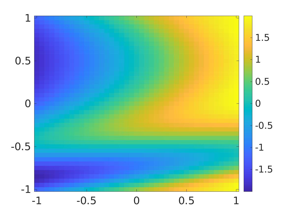
(a) The function $v^{*}$

(b) The function $v^{\rm comp}$. $\delta=5\%$.

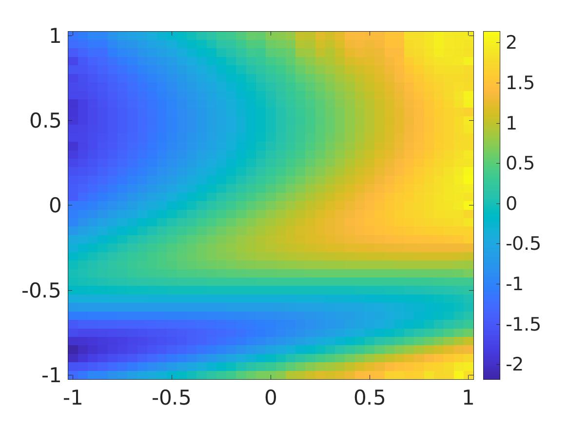
(c) The function $v^{\rm comp}$. $\delta=10\%$.

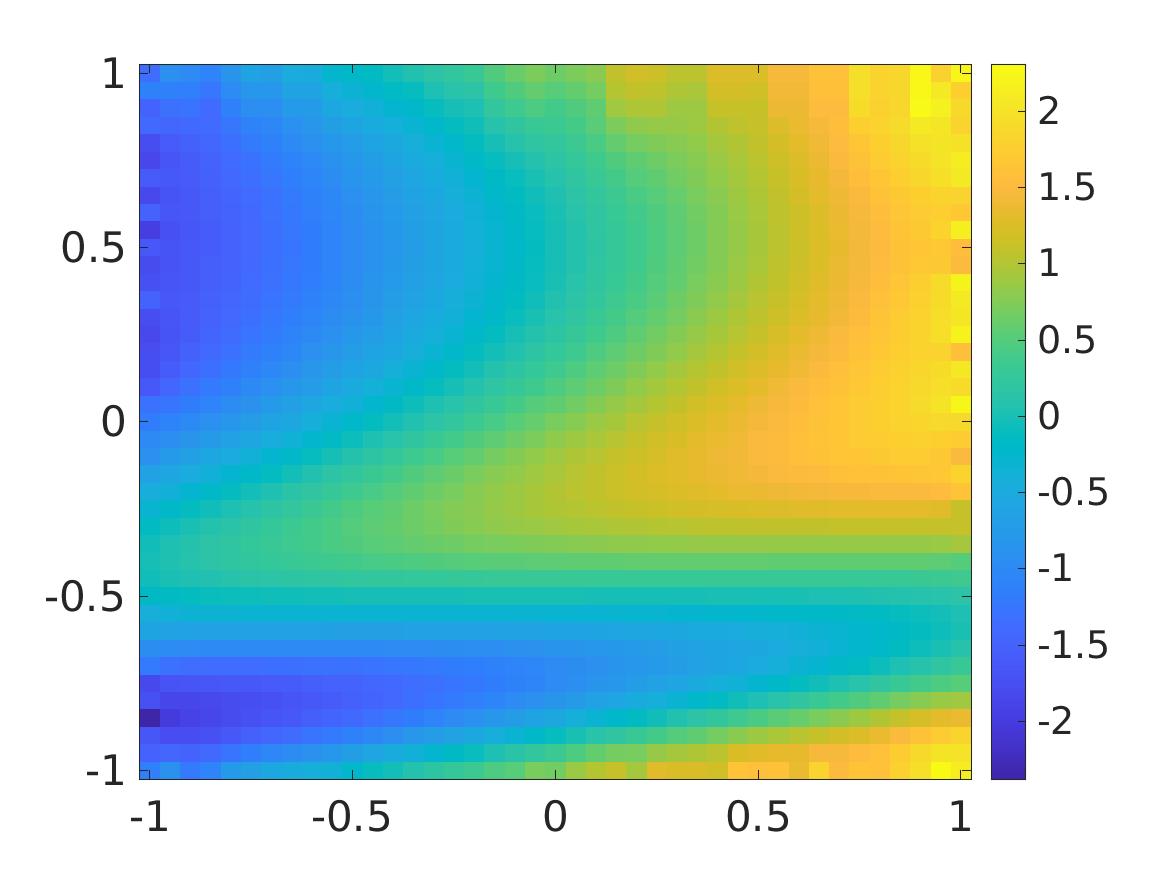
(d) The function $v^{\rm comp}$. $\delta=20\%$.

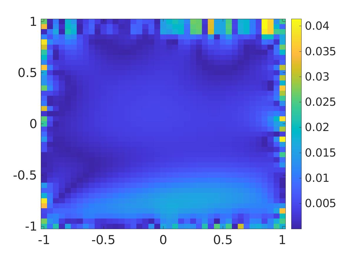
(e) The relative difference $\frac{|v^{*}-v^{\rm comp}|}{\|v^{*}\|_{L^{\infty}(\Omega)}}$. $\delta=5\%$

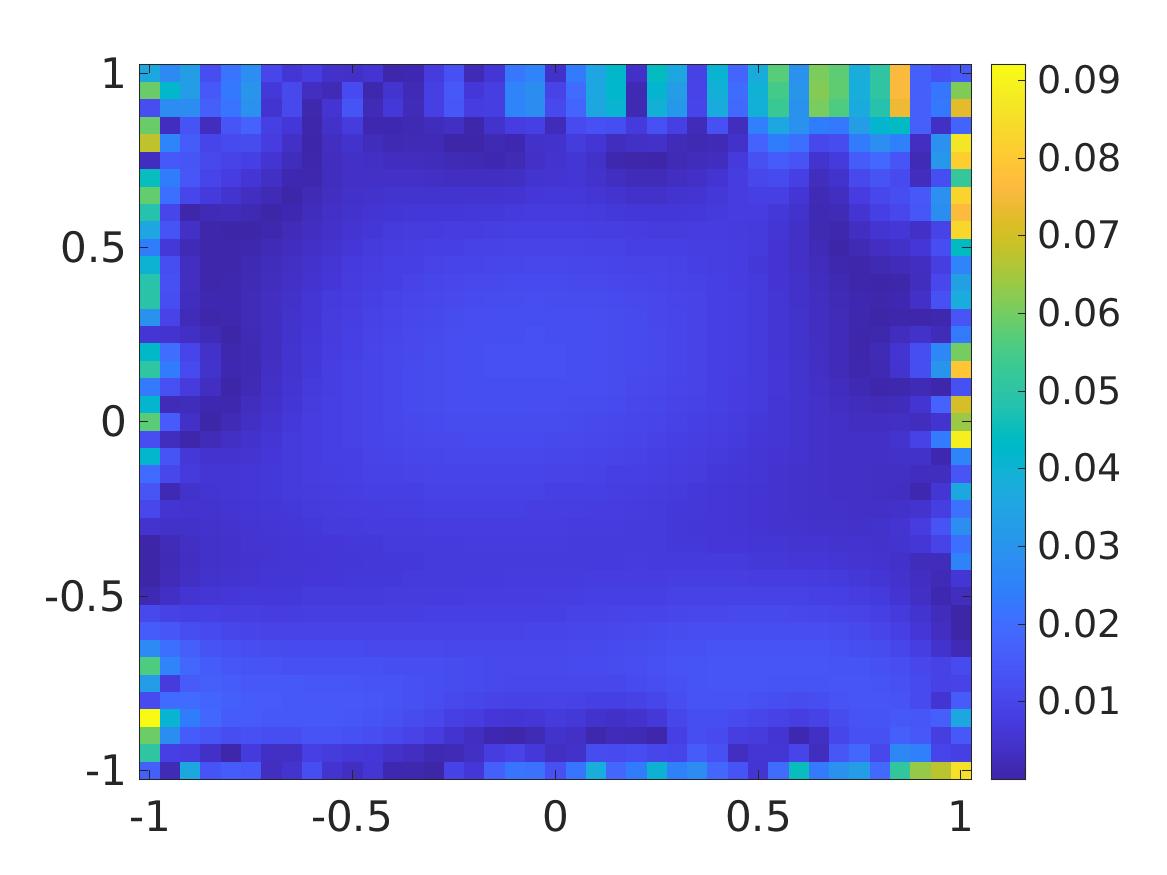
(f) The relative difference $\frac{|v^{*}-v^{\rm comp}|}{\|v^{*}\|_{L^{\infty}(\Omega)}}$. $\delta=10\%$

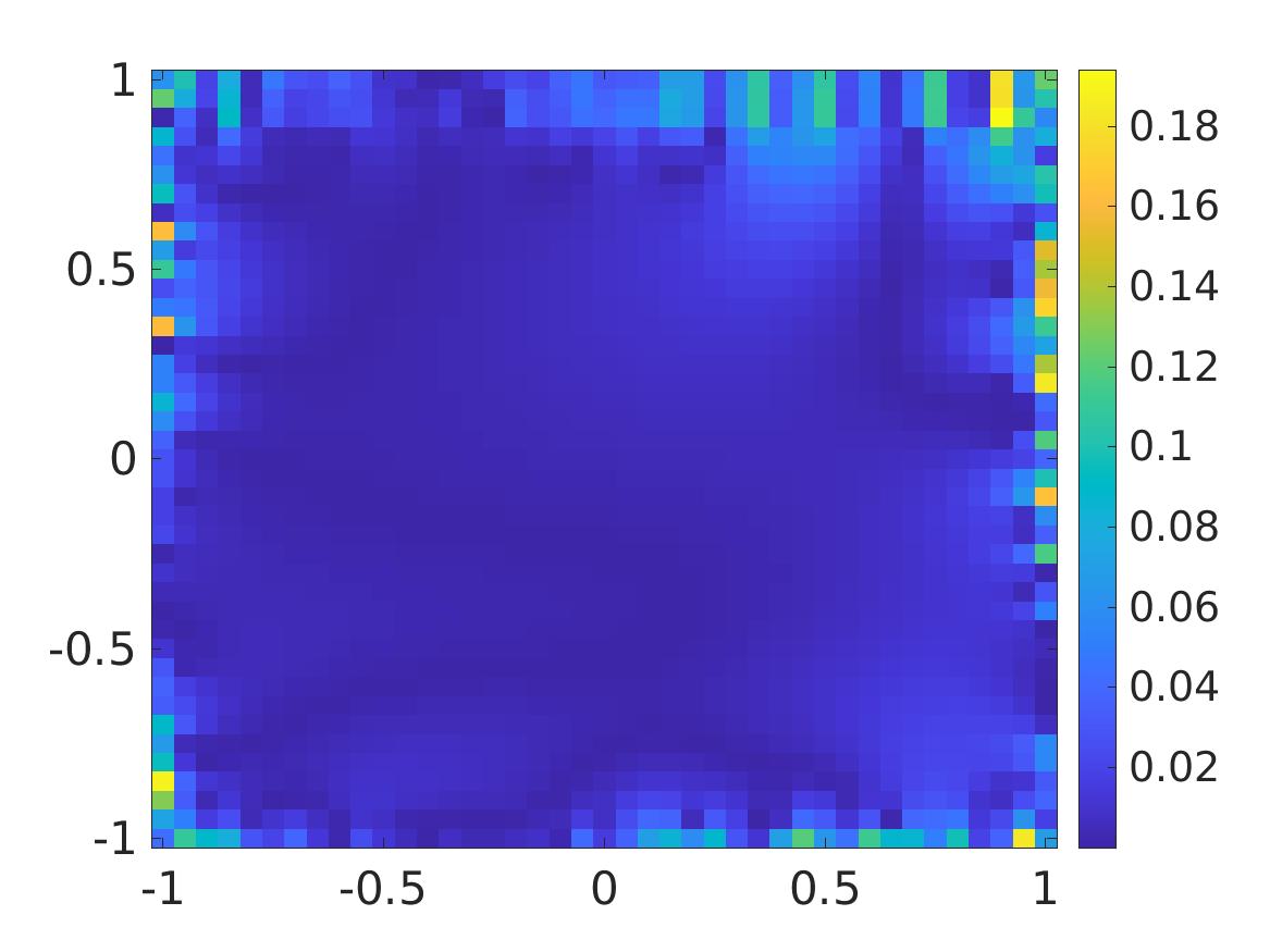
(g) The relative difference $\frac{|v^{*}-v^{\rm comp}|}{\|v^{*}\|_{L^{\infty}(\Omega)}}$. $\delta=20\%$

Figure 2: Solutions to (3.1) when $G$ and $f^{*}$ and $g^{*}$ are given in (7.1) and (7.2) respectively.

It is evident from Table 1 and Figure 2 that the convexification method delivers reliable solutions to quasi-linear elliptic equations. The errors in computation are compatible with the noise level and they occur on $\partial\Omega$ where the noise takes place.

7.2 Numerical study for Problem 5.1

In this section, we present some numerical solutions to Problem 5.1. The numerical examples we present in this section illustrate the efficiency of the gradient descent method for the convexification described in section 4. Especially, we will show that the presence of the Carleman weight function in the objective function is crucial. That means, without involving the Carleman estimate, the descent gradient method does not deliver good numerical solutions to the problem of minimizing our nonconvex objective functional.

7.2.1 The forward problem

The experimental setting for Problem 5.1 is as follows. Let $R=1$ and $\Omega=(-R,R)^{3}$. The source location is placed at $(0,0,-4)$. The interval of wavenumbers is $[\pi,2\pi]$, which correspond to the interval of wavelengths $[0.5,1].$ In order to generate the simulated data, we use the finite difference method in which we decompose $\Omega$ as the uniform partition with grid points

$$\mathcal{G}=\{(x_{i}=-R+(i-1)h,y_{j}=-R+(j-1)h,z_{l}=-R+(l-1)h):\\ 1\leq i,j,k\leq N_{\mathbf{x}}\}$$

where $N_{\mathbf{x}}=41$ and $h=2R/(N_{\mathbf{x}}-1)$. We also split the interval of wavenumbers to the uniform partition

$$\mathcal{K}=\{k_{1}=\underline{k},k_{2},\dots,k_{N_{k}}=\overline{k}\}$$

where $k_{i}=\underline{k}+(i-1)(\overline{k}-\underline{k})/(N_{k}-1)$ and $N_{k}=121.$ The forward problem is solved via solving the Lippmann-Schwinger equation (5.9) by the method in [25, 26]. Denote by $u^{*}(\mathbf{x},k)$, $\mathbf{x}\in\mathcal{G}$, $k\in\mathcal{K}$ the obtained solution. The noisy data for Problem 5.1 is given by

$$f(\mathbf{x},k)=u(\mathbf{x},k)(1+\delta\mathrm{rand})\quad g(\mathbf{x},k)=-\partial_{z}u^{*}(\mathbf{x},k)(1+\delta\mathrm{rand})$$

for all $\mathbf{x}\in\Gamma\cap\mathcal{G}$ and $k\in\mathcal{K}$ where $\Gamma$ is the measurement site defined in (5.3), $\delta=10\%$ and $\mathrm{rand}$ is the function taking uniformly distributed random numbers in $[-1,1].$ The truncation number $N$ is $7$, which is chosen by a trial-error process.

7.2.2 The first approximation of the function $V$

The first step of our method is to compute a vector valued function that satisfies

$$\partial_{\nu}V_{0}|_{\Gamma}=g_{0}\quad\mbox{and}\quad V_{0}|_{\partial\Omega}=g_{1}.$$ (7.3)

This vector valued function $V_{0}$ is used in the change of variable $U=V-V_{0}$ as in (3.3). Moreover, to guarantee the fast convergence, we will find $V_{0}$ such that it is close to the solution $V$. We call this function $V_{0}$ the initial solution.

Since our target is to solve the nonlinear system (6.17), it is natural to find $V_{0}=(v^{0}_{1},v^{0}_{2},\dots,v^{0}_{N})$ as the solution to a linear system obtained by removing from (6.17) the nonlinear term, which is

$$\left\{\begin{array}[]{rcll}\displaystyle\sum_{i=1}^{N}s_{li}\Delta v_{i}^{0}(\mathbf{x})\displaystyle+\sum_{i=1}^{N}B_{li}(\mathbf{x})\cdot\nabla v_{i}^{0}(\mathbf{x})&=&0,&\quad{\bf x}\in\Omega,\\ V_{0}({\bf x})&=&g_{1}({\bf x})&\quad{\bf x}\in\partial\Omega,\\ \partial_{\nu}V_{0}({\bf x})&=&g_{0}({\bf x})&\quad{\bf x}\in\Gamma.\end{array}\right.$$ (7.4)

Since (7.4) is a system of linear partial differential equations, we can solve it directly by the quasi-reversibility method involving a Carleman weight function in the finite difference scheme. That means, we minimize the following functional

$$W\mapsto\int_{\Omega}\mu_{\lambda}^{2}\Big{|}\sum_{i=1}^{N}s_{li}\Delta w(\mathbf{x})+\sum_{i=1}^{N}B_{li}(\mathbf{x})\cdot\nabla W(\mathbf{x})\Big{|}^{2}+\epsilon\|W\|_{H^{2}(\Omega)}^{2}$$ (7.5)

where $W=(w_{1},w_{2},\dots,w_{N})$ is subject to the boundary conditions $W|_{\partial\Omega}=g_{1}$ and $\partial_{\nu}W|_{\Gamma}=g_{0}$. In (7.5) and also in this section, the used Carleman weight function is $\mu_{\lambda}=e^{-\lambda(R+r)^{2}}e^{\lambda(z-r)^{2}}$ where $\lambda=1.1$ and $r=1.5$ and the regularization parameter $\epsilon=10^{-6}$. Even though in theory, the value of $\lambda$ is large. However, we have discovered computationally that a reasonable value $\lambda=1.1$ works well. So, we use this $\lambda$. These observations coincide with those of our previous works on the numerical studies of the convexification [19, 10]. This Carleman weight function is used for all numerical tests in this section.

We refer the reader to [24, 28] for details in the implementation of the quasi-reversibility method to solve a system of linear partial differential equations with Cauchy boundary data.

7.2.3 The minimizing sequence

For the simplification in implementation, we skip the step of changing the variable $U=V-V_{0}$ as in (3.3). Let $U=V-V_{0}$ where $V_{0}=(v_{1}^{0},\dots,v_{N}^{0})$ is the vector valued function found in section 7.2.2. Then, due to (6.11), we set the cost functional as

$$J(U)=\sum_{l=1}^{N}\int_{\Omega}\mu_{\lambda}^{2}\Big{|}\sum_{i=1}^{N}s_{li}\Delta v_{i}-\sum_{i,j=1}^{N}a_{lij}\nabla v_{i}\cdot\nabla v_{j}-\sum_{i=1}^{N}B_{li}\nabla v_{i}\Big{)}\Big{|}^{2}d\mathbf{x}+\epsilon\|V\|^{2}_{H^{2}(\Omega)^{N}}.$$

The finite difference version of $J$ is

$$J(V)=h^{3}\sum_{\mathfrak{i,j,l=1}}^{N_{\mathbf{x}}}\sum_{l=1}^{N}\mu_{\lambda}^{2}(x_{\mathfrak{i}},y_{\mathfrak{j}},z_{\mathfrak{l}})\Big{|}\sum_{i=1}^{N}s_{li}\Delta v_{i}(x_{\mathfrak{i}},y_{\mathfrak{j}},z_{\mathfrak{l}})\\ -\sum_{i,j=1}^{N}a_{lij}\nabla v_{i}(x_{\mathfrak{i}},y_{\mathfrak{j}},z_{\mathfrak{l}})\cdot\nabla v_{j}(x_{\mathfrak{i}},y_{\mathfrak{j}},z_{\mathfrak{l}})-\sum_{i=1}^{N}B_{li}(x_{\mathfrak{i}},y_{\mathfrak{j}},z_{\mathfrak{l}})\nabla v_{i}(x_{\mathfrak{i}},y_{\mathfrak{j}},z_{\mathfrak{l}})\Big{|}^{2}d\mathbf{x}\\ +\epsilon h^{3}\sum_{\mathfrak{i,j,l=1}}^{N_{\mathbf{x}}}\sum_{l=1}^{N}\Big{(}|v_{l}(x_{\mathfrak{i}},y_{\mathfrak{j}},z_{\mathfrak{l}})|^{2}+|\nabla v_{l}(x_{\mathfrak{i}},y_{\mathfrak{j}},z_{\mathfrak{l}})|^{2}+|\Delta v_{l}(x_{\mathfrak{i}},y_{\mathfrak{j}},z_{\mathfrak{l}})|^{2}\Big{)}.$$ (7.6)

Remark 6

In our computation, $\epsilon=10^{-6}$ for all tests. Also, in (7.6), the regularity term is set to be $\epsilon\|U\|_{H^{2}(\Omega)^{N}}$ instead of $H^{p}(\Omega)^{N}$. We observe numerically that using the norm $\|U\|_{H^{2}(\Omega)^{N}}$ already provides satisfactory numerical solutions. So, it is not necessary for us to choose norm in $H^{p}(\Omega)^{N}$. This observation significantly reduces the expensive efforts in implementation.

We now mention that to speed up the minimization procedure, we need to compute the gradient $DJ_{1}$ of the discrete functional $J_{1}$ in (7.6) above. Having the expression for the gradient via an explicit formula significantly reduces the computational time. We have derived such a formula using the technique of Kronecker deltas, which has been outlined in [23]. For brevity we do not provide this formula here.

7.2.4 Numerical examples

We perform three (3) tests.

Test 1. We first consider the case of detecting one target with high dielectric constant. The dielectric constant of the medium is given by

$$c_{\mathrm{true}}=\left\{\begin{array}[]{ll}5&\mbox{if }0.6x^{2}+y^{2}+(z+0.7)^{2}\leq 0.2^{2},\\ 1&\mbox{otherwise}.\end{array}\right.$$

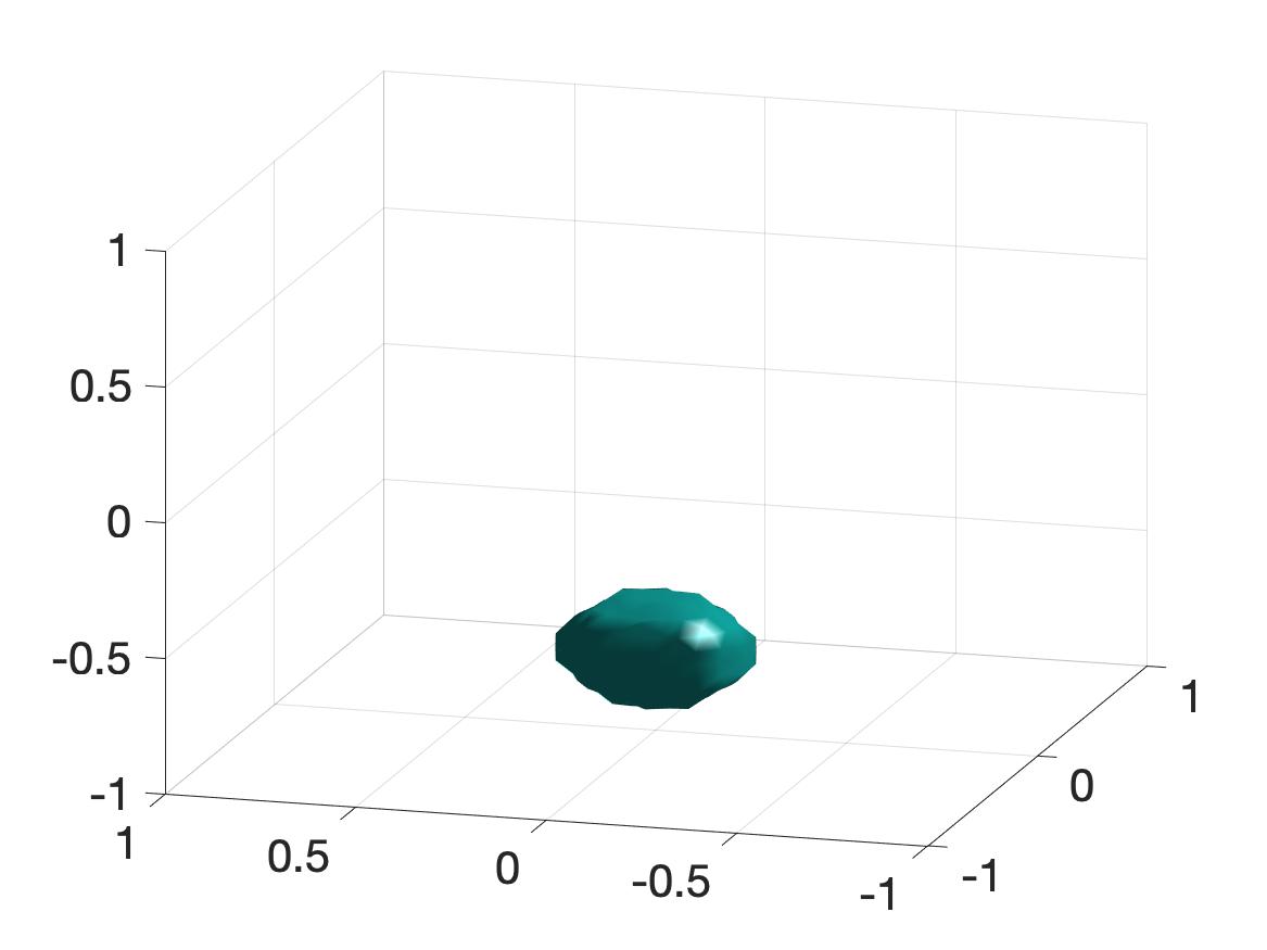
(a) The true 3D image

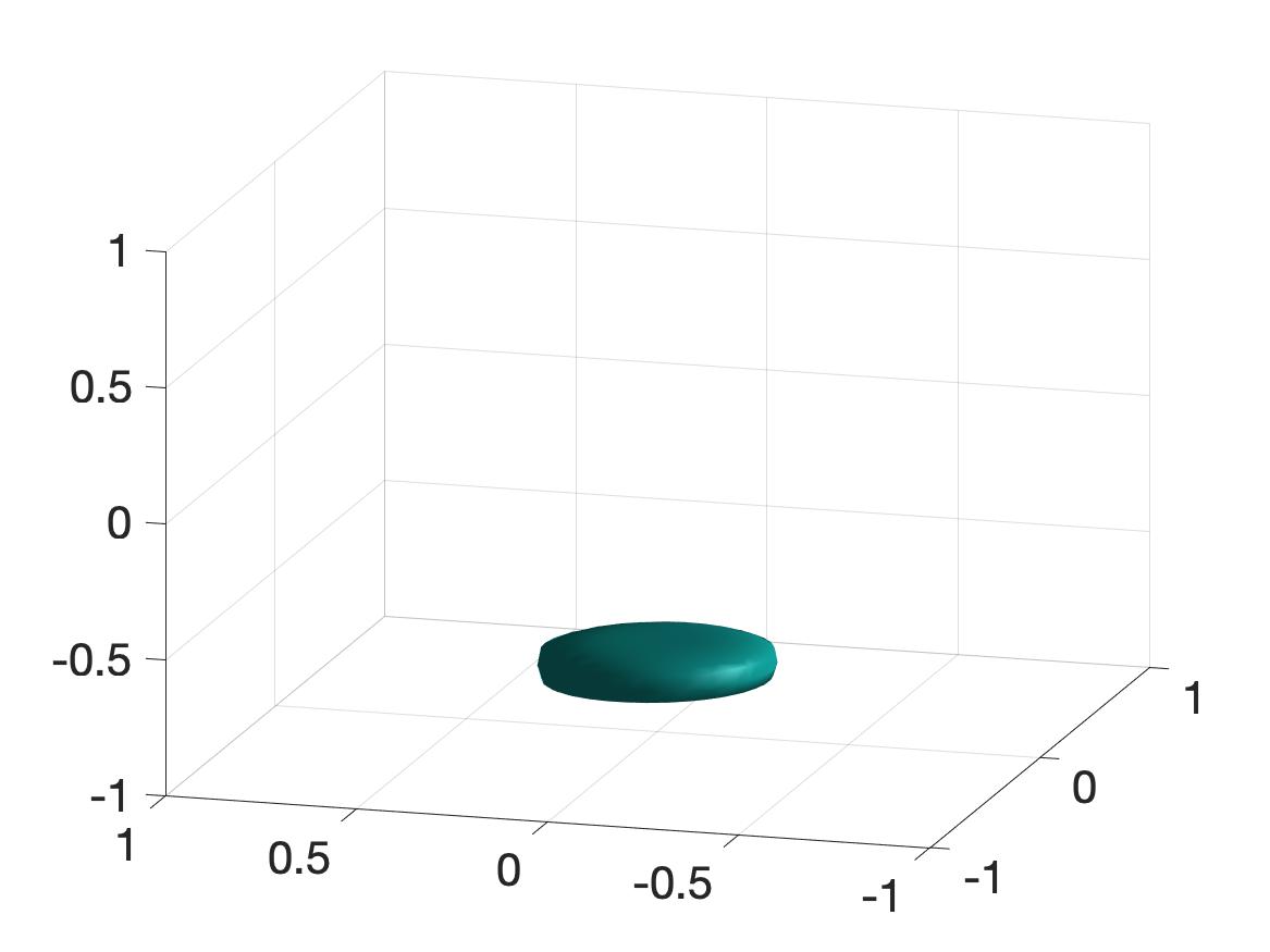
(b) The reconstructed 3D image

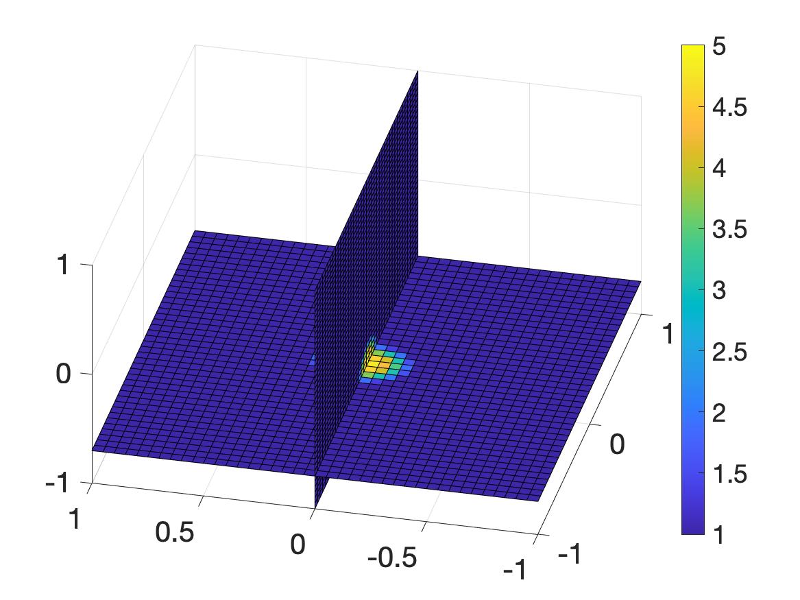
(c) The cross sections $\{z=-0.7\}$ and $\{y=0\}$ of $c_{\rm true}$

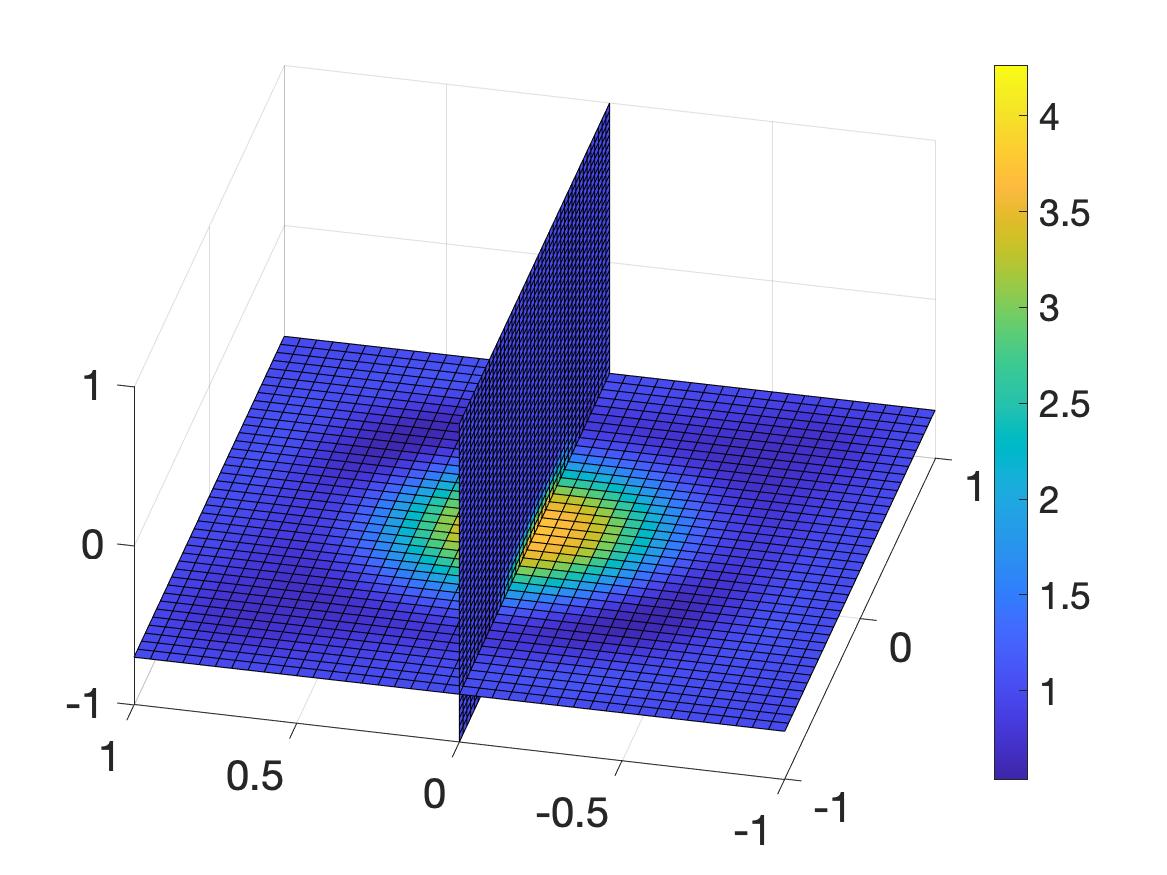
(d) The cross sections $\{z=-0.7\}$ and $\{y=0\}$ of $c_{\rm comp}$

Figure 3: Test 1. The function $c_{\mathrm{true}}$ and its reconstruction $c_{\mathrm{comp}}$ from noisy data with noise level of $10\%.$

The true and computed dielectric constants are displayed in Figure 3. It is obvious that the location of the target is detected accurately. The reconstructed shape is somewhat acceptable. The computed maximal value of the dielectric constant is $4.26$ (relative error 14.8%)).

Test 2. We test our method when the true dielectric constant is given by

$$c_{\mathrm{true}}=\left\{\begin{array}[]{ll}3&\mbox{if }0.35^{2}\leq x^{2}+y^{2}\leq 0.5^{2}\mbox{ and }-0.8\leq z\leq-0.65\\ 1&\mbox{otherwise}.\end{array}\right.$$

The shape of the dielectric constant is a ring.

(a) The true 3D image of the ring

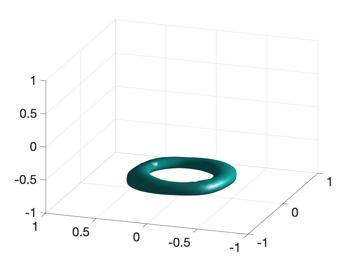
(b) The reconstructed 3D image of the ring

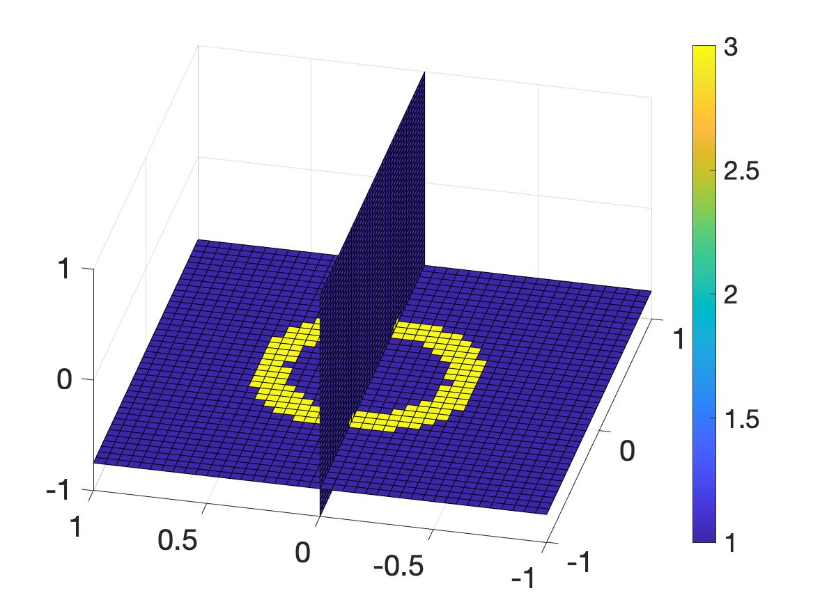
(c) The cross sections $\{z=-0.7\}$ and $\{y=0\}$ of $c_{\rm true}$

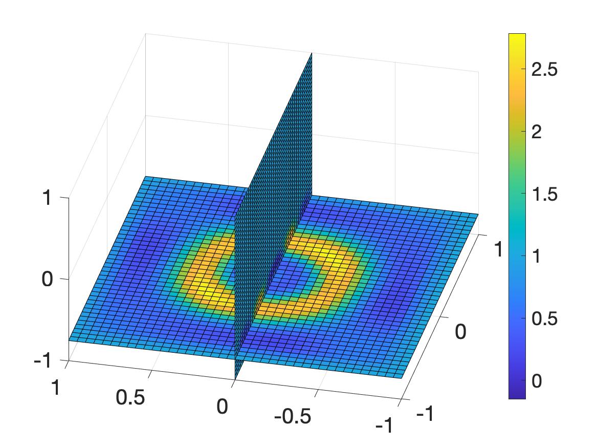
(d) The cross sections $\{z=-0.7\}$ and $\{y=0\}$ of $c_{\rm comp}$

Figure 4: Test 2. The function $c_{\mathrm{true}}$ and its reconstruction $c_{\mathrm{comp}}$ from noisy data with noise level of $10\%.$

The true and computed dielectric constants are displayed in Figure 4. It is an evident that the dielectric constant is computed successfully. The “ring” shape is clearly detected. The computed maximal value of the dielectric constant is $2.7809$ (relative error 7.3%)).

We now consider the direct optimization without using the Carleman weight function. That means we apply the same procedure to compute the dielectric constant except taking $\lambda=0.$ The numerical result in Figure 5 show that without the Carleman weight function involving, we reconstruction is poor.

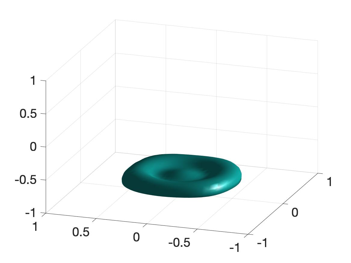
(a) The 3D image computed without using the convexification method

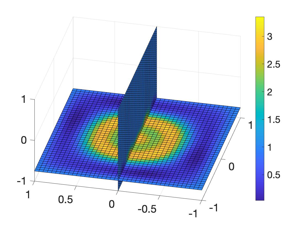
(b) The cross sections $\{z=-0.75\}$ and $\{y=0\}$ of $c_{\rm comp}$

Figure 5: Test 2. The function $c_{\mathrm{true}}$ and its reconstruction $c_{\mathrm{comp}}$ from noisy data with noise level of $10\%$ without using Carleman weight function. It is evident that in this case, the “ring” shape cannot be reconstructed well.

Test 3. We consider dielectric constant with a more complicate geometry. The graph of the dielectric constant is a letter $Y$ located on the plane $z=-.7$

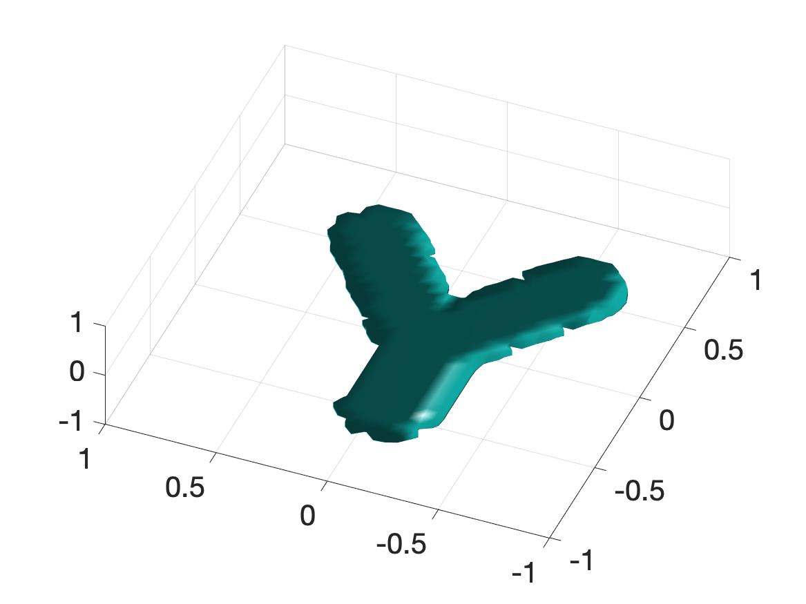
(a) The true 3D image of the letter $Y$

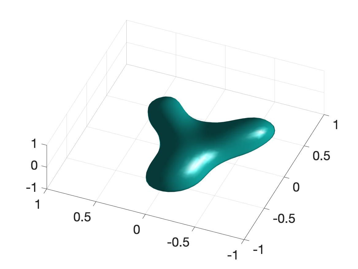
(b) The reconstructed 3D image of the letter $Y$

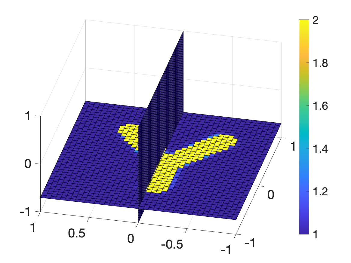
(c) The cross sections $\{z=-0.7\}$ and $\{y=0\}$ of $c_{\rm true}$

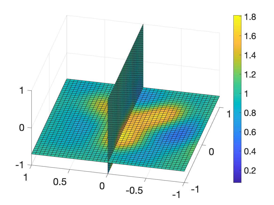
(d) The cross sections $\{z=-0.7\}$ and $\{y=0\}$ of $c_{\rm comp}$

Figure 6: Test 3. The function $c_{\mathrm{true}}$ and its reconstruction $c_{\mathrm{comp}}$ from noisy data with noise level of $10\%.$

The true and constructed dielectric constants are displayed in Figure 6. We observe that our method can detect the shape of the letter $Y$ clearly. Moreover, the reconstructed value of the dielectric constant is acceptable. The computed maximal value of the function $c$ is $1.8116$ (relative error 9.4%).

8 Concluding remarks

In the first part of this paper, we proved the convergence of the gradient descent method to find the minimizer of a functional which is strictly convex on a ball in a Hilbert space, rather than on the whole space. This is a new result, compared with previously obtained ones by our research team for the case of a more complicated gradient projection method. Then we used the convexification method and gradient descent method to solve a boundary value problem of quasi-linear PDE with both Dirichlet and Neumann data. We proved that this approach provides good numerical solutions as the noise tends to zero. In the second part of the paper, we applied the theoretical results of the first part to solve an inverse scattering problem. To solve this inverse problem, we derive an approximate mathematical model, which is the Cauchy problem for a coupled system of quasilinear elliptic partial differential equations. Then, we apply the convexification and the gradient descent method to solve this system. Numerical results for the inverse scattering problem demonstrate a good reconstruction quality.

References

- [1] O.M. Alifanov. Inverse heat conduction problems. Springer, New York, 1994.
- [2] O.M. Alifanov, A.E. Artukhin, and S.V. Rumyantcev. Extreme Methods for Solving Ill-Posed Problems with Applications to Inverse Heat Transfer Problems. Begell House, New York, 1995.
- [3] A. B. Bakushinskii, M. V. Klibanov, and N. A. Koshev. Carleman weight functions for a globally convergent numerical method for ill-posed Cauchy problems for some quasilinear PDEs. Nonlinear Anal. Real World Appl., 34:201–224, 2017.
- [4] L. Beilina and M. V. Klibanov. Approximate Global Convergence and Adaptivity for Coefficient Inverse Problems. Springer, New York, 2012.
- [5] A. L. Bukhgeim and M. V. Klibanov. Uniqueness in the large of a class of multidimensional inverse problems. Soviet Math. Doklady, 17:244–247, 1981.
- [6] David Colton and Rainer Kress. Inverse acoustic and electromagnetic scattering theory. Applied Mathematical Sciences. Springer, New York, 3rd edition, 2013.
- [7] V. Isakov. Inverse Problems for Partial Differential Equations. Springer, New York, third edition, 2017.
- [8] V. A. Khoa, G. W. Bidney, M. V. Klibanov, L. H. Nguyen, L. Nguyen, A. Sullivan, and V. N. Astratov. Convexification and experimental data for a 3D inverse scattering problem with the moving point source. Inverse Problems, 36:085007, 2020.
- [9] V. A. Khoa, G. W. Bidney, M. V. Klibanov, L. H. Nguyen, L. Nguyen, A. Sullivan, and V. N. Astratov. An inverse problem of a simultaneous reconstruction of the dielectric constant and conductivity from experimental backscattering data. Inverse Problems in Science and Engineering, 29(5):712–735, 2021.
- [10] V. A. Khoa, M. V. Klibanov, and L. H. Nguyen. Convexification for a 3D inverse scattering problem with the moving point source. SIAM J. Imaging Sci., 13(2):871–904, 2020.
- [11] M. V. Klibanov. Inverse problems and Carleman estimates. Inverse Problems, 8:575–596, 1992.
- [12] M. V. Klibanov. Global convexity in a three-dimensional inverse acoustic problem. SIAM J. Math. Anal., 28:1371–1388, 1997.
- [13] M. V. Klibanov. Carleman estimates for global uniqueness, stability and numerical methods for coefficient inverse problems. J. Inverse and Ill-Posed Problems, 21:477–560, 2013.
- [14] M. V. Klibanov. Carleman weight functions for solving ill-posed Cauchy problems for quasilinear PDEs. Inverse Problems, 31:125007, 2015.
- [15] M. V. Klibanov. Convexification of restricted Dirichlet to Neumann map. J. Inverse and Ill-Posed Problems, 25(5):669–685, 2017.
- [16] M. V. Klibanov and O. V. Ioussoupova. Uniform strict convexity of a cost functional for three-dimensional inverse scattering problem. SIAM J. Math. Anal., 26:147–179, 1995.
- [17] M. V. Klibanov, V. A. Khoa, A. V. Smirnov, L. H. Nguyen, G. W. Bidney, L. Nguyen, A. Sullivan, and V. N. Astratov. Convexification inversion method for nonlinear SAR imaging with experimentally collected data. J. Applied and Industrial Mathematics, 15:413–436, 2021.
- [18] M. V. Klibanov and J. Li. Inverse Problems and Carleman Estimates: Global Uniqueness, Global Convergence and Experimental Data. De Gruyter, 2021.
- [19] M. V. Klibanov, J. Li, and W. Zhang. Convexification of electrical impedance tomography with restricted Dirichlet-to-Neumann map data. Inverse Problems, 35:035005, 2019.
- [20] M. V. Klibanov, Z. Li, and W. Zhang. Convexification for the inversion of a time dependent wave front in a heterogeneous medium. SIAM J. Appl. Math., 79:1722–1747, 2019.
- [21] M. V Klibanov and V. G. Romanov. Reconstruction procedures for two inverse scattering problems without the phase information. SIAM J. Applied Mathematics, 76:178–196, 2016.
- [22] M. V. Klibanov and A. Timonov. Carleman Estimates for Coefficient Inverse Problems and Numerical Applications. Inverse and Ill-Posed Problems Series. VSP, Utrecht, 2004.
- [23] A. Kuzhuget and M. V. Klibanov. Global convergence for a 1-D inverse problem with application to imaging of land mines. Applicable Analysis, 89(1):125–157, 2010.
- [24] T. T. Le and L. H. Nguyen. A convergent numerical method to recover the initial condition of nonlinear parabolic equations from lateral Cauchy data. Journal of Inverse and Ill-posed Problems, DOI: https://doi.org/10.1515/jiip-2020-0028, 2020.
- [25] A. Lechleiter and D.-L. Nguyen. A trigonometric Galerkin method for volume integral equations arising in TM grating scattering. Adv. Comput. Math., 40:1–25, 2014.
- [26] D. L. Nguyen. A volume integral equation method for periodic scattering problems for anisotropic Maxwell’s equations. Appl. Numer. Math., 98:59–78, 2015.
- [27] L. H. Nguyen. An inverse space-dependent source problem for hyperbolic equations and the Lipschitz-like convergence of the quasi-reversibility method. Inverse Problems, 35:035007, 2019.
- [28] L. H. Nguyen. A new algorithm to determine the creation or depletion term of parabolic equations from boundary measurements. Computers and Mathematics with Applications, 80:2135–2149, 2020.
- [29] H. Schubert and A. Kuznetsov. Detection and Disposal of Improvised Explosives. Springer, Dordrecht, 2006.
- [30] R. Triggiani and P.F. Yao. Carleman estimates with no lower order terms for general Riemannian wave equations. Global uniqueness and observability in one shot. Applied Mathematics and Optimization, 46:331–375, 2002.
- [31] T. Truong, D-L Nguyen, and M. V. Klibanov. Convexification numerical algorithm for a 2D inverse scattering problem with backscatter data. Inverse Problems in Science and Engineering, 29:2656–2675, 2021.
- [32] J. C. Weatherall, J. Barber, and B. T. Smith. Identifying explosives by dielectric properties obtained through wide-band millimeter-wave illumination. In Passive and Active Millimeter-Wave Imaging XVIII. Proc. SPIE 9462, 2015.
- [33] M. Yamamoto. Carleman estimates for parabolic equations. Topical Review. Inverse Problems, 25:123013, 2009.