Coulomb thermoelectric drag in four-terminal mesoscopic quantum transport

Abstract

We show that the Coulomb interaction between two circuits separated by an insulating layer leads to unconventional thermoelectric effects, such as the cooling by thermal current effect, the transverse thermoelectric effect and Maxwell’s demon effect. The first refers to cooling in one circuit induced by the thermal current in the other circuit. The middle represents electric power generation in one circuit by the temperature gradient in the other circuit. The physical picture of Coulomb drag between the two circuits is first demonstrated for the case with one quantum dot in each circuits and then elaborated for the case with two quantum dots in each circuits. In the latter case, the heat exchange between the two circuits can vanish. Last, we also show that the Maxwell’s demon effect can be realized in the four-terminal quantum dot thermoelectric system, in which the quantum system absorbs the heat from the high-temperature heat bath and releases the same heat to the low-temperature heat bath without any energy exchange with the two heat baths. Our study reveals the role of Coulomb interaction in non-local four-terminal thermoelectric transport.

I Introduction

Thermoelectric transport is a useful tool to study the fundamental properties of quasiparticles in mesoscopic systems Chen (2005). Abundant information of quasiparticle dynamics and fluctuations, phase coherence and statistics can be revealed in thermoelectric transport Dubi and Di Ventra (2011); Jiang and Imry (2016); Benenti et al. (2017). Most existing researches are focused on elastic thermoelectric transport such as ballistic transport and resonant tunneling in mesoscopic systems Sivan and Imry (1986); Mahan and Sofo (1996); Goldsmid ; Venkatasubramanian et al. (2001); Giazotto et al. (2006); Jiang et al. (2006); Humphrey and Linke (2005); Zhou et al. (2011); Lu et al. (2017). Only recently, there has been a surge of interest in studying thermoelectric transport involving inelastic processes where electron energy is not conserved during the transport. It was found that inelastic thermoelectric devices can provide higher efficiency and larger output power than conventional elastic thermoelectric devices made of the same material Sánchez and Serra (2011); Sánchez and Büttiker (2011); Sánchez and López (2013); Simine and Segal (2012); Jiang et al. (2012); Jordan et al. (2013); Sothmann et al. (2015); Li and Jiang (2016); Agarwalla et al. (2017); Wang et al. (2018); Jiang and Imry (2017, 2018); Lu et al. (2019a). Furthermore, several unconventional effects, such as the cooling by heating effect Mari and Eisert (2012); Cleuren et al. (2012); Härtle et al. (2018); Lu et al. (2020) and the linear-response thermal transistor effect Li et al. (2004, 2006); Jiang et al. (2015a); Joulain et al. (2016); Sánchez et al. (2017), have been discovered in inelastic thermoelectric devices. It was also proved that those effects cannot take place in elastic thermoelectric device.

Several types of inelastic thermoelectric devices have been studied, involving, e.g., electron-phonon Entin-Wohlman et al. (2010); Ren et al. (2012); Jiang et al. (2013); Agarwalla et al. (2015) or electron-electron interaction Narozhny and Levchenko (2016); Sánchez et al. (2010); Ren et al. (2012); Hartmann et al. (2015); Zhang et al. (2015); Thierschmann et al. (2016); Yang et al. (2019); Sánchez et al. (2019a); He et al. (2020); Tabatabaei et al. (2020). In general, electron-phonon interaction is more important at high temperatures, whereas electron-electron interactions are important at very low temperatures. In this work we shall show the inelastic thermoelectric transport at the low-temperature regime and discuss the key role of the electron-electron interaction on it.

It has been shown that in a three-terminal device with one quantum dot (QD), electronic noises (essentially heat energy) from the third terminal can induce electrical power generation for the source and drain terminals Sánchez and Büttiker (2011); Sánchez et al. (2013). The underlying mechanism is the inelastic Coulomb scattering which induces a directional transport when the left-right inversion symmetry is broken as in other quantum rachets. In those studies, heat in the third electronic terminal is harvested to produce electrical energy across the source and the drain. Recently, Whitney et al. found that in a four-terminal QD thermoelectric device, electrical energy across the source and the drain can be produced by harvesting heat from two additional capacitively coupled terminals Whitney et al. (2016). Remarkably, the produced electrical energy is finite when the total heat injected into the QD system vanishes.

In this work, we show that in a four-terminal mesoscopic system cooling of the source can be achieved by passing a perpendicular heat current between the two additional terminals, even if these two terminals do not exchange charge with the source or the drain. The cooling by heat current effect is driven by the Coulomb drag between electrons in the two circuits even though they are separated by a charge insulation layer. This effect may happen in a number of four-terminal mesoscopic thermoelectric systems when the Coulomb interaction between two circuits is strong. Here we focus on illustration of the effect via correlated transport through Coulomb coupled QDs with particular spatial symmetries. These symmetries are realized by engineering the energy dependent coupling between the QDs and the four terminals. With a simple two QDs set-up, the cooling by heat current effect can be realized. In a set-up with two pairs of double QDs, the cooling by heat current effect can be realized with the total heat exchanged between the two circuits vanishes. Such a limit is consistent with the thermodynamic analysis that the cooling of the source is driven by the heat flow in the other circuit from the hot terminal to the cold terminal, instead of the total heat flux exchanged between the two circuits.

II Four-terminal quantum-dots thermoelectric systems

II.1 Double quantum-dots thermoelectric systems

We first consider a four-terminal double QDs thermoelectric system which is illustrated in Fig. 1. The system can be regarded as two independent circuits without Coulomb interaction. The source, the drain and the upper quantum dot form a circuit, while the other two electrodes and the lower quantum dot form another circuit. The two circuits are separated by an insulating layer. Thermoelectric in the two circuits are correlated once the interaction between electrons in the two QDs are considered. In general, Coulomb interaction between the two QDs can cause drag effect and inelastic thermoelectric transport in the two circuits, which leads to unconventional thermoelectric phenomena. To demonstrate the underlying physics, we shall consider the Coulomb interaction of the following form,

$$H_{\rm Coulomb}=E_{C}n_{1}n_{2},$$ (1)

where $n_{1}$ and $n_{2}$ are the number of electrons in the two QDs, respectively. $E_{C}$ is the strength of Coulomb interaction. We shall show in this work that such a simple interaction leads to novel thermoelectric phenomena in four-terminal systems.

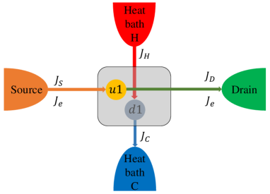
Figure 1: Schematic of four-terminal QDs thermoelectric system. Beside the source and the drain, there are two other electrodes, $H$ and $C$. Only the heat currents flowing out/into these electrodes are considered, since their electrochemical potentials are set to the equilibrium value. In experiments, these two electrodes (termed as “heat baths”) and the QD $d1$ are fabricated in a lower layer. In the upper layer, there are the source, the drain, and the QD $u1$. The lower and upper layers are separated by an insulating layer (depicted as the gray shadow). Electrons in the two QDs interact with each other via Coulomb (repulsive) interaction.

Beside the source and the drain, there are other two electrodes (electronic reservoirs). In our set-up, their electrochemical potentials are set to the equilibrium value so that they serve as “heat baths”, i.e., charge motions between them do not produce or consume any electrical energy. We thus consider only the heat current flowing out of the $H$ reservoir, $J_{H}$, and the heat current flowing into the $C$ reservoir, $J_{C}$ (we suppose $T_{H}>T_{C}$, where $T_{H}$ and $T_{C}$ are the temperature of the heat bath $H$ and $C$, respectively.). In contrast, the source and the drain can have potentials differing from the equilibrium value, leading to charge motion under (self-consistent) electrical fields. We hence consider both the charge current between the source and the drain, $J_{e}$, and the heat current flowing out of (into) the source (drain) terminal, $J_{S}$ ($J_{D}$).

Although there are four heat currents, energy conservation impose the following restriction,

$$J_{S}+\frac{\mu_{S}}{e}J_{e}+J_{H}=J_{C}+J_{D}+\frac{\mu_{D}}{e}J_{e},$$ (2)

where $\mu_{S}$ and $\mu_{D}$ are the electrochemical potentials of the source and the drain, respectively. It is useful to consider the following combinations

$$J_{in}=J_{H}-J_{C},\quad J_{q}=\frac{1}{2}(J_{H}+J_{C}).$$ (3)

Here $J_{in}$ can be understood as the total heat injected into the QDs system from the two heat baths $H$ and $C$. $J_{q}$ is regarded as the heat flow (exchange) between the reservoirs $H$ and $C$. We shall choose the independent heat currents as three of the four heat currents, e.g., $J_{S}$, $J_{in}$ and $J_{q}$. The affinities corresponding to the three heat currents and the electrical current can be found by analyzing the total entropy production Jiang (2014a); Jiang et al. (2015b),

$$\partial_{t}S_{\rm tot}=\sum_{i}J_{i}A_{i},$$ (4a)

$$A_{e}=\frac{\mu_{S}-\mu_{D}}{eT_{D}},\quad A_{S}\equiv\frac{1}{T_{D}}-\frac{1}{T_{S}},$$ (4b)

$$A_{in}\equiv\frac{1}{T_{D}}-\frac{1}{2T_{H}}-\frac{1}{2T_{C}},\quad A_{q}\equiv\frac{1}{T_{C}}-\frac{1}{T_{H}}.$$ (4c)

To demonstrate the underlying physics, in the following we shall consider the simple situation where there is only a single energy level that allows tunneling between each electrode to the connected QD.

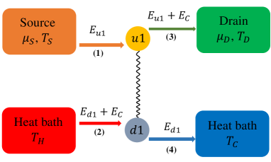
Figure 2: Illustration of correlated electron transport through the QDs $u1$ and $d1$. An electron tunnels between the source and the QD $u1$ only at energy $E_{u1}$ (i.e., when there is no electron in the QD $d1$). The electron tunnels between the drain and the QD $u1$ can only take place at energy $E_{u1}+E_{C}$ (i.e., with an electron in the QD $d1$). For the QD $d1$, electron tunnels between the heat bath $H$ and the QD only at energy $E_{d1}+E_{C}$ (i.e., when there is an electron in the QD $u1$). The electron tunnels between the QD $d1$ and the heat bath $C$ only at energy $E_{d1}$. The interaction between electron, depicted as the wavy lines, is the crucial element for the correlated inelastic transport through the QDs $u1$ and $d1$. For the electron motion indicated by the arrows, an energy $E_{C}$ is pumped into the source and drain subsystem from the $H$ and $C$ subsystem.

We now present the microscopic theory for thermoelectric transport in the QDs system. Explicitly we shall construct the expressions for the electrical and heat currents as functions of the electrochemical potentials, $\mu_{S}$ and $\mu_{D}$, as well as the temperatures, $T_{S}$, $T_{D}$, $T_{H}$ and $T_{C}$. As shown in Fig. 2, we consider particular configurations where QDs $u1$ and $d1$ are capacitively coupled, whereas there is no other coupling between QD $u1$ and other QDs. We also assume that the intradot Coulomb repulsion is so strong that double occupancy is forbidden. In such configurations, the energy for electron in the QDs are given by

$$E_{u1,n_{d1}}=E_{u1}+n_{d1}E_{C},$$ (5a)

$$E_{d1,n_{u1}}=E_{d1}+n_{u1}E_{C},$$ (5b)

$$\quad n_{u1},n_{d1}=0,1.$$ (5c)

Here $E_{u1}$ and $E_{d1}$ are the electron energies for QDs $u1$ and $d1$ if there is no interaction between QDs. $n_{u1}$ and $n_{d1}$ denote the number of electrons in the $u1$ and $d1$ QDs, respectively.

We now study the steady-state transport through $u1$ and $d1$ using the master equation method as in Ref. Sánchez and Büttiker (2011). There are four quantum states for electrons in the two QDs $u1$ and $d1$, respectively, characterized by the quantum numbers $n_{u1}$ and $n_{d1}$, and denoted as $|n_{u1},n_{d1}\rangle$. The electron density matrix of the QDs system at the steady-state is characterized by the four-component vector $\rho=(\rho_{0,0},\rho_{1,0},\rho_{0,1},\rho_{1,1})^{T}$. The steady-state transport currents are determined by the steady-state density matrix $\rho$, which is obtained by solving the master equation for steady-state, $\partial_{t}\rho=\hat{L}_{(1)}\rho=0$. Here

$$\hat{L}_{(1)}=\left(\begin{array}[]{cccc}-k_{u1,0}^{+}-k_{d1,0}^{+}&k_{u1,0}^{-}&k_{d1,0}^{-}&0\\ k_{u1,0}^{+}&-k_{u1,0}^{-}-k_{d1,1}^{+}&0&k_{d1,1}^{-}\\ k_{d1,0}^{+}&0&-k_{d1,0}^{-}-k_{u1,1}^{+}&k_{u1,1}^{-}\\ 0&k_{d1,1}^{+}&k_{u1,1}^{+}&-k_{d1,1}^{-}-k_{u1,1}^{-}\\ \end{array}\right)$$ (6)

The transition rates are

$$k_{u1,n_{d1}}^{\pm}\equiv k_{S,u1,n_{d1}}^{\pm}+k_{D,u1,n_{d1}}^{\pm},$$ (7a)

$$k_{d1,n_{u1}}^{\pm}\equiv k_{H,d1,n_{u1}}^{\pm}+k_{C,d1,n_{u1}}^{\pm},$$ (7b)

where the superscript $+$ ($-$) representing the rates for the processes with electron entering into (leaving) the QD. For the “$k$” in the right hand sides of the equations, the first two subscripts denote the reservoir and the QD as the starting or end point of the tunneling, while the third subscript denotes the number of electrons in the capacitively coupled QD (e.g., for tunneling into the QD $u1$, the capacitively coupled QD is $d1$). And

$$k_{i,u1,n_{d1}}^{+}\equiv\Gamma_{i,u1,n_{d1}}f\left(\frac{E_{u1,n_{d1}}-\mu_{i}}{k_{B}T_{i}}\right),\ \ i=S,D,$$ (8a)

$$k_{i,d1,n_{u1}}^{+}\equiv\Gamma_{i,d1,n_{u1}}f\left(\frac{E_{d1,n_{u1}}}{k_{B}T_{i}}\right),\ \ i=H,C,$$ (8b)

$$k_{i,u1,n_{d1}}^{-}\equiv\Gamma_{i,u1,n_{d1}}-k_{i,u1,n_{d1}}^{+},\ \ i=S,D,$$ (8c)

$$k_{i,d1,n_{u1}}^{-}\equiv\Gamma_{i,d1,n_{u1}}-k_{i,d1,n_{u1}}^{+},\ \ i=H,C,$$ (8d)

where $\Gamma_{i,u1,n_{d1}}$ is the tunneling rate between the reservoir $i$ and the QD $u1$ at energy $E_{u1,n_{d1}}$ (the other tunneling rates are defined similarly), and $f(x)=1/(e^{x}+1)$ is the Fermi-Dirac distribution function.

In the above equations, we have set

$$\mu_{H}=\mu_{C}\equiv 0$$ (9)

as both the equilibrium electrochemical potential and the energy zero for electrons. The tunneling rates can, in principle, be calculated via the Fermi golden rule Jiang et al. (2012, 2015a). In this work, however, we assume that they can be tuned at will in experiments (e.g., by changing the channel width of the leads, or attaching QDs that are strongly coupled with the leads; in the former we change the step-function like tunneling rates, while in the latter Lorentzian shape tunneling rates can be formed) Prete et al. (2019); Jaliel et al. (2019). It has been found that asymmetry in the tunneling rates $\Gamma_{i}$ (as functions of energy) is crucial to induce inelastic thermoelectric transport in the QDs system Sánchez and Büttiker (2011); Sothmann et al. (2012).

II.2 Four quantum-dots thermoelectric system

In order to realize the cooling by heat current effect through the Coulomb interaction, we consider the four-terminal four QDs thermoelectric system, as shown in Fig. 3(a). In this particular configurations, QDs $u2$ and $d2$ are capacitively coupled, whereas there is no other coupling between QD $u2$ and other QDs [see Fig. 3(b)].

Similarly, the expressions hold for QDs $u2$ and $d2$ are

$$E_{u2,n_{d2}}=E_{u2}+n_{d2}E_{C},$$ (10)

$$E_{d2,n_{u2}}=E_{d2}+n_{u2}E_{C},$$ (11)

$$\quad n_{u2},n_{d2}=0,1.$$ (12)

For simplicity, we have assumed that the charge interaction strength between the QDs $u2$ and $d2$ are the same as that for the QDs $u1$ and $d1$. Transport through QDs system can actually be divided into two parts: the four-terminal transport through the pair of QDs $u1$ and $d1$ and that through the pair of QDs $u2$ and $d2$. These two channels are independent of each other.

Transport equations through the other pair of QDs, $u2$ and $d2$, can be solved similarly. In fact, the matrix $\hat{L}_{(2)}$ is the same as $\hat{L}_{(1)}$ with only $u1$ replaced by $u2$ and $d1$ replaced by $d2$. We shall use the vector $\rho^{\prime}=(\rho^{\prime}_{0,0},\rho^{\prime}_{1,0},\rho^{\prime}_{0,1},\rho^{\prime}_{1,1})^{T}$ to represent the density matrix of electrons in the QDs $u2$ and $d2$ at the transport steady-state. Here each element of the density matrix $\rho^{\prime}_{n_{u2}n_{d2}}$ carries the index characterizing the quantum states of electrons in the QDs $u2$ and $d2$, $|n_{u2},n_{d2}\rangle$.

After numerically solving the master equations at the steady-state transport Sánchez and Büttiker (2011)

$$\hat{L}_{(1)}\rho=0,\quad\hat{L}_{(2)}\rho^{\prime}=0,$$ (13)

one can determine the steady-state transport currents from $\rho$ and $\rho^{\prime}$ as,

$$J_{e}=\sum_{n_{d1}}e(k_{S,u1,n_{d1}}^{+}\rho_{0,n_{d1}}-k_{S,u1,n_{d1}}^{-}\rho_{1,n_{d1}})+\sum_{n_{d2}}e(k_{S,u2,n_{d2}}^{+}\rho^{\prime}_{0,n_{d2}}-k_{S,u2,n_{d2}}^{-}\rho^{\prime}_{1,n_{d2}}),$$ (14a)

$$J_{S}=\sum_{n_{d1}}(E_{u1,n_{d1}}-\mu_{S})(k_{S,u1,n_{d1}}^{+}\rho_{0,n_{d1}}-k_{S,u1,n_{d1}}^{-}\rho_{1,n_{d1}})+\sum_{n_{d2}}(E_{u2,n_{d2}}-\mu_{S})(k_{S,u2,n_{d2}}^{+}\rho^{\prime}_{0,n_{d2}}-k_{S,u2,n_{d2}}^{-}\rho^{\prime}_{1,n_{d2}}),$$ (14b)

$$J_{H}=\sum_{n_{u1}}E_{d1,n_{u1}}(k_{H,d1,n_{u1}}^{+}\rho_{n_{u1},0}-k_{H,d1,n_{u1}}^{-}\rho_{n_{u1},1})+\sum_{n_{u2}}E_{d2,n_{u2}}(k_{H,d2,n_{u2}}^{+}\rho^{\prime}_{n_{u2},0}-k_{H,d2,n_{u2}}^{-}\rho^{\prime}_{n_{u2},1}),$$ (14c)

$$J_{C}=\sum_{n_{u1}}E_{d1,n_{u1}}(k_{C,d1,n_{u1}}^{-}\rho_{n_{u1},1}-k_{C,d1,n_{u1}}^{+}\rho_{n_{u1},0})+\sum_{n_{u2}}E_{d2,n_{u2}}(k_{C,d2,n_{u2}}^{-}\rho^{\prime}_{n_{u2},1}-k_{C,d2,n_{u2}}^{+}\rho^{\prime}_{n_{u2},0}).$$ (14d)

We can obtain $J_{in}$ and $J_{q}$ from the two currents, $J_{H}$ and $J_{C}$.

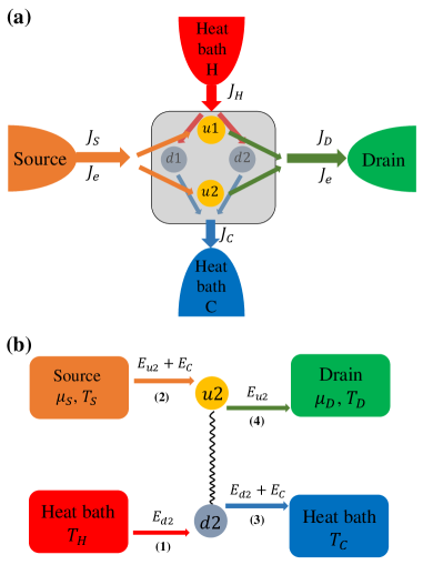
Figure 3: (a) Schematic of four-terminal QDs thermoelectric system. Beside the source and the drain, there are two other electrodes. Only the heat currents flowing out/in these electrodes are considered, since their electrochemical potentials are set to the equilibrium value. In experiments, these two electrodes (termed as “heat baths”) and the two QDs $d1$ and $d2$ can be fabricated in a lower layer. The source and drain electrodes together with the QDs $u1$ and $u2$ can be fabricated in the upper layer. The lower layer and the upper layer are separated by an insulating layer (depicted as the gray shadow). But electrons in the QDs can interact with each other via the long range Coulomb interaction. (b) Correlated electron tunneling through the QDs $u2$ and $d2$. Similar to electron tunneling through the $u1$ and $d1$ QDs, but with different energy configuration for electron tunneling. For electron motion indicated by the arrows in the figure, an energy $E_{C}$ is provided by the source and drain subsystem to the $H$ and $C$ subsystem. The arrows indicate one possible direction of electron motion, which can be reversed, depending on the voltage and temperature biases. The numbers in the brackets indicate the sequences of the correlated tunneling processes.

II.3 Inelastic thermoelectric transport through correlated tunneling

We now study a special configuration that allows unconventional thermoelectric transport through drag effects. In this configuration, we choose the following tunneling rates,

$$\Gamma_{S,u1,n_{d1}=0}=\Gamma_{0},\quad\Gamma_{S,u1,n_{d1}=1}=0,$$ (15)

$$\Gamma_{D,u1,n_{d1}=0}=0,\quad\Gamma_{D,u1,n_{d1}=1}=\Gamma_{0},$$

$$\Gamma_{H,d1,n_{u1}=0}=0,\quad\Gamma_{H,d1,n_{u1}=1}=\Gamma_{0},$$

$$\Gamma_{C,d1,n_{u1}=0}=\Gamma_{0},\quad\Gamma_{C,d1,n_{u1}=1}=0;$$

$$\Gamma_{S,u2,n_{d2}=0}=0,\quad\Gamma_{S,u2,n_{d2}=1}=\Gamma_{0},$$

$$\Gamma_{D,u2,n_{d2}=0}=\Gamma_{0},\quad\Gamma_{D,u2,n_{d2}=1}=0,$$

$$\Gamma_{H,d2,n_{u2}=0}=\Gamma_{0},\quad\Gamma_{H,d2,n_{u2}=1}=0,$$

$$\Gamma_{C,d2,n_{u2}=0}=0,\quad\Gamma_{C,d2,n_{u2}=1}=\Gamma_{0},$$

where $\Gamma_{0}$ is a constant for the tunneling rates. The above configuration is schematically illustrated in Fig. 2 and Fig. 3(b). For such a configuration, in the QDs $u1$ and $d1$ only the following process of electron motion (and its time-reversal) is possible,

$$|0,0\rangle\xrightarrow[QD\ u1:\ E_{u1}]{\Gamma_{S,u1,0}}|1,0\rangle\xrightarrow[QD\ d1:\ E_{d1}+E_{C}]{\Gamma_{H,d1,1}}|1,1\rangle$$ (16)

$$\xrightarrow[QD\ u1:\ E_{u1}+E_{C}]{\Gamma_{D,u1,1}}|0,1\rangle\xrightarrow[QD\ d1:\ E_{d1}]{\Gamma_{C,d1,0}}|0,0\rangle.$$

The above expression represents the correlated electron tunneling through the QDs $u1$ and $d1$. The quantum states are labeled by the two integers $n_{u1},n_{d1}$. In the above expression, below each arrow is the QD of which electron is tunneling into or outside and the energy of the electron that tunnels, while above each arrow is the tunneling rate. The consequence of the above correlated tunneling processes is an electron traverses from the $H$ reservoir to the $C$ reservoir via the QD $d1$, in the meanwhile an electron traverses from the source to the drain via the QD $u1$. The interaction between the electrons in the two QDs provides the mechanism for passing energy between the two channels. The electron traverse from $H$ to $C$ loses energy $E_{C}$, while the electron traverses from the source to the drain and gains energy $E_{C}$. The above correlated tunneling processes, as the only passage for electron transport through the QDs $u1$ and $d1$, also dictates the direction correlation between the electron flowing in the two channels: when an electron goes from $H$ to $C$, there has to be an electron moving from the source to the drain, otherwise the energy is not conserved! Such locking between electron motions in the two channels is the key for the unconventional thermoelectric transport in our system.

Similarly, for transport through the QDs $u2$ and $d2$, only the following process and its time-reversal is allowed,

$$|0,0\rangle\xrightarrow[QD\ d2:\ E_{d2}]{\Gamma_{H,d2,0}}|0,1\rangle\xrightarrow[QD\ u2:\ E_{u2}+E_{C}]{\Gamma_{S,u2,1}}|1,1\rangle$$ (17)

$$\xrightarrow[QD\ d2:\ E_{d2}+E_{C}]{\Gamma_{C,d2,1}}|1,0\rangle\xrightarrow[QD\ u2:\ E_{u2}]{\Gamma_{D,u2,0}}|0,0\rangle.$$

Each time the above process (the reversed process) takes place, an electron traverse from $H$ to $C$, and another electron traverse from the source to the drain. There are always an equal number of electrons traveling from $H$ to $C$ as the number of electrons traveling from the source to the drain.

According to the above picture, the electrical and heat currents can be expressed as

$$J_{e}=e\sum I_{i},$$ (18a)

$$J_{S}=E_{u1}I_{1}+(E_{u2}+E_{C})I_{2},$$ (18b)

$$J_{H}=(E_{d1}+E_{C})I_{1}+E_{d2}I_{2},$$ (18c)

$$J_{C}=E_{d1}I_{1}+(E_{d2}+E_{C})I_{2},$$ (18d)

$$J_{in}=E_{C}(I_{1}-I_{2}),$$ (18e)

$$J_{q}=(E_{d1}+\frac{1}{2}E_{C})I_{1}+(E_{d2}+\frac{1}{2}E_{C})I_{2},$$ (18f)

where

$$I_{1}=\gamma_{1}^{-1}(k^{+}_{u1,0}k^{+}_{d1,1}k^{-}_{u1,1}k^{-}_{d1,0}-k^{+}_{d1,0}k^{+}_{u1,1}k^{-}_{d1,1}k^{-}_{u1,0}),$$ (19a)

$$I_{2}=\gamma_{2}^{-1}(k^{+}_{d2,0}k^{+}_{u2,1}k^{-}_{d2,1}k^{-}_{u2,0}-k^{+}_{u2,0}k^{+}_{d2,1}k^{-}_{u2,1}k^{-}_{d2,0}),$$ (19b)

are the electron number current through the QD $u1$ (or $d1$), and the electron number current through the QD $u2$ (or $d2$), respectively. According to Ref. Sánchez and Büttiker (2011),

$$\gamma_{1}= \sum_{\alpha=u1,d1}\sum_{i=\pm}\sum_{n=0,1}k^{-i}_{\alpha,n}(k^{i}_{\alpha,1-n}k^{i}_{-\alpha,n}$$ (20)

$$+k^{-i}_{-\alpha,n}\sum_{j}k^{j}_{-\alpha,n}\delta_{|1+i|,2n}),$$

$$\gamma_{1}= \sum_{\alpha=u2,d2}\sum_{i=\pm}\sum_{n=0,1}k^{-i}_{\alpha,n}(k^{i}_{\alpha,1-n}k^{i}_{-\alpha,n}$$

$$+k^{-i}_{-\alpha,n}\sum_{j}k^{j}_{-\alpha,n}\delta_{|1+i|,2n}),$$

where $-u1=d1$ and $-u2=d2$. From the relations between currents we can also obtain the relations between the linear-response transport coefficients. If $I_{i}=\sum_{j}M_{ij}A_{j}$ ($i,j=e,S,in,q$) where $M_{ij}$ are the linear-response transport coefficients, then

$$M_{e,e}=TG,\quad M_{e,S}=e^{-1}TG\left[p_{1}E_{u1}+p_{2}(E_{u2}+E_{C})\right],\quad M_{e,in}=e^{-1}TGE_{C}(p_{1}-p_{2}),$$ (21a)

$$M_{e,q}=e^{-1}TG\left[p_{1}E_{d1}+p_{2}E_{d2}+\frac{1}{2}E_{C}\right],\quad M_{S,S}=e^{-2}TG\left[p_{1}E_{u1}^{2}+p_{2}(E_{u2}+E_{C})^{2}\right],$$ (21b)

$$M_{S,in}=e^{-2}TG\left[p_{1}E_{u1}E_{C}-p_{2}(E_{u2}+E_{C})E_{C}\right],$$ (21c)

$$M_{S,q}=e^{-2}TG\left[p_{1}E_{u1}(E_{d1}+\frac{1}{2}E_{C})+p_{2}(E_{u2}+E_{C})(E_{d2}+\frac{1}{2}E_{C})\right],$$ (21d)

$$M_{in,in}=e^{-2}TGE_{C}^{2},\quad M_{in,q}=e^{-2}TG\left[p_{1}E_{C}(E_{d1}+\frac{1}{2}E_{C})-p_{2}E_{C}(E_{d2}+\frac{1}{2}E_{C})\right],$$ (21e)

$$M_{q,q}=e^{-2}TG\left[p_{1}(E_{d1}+\frac{1}{2}E_{C})^{2}+p_{2}(E_{d2}+\frac{1}{2}E_{C})^{2}\right]$$ (21f)

where $G$ is the total conductance, and $p_{i}=G_{i}/G$ ($i=1,2$) with $G_{i}$ being the conductance for the transport through the QDs pair $u1$ and $d1$ (if $i=1$) or that for the transport through the QDs pair $u2$ and $d2$ (if $i=2$).

II.4 Unconventional Thermoelectric energy conversion

There are three different types of thermoelectric effects, associated with the following Seebeck coefficients Jiang (2014b); Lu et al. (2017),

$$S_{S}=\frac{M_{e,S}}{T^{2}G}=\frac{k_{B}}{e}\frac{\langle a_{S}\rangle}{k_{B}T},$$ (22a)

$$S_{in}=\frac{M_{e,in}}{T^{2}G}=\frac{k_{B}}{e}\frac{\langle a_{in}\rangle}{k_{B}T},$$ (22b)

$$S_{q}=\frac{M_{e,q}}{T^{2}G}=\frac{k_{B}}{e}\frac{\langle a_{q}\rangle}{k_{B}T},$$ (22c)

where

$$\langle{\cal O}\rangle=\sum_{i=1,2}p_{i}{\cal O}_{i}$$ (23a)

$$a_{S,1}=E_{u1},\quad a_{S,2}=E_{u2}+E_{C},$$ (23b)

$$a_{in,1}=E_{C},\quad a_{in,2}=-E_{C},$$ (23c)

$$a_{q,1}=E_{d1}+\frac{1}{2}E_{C},\quad a_{q,2}=E_{d2}+\frac{1}{2}E_{C}.$$ (23d)

In our system which breaks the left-right inversion symmetry and up-down inversion symmetry [see Eq. (15)], if $p_{1}=p_{2}$, the Seebeck coefficient $S_{in}$ vanishes. The other two Seebeck coefficients are nonzero even at the particle-hole symmetric limit with $E_{u1}=E_{d1}=E_{u2}=E_{d2}=0$. The figures of merit for these three thermoelectric effects can be expressed as

$$Z_{S}T=\frac{\langle a_{S}\rangle^{2}}{\langle a_{S}^{2}\rangle-\langle a_{S}\rangle^{2}},$$ (24a)

$$Z_{in}T=\frac{\langle a_{in}\rangle^{2}}{\langle a_{in}^{2}\rangle-\langle a_{in}\rangle^{2}},$$ (24b)

$$Z_{q}T=\frac{\langle a_{q}\rangle^{2}}{\langle a_{q}^{2}\rangle-\langle a_{q}\rangle^{2}}.$$ (24c)

These figures of merit can be rather high when the variances of $a_{S}$, $a_{in}$, and $a_{q}$ are small.

III Cooling by thermal current

We now study the cooling by thermal current effect, i.e., cooling the source (i.e., $J_{S}>0$ even though $T_{S}<T_{D}$ and $A_{S}<0$) as driven by the thermal current $J_{q}$ when

$$\mu_{S}=\mu_{D}=0,\quad{\rm i.e.},\quad A_{e}=0,$$ (25a)

$$T_{C}=\frac{1}{\frac{2}{T_{D}}-\frac{1}{T_{H}}},\quad{\rm i.e.},\quad A_{in}=0.$$ (25b)

We consider the situations with $T_{H}>T_{D}>T_{C}$. $T_{D}$ is the reference temperature that may be set by the substrate. This effect can take place only when $J_{q}A_{q}>0$, i.e., the negative entropy production (i.e., positive free energy production) during the cooling of the source is compensated by the positive entropy production during the thermal conduction $J_{q}$ (i.e., free energy consumption, $J_{q}A_{q}>0$), so that the total entropy production is non-negative, Kedem and Caplan (1965); Jiang (2014a)

$$\partial_{t}S_{\rm tot}=J_{q}A_{q}+J_{S}A_{S}\geq 0.$$ (26)

In the linear-response regime, to have $J_{S}>0$ while $A_{S}<0$, one needs a positive and large enough $M_{S,q}$.

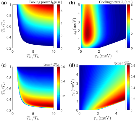
Figure 4: (a) Cooling power $J_{S}$ as functions of temperature ratios $T_{S}/T_{D}$ and $T_{H}/T_{D}$ for $E_{u1}=E_{u2}=E_{d1}=E_{d2}=1$ meV. (b) Cooling power $J_{S}$ as functions of QDs energies $E_{u1}=E_{u2}=\varepsilon_{u}$ and $E_{d1}=E_{d2}=\varepsilon_{d}$ for $k_{B}T_{H}=6$ meV and $k_{B}T_{S}=0.6$ meV. (c) The COP ratio $\eta_{\rm COP}/\eta_{\rm COP}^{\rm rev}$ for the cooling by thermal current effect as functions of the temperature ratios $T_{S}/T_{D}$ and $T_{H}/T_{D}$ when QDs energy is the same as in (a). (d) $\eta_{\rm COP}/\eta_{\rm COP}^{\rm rev}$ as functions of QDs energies $\varepsilon_{u}$ and $\varepsilon_{d}$ for the same parameters as in (b). Common parameters: $\mu_{S}=\mu_{D}=0$, $k_{B}T_{D}=1$ meV, $T_{C}=1/(2/T_{D}-1/T_{H})$, $\Gamma_{0}=0.1$ meV, and $E_{C}=2$ meV.

The coefficient of performance (COP) for the cooling by thermal current effect is given by the ratio of the two heat currents

$$\eta_{\rm COP}=\frac{J_{S}}{J_{q}}=\frac{E_{u1}I_{1}+(E_{u2}+E_{C})I_{2}}{(E_{d1}+\frac{1}{2}E_{C})I_{1}+(E_{d2}+\frac{1}{2}E_{C})I_{2}}.$$ (27)

From Eq. (26) and the definition of the COP we find that

$$\eta_{\rm COP}=\left(T_{S}A_{q}-\frac{T_{S}{\partial_{t}}S_{\rm tot}}{J_{q}}\right)\frac{T_{D}}{T_{D}-T_{S}}.$$ (28)

The reversible COP is

$$\eta^{\rm rev}_{\rm COP}=\left(\frac{T_{S}}{T_{C}}-\frac{T_{S}}{T_{H}}\right)\frac{T_{D}}{T_{D}-T_{S}}=-\frac{A_{q}}{A_{S}}.$$ (29)

We regard $T_{D}$ as the reference temperature fixed by the substrate and $T_{C}$ as determined by Eq. (25b), so that only the temperatures $T_{S}$ and $T_{H}$ are independent variables. The working condition for the cooling driven by the thermal current $J_{q}$ is restricted by

$$0\leq\eta_{\rm COP}\leq-\frac{A_{q}}{A_{S}}.$$ (30)

At reversible COP $\eta^{\rm rev}_{\rm COP}=-\frac{A_{q}}{A_{S}}$ the cooling power vanishes, since the entropy production and the currents vanish Kedem and Caplan (1965); Entin-Wohlman et al. (2014); Jiang (2014a).

In Fig. 4(a) the cooling power of our nonelectric refrigerator is large when the temperature of the source $T_{S}$ is close to the temperature of drain $T_{D}$ and when the temperature of the heat bath $T_{H}$ is much higher than the temperature of the drain, $T_{H}\gg T_{D}$. From Fig. 4(a) the lowest temperature of the source $T_{S}$ that can be cooled down is about $0.25T_{D}$. In the white region the device cannot function as a refrigerator. As shown in Fig. 3(b), for a given temperature of $T_{H}=6T_{D}$ and $T_{S}=0.6T_{D}$, the cooling power is large for $E_{u1}=E_{u2}=\varepsilon_{u}$ around $k_{B}T_{D}$ ($k_{B}T_{D}=1$ meV throughout this paper), particularly when $\varepsilon_{d}\gtrsim\varepsilon_{u}$. In Fig. 4(c) the ratio of the COP over the reversible COP $\eta_{\rm COP}/\eta_{\rm COP}^{\rm rev}$ is high when the temperature of the source $T_{S}$ is low. This is the regime where the cooling power is rather low. Similarly, as shown in Fig. 4(d), the COP ratio $\eta_{\rm COP}/\eta_{\rm COP}^{\rm rev}$ is high when $\varepsilon_{d}$ is small, where the cooling power is very low. The COP can be quite a considerable fraction of the reversible COP, indicating the coupling is strong and the dissipation is low for such optimized efficiency conditions Entin-Wohlman et al. (2014). This phenomenon that the efficiency is optimized when the output power is low (for small dissipations), known as the efficiency-power trade-off, is consistent with the existing literature Entin-Wohlman et al. (2014); Jiang (2014a); Lu et al. (2019b).

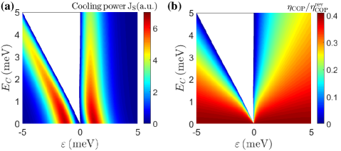
Figure 5: (a) Cooling power $J_{S}$ and (b) COP ratio $\eta_{\rm COP}/\eta_{\rm COP}^{\rm rev}$ as functions of the QDs energies $E_{u1}=E_{u2}=E_{d1}=E_{d2}=\varepsilon$ and $E_{C}$. Other parameters: $\mu_{S}=\mu_{D}=0$, $k_{B}T_{D}=1$ meV, $k_{B}T_{H}=6$ meV, $k_{B}T_{S}=0.6$ meV, $T_{C}=1/(2/T_{D}-1/T_{H})$, and $\Gamma_{0}=0.1$ meV.

We now study more on the QDs energy dependence of the cooling power $J_{S}$ and the COP ratio $\eta_{\rm COP}/\eta_{\rm COP}^{\rm rev}$ for several different configurations. We first consider the case with $E_{u1}=E_{u2}=E_{d1}=E_{d2}=\varepsilon$ and study how the energy $\varepsilon$ and the charge interaction energy $E_{C}$ affect the power and the COP. First the cooling by thermal current effect holds for all $E_{C}>0$ when $\varepsilon>0$. However, as shown in Fig. 5(a), for $\varepsilon<0$, the cooling by thermal current effect holds only when $E_{C}<-\varepsilon$. This is because in this regime, $M_{S,q}=e^{-2}TG[p_{1}\varepsilon(\varepsilon+\frac{1}{2}E_{C})+p_{2}(\varepsilon+E_{C})(\varepsilon+\frac{1}{2}E_{C})]$. The condition for positive $M_{S,q}$ holds when $E_{C}<-\varepsilon$. From Figs. 5(a) and 5(b), we note that the optimal parameters for both COP and cooling power can be $\varepsilon\sim k_{B}T_{D}$ and $E_{C}\sim k_{B}T_{D}$, or $\varepsilon\sim-2k_{B}T_{D}$ and $E_{C}\sim k_{B}T_{D}$ ($k_{B}T_{D}=1$ meV). Although the COP ratio increases with decreasing $E_{C}$ for any given $\varepsilon$, the limit with $E_{C}\to 0$ does not validate our theory.

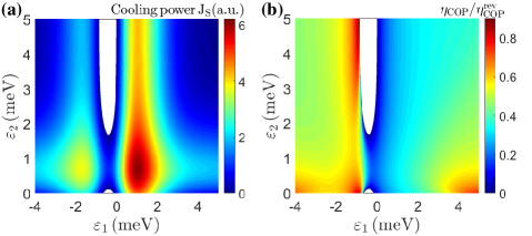
Figure 6: (a) Cooling power $J_{S}$ and (b) COP ratio $\eta_{\rm COP}/\eta_{\rm COP}^{\rm rev}$ as functions of the QDs energies $E_{u1}=E_{d1}=\varepsilon_{1}$ and $E_{u2}=E_{d2}=\varepsilon_{2}$. Other parameters: $\mu_{S}=\mu_{D}=0$, $k_{B}T_{D}=1$ meV, $k_{B}T_{H}=6$ meV, $k_{B}T_{S}=0.6$ meV, $T_{C}=1/(2/T_{D}-1/T_{H})$, $E_{C}=1$ meV, and $\Gamma_{0}=0.1$ meV.

If we allow the energy configuration to be different between the pair of QDs $u1$ and $d1$ and the other pair of QDs $u2$ and $d2$ in a way that $E_{u1}=E_{d1}=\varepsilon_{1}$ and $E_{u2}=E_{d2}=\varepsilon_{2}$ with $E_{C}=1$ meV, we can study how the cooling performance varies with the energies in the two channels, $\varepsilon_{1}$ and $\varepsilon_{2}$. From the Fig. 6(a), we find that the cooling power is maximized at $\varepsilon_{1}\sim\varepsilon_{2}\sim 1$ meV. As shown in Fig. 6(b), the COP ratio is rather optimized when $\varepsilon_{1}\sim-1$ meV for large $\varepsilon_{2}$. This observation again demonstrates the efficiency-power trade off Entin-Wohlman et al. (2014); Jiang (2014a); Lu et al. (2019b).

IV Four-terminal thermoelectric system as a Maxwell’s demon

Maxwell’s demon is a hypothetical demon, which can detect and control the motion of a single molecule. It was conceived by James Clerk Maxwell in 1871 to explain the possibility of violating the second law of thermodynamics. The demon is assumed to control a door, which separates two boxes to realize the non-equilibrium gas distribution Maxwell (1871). This operation that appeared to be in violation of the second law of thermodynamics, decreasing the entropy of the gas without any work input. Despite the complexity, such Maxwell’s demon has been realized in various systems in different forms Koski et al. (2014a, 2015, b); Chida et al. (2017). For example, the QD multi-terminal systems can be possibly realized as a Maxwell’s demon by using the inelastic transport without any measurement of individual particles or any feedback involved Sánchez et al. (2019a, b); Annby-Andersson et al. (2020); Lu et al. (2021).

As shown in Fig. 7, here we introduce a Maxwell’s demon based on two electronic thermal baths (the hot bath $H$ and cold bath $C$) which can reduce the entropy of the working substance (the source and the drain), without changing the energies and particles of the working substance. The nonequilibrium Maxwell’s demon is used to reverse the natural direction of the source and drain where the drain has a higher temperature. As we introduced in the previous section, when we realize the cooling by thermal current effect, the entropy of the source and drain is reduced, while the entropy of the whole thermoelectric system is increased. This operation seemingly break the the second law of thermodynamics, the entropy production of the two heat baths $H$ and $C$ compensates for that of the source and drain.

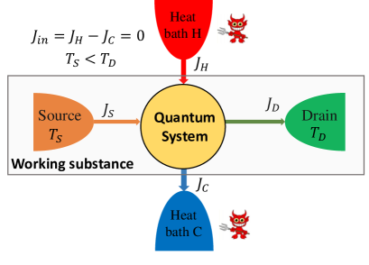
Figure 7: Illustration of a four-terminal mesoscopic thermoelectric device as a Maxwell demon. The Maxwell’s demon does not supply any energy to the working substance, i.e., the total heat current injected into the central quantum system from the two thermal baths is zero, $J_{in}=J_{H}-J_{C}=0$.

The condition at which the Maxwell’s demon neither injects nor extracts heat or energy into the working substance is Lu et al. (2021)

$$J_{in}\,=\,0.$$ (31)

The power of the Maxwell demon vanishes when the temperature gradient between the two heat baths $H$ and $C$ is vanishing.

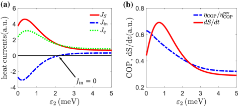
Figure 8: (a) Cooling power $J_{S}$, the total injected heat $J_{in}$, and the thermal current $J_{q}$ as a function of the QD energy $E_{u2}=E_{d2}=\varepsilon_{2}$. (b) COP ratio $\eta_{\rm COP}/\eta_{\rm COP}^{\rm rev}$, entropy production rate $\partial_{t}S_{\rm tot}$ as a function of the QDs energy $E_{u2}=E_{d2}=\varepsilon_{2}$. Other parameters: $\mu_{S}=\mu_{D}=0$, $k_{B}T_{D}=1$ meV, $k_{B}T_{H}=6$ meV, $k_{B}T_{S}=0.6$ meV, $T_{C}=1/(2/T_{D}-1/T_{H})$, $E_{u1}=E_{d1}=\varepsilon_{1}=4$ meV, $E_{C}=2$ meV, and $\Gamma_{0}=0.1$ meV.

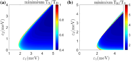
Figure 9: (a) The lowest temperature of source $T_{S}$ that can be cooled down via the cooling by transverse current effect as functions of the QDs energies $\varepsilon_{1}$ and $\varepsilon_{2}$ for $k_{B}T_{H}=6$ meV and $J_{in}=0$. (b) The lowest temperature of the hot heat bath T H that can perform the cooling by transverse current effect as functions of the QDs energies $\varepsilon_{1}$ and $\varepsilon_{2}$ for $k_{B}T_{S}=0.6$ meV and $J_{in}=0$.

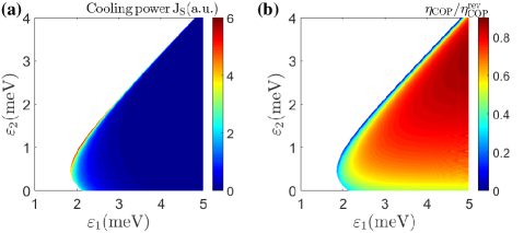
Figure 10: (a) Cooling power $J_{S}$ and (b) COP ratio $\eta_{\rm COP}/\eta_{\rm COP}^{\rm rev}$ as functions of the QDs energies $E_{u1}=E_{d1}=\varepsilon_{1}$ and $E_{u2}=E_{d2}=\varepsilon_{2}$ for $J_{in}=0$. Other parameters: $\mu_{S}=\mu_{D}=0$, $k_{B}T_{D}=1$ meV, $k_{B}T_{H}=6$ meV, $T_{C}=1/(2/T_{D}-1/T_{H})$, $E_{C}=1$ meV, and $\Gamma_{0}=0.1$ meV.

In Fig. 8, we show that in our system it is indeed possible to realize the cooling by thermal current with vanishing total injected heat, $J_{in}=0$. We find that the cooling by thermal current effect emerges in the whole region of $0\leq\varepsilon_{2}\leq 5$ meV, regardless of the sign change and the vanishing of the total heat injected into the QDs $u1$ and $d1$ from the two heat baths $H$ and $C$.

Under the condition of Maxwell’s demon, $J_{in}=0$, we then begin to study the optimal energy configuration for the QD energies, $E_{u1}=E_{d1}=\varepsilon_{1}$ and $E_{u2}=E_{d2}=\varepsilon_{2}$ to obtain the lowest temperature of the source and the heat bath $H$. From Fig. 9(a), we find that the lowest temperature $T_{S}$ when $\varepsilon_{1}>\varepsilon_{2}$ and $\varepsilon_{1}\geq 2$ meV. The white areas represent the parameter regions where the Maxwell’s demon effect cannot be achieved, i.e., $J_{S}<0$. Similarly, we also study the minimum temperature of the heat bath $H$ under the requirement of Maxwell’s demon. In Fig. 9(b) we can see that it does not require too high temperature of the heat bath $H$ in order to achieve the Maxwell’s demon effect in the region $\varepsilon_{1}>\varepsilon_{2}$. Meanwhile, we also find that the optimal parameter region for realization of Maxwell’s demon effect is that $\varepsilon_{1}>\varepsilon_{2}$ from Figs. 9(a) and 9(b).

In Fig. 10, we show the cooling power $J_{S}$ and COP for the cooling by thermal current effect $\eta_{\rm COP}$ as functions of QD energies $\varepsilon_{1}$ and $\varepsilon_{2}$ for $J_{in}=0$. In accordance with Figure 9, the maximum of the cooling efficiency can be achieved when $\varepsilon_{1}>\varepsilon_{2}$ but the value of the power is small. The results are consistent with the trade-off of power and efficiency Jiang (2014a); Proesmans et al. (2016); Lu et al. (2019b).

V conclusion and discussions

In this work, we have demonstrated a mode of the cooling by thermal current effect, the transverse thermoelectric effect and Maxwell’s demon effect, through a four-terminal four QDs thermoelectric device (the four terminals are the source, the drain and two electronic thermal baths, respectively). We have demonstrated that the Coulomb interaction between the two circuits separated by an insulating layer is the key factor and the inelastic thermoelectric transport in the two circuits leading to these two unconventional thermoelectric effects. The source can be cooled by passing a thermal current between the two electronic heat baths.

Besides, we studied the Onsager linear-response relations, the Seebeck efficient and the figure of merits of the four-terminal devices. We investigated the relationships between the power and efficiency in the linear or nonlinear response regime.

In addition, we also showed that the two thermal baths can be exploited for power generation and cooling the low-temperature heat bath (or heating the high-temperature heat bath) in a demonlike way, where the working substance does not exchange any energy or particle with the two thermal baths. Our study may be beneficial for autonomous and energy-efficient electric application on the nanoscale devices.

VI Acknowledgment

M.X. and T.Y. acknowledge support from the Science and Technological Fund of Anhui Province for Outstanding Youth (Grant No. 1508085J02), the National Natural Science Foundation of China (Grant No.61475004) and the Chinese Academy of Sciences (Grant No.XDA04030213). R.W. J.L and J.-H.J acknowledge support from the National Natural Science Foundation of China (NSFC Grant No. 11675116, No. 12074281), the Jiangsu distinguished professor funding and a Project Funded by the Priority Academic Program Development of Jiangsu Higher Education Institutions (PAPD). J.L also acknowledges support from the China Postdoctoral Science Foundation (Grant No. 2020M681376).

References

- Chen (2005) G. Chen, Nanoscale Energy Transport and Conversion (Oxford University Press, London, 2005).
- Dubi and Di Ventra (2011) Y. Dubi and M. Di Ventra, “Heat flow and thermoelectricity in atomic and molecular junctions,” Rev. Mod. Phys. 83, 131–155 (2011).
- Jiang and Imry (2016) J.-H. Jiang and Y. Imry, “Linear and nonlinear mesoscopic thermoelectric transport with coupling with heat baths,” C. R. Phys. 17, 1047 – 1059 (2016).
- Benenti et al. (2017) G. Benenti, G. Casati, K. Saito, and R. S. Whitney, “Fundamental aspects of steady-state conversion of heat to work at the nanoscale,” Phys. Rep. 694, 1 – 124 (2017).
- Sivan and Imry (1986) U. Sivan and Y. Imry, “Multichannel landauer formula for thermoelectric transport with application to thermopower near the mobility edge,” Phys. Rev. B 33, 551–558 (1986).
- Mahan and Sofo (1996) G. D. Mahan and J. O. Sofo, “The best thermoelectric,” Proc. Natl. Acad. Sci. USA 93, 7436–7439 (1996).
- (7) H. J Goldsmid, Introduction to Thermoelectricity (Springer, 2010).
- Venkatasubramanian et al. (2001) R. Venkatasubramanian, E. Silvola, T. Colpitts, and B. O’Quinn, “Thin-film thermoelectric devices with high room-temperature figures of merit,” Nature 413, 597–602 (2001).
- Giazotto et al. (2006) F. Giazotto, T. T. Heikkilä, A. Luukanen, A. M. Savin, and J. P. Pekola, “Opportunities for mesoscopics in thermometry and refrigeration: Physics and applications,” Rev. Mod. Phys. 78, 217–274 (2006).
- Jiang et al. (2006) J. H. Jiang, M. Q. Weng, and M. W. Wu, “Intense terahertz laser fields on a quantum dot with rashba spin-orbit coupling,” J. Appl. Phys. 100, 063709 (2006).
- Humphrey and Linke (2005) T. E. Humphrey and H. Linke, “Reversible thermoelectric nanomaterials,” Phys. Rev. Lett. 94, 096601 (2005).
- Zhou et al. (2011) J. Zhou, R. Yang, G. Chen, and M. S. Dresselhaus, “Optimal bandwidth for high efficiency thermoelectrics,” Phys. Rev. Lett. 107, 226601 (2011).
- Lu et al. (2017) J. Lu, R. Wang, Y. Liu, and J.-H. Jiang, “Thermoelectric cooperative effect in three-terminal elastic transport through a quantum dot,” J. Appl. Phys. 122, 044301 (2017).
- Sánchez and Serra (2011) D. Sánchez and L. Serra, “Thermoelectric transport of mesoscopic conductors coupled to voltage and thermal probes,” Phys. Rev. B 84, 201307 (2011).
- Sánchez and Büttiker (2011) R. Sánchez and M. Büttiker, “Optimal energy quanta to current conversion,” Phys. Rev. B 83, 085428 (2011).
- Sánchez and López (2013) D. Sánchez and R. López, “Scattering theory of nonlinear thermoelectric transport,” Phys. Rev. Lett. 110, 026804 (2013).
- Simine and Segal (2012) L. Simine and D. Segal, “Vibrational cooling, heating, and instability in molecular conducting junctions: full counting statistics analysis,” Phys. Chem. Chem. Phys. 14, 13820–13834 (2012).
- Jiang et al. (2012) J.-H. Jiang, O. Entin-Wohlman, and Y. Imry, “Thermoelectric three-terminal hopping transport through one-dimensional nanosystems,” Phys. Rev. B 85, 075412 (2012).
- Jordan et al. (2013) A. N. Jordan, B. Sothmann, R. Sánchez, and M. Büttiker, “Powerful and efficient energy harvester with resonant-tunneling quantum dots,” Phys. Rev. B 87, 075312 (2013).
- Sothmann et al. (2015) B. Sothmann, R. Sánchez, and A. N Jordan, “Thermoelectric energy harvesting with quantum dots,” Nanotechnology 26, 032001 (2015).
- Li and Jiang (2016) L. Li and J.-H. Jiang, “Staircase quantum dots configuration in nanowires for optimized thermoelectric power,” Sci. Rep. 6, 31974 (2016).
- Agarwalla et al. (2017) B. K. Agarwalla, J.-H. Jiang, and D. Segal, “Quantum efficiency bound for continuous heat engines coupled to noncanonical reservoirs,” Phys. Rev. B 96, 104304 (2017).
- Wang et al. (2018) R. Wang, J. Lu, C. Wang, and J.-H. Jiang, “Nonlinear effects for three-terminal heat engine and refrigerator,” Sci. Rep. 8, 2607 (2018).
- Jiang and Imry (2017) J.-H. Jiang and Y. Imry, “Enhancing thermoelectric performance using nonlinear transport effects,” Phys. Rev. Applied 7, 064001 (2017).
- Jiang and Imry (2018) J.-H. Jiang and Y. Imry, “Near-field three-terminal thermoelectric heat engine,” Phys. Rev. B 97, 125422 (2018).
- Lu et al. (2019a) J. Lu, R. Wang, J. Ren, M. Kulkarni, and J.-H. Jiang, “Quantum-dot circuit-qed thermoelectric diodes and transistors,” Phys. Rev. B 99, 035129 (2019a).
- Mari and Eisert (2012) A. Mari and J. Eisert, “Cooling by heating: Very hot thermal light can significantly cool quantum systems,” Phys. Rev. Lett. 108, 120602 (2012).
- Cleuren et al. (2012) B. Cleuren, B. Rutten, and C. Van den Broeck, “Cooling by heating: Refrigeration powered by photons,” Phys. Rev. Lett. 108, 120603 (2012).
- Härtle et al. (2018) R. Härtle, C. Schinabeck, M. Kulkarni, D. Gelbwaser-Klimovsky, M. Thoss, and U. Peskin, “Cooling by heating in nonequilibrium nanosystems,” Phys. Rev. B 98, 081404 (2018).
- Lu et al. (2020) J. Lu, R. Wang, C. Wang, and J.-H. Jiang, “Brownian thermal transistors and refrigerators in mesoscopic systems,” Phys. Rev. B 102, 125405 (2020).
- Li et al. (2004) B. Li, L. Wang, and G. Casati, “Thermal diode: Rectification of heat flux,” Phys. Rev. Lett. 93, 184301 (2004).
- Li et al. (2006) B. Li, L. Wang, and G. Casati, “Negative differential thermal resistance and thermal transistor,” Appl. Phys. Lett. 88, 143501 (2006).
- Jiang et al. (2015a) J.-H. Jiang, M. Kulkarni, D. Segal, and Y. Imry, “Phonon thermoelectric transistors and rectifiers,” Phys. Rev. B 92, 045309 (2015a).
- Joulain et al. (2016) K. Joulain, J. Drevillon, Y. Ezzahri, and J. Ordonez-Miranda, “Quantum thermal transistor,” Phys. Rev. Lett. 116, 200601 (2016).
- Sánchez et al. (2017) R. Sánchez, H. Thierschmann, and L. W. Molenkamp, “All-thermal transistor based on stochastic switching,” Phys. Rev. B 95, 241401 (2017).
- Entin-Wohlman et al. (2010) O. Entin-Wohlman, Y. Imry, and A. Aharony, “Three-terminal thermoelectric transport through a molecular junction,” Phys. Rev. B 82, 115314 (2010).
- Ren et al. (2012) J. Ren, J.-X. Zhu, J. E. Gubernatis, C. Wang, and B. Li, “Thermoelectric transport with electron-phonon coupling and electron-electron interaction in molecular junctions,” Phys. Rev. B 85, 155443 (2012).
- Jiang et al. (2013) J.-H. Jiang, O. Entin-Wohlman, and Y. Imry, “Hopping thermoelectric transport in finite systems: Boundary effects,” Phys. Rev. B 87, 205420 (2013).
- Agarwalla et al. (2015) B. K. Agarwalla, J.-H. Jiang, and D. Segal, “Full counting statistics of vibrationally assisted electronic conduction: Transport and fluctuations of thermoelectric efficiency,” Phys. Rev. B 92, 245418 (2015).
- Narozhny and Levchenko (2016) B. N. Narozhny and A. Levchenko, “Coulomb drag,” Rev. Mod. Phys. 88, 025003 (2016).
- Sánchez et al. (2010) R. Sánchez, R. López, D. Sánchez, and M. Büttiker, “Mesoscopic coulomb drag, broken detailed balance, and fluctuation relations,” Phys. Rev. Lett. 104, 076801 (2010).
- Hartmann et al. (2015) F. Hartmann, P. Pfeffer, S. Höfling, M. Kamp, and L. Worschech, “Voltage fluctuation to current converter with coulomb-coupled quantum dots,” Phys. Rev. Lett. 114, 146805 (2015).
- Zhang et al. (2015) Y. Zhang, G. Lin, and J. Chen, “Three-terminal quantum-dot refrigerators,” Phys. Rev. E 91, 052118 (2015).
- Thierschmann et al. (2016) H. Thierschmann, R. Sánchez, B. Sothmann, H. Buhmann, and L. W Molenkamp, “Thermoelectrics with coulomb-coupled quantum dots,” C. R. Phys. 17, 1109–1122 (2016).
- Yang et al. (2019) J. Yang, C. Elouard, J. Splettstoesser, B. Sothmann, R. Sánchez, and A. N. Jordan, “Thermal transistor and thermometer based on coulomb-coupled conductors,” Phys. Rev. B 100, 045418 (2019).
- Sánchez et al. (2019a) R. Sánchez, P. Samuelsson, and P. P. Potts, “Autonomous conversion of information to work in quantum dots,” Phys. Rev. Research 1, 033066 (2019a).
- He et al. (2020) W.-X. He, Z. Cao, G.-Y. Li, L. Li, H.-F. Lü, Z. Li, and H.-G. Luo, “Performance of the -matrix based master equation for coulomb drag in double quantum dots,” Phys. Rev. B 101, 035417 (2020).
- Tabatabaei et al. (2020) S M. Tabatabaei, D. Sanchez, A. L. Yeyati, and R. Sanchez, “Andreev-coulomb drag in coupled quantum dots,” Phys. Rev. Lett. 125, 247701 (2020).
- Sánchez et al. (2013) R. Sánchez, B. Sothmann, A. N Jordan, and M. Büttiker, “Correlations of heat and charge currents in quantum-dot thermoelectric engines,” New J. Phys. 15, 125001 (2013).
- Whitney et al. (2016) R. S. Whitney, R. Sánchez, F. Haupt, and J. Splettstoesser, “Thermoelectricity without absorbing energy from the heat sources,” Physica E 75, 257 – 265 (2016).
- Jiang (2014a) J.-H. Jiang, “Thermodynamic bounds and general properties of optimal efficiency and power in linear responses,” Phys. Rev. E 90, 042126 (2014a).
- Jiang et al. (2015b) J.-H. Jiang, B. K. Agarwalla, and D. Segal, “Efficiency statistics and bounds for systems with broken time-reversal symmetry,” Phys. Rev. Lett. 115, 040601 (2015b).
- Prete et al. (2019) D. Prete, P. A. Erdman, V. Demontis, V. Zannier, D. Ercolani, L. Sorba, F. Beltram, F. Rossella, F. Taddei, and S. Roddaro, “Thermoelectric conversion at 30 k in inas/inp nanowire quantum dots,” Nano Lett. 19, 3033–3039 (2019).
- Jaliel et al. (2019) G. Jaliel, R. K. Puddy, R. Sánchez, A. N. Jordan, B. Sothmann, I. Farrer, J. P. Griffiths, D. A. Ritchie, and C. G. Smith, “Experimental realization of a quantum dot energy harvester,” Phys. Rev. Lett. 123, 117701 (2019).
- Sothmann et al. (2012) B. Sothmann, R. Sánchez, A. N. Jordan, and M. Büttiker, “Rectification of thermal fluctuations in a chaotic cavity heat engine,” Phys. Rev. B 85, 205301 (2012).
- Jiang (2014b) J.-H. Jiang, “Enhancing efficiency and power of quantum-dots resonant tunneling thermoelectrics in three-terminal geometry by cooperative effects,” J. Appl. Phys. 116, 194303 (2014b).
- Kedem and Caplan (1965) O. Kedem and S. R. Caplan, “Degree of coupling and its relation to efficiency of energy conversion,” Trans. Faraday Soc. 61, 1897–1911 (1965).
- Entin-Wohlman et al. (2014) O. Entin-Wohlman, J.-H. Jiang, and Y. Imry, “Efficiency and dissipation in a two-terminal thermoelectric junction, emphasizing small dissipation,” Phys. Rev. E 89, 012123 (2014).
- Lu et al. (2019b) J. Lu, Y. Liu, R. Wang, C. Wang, and J.-H. Jiang, “Optimal efficiency and power, and their trade-off in three-terminal quantum thermoelectric engines with two output electric currents,” Phys. Rev. B 100, 115438 (2019b).
- Maxwell (1871) J. C. Maxwell, Theory of heat (Longman, London, 1871).
- Koski et al. (2014a) J. V. Koski, V. F. Maisi, T. Sagawa, and J. P. Pekola, “Experimental observation of the role of mutual information in the nonequilibrium dynamics of a maxwell demon,” Phys. Rev. Lett. 113, 030601 (2014a).
- Koski et al. (2015) J. V. Koski, A. Kutvonen, I. M. Khaymovich, T. Ala-Nissila, and J. P. Pekola, “On-chip maxwell’s demon as an information-powered refrigerator,” Phys. Rev. Lett. 115, 260602 (2015).
- Koski et al. (2014b) J. V. Koski, V. F. Maisi, J. P. Pekola, and D. V. Averin, “Experimental realization of a szilard engine with a single electron,” Proc. Natl. Acad. Sci. U.S.A. 111, 13786–13789 (2014b).
- Chida et al. (2017) K. Chida, S. Desai, K. Nishiguchi, and A. Fujiwara, “Power generator driven by maxwell’s demon,” Nat. Commun. 8, 15310 (2017).
- Sánchez et al. (2019b) R. Sánchez, J. Splettstoesser, and R. S. Whitney, “Nonequilibrium system as a demon,” Phys. Rev. Lett. 123, 216801 (2019b).
- Annby-Andersson et al. (2020) B. Annby-Andersson, P. Samuelsson, V. F. Maisi, and P. P. Potts, “Maxwell’s demon in a double quantum dot with continuous charge detection,” Phys. Rev. B 101, 165404 (2020).
- Lu et al. (2021) J. Lu, J.-H. Jiang, and Y. Imry, “Unconventional four-terminal thermoelectric transport due to inelastic transport: Cooling by transverse heat current, transverse thermoelectric effect, and maxwell demon,” Phys. Rev. B 103, 085429 (2021).
- Proesmans et al. (2016) K. Proesmans, B. Cleuren, and C. Van den Broeck, “Power-efficiency-dissipation relations in linear thermodynamics,” Phys. Rev. Lett. 116, 220601 (2016).