Baryogenesis, magnetogenesis

and the strength of anomalous interactions

Massimo Giovannini

Department of Physics, CERN, 1211 Geneva 23, Switzerland
INFN, Section of Milan-Bicocca, 20126 Milan, Italy

Abstract

The production of the hypermagnetic gyrotropy is investigated under the assumption that the gauge coupling smoothly evolves during a quasi-de Sitter phase and then flattens out in the radiation epoch by always remaining perturbative. In the plane defined by the strength of the anomalous interactions and by the rate of evolution of the gauge coupling the actual weight of the pseudoscalar interactions turns out to be always rather modest if major deviations from the homogeneity are to be avoided during the inflationary phase. Even if the gauge power spectra are related by duality only in the absence of anomalous contributions, an approximate duality symmetry constrains the late-time form of the hypermagnetic power spectra. Since the hypermagnetic gyrotropy associated with the modes reentering prior to the phase transition must be released into fermions later on, the portions of the parameter space where the obtained baryon asymmetry is close to the observed value are the most relevant for the present ends. For the same range of parameters the magnetic power spectra associated with the modes reentering after symmetry breaking may even be of the order of a few hundredths of a nG over typical length scales comparable with the Mpc prior to the collapse of the protogalaxy.

1 Introduction

If parity is globally broken the average of the scalar product of the bulk velocity of the plasma with the corresponding vorticity does not vanish (i.e. $\langle\vec{v}\cdot(\vec{\nabla}\times\vec{v})\rangle\neq 0$) and the the kinetic energy of the charged liquid can be transferred to the magnetic field: in this case the resulting Ohmic currents will be directed in average along the magnetic field itself [1, 2, 3]. The quantity $\vec{v}\cdot(\vec{\nabla}\times\vec{v})$ (sometimes referred to as kinetic gyrotropy) measures the amount of parity breaking of the plasma and in the context of mean-field dynamos Vainshtein and Zeldovich [4, 5] (see also [6, 7]) introduced also the notion of magnetic gyrotropy by noting that the only possible pseudoscalar quadratic in $\vec{B}$ must be of the form $\vec{B}\cdot\vec{\nabla}\times\vec{B}$. While the turbulent dynamo theory aims at producing the magnetic gyrotropy from its kinetic counterpart, in this paper we shall scrutinize the opposite process and discuss the direct production of magnetic gyrotropy during an inflationary stage of expansion with the purpose of building concrete models where the magnetogenesis constraints and the baryogenesis requirements are simultaneously satisfied in a single dynamical framework at weak coupling.

The hydromagnetic dynamos are one of the key ingredients for the generation of large-scale magnetic fields in turbulent environments [1, 2, 3] but since the typical scale of the gravitational collapse of the protogalaxy is of the order of the Mpc, the initial conditions of the large-scale magnetism must be somehow included in a wider cosmological picture, as lucidly suggested by Hoyle [8] in the past century. While the first realizations of this idea demanded drastic departures from the isotropy of the background at early times [9, 10, 11], according to the tenets of the inflationary paradigm the primeval anisotropies and inhomogeneities of the expansion are washed out as soon as the inflationary event horizon is formed [12, 13, 14, 15] (see also [16] for a general introduction to the motivations of the inflationary paradigm). Even if there exist particularly contrived inflationary scenarios somehow compatible with an early anisotropy, the gradient expansion pioneered in Refs. [17, 18] suggests that in conventional inflationary models any finite portion of the universe gradually loses the memory of an initially imposed anisotropy or inhomogeneity so that the universe attains the observed regularity regardless of the initial boundary conditions. Following the first formulations of the inflationary paradigm the attention has then been turned to the possibility that the gauge fields are parametrically amplified in the early Universe and eventually behave as vector random fields that do not break the spatial isotropy. In this context the problem is however associated with the invariance under Weyl rescaling that forbids any efficient amplification of gauge fields and chiral fermions in conformally flat background geometries [19, 20].

One of the first attempts to break Weyl invariance in a cosmological setting by relying on the pseudoscalar coupling of an Abelian gauge field has been described in Refs. [21, 22] where it was argued that in the case of an oscillating axion-like field the modes that are substantially amplifed during a quasi-de Sitter stage are the ones for which $k\geq{\mathcal{O}}(aH)$ where $H$ denotes the Hubble rate, $a$ is the scale factor and $k$ is the comoving wavenumber (see also [23] for a more complete scenario). Even if the pseudoscalar coupling only leads to weak breaking of Weyl invariance, it efficiently modifies the topological properties of the hypermagnetic flux lines in the electroweak plasma [24], as as originally discussed in [25] by taking into account the chemical potentials associated with the finite density effects. If the gyrotropy sufficiently large the produced Chern-Simons condensates may decay and eventually produce the baryon asymmetry [25, 26, 28, 29, 30, 31]. These gyrotropic and helical fields play also a key role in various aspects of anomalous magnetohydrodynamics [32]. In the collisions of heavy ions this phenomenon is often dubbed chiral magnetic effect [32, 33] (see also [34, 35]) even if there are some differences between the formulation of anomalous magnetohydrodynamics [36, 37] (where Ohmic and chiral currents are concurrently present) and the standard chiral magnetic effects (where only chiral currents are customarily discussed).

The purpose of this paper is to address the origin of large-scale magnetism and of the baryon asymmetry of the Universe (BAU) in a unified dynamical framework by considering a more general variant of the scenario suggested in Refs. [21, 22, 23]. The idea is to produce the hypermagnetic gyrotropy during the quasi-de Sitter stage of expansion while the gauge coupling remains always perturbative. This suggestion goes back to the two-step model of Ref. [24] where in a first step the amplification of the gauge fields took place for typical scales larger than the effective horizon and, in the second step, the combined evolution of the chemical potentials (and of other pseusoscalar fields) twisted the hypercharge flux lines inside the electroweak horizon by ultimately producing hypermagnetic knots. Since the actual amplification of the gauge fields is controlled by the evolution of the gauge coupling, to address simultaneously the baryogenesis and the magnetogenesis problems the general form of the curved-space action will be taken in the following form:

$$S_{gauge}=-\frac{1}{16\pi}\int d^{4}x\,\sqrt{-G}\,\biggl{[}\lambda\,Y_{\alpha\beta}\,Y^{\alpha\beta}+\overline{\lambda}\,Y_{\alpha\beta}\,\widetilde{\,\,Y\,\,}^{\alpha\beta}\biggr{]}.$$ (1.1)

The evolution of some scalar degree of freedom like the inflaton or some other spectator field may enter directly the definition of $\lambda$ and $\overline{\lambda}$. The logic conventionally applied to this kind of problems would suggest to fix the couplings and then proceed further: this is not the strategy pursued here. On the contrary, instead of fixing the couplings and then deducing the potential phenomenological implications, the strength of the pseudoscalar interactions will be treated a free parameter that must be simultaneously compatible with the critical density constraints and with the perturbative evolution of the gauge coupling. The considerations reported here are therefore quite general since what ultimately matters is the overall evolution of the gauge coupling and their interplay with the anomalous terms; in this sense it could even be possible that $\lambda$ and $\overline{\lambda}$ depend on a general function of the scalar curvature or of some other curvature invariant (see e.g. [45]).

While both $\lambda$ and $\overline{\lambda}$ break Weyl invariance when $\overline{\lambda}\to 0$ the duality symmetry [39, 40, 41] must be recovered. In the absence of sources duality rotates field strengths into their duals (i.e. tensors into pseudotensors) and the dual limit of the action (1.1) (i.e. $\overline{\lambda}\to 0$) is a useful guide for the correct determination asymptotes of the mode functions. Instead of committing ourselves to a specific model we shall instead assume a given evolution for the gauge coupling and then deduce the limits on the strength of the anomalous terms. During the quasi-de Sitter stage of expansion the strength of the anomalous interactions (i.e. $\overline{\lambda}$) will turn out to be strongly constrained by the critical density bound but the gyrotropic configurations of the hypermagnetic fields will still be comparable with the values required to seed the BAU.

Since the scenario examined here is not conventional it is useful to remind the more standard perspectives of the problem. Through the years different realisations of the original Sakharov idea [42] have been proposed and the standard lore of baryogenesis stipulates that during a strongly first-order electroweak phase transition the expanding bubbles are nucleated while the baryon number is violated by sphaleron processes [43]. In the light of the current value of the Higgs mass to produce a sufficiently strong (first-order) phase transition and to get enough $CP$ violation at the bubble wall, the standard electroweak theory must be appropriately extended. Various suggestions exist along this direction the most common being the addition of an extra (singlet) scalar field, the presence of a supplementary Higgs doublet and the inclusion of higher-dimensional operators associated with the Higgs sector. Not to mention the possibility of light stops in the supersymmetric extensions of the minimal standard model. A complementary lore for the generation of the BAU is leptogenesis (see e.g. [44]) which can be conventionally realized thanks to heavy Majorana neutrinos decaying out of equilibrium and producing an excess of lepton number ($L$ in what follows). The excess in $L$ can lead to the observed baryon number thanks to sphaleron interactions violating $(B+L)$. We suggest here that the BAU could be the result of the decay of the hypermagnetic gyrotropy. While the $SU_{L}(2)$ anomaly is typically responsible for $B$ and $L$ nonconservation via instantons and sphalerons, the $U_{Y}(1)$ anomaly might lead to the transformation of the infrared modes of the hypercharge field into fermions. Fo this reason the production of the BAU demands, in this context, the dynamical generation of the gyrotropic configurations of the hypermagnetic field as argued, in Refs. [24, 25] (see also [26, 28, 29, 30]). Even if the idea explored here is admittedly less conventional it certainly provides a useful playground for the potential unification of the baryogenesis conditions and of the magnetogenesis requirements.

The layout of this paper is therefore the following. The classical and the quantum descriptions of the problem will be introduced in section 2 while the general form of the power spectra and of their dual limits will be presented in section 3. In section 4 we shall analyze the general framework where the gauge coupling increases during inflation and then flattens out at a tuneable rate. After computing all the relevant power spectra in the different dynamical regimes the bounds on the anomalous terms will be derived. The dual description (implying that the gauge coupling decreases during a quasi-de Sitter stage) will be studied in section 5. The results of sections 4 and 5 provide a direct test of the duality symmetry and of its partial breaking induced by the anomalous terms. In section 6 the obtained results will be considered along a more phenomenological perspective by analyzing the relevant scales that reenter the effective horizon. At different times during the radiation phase the smaller scales that are inside the electroweak horizon will reenter first: these scales affect the generation of the BAU and will be discussed in the first part of section 6. Just before matter-radiation equality the reentry of the scales ${\mathcal{O}}(\mathrm{Mpc})$ takes place: these scales will be crucial for the magnetogenesis requirements and they will be discussed in the second part of section 6. Section 7 contains our concluding considerations. To avoid extensive digressions some of the technical results that are relevant for the derivations have been relegated to the appendices A and B.

2 Classical and quantum descriptions

A useful parametrization of the action (1.1) follows when the inverse of $\lambda$ is identified with the gauge coupling by setting $e^{2}=4\pi/\lambda$. In this way the action gets modified as:

$$S_{gauge}=\int d^{4}x\,\sqrt{-G}\,\biggl{[}-\frac{1}{4e^{2}}Y_{\alpha\beta}\,Y^{\alpha\beta}-\frac{1}{4e^{2}}\biggl{(}\frac{\overline{\lambda}}{\lambda}\biggr{)}\,Y_{\alpha\beta}\,\widetilde{\,\,Y\,\,}^{\alpha\beta}\biggr{]},\qquad e^{2}=\frac{4\pi}{\lambda}.$$ (2.1)

The form of actions (1.1) and (2.1) is equivalent but, as we shall argue, the latter is more convenient than the former. According to Eq. (2.1) the gauge coupling increases when $\sqrt{\lambda}$ decreases and viceversa. While the first part of the action (2.1) notoriously leads to a system of equation that is invariant under duality, the inclusion of the second term breaks both the duality symmetry and the Weyl symmetry. Equation (2.1) also suggests that the strength of anomalous interactions is measured by the ratio of $(\overline{\lambda}/\lambda)$. The simplest choice is to consider the case where $\overline{\lambda}$ and $\lambda$ are just proportional (i.e. $\overline{\lambda}=\lambda_{0}\lambda$); this class of scenarios, in its simplicity, encompasses various possibilities examined in the previous literature and will be particularly suitable for the present ends. With these necessary specifications, from Eq. (1.1) the relevant evolution equations in the covariant form are given by:

$$\nabla_{\alpha}\biggl{(}\lambda\,Y^{\alpha\beta}\biggr{)}+\nabla_{\alpha}\biggl{(}\overline{\lambda}\,\widetilde{\,Y\,}^{\alpha\beta}\biggr{)}=0,\qquad\nabla_{\alpha}\,\widetilde{\,Y\,}^{\alpha\beta}=0,\qquad\widetilde{\,Y\,}^{\alpha\beta}=\frac{1}{2}E^{\alpha\beta\rho\sigma}Y_{\rho\sigma},$$ (2.2)

where $Y_{\alpha\beta}$ is the gauge fields strength while $\widetilde{\,Y\,}^{\alpha\beta}$ is the dual field strength defined. We shall also introduce, as usual, $E^{\alpha\beta\rho\sigma}=\epsilon^{\alpha\beta\rho\sigma}/\sqrt{-G}$ where $\epsilon^{\alpha\beta\rho\sigma}$ is the Levi-Civita symbol in four-dimensions. The variation of Eq. (1.1) with respect to the metric leads to the total energy-momentum tensor does not depend on $\overline{\lambda}$:

$${\mathcal{T}}_{\mu}^{\,\,\nu}=\frac{\lambda}{4\pi}\biggl{[}-Y_{\mu\,\alpha}\,Y^{\nu\alpha}+\frac{1}{4}\,Y_{\alpha\beta}Y^{\alpha\beta}\,\,\delta_{\mu}^{\nu}\biggr{]}.$$ (2.3)

2.1 Comoving and physical fields

It is practical to discuss the evolution equations and the components of the energy-momentum tensor not in terms of the physical fields but rather with the comoving (i.e. rescaled) fields. In conformally flat background geometries $\overline{g}_{\mu\nu}=a^{2}(\tau)\eta_{\mu\nu}$ [where $a(\tau)$ is the scale factor and $\eta_{\mu\nu}$ is the Minkowski metric] the classical equations derived from Eq. (1.1) can be directly expressed in terms of the comoving fields (denoted hereunder by $\vec{E}$ and $\vec{B}$) which are related to the physical fields as:

$$\vec{\,E\,}=\,a^{2}\,\sqrt{\lambda}\,\vec{\,E\,}^{(phys)},\qquad\vec{\,B\,}=a^{2}\,\sqrt{\lambda}\,\vec{\,B\,}^{(phys)}.$$ (2.4)

The components of the field strengths are directly expressible as $Y_{i\,0}=-a^{2}E_{i}^{(phys)}$, $Y^{i\,j}=-\epsilon^{i\,j\,k}B_{k}^{(phys)}/a^{2}$ and similarly for the dual strength. While the physical fields are essential for the discussion of the actual magnetogenesis constraints, the explicit components of Eq. (2.2) simplify greatly by using the comoving fields:

$$\vec{\nabla}\times\biggl{(}\sqrt{\lambda}\,\vec{\,\,B\,\,}\biggr{)}=\partial_{\tau}\biggl{(}\sqrt{\lambda}\vec{\,\,E\,\,}\biggr{)}+\biggl{(}\frac{\overline{\lambda}^{\prime}}{\sqrt{\lambda}}\biggr{)}\vec{B}+\frac{\vec{\nabla}\,\overline{\lambda}\times\vec{\,\,E\,\,}}{\sqrt{\lambda}},\qquad\vec{\nabla}\cdot\biggl{(}\sqrt{\lambda}\,\vec{\,\,E\,\,}\biggr{)}=\frac{\vec{\,\,B\,\,}\cdot\vec{\nabla}\lambda}{\sqrt{\lambda}},$$ (2.5)

where the prime denotes a derivation with respect to the conformal time coordinate $\tau$ while $\vec{\nabla}$ are the spatial gradients (we remind that, as usual, the conformal time coordinate $\tau$ is related to the cosmic time as $d\tau a(\tau)=d\,t$). Finally, from Eq. (2.2) the explicit form of the Bianchi identity in terms of the comoving fields becomes:

$$\vec{\nabla}\times\biggl{(}\frac{\vec{\,\,E\,\,}}{\sqrt{\lambda}}\biggr{)}+\partial_{\tau}\biggl{(}\frac{\vec{\,\,B\,\,}}{\sqrt{\lambda}}\biggr{)}=0,\qquad\vec{\nabla}\cdot\biggl{(}\frac{\vec{\,\,B\,\,}}{\sqrt{\lambda}}\biggr{)}=0.$$ (2.6)

The various components of the energy-momentum tensor (2.3) can be expressed either with the physical or with the comoving fields; using then $\vec{E}$ and $\vec{B}$ we have:

$${\mathcal{T}}_{0}^{\,\,0}=\rho_{B}+\rho_{E},\qquad{\mathcal{T}}_{0}^{\,\,i}=\frac{1}{4\pi a^{4}}\bigl{(}\vec{\,E\,}\times\vec{\,B\,}\bigr{)}^{i},\qquad{\mathcal{T}}_{i}^{\,\,j}=-(p_{E}+p_{B})\,\,\delta_{i}^{j}\,+\Pi_{E\,\,i}^{\,\,\,j}\,+\Pi_{B\,\,i}^{\,\,\,j}.$$ (2.7)

In Eq. (2.7) we introduced the energy densities (i.e. $\rho_{B}=B^{2}/(8\pi a^{4})$ and $\rho_{E}=E^{2}/(8\pi a^{4})$), the pressures (i.e. $p_{B}=\rho_{B}/3$ and $p_{E}=\rho_{E}/3$) and the anisotropic stresses

$$\Pi_{E\,\,i}^{\,\,\,j} = \frac{1}{4\pi a^{4}}\biggl{(}E_{i}\,E^{j}-\frac{E^{2}}{3}\delta_{i}^{j}\biggr{)},\qquad\Pi_{B\,\,i}^{\,\,\,j}=\frac{1}{4\pi a^{4}}\biggl{(}B_{i}\,B^{j}-\frac{B^{2}}{3}\delta_{i}^{j}\biggr{)},$$ (2.8)

of the hypermagnetic and hyperelectric fields; note also that $E^{2}=\vec{\,E\,}\cdot\vec{\,E\,}$ and $B^{2}=\vec{\,B\,}\cdot\vec{\,B\,}$. If the components of the energy-momentum tensor are expressed in terms of the comoving fields the redshift factor is standard and the dependence upon $\lambda$ is included in the definition of $\vec{E}$ and $\vec{B}$.

2.2 Quantum mechanical initial conditions

Because of the coupling between the two linear polarizations it is preferable to start with the appropriate action and with the related Hamiltonian. In spite of the different conventions and the more general treatment the results of the present discussion do not differ from Ref. [24]. Since the Lorentz gauge condition is in general not preserved by a conformal rescaling, the Coulomb gauge (i.e. $Y_{0}=0$ and $\vec{\nabla}\cdot\vec{Y}=0$) is always preferable [46] so that Eq. (1.1) becomes:

$$S_{Y}=\frac{1}{2}\int\,d\tau\,d^{3}x\,\biggl{[}{\mathcal{Y}}_{i}^{\,\prime\,2}+{\mathcal{F}}^{2}{\mathcal{Y}}_{i}^{\,2}-2{\mathcal{F}}\,{\mathcal{Y}}_{i}\,{\mathcal{Y}}_{i}^{\,\prime}-\partial_{k}{\mathcal{Y}}_{i}\,\partial^{k}{\mathcal{Y}}_{k}+\biggl{(}\frac{\overline{\lambda}^{\,\prime}}{\lambda}\biggr{)}{\mathcal{Y}}_{i}\,\partial_{j}{\mathcal{Y}}_{k}\,\epsilon^{i\,j\,k}\biggr{]},$$ (2.9)

where $\vec{{\mathcal{Y}}}=\sqrt{\lambda/(4\pi)}\,\,\vec{Y}$ is the (rescaled) vector potential. By dropping a total time derivative that does not contribute to the equations of motion, Eq. (2.9) follows from the action (1.1) by assuming that $\sqrt{\lambda}$ only depends on the conformal time coordinate $\tau$. The operators corresponding to the classical fields are promoted to the status of quantum operators by adding a caret on their expressions:

$${\mathcal{Y}}_{i}\to\widehat{{\mathcal{Y}}}_{i},\qquad\pi_{i}\to\widehat{\pi}_{i}=\widehat{{\mathcal{Y}}}_{i}^{\,\,\prime}-{\mathcal{F}}\,\widehat{{\mathcal{Y}}}_{i},\qquad{\mathcal{F}}=\frac{\sqrt{\lambda}^{\,\prime}}{\sqrt{\lambda}},$$ (2.10)

where $\widehat{\pi}_{i}$ is the canonical momentum and ${\mathcal{F}}$ denotes throughout the rate of variation of $\sqrt{\lambda}$. In terms of the canonical fields and of the canonical momenta, the Hamiltonian operator is:

$$\widehat{H}_{Y}(\tau)=\frac{1}{2}\int d^{3}x\biggl{[}\widehat{\pi}_{i}^{2}+{\mathcal{F}}\biggl{(}\widehat{\pi}_{i}\,\widehat{\mathcal{Y}}_{i}+\widehat{\mathcal{Y}}_{i}\,\widehat{\pi}_{i}\biggr{)}+\partial_{i}\widehat{{\mathcal{Y}}}_{k}\,\,\partial^{i}\widehat{{\mathcal{Y}}}_{k}-\biggl{(}\frac{\overline{\lambda}^{\,\prime}}{\lambda}\biggr{)}\,\widehat{{\mathcal{Y}}}_{i}\,\,\partial_{j}\widehat{{\mathcal{Y}}}_{k}\,\,\epsilon^{i\,j\,k}\biggr{]}.$$ (2.11)

Consequently the evolution equations of the field operators following form the Hamiltonian (2.11) are (units $\hbar=c=1$ will be adopted):

$$\widehat{\pi}_{i}^{\,\,\prime} = i\,\biggl{[}\widehat{H}_{Y},\widehat{\pi}_{i}\biggr{]}=-{\mathcal{F}}\,\widehat{\pi}_{i}+\nabla^{2}\widehat{{\mathcal{Y}}}_{i}+\frac{\overline{\lambda}^{\,\prime}}{\lambda}\,\epsilon_{i\,j\,k}\partial^{j}\,\widehat{{\mathcal{Y}}}^{k},$$

$$\widehat{{\mathcal{Y}}}_{i}^{\,\,\prime} = i\,\biggl{[}\widehat{H}_{Y},\widehat{{\mathcal{Y}}}_{i}\biggr{]}=\widehat{\pi}_{i}+{\mathcal{F}}\,\widehat{{\mathcal{Y}}}_{i}.$$ (2.12)

The initial data of the field operators must obey canonical commutation relations at equal times:

$$\biggl{[}\widehat{{\mathcal{Y}}}_{i}(\vec{x}_{1},\tau),\widehat{\pi}_{j}(\vec{x}_{2},\tau)\biggr{]}=i\Delta_{ij}(\vec{x}_{1}-\vec{x}_{2}),\qquad\Delta_{ij}(\vec{x}_{1}-\vec{x}_{2})=\int\frac{d^{3}k}{(2\pi)^{3}}e^{i\vec{k}\cdot(\vec{x}_{1}-\vec{x}_{2})}p_{ij}(\hat{k}),$$ (2.13)

where $p_{ij}(\hat{k})=(\delta_{ij}-\hat{k}_{i}\hat{k}_{j})$. The function $\Delta_{ij}(\vec{x}_{1}-\vec{x}_{2})$ is the transverse generalization of the Dirac delta function ensuring that both the field operators and the canonical momenta are divergenceless. The two equations appearing in (2.12) suggest the use of the circular basis where the right and left polarizations are defined, respectively, as $\hat{\varepsilon}^{(R)}=[\hat{e}^{(\oplus)}+i\,\hat{e}^{(\otimes)}]/\sqrt{2}$ and as $\hat{\varepsilon}^{(L)}=[\hat{e}^{(\oplus)}-i\,\hat{e}^{(\otimes)}]/\sqrt{2}$; as usual $\hat{e}^{\oplus}$ and $\hat{e}^{\otimes}$ denote two unit vectors mutually orthogonal and orthogonal to the direction of propagation $\hat{k}$ (i.e. $\hat{e}^{\oplus}\times\hat{e}^{\otimes}=\hat{k}$). From these definitions the following vector products are immediately obtained:

$$\hat{k}\times\hat{\varepsilon}^{(R)}=-i\,\hat{\varepsilon}^{(R)},\qquad\hat{k}\times\hat{\varepsilon}^{(L)}=i\,\hat{\varepsilon}^{(L)},\qquad\hat{\varepsilon}^{(R)\ast}=\hat{\varepsilon}^{(L)},\qquad\hat{\varepsilon}^{(L)\ast}=\hat{\varepsilon}^{(R)}.$$ (2.14)

In the circular basis of Eq. (2.14) the expansions of the field operators and and of the associated canonical momenta are:

$$\widehat{{\mathcal{Y}}}_{i}(\vec{x},\tau) = \sum_{\alpha=R,\,L}\,\,\int\frac{d^{3}k}{(2\pi)^{3/2}}\,\,\biggl{[}f_{k,\,\alpha}(\tau)\,\,\widehat{a}_{k,\,\alpha}\,\,\varepsilon^{(\alpha)}_{i}(\hat{k})\,\,e^{-i\vec{k}\cdot\vec{x}}+f_{k,\,\alpha}^{\ast}(\tau)\,\,\widehat{a}^{\dagger}_{k,\alpha}\,\,\varepsilon^{(\alpha)\,\ast}_{i}(\hat{k})\,\,e^{i\vec{k}\cdot\vec{x}}\biggr{]},$$ (2.15)

$$\widehat{\pi}_{i}(\vec{x},\tau) = \sum_{\alpha=R,\,L}\,\,\int\frac{d^{3}k}{(2\pi)^{3/2}}\,\,\biggl{[}g_{k,\,\alpha}(\tau)\,\widehat{a}_{k,\alpha}\,\,\varepsilon^{(\alpha)}_{i}(\hat{k})\,\,e^{-i\vec{k}\cdot\vec{x}}+g_{k,\alpha}^{\ast}(\tau)\,\,\widehat{a}^{\dagger}_{k,\alpha}\,\,\varepsilon^{(\alpha)\,\ast}_{i}(\hat{k})\,\,e^{i\vec{k}\cdot\vec{x}}\biggr{]},$$ (2.16)

where the creation and annihilation operators $\widehat{a}_{k,\,\alpha}$ and $\widehat{a}_{k,\,\alpha}^{\dagger}$ are directly defined in the circular basis and they obey the standard commutation relation $[\widehat{a}_{\vec{k},\,\alpha},\,\widehat{a}_{\vec{p},\,\beta}]=\delta^{(3)}(\vec{k}-\vec{p})\,\delta_{\alpha\beta}$. The mode functions $f_{k,\,\alpha}(\tau)$ and $g_{k,\,\alpha}(\tau)$ will be often referred to as the hypermagnetic and hyperelectric mode functions respectively. Since the canonical commutation relations (2.13) must be preserved by the time evolution the mode functions are normalized as:

$$f_{k,\,\alpha}\,g^{\ast}_{k,\,\alpha}-f_{k,\,\alpha}^{\ast}\,g_{k,\,\alpha}=\,i,\qquad\qquad\alpha=R,\,L,$$ (2.17)

so that Eq. (2.17) holds independently for each of the two circular polarizations. The actual evolution of the mode functions follows by inserting Eqs. (2.15)–(2.16) into Eq. (2.12) and it is given by:

$$f_{k,\,L}^{\,\prime} = g_{k,\,L}+{\mathcal{F}}f_{k,\,L},\qquad g_{k,\,L}^{\,\prime}=-k^{2}\,f_{k,\,L}-{\mathcal{F}}\,g_{k,\,L}+\,\biggl{(}\frac{\overline{\lambda}^{\,\prime}}{\lambda}\biggr{)}\,k\,f_{k,\,L},$$ (2.18)

$$f_{k,\,R}^{\,\prime} = g_{k,\,R}+{\mathcal{F}}f_{k,\,R},\qquad g_{k,\,R}^{\,\prime}=-k^{2}\,f_{k,\,R}-{\mathcal{F}}\,g_{k,\,R}-\,\biggl{(}\frac{\overline{\lambda}^{\,\prime}}{\lambda}\biggr{)}\,k\,f_{k,\,R}.$$ (2.19)

Equations (2.18) and (2.19) differ by a sign in the last term at the right hand side. In the limit $\overline{\lambda}\to 0$ the circularly polarized mode functions must coincide up to an overall phase:

$$\lim_{\overline{\lambda}\to 0}f_{k,\,R}=\lim_{\overline{\lambda}\to 0}f_{k,\,L}=e^{-i\pi/4}f_{k},\qquad\lim_{\overline{\lambda}\to 0}g_{k,\,R}=\lim_{\overline{\lambda}\to 0}g_{k,\,L}=e^{i\pi/4}g_{k},$$ (2.20)

where $f_{k}$ and $g_{k}$ obey Eqs. (2.18)–(2.19) in the limit $\overline{\lambda}\to 0$; this observation is useful in order to check, a posteriori, the correctness of certain analytic continuations. Some details on this topic can be found in appendix A.

3 Power spectra, energy densities and gyrotropies

The hyperelectric and hypermagnetic mode functions introduced above actually determine the corresponding quantum fields; in fact from Eqs. (2.15)–(2.16) the hyperelectric and hypermagnetic fields are:

$$\widehat{E}_{i}(\vec{x},\tau) = -\widehat{\pi}_{i}(\vec{x},\tau)=-\sqrt{\lambda}\biggl{(}\frac{\widehat{{\mathcal{Y}}}_{i}}{\sqrt{\lambda}}\biggr{)}^{\,\prime}$$ (3.1)

$$= -\sum_{\alpha=R,\,L}\,\,\int\frac{d^{3}k}{(2\pi)^{3/2}}\,\,\biggl{[}g_{k,\,\alpha}(\tau)\,\widehat{a}_{k,\alpha}\,\,\varepsilon^{(\alpha)}_{i}(\hat{k})\,\,e^{-i\vec{k}\cdot\vec{x}}+\mathrm{h.c.}\biggr{]},$$

$$\widehat{B}_{k}(\vec{x},\tau) = \epsilon_{i\,j\,k}\,\partial_{i}\,\widehat{{\mathcal{Y}}}_{j}$$ (3.2)

$$= -\frac{i\,\,\epsilon_{i\,j\,k}}{(2\pi)^{3/2}}\,\sum_{\alpha=R,\,L}\,\,\int\,d^{3}k\,\,k_{j}\,\,\biggl{[}f_{k,\,\alpha}(\tau)\,\widehat{a}_{k,\,\alpha}\,\,\,\varepsilon^{(\alpha)}_{i}(\hat{k})\,e^{-i\vec{k}\cdot\vec{x}}-\mathrm{h.c.}\biggr{]},$$

where “h.c.” denotes the Hermitian conjugate of the preceding expression in each of the squared brackets. The Fourier representation of the operators $\widehat{E}_{i}(\vec{x},\tau)$ and $\widehat{B}_{k}(\vec{x},\tau)$ is:

$$\widehat{E}_{i}(\vec{q},\tau) = -\,\sum_{\alpha=R,\,L}\biggl{[}\varepsilon_{i}^{(\alpha)}(\hat{q})\,g_{q,\,\alpha}\widehat{a}_{\vec{q},\,\alpha}+\varepsilon_{i}^{(\alpha)\ast}(-\hat{q})\,g_{q,\,\alpha}^{\ast}\widehat{a}_{-\vec{q},\,\alpha}^{\dagger}\biggr{]},$$ (3.3)

$$\widehat{B}_{k}(\vec{p},\tau) = -\,i\,\epsilon_{i\,j\,k}\,\sum_{\alpha=R,\,L}\biggl{[}p_{i}\,\varepsilon_{j}^{(\alpha)}(\hat{p})\,f_{p,\,\alpha}\widehat{a}_{\vec{p},\,\alpha}+p_{i}\,\varepsilon_{j}^{(\alpha)\ast}(-\hat{p})\,f_{p,\,\alpha}^{\ast}\widehat{a}_{-\vec{p},\,\alpha}^{\dagger}\biggr{]}.$$ (3.4)

3.1 Gyrotropic contributions

From Eqs. (3.3)–(3.4) we can compute the expectation values defining the corresponding two-point functions and the corresponding power spectra. The two-point functions will consists of a symmetric contribution and of an antisymmetric part that must vanish in the limit $\overline{\lambda}\to 0$:

$$\langle\widehat{E}_{i}(\vec{k},\tau)\,\widehat{E}_{j}(\vec{p},\tau)\rangle=\frac{2\pi^{2}}{k^{3}}\biggl{[}\,P_{E}(k,\tau)\,p_{ij}(\hat{k})+P_{E}^{(G)}(k,\tau)\,\,i\,\epsilon_{i\,j\,\ell}\,\hat{k}^{\ell}\biggr{]}\,\delta^{(3)}(\vec{p}+\vec{k}),$$ (3.5)

$$\langle\widehat{B}_{i}(\vec{k},\tau)\,\widehat{B}_{j}(\vec{p},\tau)\rangle=\frac{2\pi^{2}}{k^{3}}\biggl{[}\,P_{B}(k,\tau)\,p_{ij}(\hat{k})+P_{B}^{(G)}(k,\tau)\,\,i\,\epsilon_{i\,j\,\ell}\,\hat{k}^{\ell}\biggr{]}\,\delta^{(3)}(\vec{p}+\vec{k}).$$ (3.6)

In Eqs. (3.5)–(3.6) $P_{E}(k,\tau)$ and $P_{B}(k,\tau)$ denote the hyperelectric and the hypermagnetic power spectra while $P_{E}^{(G)}(k,\tau)$ and $P_{B}^{(G)}(k,\tau)$ are the corresponding gyrotropic contributions:

$$P_{E}(k,\tau) = \frac{k^{3}}{4\pi^{2}}\biggl{[}\bigl{|}g_{k,\,L}\bigr{|}^{2}+\bigl{|}g_{k,\,R}\bigr{|}^{2}\biggr{]},\qquad P_{B}(k,\tau)=\frac{k^{5}}{4\pi^{2}}\biggl{[}\bigl{|}f_{k,\,L}\bigr{|}^{2}+\bigl{|}f_{k,\,R}\bigr{|}^{2}\biggr{]},$$ (3.7)

$$P_{E}^{(G)}(k,\tau) = \frac{k^{3}}{4\pi^{2}}\biggl{[}\bigl{|}g_{k,\,L}\bigr{|}^{2}-\bigl{|}g_{k,\,R}\bigr{|}^{2}\biggr{]},\qquad P_{B}^{(G)}(k,\tau)=\frac{k^{5}}{4\pi^{2}}\biggl{[}\bigl{|}f_{k,\,L}\bigr{|}^{2}-\bigl{|}f_{k,\,R}\bigr{|}^{2}\biggr{]}.$$ (3.8)

Note that the gyrotropic spectra vanish when the hypermagnetic and hypermagnetic mode functions associated with the $L$ and $R$ polarizations differ only by an irrelevant phase; according to Eqs. (2.18)–(2.19) this happens when $\overline{\lambda}\to 0$. For the derivation of Eqs. (3.5)–(3.6) we remind the following pair of identities

$$2\varepsilon_{i}^{(R)}(\hat{k})\varepsilon_{j}^{(L)}(\hat{k})=[p_{ij}(\hat{k})-i\,\epsilon_{ij\ell}\,\hat{k}^{\ell}],\qquad\qquad 2\varepsilon_{i}^{(L)}(\hat{k})\varepsilon_{j}^{(R)}(\hat{k})=[p_{ij}(\hat{k})+i\,\epsilon_{ij\ell}\,\hat{k}^{\ell}],$$ (3.9)

where $p_{ij}(\hat{k})$ is the traceless projector and $\epsilon_{ij\ell}$ is the Levi-Civita symbol in three dimensions. The identities (3.9) can be directly obtained from the definitions of the $L$ and $R$ polarization (see Eq. (2.14) and discussion therein); note that one of the two identities in Eq. (3.9) follow from the other (and vice versa) by complex conjugation. The power spectra $P_{B}(k,\tau)$ and $P_{E}(k,\tau)$ determine the averaged values of the various components of the energy-momentum tensor given of Eq. (2.7) and, in particular, of the total energy density:

$$\langle\widehat{\rho}_{Y}(\vec{x},\tau)\rangle=\frac{1}{4\pi a^{4}}\int\frac{d\,k}{k}\biggl{[}P_{B}(k,\tau)+P_{E}(k,\tau)\biggr{]},\qquad\qquad\widehat{\rho}_{Y}(\vec{x},\tau)=\widehat{\rho}_{E}(\vec{x},\tau)+\widehat{\rho}_{B}(\vec{x},\tau).$$ (3.10)

From Eq. (3.10) the explicit expression of the spectral energy density in critical units is therefore:

$$\Omega_{Y}(k,\tau)=\frac{d\langle\widehat{\rho}_{Y}\rangle}{d\ln{k}}=\frac{2}{3H^{2}M_{P}^{2}a^{4}}\biggl{[}P_{B}(k,\tau)+P_{E}(k,\tau)\biggr{]}.$$ (3.11)

The gyrotropic spectra $P_{B}^{(G)}(k,\tau)$ and $P^{(G)}_{E}(k,\tau)$ are relevant for baryogenesis (see section 6 and discussion therein). As already mentioned in the introduction, the notion of magnetic gyrotropy goes back to the analyses of Ref. [4] suggesting that the only possible pseudoscalar quadratic in $\vec{B}$ must be of the form $\vec{B}\cdot\vec{\nabla}\times\vec{B}$; this quantity is called magnetic gyrotropy in analogy with the kinetic gyrotropy $\vec{v}\cdot(\vec{\nabla}\times\vec{v})$ which naturally appears in the mean-field dynamo theory (see also [5, 6]). If we introduce the hyperelectric and of the hypermagnetic gyrotropies as:

$${\mathcal{G}}^{(E)}(\vec{x},\tau)=\vec{E}\cdot\vec{\nabla}\times\vec{E},\qquad\qquad{\mathcal{G}}^{(B)}(\vec{x},\tau)=\vec{B}\cdot\vec{\nabla}\times\vec{B},$$ (3.12)

the corresponding quantum averages are determined by by $P^{(G)}_{E}(k,\tau)$ and $P^{(G)}_{B}(k,\tau)$ and they follow from Eqs. (3.5) and (3.6): will imply

$$\langle\widehat{{\mathcal{G}}}^{(B)}(\vec{x},\tau)\rangle=2\int d\,k\,\,P_{B}^{(G)}(k,\tau),\qquad\qquad\langle\widehat{{\mathcal{G}}}^{(E)}(\vec{x},\tau)\rangle=2\int d\,k\,\,P_{E}^{(G)}(k,\tau).$$ (3.13)

As noted in Ref. [24] the systematic use of the hypermagnetic gyrotropy has some advantages in comparison with the case of the Chern-Simons number density (i.e. $n_{CS}\propto\vec{Y}\cdot\vec{B}$) which is however not gauge-invariant. This is lack of gauge-invariance is not crucial since it is well known that the difference of the Chern-Simons number density at different times [e.g. $\Delta n_{CS}=n_{CS}(\tau)-n_{CS}(0)$] is gauge-invariant and the same observation holds in the case of the Chern-Simons number density computed in the non-Abelian case [43]. What we are saying here is that, at a fixed time, $n_{CS}$ must be computed in the Coulomb gauge while locally in time the hypermagnetic gyrotropy is immediately gauge-invariant. We also note here that the time derivative of the Chern-Simons number is be proportional to $\vec{E}\cdot\vec{B}$ but if the (chiral) conductivity $\sigma$ is finite we will have that

$$\langle\vec{E}\cdot\vec{B}\rangle=\frac{1}{\sigma}\langle\widehat{{\mathcal{G}}}_{B}(\vec{x},\tau)\rangle=\frac{2}{\sigma}\int d\,k\,\,P_{B}^{(G)}(k,\tau).$$ (3.14)

The phenomenological implications of Eqs. (3.13)–(3.14) will be specifically discussed in section 6 but before getting to the phenomenological implications it is necessary to deduce an accurate estimate of the gyrotropic spectra caused by the perturbative variation of the gauge coupling.

3.2 Power spectra and duality transformations

Before getting to the main point of the analysis it is useful to comment on the fate of the duality symmetry in the presence of pseudoscalar interactions. The first obvious observation is that Eqs. (2.5)–(2.6) are not invariant under duality. This means, in practice, that they do not keep their form under the inversion of $\sqrt{\lambda}$ together with the simultaneous exchange of the hypermagnetic and hyperelectric fields according to:

$$\sqrt{\lambda}\to\frac{1}{\sqrt{\lambda}},\qquad\vec{\,\,E\,\,}\to\vec{\,\,B\,\,},\qquad\vec{\,\,B\,\,}\to-\,\vec{\,\,E\,\,}.$$ (3.15)

However as long as the pseudoscalar interactions could be neglected (i.e. $\overline{\lambda}\ll\lambda$), the transformation (3.15) leaves invariant Eqs. (2.5) and (2.6).

At the quantum level the same reasoning could be repeated for the appropriate mode functions. In particular, in the limit $\overline{\lambda}\to 0$ Eqs. (2.18)–(2.19) are also invariant under the following duality transformations:

$$\sqrt{\lambda}\to 1/\sqrt{\lambda}\qquad \Rightarrow f_{k,\,L}\to g_{k,\,L}/k,\qquad g_{k,\,L}\to-k\,f_{k,\,L},$$ (3.16)

$$\Rightarrow f_{k,\,R}\to g_{k,\,R}/k,\qquad g_{k,\,R}\to-k\,f_{k,\,R},$$

$$\Rightarrow P_{B}(k,\tau)\to P_{E}(k,\tau),\qquad P_{E}(k,\tau)\to P_{B}(k,\tau).$$

Concerning the transformations of Eq. (3.16) two comments are in order:

• the above transformations do not involve the gyrotropic spectra simply because they vanish in the limit $\overline{\lambda}\to 0$;

• when $\overline{\lambda}\neq 0$ it would be tempting to conclude that there exist some sort of symmetry between the gyrotropic spectra; indeed when

  $$f_{k,\,L}\to g_{k,\,L}/k,\qquad g_{k,\,L}\to-k\,f_{k,\,L},\qquad f_{k,\,R}\to g_{k,\,R}/k,\qquad g_{k,\,R}\to-k\,f_{k,\,R},$$ (3.17)

  the gyrotropic spectra of Eqs. (3.7)–(3.8) are exchanged as:

  $$P^{(G)}_{B}(k,\tau)\to P^{(G)}_{E}(k,\tau),\qquad\qquad P^{(G)}_{E}(k,\tau)\to P^{(G)}_{B}(k,\tau).$$ (3.18)

  However this is not a symmetry since Eqs. (2.18)–(2.19) are not left invariant by the replacements (3.17) when $\overline{\lambda}\neq 0$.

In what follows (i.e. sections 4 and 5) we shall compute the gauge power spectra in two manifestly dual situations with the purpose of deriving a set of constraints on the strength of anomalous interactions during the quasi-de Sitter stage. Even if the primary objective of the forthcoming analysis is motivated by the consistency of our scenario, by comparing the gauge spectra obtained from a pair of dual evolutions it is possible to discuss more reliably the fate of the duality symmetry. A partial solution to the problem posed by Eqs. (3.17)–(3.18) can be found at the end of section 5 and, more precisely, in subsection 5.4.

4 The case of increasing gauge coupling and the related bounds

The production of the hypermagnetic gyrotropy can be discussed within a direct approach by specifying a model together with a set of pseudoscalar couplings. The approach followed here will instead reverse this logic by assuming a certain evolution of the gauge coupling with the purpose of deducing a number of specific constraints for the strength of the anomalous interactions. From the physical viewpoint the evolution of the gauge coupling may be very complicated and various collateral details may be added. Barring for all these possibilities it is however quite plausible to address a pair of dual evolutions where the gauge coupling either increases or decreases during inflation and then flattens out at late time. In the present section the first logical possibility will be addressed by considering the case where the gauge coupling increases during the inflationary phase and then flattens out during the post-inflationary evolution. The same analysis shall be basically repeated section 5, at a faster pace, in the case of a decreasing gauge coupling. If the gauge coupling first increases during a quasi-de Sitter stage of expansion and then flattens out after inflation the evolution of $\sqrt{\lambda}$ can be expressed as:

$$\sqrt{\lambda} = \sqrt{\lambda_{1}}\biggl{(}-\frac{\tau}{\tau_{1}}\biggr{)}^{\gamma},\qquad\tau\leq-\tau_{1},$$ (4.1)

$$\sqrt{\lambda} = \sqrt{\lambda_{1}}\biggl{[}\frac{\gamma}{\delta}\biggl{(}\frac{\tau}{\tau_{1}}+1\biggr{)}+1\biggr{]}^{-\delta},\qquad\tau\geq-\tau_{1}.$$ (4.2)

The explicit form of Eqs. (4.1) and (4.2) is dictated by the continuity of $\sqrt{\lambda}$ and of $\sqrt{\lambda}^{\,\prime}$. The physical range of the parameters $\gamma$ and $\delta$ is therefore given by:

$$\gamma>0,\qquad\mathrm{and}\qquad 0\leq\delta\ll\gamma.$$ (4.3)

The second condition in Eq. (4.3) means that we are interested in the situation where the gauge coupling flattens out after the end of the inflationary stage. The limit $\delta\to 0$ must be treated with some care: it is perfectly well defined at the end of the calculation but not before. In other words if we blindly take the limit $\delta\to 0$ and then compute the mode functions we run into potential discontinuities since the evolution of the mode functions (in their decoupled form) contain second time derivative of $\sqrt{\lambda}$. If $\delta\to 0$ in Eq, (4.2) the first derivative of $\sqrt{\lambda}$ is not continuous while the second might have a discontinuity. A posteriori, however, the limit $\delta\to 0$ is unambiguous and it just represents a practical way of estimating the physical situation defined by Eq. (4.3) where $\delta\ll\gamma$. For $\tau\leq-\tau_{1}$ we shall also assume that the geometry follows a quasi-de Sitter stage of expansion where

$${\mathcal{H}}=aH=-\frac{1}{(1-\epsilon)\tau},\qquad\epsilon=-\frac{\dot{H}}{H^{2}}\ll 1,\qquad\tau\leq-\tau_{1},$$ (4.4)

where the overdot denotes, as usual, a derivation with respect to the cosmic time coordinate $t$; $H=\dot{a}/a$ is the standard Hubble rate. For $\tau\geq-\tau_{1}$ the background expands in a standard decelerated manner. For the sake of concreteness for $\tau\geq-\tau_{1}$ the scale factor will evolve linearly with the conformal time coordinate $\tau$, i.e. $a_{rad}(\tau)=[\tau+(\beta+1)\tau_{1}]/\tau_{1}$ where $\beta\simeq 1/(1-\epsilon)$ is fixed by the continuity of the scale factor and of its derivative across the inflationary boundary $\tau=-\tau_{1}$. It is useful to mention, in this context, that the reheating mechanism will be largely immaterial for the considerations developed here and it will anyway only affect the highest mode of the spectrum that will be anyway ${\mathcal{O}}(a_{1}H_{1})$.

4.1 Mode functions and their normalization the quasi-de Sitter stage

The explicit solutions of the mode functions in the case of Eqs. (4.1) and (4.2)–(4.3) have been relegated to the appendices A and B which will be often cited throughout this section. We shall now focus on the derivation of the power spectra and on the related bounds involving the strength of the anomalous interactions: this will be the most relevant aspect at least for the present ends. If Eq. (4.1) is inserted into Eqs. (2.18) and (2.19) we obtain the explicit expressions for the evolution of the mode functions during the inflationary phase. The pair of decoupled equations for the $L$ and $R$ mode functions obtained in this way has been reported in Eq. (A.1) but it can also be written as:

$$\frac{d^{2}f_{k,\,L}}{dz^{2}}+\biggl{[}-\frac{1}{4}+\frac{\zeta}{z}-\frac{\mu^{2}-1/4}{z^{2}}\biggr{]}f_{k,\,L}=0,\qquad\frac{d^{2}f_{k,\,R}}{dz^{2}}+\biggl{[}-\frac{1}{4}-\frac{\zeta}{z}-\frac{\mu^{2}-1/4}{z^{2}}\biggr{]}f_{k,\,R}=0.$$ (4.5)

Equation (4.5) follows from Eq. (A.1) of appendix A by introducing the following rescaled quantities:

$$z=2\,i\,k\,\tau,\qquad\zeta=i\,\lambda_{0}\,\gamma=i\,\overline{\zeta},\qquad\mu=|\gamma-1/2|,$$ (4.6)

where $\zeta$ is a purely imaginary quantity while $\overline{\zeta}=\lambda_{0}\gamma$ is real and it goes to zero in the limit $\lambda_{0}\to 0$. From Eq. (4.5) and (4.6) we see that the parameter space of the model can be safely discussed in the $(\gamma,\,\overline{\zeta})$ plane. With the notations of Eq. (4.6) the explicit expression of Eq. (4.5) coincide with the canonical form of the Whittaker’s equation (see e.g. Ref. [47] and the related discussion in appendix A). The explicit solutions of Eq. (4.5) with the correct boundary conditions for $\tau\ll-\tau_{1}$ are:

$$f_{k\,R}(z)=C_{R}(k,\overline{\zeta})\,W_{-\zeta,\,\mu}(z),\qquad\qquad f_{k\,L}(z)=C_{L}(k,\overline{\zeta})\,W_{\zeta,\,\mu}(z).$$ (4.7)

The conformal time coordinate $\tau$ is always negative during the quasi-de Sitter stage of expansion and this observation impacts on the correct derivation of the corresponding asymptotic limits of the Whittaker’s functions. The normalization factors $C_{R}(k,\overline{\zeta})$ and $C_{L}(k,\overline{\zeta})$ are then determined by requiring that for $\tau\ll-\tau_{1}$ the Wronskians of Eq. (2.17) are correctly normalized for the $L$-waves and for the $R$-waves:

$$C_{R}(k,\overline{\zeta})=\frac{e^{-i\pi/4+\pi\overline{\zeta}/2}}{\sqrt{2k}},\qquad\qquad C_{L}(k,\overline{\zeta})=\frac{e^{i\pi/4-\pi\overline{\zeta}/2}}{\sqrt{2k}}.$$ (4.8)

The phases $e^{\pm i\pi/4}$ appearing in Eq. (4.8) are required for the correct limit of the mode functions when $\lambda_{0}\to 0$. When $\lambda_{0}\to 0$ we also have that $\overline{\zeta}\to 0$ and, in this limit, Eq. (4.7) must give back exactly the solutions obtained in the absence of anomalous interactions:

$$\lim_{\overline{\zeta}\to 0}f_{k,\,L}(\tau)=e^{i\pi/4}f_{k}(\tau),\qquad\lim_{\overline{\zeta}\to 0}f_{k,\,L}(\tau)=e^{-i\pi/4}f_{k}(\tau),$$ (4.9)

where $f_{k}(\tau)=f_{k,\,\otimes}(\tau)=f_{k,\,\oplus}(\tau)$ is the common value of the mode function for each of the two linear polarizations:

$$f_{k}(\tau)=\frac{{\mathcal{N}}_{\mu}}{\sqrt{2k}}\,\sqrt{-k\tau}\,\,H_{\mu}^{(1)}(-k\tau),\qquad{\mathcal{N}}_{\mu}=\sqrt{\frac{\pi}{2}}e^{i\,\pi(2\mu+1/4)},$$ (4.10)

where $H_{\mu}^{(1)}(-k\tau)$ are the Hankel functions of the first kind [47]. The Hankel limit of the Whittaker’s functions has been swiftly discussed in appendix A [see, in particular, Eqs. (A.7), (A.8) and (A.9)]. Finally, inserting Eq. (4.7) into Eq. (A.2) we obtain the hyperelectric mode functions

$$g_{k\,L}(z)=2\,i\,k\,C_{L}(k,\overline{\zeta})\biggl{[}\frac{z-2(\zeta+\gamma)}{2z}W_{\zeta,\,\mu}(z)-\frac{W_{\zeta+1,\,\mu}(z)}{z}\biggr{]},$$ (4.11)

$$g_{k\,R}(z)=2\,i\,k\,C_{R}(k,\overline{\zeta})\biggl{[}\frac{z+2(\zeta-\gamma)}{2z}W_{-\zeta,\,\mu}(z)-\frac{W_{1-\zeta,\,\mu}(z)}{z}\biggr{]},$$ (4.12)

It can be can be verified, by direct substitution, that Eqs. (4.7), (4.11) and (4.12) satisfy the Wronskian normalization conditions of Eq. (2.17) for each of the two circular modes.

4.2 Hypermagnetic and hyperelectric power spectra during the quasi-de Sitter stage

Inserting Eqs. (4.7), (4.11) and (4.12) into the general expressions of Eqs. (3.7)–(3.8) we obtain the explicit expressions of the hyperelectric and of the hypermagnetic power spectra valid for $\tau\leq-\tau_{1}$. The most relevant limit of the power spectra is the one for which $k<a\,H$ since, in this range, the relevant wavelengths are larger than the effective horizon associated with the variation of the gauge coupling. In the conventional description of large-scale cosmological perturbations [48, 49, 50] a given wavelength is said to to exit the Hubble radius at some typical conformal time $\tau_{ex}$ during an inflationary stage of expansion and it is said to reenter at $\tau_{re}$, when the Universe still expands but in a decelerated manner. An equivalent way of describing the same regime is to say that a given mode is beyond the horizon: by a mode being beyond the horizon we only mean that the physical wavenumber is much less than the expansion rate and this does not necessarily have anything to do with causality [49]. The same terminologies will also be employed hereunder with the important caveat that what matters, in our case, is the effective horizon associated with the variation of the gauge coupling. In other words the physical wavenumbers of the hyperelectric and hypermagnetic fields can be much smaller than the rate of variation of the gauge coupling (i.e. ${\mathcal{F}}$ in the present notations) which now plays the role of the effective horizon. With these specifications the hypermagnetic power spectra are:

$$P_{B}(k,\tau) = a^{4}H^{4}\,D(|\gamma-1/2|)\,Q_{B}(\overline{\zeta},\gamma)\,\biggl{(}\frac{k}{aH}\biggr{)}^{5-2|\gamma-1/2|},$$ (4.13)

$$P_{B}^{(G)}(k,\tau) = a^{4}H^{4}\,D(|\gamma-1/2|)Q^{(G)}_{B}(\overline{\zeta},\gamma)\,\biggl{(}\frac{k}{aH}\biggr{)}^{5-2|\gamma-1/2|}.$$ (4.14)

Throughout the whole discussion the function $D(x)$ will be used with the exactly same meaning and it is defined as:

$$D(x)=2^{2x-3}\frac{\Gamma^{2}(x)}{\pi^{3}},$$ (4.15)

where $\Gamma(x)$ denotes the conventional Gamma function [47]. The remaining two auxiliary functions appearing in Eqs. (4.13)–(4.14) are instead:

$$Q_{B}(\overline{\zeta},\gamma) = \frac{1}{2}\biggl{[}\frac{e^{-\pi\overline{\zeta}}\,\Gamma^{2}(|\gamma-1/2|+1/2)}{\bigl{|}\Gamma(1/2-i\overline{\zeta}+|\gamma-1/2|)\bigr{|}^{2}}+\frac{e^{\pi\overline{\zeta}}\,\Gamma^{2}(|\gamma-1/2|+1/2)}{\bigl{|}\Gamma(1/2+i\overline{\zeta}+|\gamma-1/2|)\bigr{|}^{2}}\biggr{]},$$

$$Q^{(G)}_{B}(\overline{\zeta},\gamma) = \frac{1}{2}\biggl{[}\frac{e^{-\pi\overline{\zeta}}\,\Gamma^{2}(|\gamma-1/2|+1/2)}{\bigl{|}\Gamma(1/2-i\overline{\zeta}+|\gamma-1/2|)\bigr{|}^{2}}-\frac{e^{\pi\overline{\zeta}}\,\Gamma^{2}(|\gamma-1/2|+1/2)}{\bigl{|}\Gamma(1/2+i\overline{\zeta}+|\gamma-1/2|)\bigr{|}^{2}}\biggr{]},$$ (4.16)

where $Q_{B}(\overline{\zeta},\gamma)$ and $Q^{(G)}_{B}(\overline{\zeta},\gamma)$ only differ by a crucial sign.

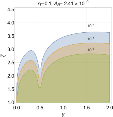
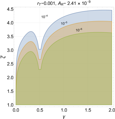
Figure 1: The critical density bounds during the quasi-de Sitter stage of expansion are illustrated in the $(\gamma,\,\overline{\zeta})$ plane. The difference between the left and right plots comes from a different value of the tensor to scalar ratio $r_{T}$ entering the estimate of $(H/M_{P})$

With the same notations used in Eq. (4.13) and (4.14) the hyperelectric spectra are instead given by:

$$P_{E}(k,\tau) = a^{4}H^{4}\,D(\gamma+1/2)\,Q_{E}(\overline{\zeta},\gamma)\,\biggl{(}\frac{k}{aH}\biggr{)}^{4-2\gamma},$$ (4.17)

$$P^{(G)}_{E}(k,\tau) = a^{4}H^{4}\,D(\gamma+1/2)\,Q^{(G)}_{E}(\overline{\zeta},\gamma)\,\biggl{(}\frac{k}{aH}\biggr{)}^{4-2\gamma},$$ (4.18)

where $D(x)$ has been already introduced in Eq. (4.15) while $Q_{E}(\overline{\zeta},\gamma)$ and $Q^{(G)}_{E}(\overline{\zeta},\gamma)$ are defined as:

$$Q_{E}(\overline{\zeta},\gamma)=\frac{1}{2}\biggl{[}\frac{e^{-\pi\overline{\zeta}}\,\Gamma^{2}(\gamma)}{\bigl{|}\Gamma(\gamma-i\overline{\zeta})\bigr{|}^{2}}+\frac{e^{\pi\overline{\zeta}}\,\Gamma^{2}(\gamma)}{\bigl{|}\Gamma(\gamma+i\overline{\zeta})\bigr{|}^{2}}\biggr{]},\qquad Q_{E}^{(G)}(\overline{\zeta},\gamma)=\frac{1}{2}\biggl{[}\frac{e^{-\pi\overline{\zeta}}\,\Gamma^{2}(\gamma)}{\bigl{|}\Gamma(\gamma-i\overline{\zeta})\bigr{|}^{2}}-\frac{e^{\pi\overline{\zeta}}\,\Gamma^{2}(\gamma)}{\bigl{|}\Gamma(\gamma+i\overline{\zeta})\bigr{|}^{2}}\biggr{]}.$$ (4.19)

Since $\overline{\zeta}=\lambda_{0}\gamma$ (and, as required in Eq. (4.3), $\gamma>0$) the limits for $\overline{\zeta}\to 0$ of Eqs. (4.16) and (4.19) correspond to the situation where the anomalous interactions are absent (i.e. $\lambda_{0}\to 0$):

$$\lim_{\overline{\zeta}\to 0}Q_{X}(\overline{\zeta},\gamma)=1,\qquad\lim_{\overline{\zeta}\to 0}Q^{(G)}_{X}(\overline{\zeta},\gamma)=0,\qquad\mathrm{for}\quad X=E,\,\,B.$$ (4.20)

When the relevant wavelengths exceed the effective horizon associated with the evolution of the gauge coupling the ratio of the gyrotropic spectrum to its non-gyrotropic counterpart assumes a particularly simple form:

$$\lim_{(-k\tau)\ll 1}\frac{P^{(G)}_{B}(k,\tau)}{P_{B}(k,\tau)}=\lim_{(-k\tau)\ll 1}\frac{P^{(G)}_{E}(k,\tau)}{P_{E}(k,\tau)}=-\tanh{\pi\,\overline{\zeta}},$$ (4.21)

implying that for $\overline{\zeta}\gg 1$ the two components are of the same order while in the limit $\pi\overline{\zeta}<1$ the gyrotropic contribution is always subleading.

4.3 Bound on the strength of anomalous interactions

The result of Eq. (4.21) suggests that the limits of Eqs. (4.13)–(4.14) and (4.17)–(4.18) for $\overline{\zeta}\to 0$ exactly coincide with the results valid in the absence of anomalous interactions (see e.g. [41] and references therein):

$$\lim_{\overline{\zeta}\to 0}\,\,P_{B}(k,\tau) = a^{4}H^{4}\,D(|\gamma-1/2|)\,\biggl{(}\frac{k}{aH}\biggr{)}^{5-|2\gamma-1|},$$ (4.22)

$$\lim_{\overline{\zeta}\to 0}\,\,P_{E}(k,\tau) = a^{4}H^{4}\,D(\gamma+1/2)\,\biggl{(}\frac{k}{aH}\biggr{)}^{4-2\gamma},$$ (4.23)

$$\lim_{\overline{\zeta}\to 0}\,\,P^{(G)}_{B}(k,\tau) = \lim_{\overline{\zeta}\to 0}\,\,P^{(G)}_{E}(k,\tau)=0.$$ (4.24)

This observation is relevant for the derivation of the general bounds on the parameter space of the model: since we want to make sure that the obtained constraints will have general validity we shall first consider the limit $\overline{\zeta}\to 0$. Equations (4.22) and (4.23) assume a different form in two complementary situations, namely the cases $\gamma>1/2$ and $0<\gamma<1/2$. If $\gamma>1/2$ the hypermagnetic spectrum $P_{B}(k,\tau)$ is scale-invariant for $\gamma=3$; but for this value $\gamma$ the hyperelectric spectrum $P_{E}(k,\tau)$ diverges in the limit $(-k\tau)\ll 1$. When $\gamma=2$ the hyperelectric spectrum is scale-invariant but the corresponding hypermagnetic spectrum is sharply increasing with $|k\,\tau|$. If $0<\gamma<1/2$ both the hyperelectric and the hypermagnetic spectra are increasing. We therefore conclude that the physical range of $\gamma$ pinned down by the explicit expressions (4.22)–(4.23) is given by $0<\gamma\leq 2$.

The constraints on the strength of the anomalous interactions in the $(\gamma,\overline{\zeta})$ will now follow from the bounds on the spectral energy density during the quasi-de Sitter stage of expansion. Thanks to Eqs. (4.13)–(4.14) and (4.17)–(4.18) the general form of the spectral energy density given in Eq. (3.11) becomes

$$\Omega_{Y}(k,\tau)=\frac{2}{3}\biggl{(}\frac{H}{M_{P}}\biggr{)}^{2}\biggl{[}D(|\gamma-1/2|)Q_{B}(\overline{\zeta},\gamma)\biggl{(}\frac{k}{aH}\biggr{)}^{5-|2\gamma-1|}+D(\gamma+1/2)Q_{E}(\overline{\zeta},\gamma)\biggl{(}\frac{k}{aH}\biggr{)}^{4-2\gamma}\biggr{]},$$ (4.25)

and must always remain much smaller than $1$ during the whole quasi-de Sitter stage of expansion. Using Eqs. (4.22)–(4.23) the limit of Eq. (4.25) for $\overline{\zeta}\ll 1$ is:

$$\Omega_{Y}(k,\tau)=\frac{2}{3}\biggl{(}\frac{H}{M_{P}}\biggr{)}^{2}\biggl{[}D(|\gamma-1/2|)\biggl{(}\frac{k}{aH}\biggr{)}^{5-|2\gamma-1|}+D(\gamma+1/2)\biggl{(}\frac{k}{aH}\biggr{)}^{4-2\gamma}\biggr{]}.$$ (4.26)

From Eq. (4.26) we then conclude that for $\overline{\zeta}\ll 1$ the spectral energy density is subcritical (i.e. $\Omega_{Y}(k,\tau)\ll 1$) provided $\gamma\leq 2$. If $\overline{\zeta}\geq 1$ we cannot avoid a more numerical discussion which is summarized in Fig. 1 where the two dimensional contours in the plane $(\gamma,\,\overline{\zeta})$ are illustrated in various cases. For the sake of illustration in Fig. 1 the regions with the different shadings correspond to the maximal values of $\Omega_{Y}(k,\tau)$ indicated in the figure (i.e. $10^{-6}$, $10^{-5}$ and $10^{-4}$ from bottom to top). Note finally that in Fig. 1 we assumed the validity of the consistency relations stipulating that $\epsilon=r_{T}/16$ where $r_{T}$ denotes the tensor to scalar ratio. We therefore conclude that as long as $\overline{\zeta}={\mathcal{O}}(\gamma)$ the spectral energy density is subcritical.

4.4 Late time evolution of the mode functions

For $\tau\geq-\tau_{1}$ the rate of variation of $\sqrt{\lambda}$ and the other relevant variables follow from Eq. (4.2):

$${\mathcal{F}} = -\frac{\delta}{y(\tau)},\qquad y(\tau)=\tau+\tau_{1}[q(\gamma,\delta)+1],\qquad q(\gamma,\delta)=\delta/\gamma$$ (4.27)

$$\xi = i\overline{\xi},\qquad\overline{\xi}=\lambda_{0}\delta,\qquad w=2i\,k\,y,\qquad\nu=(\delta+1/2).$$ (4.28)

Given that $\xi$ is also a purely imaginary quantity, $\overline{\xi}$ has the same meaning of $\overline{\zeta}$ [see Eq. (4.6)]. Furthermore since $\delta\ll\gamma$ [see Eq. (4.3)] we will also have that $\overline{\xi}\ll\overline{\zeta}$. The relation of $y(\tau)$ and $w(\tau)$ to the conformal time coordinate is always linear but it also contains a constant piece (multiplied by $q(\gamma,\delta)=\delta/\gamma$) which is relevant for the accurate continuity of the various expressions. With these precisions, for $\tau\geq-\tau_{1}$ the canonical forms of the Whittaker’s equations for the $L$ and $R$ polarizations are:

$$\frac{d^{2}f_{k,\,L}}{dw^{2}}+\biggl{[}-\frac{1}{4}-\frac{\xi}{w}-\frac{\nu^{2}-1/4}{w^{2}}\biggr{]}f_{k,\,L}=0,\qquad\frac{d^{2}f_{k,\,R}}{dw^{2}}+\biggl{[}-\frac{1}{4}+\frac{\xi}{w}-\frac{\nu^{2}-1/4}{w^{2}}\biggr{]}f_{k,\,R}=0,$$ (4.29)

$$g_{k,\,L}=2\,i\,k\,\biggl{[}\frac{df_{k,\,L}}{dw}-\frac{\delta}{w}f_{k,\,L}\biggr{]},\qquad g_{k,\,R}=2\,i\,k\,\biggl{[}\frac{df_{k,\,R}}{dw}-\frac{\delta}{w}f_{k,\,R}\biggr{]}.$$ (4.30)

The late-time form of the mode functions now follows from the continuity of the background and of the geometry. For the present ends it is particularly convenient to express $f_{k\,X}(\tau)$ and $g_{k\,X}(\tau)$ for $\tau>-\tau_{1}$ in terms of the corresponding mode functions computed for $\tau\leq-\tau_{1}$:

$$f_{k\,X}(\tau) = A_{f\,f}^{(X)}(w_{1},\,w,\,\delta)\overline{f}_{k,\,X}+A_{f\,g}^{(X)}(w_{1},\,w,\,\delta)\,\frac{\overline{g}_{k,\,X}}{k},$$ (4.31)

$$g_{k\,X}(\tau) = A_{f\,f}^{(X)}(w_{1},\,w,\,\delta)k\,\overline{f}_{k,\,X}+A_{g\,g}^{(X)}(w_{1},\,w,\,\delta)\,\overline{g}_{k,\,X},$$ (4.32)

where $X=L,\,R$ since Eqs. (4.31)–(4.32) hold independently for the left- and for the right-movers. Note that the functions $\overline{f}_{k,\,X}$ and $\overline{g}_{k,\,X}$ are just the mode functions valid for $\tau\leq-\tau_{1}$ evaluated for $\tau=-\tau_{1}$, i.e.

$$\overline{f}_{k,\,X}\equiv f^{(inf)}_{k,\,X}(-\tau_{1}),\qquad\mathrm{and}\qquad\overline{g}_{k,\,X}\equiv g^{(inf)}_{k,\,X}(-\tau_{1}),\qquad\mathrm{for}\quad X=R,\,L.$$ (4.33)

The variable $w_{1}$ appearing in Eqs. (4.31)–(4.32) is, by definition, $w1=w(-\tau_{1})$. Hence, from the definition of $y(\tau)$ given in Eq. (4.27) we will also have that $w_{1}=2i\,k\,\tau_{1}q$. The various terms appearing in Eqs. (4.31)–(4.32) can also be ordered in an appropriate mixing matrix:

$${\mathcal{M}}^{(X)}(w_{1},\,w,\,\delta)=\left(\matrix{A^{(X)}_{f\,f}(w_{1},\,w,\,\delta)&A^{(X)}_{f\,g}(w_{1},\,w,\,\delta)&\cr A^{(X)}_{g\,f}(w_{1},\,w,\,\delta)&A^{(X)}_{g\,g}(w_{1},\,w,\,\delta)&\cr}\right).$$ (4.34)

Since the Wronskian normalization has been fixed in the limit $\tau\to-\infty$ (and it is preserved by the continuity and differentiability of the evolution) the determinant of ${\mathcal{M}}^{(X)}(w_{1},\,w,\,\delta)$ must be equal to $1$:

$$A_{f\,f}^{(X)}(w_{1},\,w,\,\delta)A^{(X)}_{g\,g}(w_{1},\,w,\,\delta)-A^{(X)}_{f\,g}(w_{1},\,w,\,\delta)A^{(X)}_{g\,f}(w_{1},\,w,\,\delta)=1.$$ (4.35)

The explicit forms of the various entries of the matrix (4.34) are determined from the linearly independent solutions of Eqs. (4.29) and (4.30) listed in appendix B [i.e. Eqs. (B.2) and (B.3)–(B.4)]:

$$A^{(L)}_{f\,f}(w_{1},w,\delta) = -\frac{e^{\pi\overline{\xi}}}{2w_{1}}\biggl{\{}(w_{1}-2\delta-2\xi)W_{-\xi,\nu}\left(-w_{1}\right)W_{\xi,\nu}(w)+2W_{1-\xi,\nu}(-w_{1})W_{\xi,\nu}(w)$$ (4.36)

$$+ W_{-\xi,\nu}(-w)\biggl{[}\left(2\delta-2\xi+w_{1}\right)W_{\xi,\nu}\left(w_{1}\right)-2W_{\xi+1,\nu}(w_{1})\biggr{]}\biggr{\}},$$

$$A^{(L)}_{f\,g}(w_{1},w,\delta) = \frac{i}{2}e^{\pi\overline{\xi}}\biggl{[}W_{-\xi,\nu}\left(-w_{1}\right)W_{\xi,\nu}(w)-W_{-\xi,\nu}(-w)W_{\xi,\nu}\left(w_{1}\right)\biggr{]},$$ (4.37)

$$A^{(L)}_{g\,f}(w_{1},w,\delta) = \frac{i\,e^{\pi\overline{\xi}}}{2w\,w_{1}}\biggl{\{}\biggl{[}\left(2\delta+2\xi-w_{1}\right)W_{-\xi,\nu}(-w_{1})-2W_{1-\xi,\nu}(-w_{1})\biggr{]}\biggl{[}(2\delta-2\xi+w)W_{\xi,\nu}(w)$$ (4.38)

$$- 2W_{\xi+1,\nu}(w)\biggr{]}-\biggl{[}(2\delta+2\xi-w)W_{-\xi,\nu}(-w)-2W_{1-\xi,\nu}(-w)\biggr{]}\biggl{[}\left(2\delta-2\xi+w_{1}\right)W_{\xi,\nu}(w_{1})$$

$$- 2W_{\xi+1,\nu}(w_{1})\biggr{]}\biggr{\}},$$

$$A^{(L)}_{g\,g}(w_{1},w,\delta) = -\frac{e^{\pi\overline{\xi}}}{2w}\biggl{\{}W_{\xi,\nu}\left(w_{1}\right)\biggl{[}(w-2\delta-2\xi)W_{-\xi,\nu}(-w)+2W_{1-\xi,\nu}(-w)\biggr{]}$$ (4.39)

$$+ W_{-\xi,\nu}\left(-w_{1}\right)\biggl{[}(2\delta-2\xi+w)W_{\xi,\nu}(w)-2W_{\xi+1,\nu}(w)\biggr{]}\biggr{\}}.$$

In Eqs. (4.36)–(4.37) and (4.38)–(4.39) the dependence upon $\delta$ appears, implicitly, in $\nu(\delta)$ [because of Eq. (4.28)] and also in $\xi=i\overline{\xi}$ [since $\overline{\xi}=\lambda_{0}\delta$]. The entries of the companion matrix valid for the $R$-polarization (i.e. ${\mathcal{M}}^{(R)}(w_{1},\,w,\,\delta)$) have a form similar to ${\mathcal{M}}^{(L)}(w_{1},\,w,\,\delta)$ and they are obtained from the expressions reported in appendix B (see, in particular, Eqs. (B.5) and (B.6)–(B.7)). Just to state the rule of thumb we now compare the result of Eq. (4.37) with the analog expression of $A^{(R)}_{f\,g}(w_{1},w,\delta)$:

$$A^{(R)}_{f\,g}(w_{1},w,\delta)=\frac{i}{2}e^{-\pi\overline{\xi}}\biggl{[}W_{-\xi,\nu}\left(w_{1}\right)W_{\xi,\nu}(-w)-W_{-\xi,\nu}(w)W_{\xi,\nu}\left(-w_{1}\right)\biggr{]}.$$ (4.40)

Therefore, to obtain the explicit form of ${\mathcal{M}}^{(R)}(w_{1},\,w,\,\delta)$ once the entries of ${\mathcal{M}}^{(L)}(w_{1},\,w,\,\delta)$ are known it is sufficient to flip the signs of $w_{1}$ and $w$ in Eqs. (4.36)–(4.37) and (4.38)–(4.39) and to flip the sign of $\overline{\xi}$ in the normalization appearing in the different entries. It is finally interesting to analyze the Hankel limit of the mixing matrices, namely the limit $\overline{\xi}\to 0$ (see also Eqs. (A.6)–(A.8) and discussion therein). Since $\overline{\xi}=\lambda_{0}\,\delta$, the limit $\overline{\xi}\to 0$ can be realized in two complementary (but physically distinct) cases. The first interesting limit is $\lambda_{0}\to 0$ (while $\delta\neq 0$); in this case the anomalous contribution vanishes but the gauge coupling is still increasing for $\tau\geq-\tau_{1}$. In this case the matrix elements of ${\mathcal{M}}^{(R)}(w_{1},\,w,\,\delta)$ and of ${\mathcal{M}}^{(L)}(w_{1},\,w,\,\delta)$ coincide and are given by:

$$\lim_{\lambda_{0}\to 0}\,{\mathcal{M}}^{(R)}(w_{1},\,w,\,\delta)=\lim_{\lambda_{0}\to 0}\,{\mathcal{M}}^{(L)}(w_{1},\,w,\,\delta)=\left(\matrix{A_{f\,f}(\tau_{1},\,\tau,\,\delta)&A_{f\,g}(\tau_{1},\,\tau,\,\delta)&\cr A_{g\,f}(\tau_{1},\,\tau,\,\delta)&A_{g\,g}(\tau_{1},\,\tau,\,\delta)&\cr}\right).$$ (4.41)

where the explicit expressions of the various entries appearing in the common limit of Eq. (4.41) are:

$$A_{f\,f}(k,\tau,\tau_{1}) = \frac{\pi}{2}\sqrt{qx_{1}}\sqrt{ky}\biggl{[}Y_{\nu-1}(qx_{1})J_{\nu}(ky)-J_{\nu-1}(qx_{1})Y_{\nu}(ky)\biggr{]},$$

$$A_{f\,g}(k,\tau,\tau_{1}) = \frac{\pi}{2}\sqrt{qx_{1}}\sqrt{ky}\biggl{[}J_{\nu}(qx_{1})Y_{\nu}(ky)-Y_{\nu}(qx_{1})J_{\nu}(ky)\biggr{]},$$

$$A_{g\,f}(k,\tau,\tau_{1}) = \frac{\pi}{2}\sqrt{qx_{1}}\sqrt{ky}\biggl{[}Y_{\nu-1}(qx_{1})J_{\nu-1}(ky)-J_{\nu-1}(qx_{1})Y_{\nu-1}(ky)\biggr{]},$$

$$A_{g\,g}(k,\tau,\tau_{1}) = \frac{\pi}{2}\sqrt{qx_{1}}\sqrt{ky}\biggl{[}J_{\nu}(qx_{1})Y_{\nu-1}(ky)-Y_{\nu}(qx_{1})J_{\nu-1}(ky)\biggr{]},$$ (4.42)

where $x_{1}=k\tau_{1}$ while $y$ has the same definition given before (see prior to Eq. (4.28)); note that the matrix elements (4.42) still obey Eq. (4.41).

The second way in which the limit $\overline{\xi}\ll 1$ can be physically realized suggests that $\delta\to 0$ (while $\lambda_{0}\neq 0$). In this case the anomalous contributions remain for $\tau\geq-\tau_{1}$ but the gauge coupling flattens out, at least approximately. By keeping fixed $x=k\tau$ and $x_{1}=k\tau_{1}$ the common limit of ${\mathcal{M}}^{(L)}(w_{1},\,w,\,\delta)$ and of ${\mathcal{M}}^{(R)}(w_{1},\,w,\,\delta)$ is now even simpler:

$$A_{f\,f}(k,\tau,\tau_{1})=\cos{[k(\tau+\tau_{1})]}+{\mathcal{O}}(\delta),\qquad A_{f\,g}(k,\tau,\tau_{1})=\sin{[k(\tau+\tau_{1})]}+{\mathcal{O}}(\delta),$$

$$A_{g\,f}(k,\tau,\tau_{1})=-\sin{[k(\tau+\tau_{1})]}+{\mathcal{O}}(\delta),\qquad A_{g\,f}(k,\tau,\tau_{1})=\cos{[k(\tau+\tau_{1})]}+{\mathcal{O}}(\delta).$$ (4.43)

The finiteness of the result (4.43) demonstrates that the continuity of the mode functions is an essential requirement for the correctness of the asymptotic results.

4.5 Late-time hypermagnetic and hyperelectric power spectra

The matrices ${\mathcal{M}}^{(X)}(w_{1},\,w,\,\delta)$ introduced in Eq. (4.34) effectively mix the hypermagnetic and the hyperelectric mode functions computed at the end of inflation. There is therefore no reason to expect that the late-time hypermagnetic power spectra will have to coincide (either exactly or approximately) with the hypermagnetic spectra at the end of inflation, as it is sometimes assumed. In their full form the late-time spectra for $\tau\geq-\tau_{1}$ will be given by:

$$P_{B}(k,\tau) = \frac{k^{5}}{4\pi^{2}}\sum_{X=L,\,R}\biggl{|}A_{f\,f}^{(X)}(w_{1},\,w,\,\delta)\,\,\overline{f}_{k,\,X}+A_{f\,g}^{(X)}(w_{1},\,w,\,\delta)\,\,\frac{\overline{g}_{k,\,X}}{k}\biggr{|}^{2},$$ (4.44)

$$P_{E}(k,\tau) = \frac{k^{3}}{4\pi^{2}}\,\sum_{X=L,\,R}\biggl{|}A_{g\,f}^{(X)}(w_{1},\,w,\,\delta)\,k\,\overline{f}_{k,\,X}+A_{g\,g}^{(X)}(w_{1},\,w,\,\delta)\,\,\overline{g}_{k,\,X}\,\,\biggr{|}^{2}.$$ (4.45)

Since the hyperelectric and hypermagnetic mode functions at the end of inflation are not of the same order, also the contributions entering Eqs. (4.44)–(4.45) are not all comparable. For instance in the case of the hypermagnetic power spectrum of Eq. (4.44) the first term inside the square modulus dominates against the second term:

$$\biggl{|}A^{(X)}_{f\,g}(w_{1},w,\delta)\,\frac{\overline{g}_{k,\,X}}{k}\biggr{|}\gg\biggl{|}A_{f\,f}^{(X)}(w_{1},w,\delta)\,\overline{f}_{k,\,X}\biggr{|},\qquad\mathrm{for}\quad X=R,\,\,L.$$ (4.46)

The simplest way of proving the inequality (4.46) is to consider the physically relevant regime where the modes are still larger than the effective horizon for $\tau\geq-\tau_{1}$ (i.e. $k\tau_{1}<k\tau\ll 1$) while the gauge coupling either flattens out or even freezes; according to Eq. (4.3) this regime corresponds to the situation where

$$0<\delta\ll\gamma\qquad\Rightarrow 0<\delta<1/2\qquad\Rightarrow\nu=1/2-\delta.$$ (4.47)

Using Eq. (4.47) in the limit $k\tau_{1}<k\tau\ll 1$ together with the explicit expressions of the mode functions we obtain that Eq. (4.46) is verified in spite of the value of $\lambda_{0}$: this happens since for $\delta\to 0$ the limit $\overline{\xi}\to 0$ is verified for any $\lambda_{0}={\mathcal{O}}(1)$. Equation (4.46) is complemented by the analog inequality (actually motivated by duality as we shall see at the end of section 5) valid in the hyperelectric case, namely:

$$\biggl{|}A_{g\,f}^{(X)}(w_{1},\,w,\,\delta)\,k\,\overline{f}_{k,\,X}\biggr{|}\ll\biggl{|}A_{g\,g}^{(X)}(w_{1},\,w,\,\delta)\overline{g}_{k,\,X}\biggr{|},\qquad\mathrm{for}\quad X=R,\,\,L.$$ (4.48)

If the variables $w$ and $w_{1}$ are traded for $x=k\tau$ and for $x_{1}=k\tau_{1}$ the general expression of the hypermagnetic and hyperelectric power spectra can be written as:

$$P_{B}(k,\tau) = \frac{k^{5}}{2\pi^{2}}\biggl{[}\biggl{|}A^{(L)}_{f\,g}(x_{1},\,x,\delta)\,\frac{\overline{g}_{k,\,L}}{k}\biggr{|}^{2}+\biggl{|}A^{(R)}_{f\,g}(x_{1},\,x,\delta)\,\frac{\overline{g}_{k,\,R}}{k}\biggr{|}^{2}\biggr{]},$$ (4.49)

$$P_{E}(k,\tau) = \frac{k^{3}}{2\pi^{2}}\biggl{[}\biggl{|}A^{(L)}_{g\,g}(x_{1},\,x,\delta)\,\overline{g}_{k,\,L}\biggr{|}^{2}+\biggl{|}A^{(R)}_{f\,g}(x_{1},\,x,\delta)\,\overline{g}_{k,\,R}\biggr{|}^{2}\biggr{]}.$$ (4.50)

Equations (4.49) and (4.50) are actually very interesting since they show that, when the gauge coupling first increases and then flattens out, the late-time power spectra are determined by the hyperelectric power spectra at the end of inflation. For a fixed value of $x_{1}$ and $x$ we have that $A^{(L)}_{f\,g}(x_{1},\,x,\delta)$ and $A^{(R)}_{f\,g}(x_{1},\,x,\delta)$ differ at most by terms ${\mathcal{O}}(\delta)$ in the limit $\delta\to 0$

$$\lim_{\delta\ll 1}\biggl{[}A^{(R)}_{f\,g}(x_{1},\,x,\delta)-A^{(L)}_{f\,g}(x_{1},\,x,\delta)\biggr{]}={\mathcal{O}}(\delta).$$ (4.51)

Since the reasonable values of $\delta$ do not exceed ${\mathcal{O}}(0.1)$, the power spectra can be estimated, in this range, as:

$$P_{B}(k,\tau) = a_{1}^{4}\,H_{1}^{4}\,D(\gamma+1/2)\,x_{1}^{4-2\gamma}\,F_{B}(x_{1},x,\delta,\overline{\zeta},\gamma),$$

$$F_{B}(x_{1},x,\delta,\overline{\zeta},\gamma) = \biggl{|}A^{(X)}_{f\,g}(x_{1},\,x,\delta)\biggr{|}^{2}Q_{E}(\overline{\zeta},\gamma)=[\sin{(x+x_{1})}+{\mathcal{O}}(\delta)]^{2}\,Q_{E}(\overline{\zeta},\gamma).$$ (4.52)

The limit $\delta\to 0$ can be explicitly compared with the estimates obtained when, for instance, $\delta={\mathcal{O}}(10^{-2})$ and this is what will also be specifically illustrated in section 6. With the same approach leading to Eq. (4.52) the hyperelectric power spectrum becomes

$$P_{E}(k,\tau) = a_{1}^{4}\,H_{1}^{4}\,D(\gamma+1/2)\,x_{1}^{4-2\gamma}\,F_{E}(x_{1},x,\delta,\overline{\zeta},\gamma),$$

$$F_{E}(x_{1},x,\delta,\overline{\zeta},\gamma) = \biggl{|}A^{(X)}_{g\,g}(x_{1},\,x,\delta)\biggr{|}^{2}Q_{E}(\overline{\zeta},\gamma)=[\cos{(x+x_{1})}+{\mathcal{O}}(\delta)]^{2}\,Q_{E}(\overline{\zeta},\gamma).$$ (4.53)

Equations (4.52)–(4.53) are therefore a consequence of Eqs. (4.49)–(4.50) and they explicitly show that the late-time hypermagnetic spectra are determined by their hyperelecric counterpart at the end of the inflationary phase; this is ultimately the reason why $Q_{E}(\overline{\zeta},\gamma)$ appears in Eq. (4.52). The amplitudes of the two spectra are however quite different: while $P_{B}(k,\tau)$ exhibits standing oscillations going as $\sin^{2}{(x+x_{1})}$ the hyperelectric oscillations go instead as $P_{E}(k,\tau)\propto\cos^{2}{(x+x_{1})}$. This means that while $P_{B}(k,\tau)\ll P_{E}(k,\tau)$ when $k\tau\ll 1$, as the relevant modes cross the Hubble radius $P_{B}(k,\tau_{k})\simeq P_{E}(k,\tau_{k})$ where $\tau_{k}$ is defined by the condition $k\,\tau_{k}={\mathcal{O}}(1)$. The same strategy employed to estimate the power spectra can be used with the corresponding gyrotropies. We shall omit this discussion for the sake of conciseness and mention the final results for $P_{B}^{(G)}(k,\tau)$ and $P_{E}^{(G)}(k,\tau)$:

$$P_{B}^{(G)}(k,\tau) = a_{1}^{4}\,H_{1}^{4}\,D(\gamma+1/2)\,x_{1}^{4-2\gamma}\,Q^{(G)}_{B}(\overline{\zeta},\gamma)\,\sin^{2}{(x+x_{1})},$$ (4.54)

$$P_{E}^{(G)}(k,\tau) = a_{1}^{4}\,H_{1}^{4}\,D(\gamma+1/2)\,x_{1}^{4-2\gamma}\,Q^{(G)}_{E}(\overline{\zeta},\gamma)\,\cos^{2}{(x+x_{1})}.$$ (4.55)

We note in passing that the standing waves appearing in Eqs. (4.54) and (4.55) are the gauge analog of the Sakharov oscillations [51, 52].

5 The case of decreasing gauge coupling and the related bounds

While in section 4 we examined a phase of increasing gauge coupling, in this section we shall examine the dual situation where the evolution of $\sqrt{\lambda}$ is given by:

$$\sqrt{\lambda} = \sqrt{\lambda_{1}}\biggl{(}-\frac{\tau}{\tau_{1}}\biggr{)}^{-\widetilde{\,\gamma\,}},\qquad\tau<-\tau_{1},$$ (5.1)

$$\sqrt{\lambda} = \sqrt{\lambda_{1}}\biggl{[}\frac{\widetilde{\,\gamma\,}}{\widetilde{\,\delta\,}}\biggl{(}\frac{\tau}{\tau_{1}}+1\biggr{)}+1\biggr{]}^{\widetilde{\,\delta\,}},\qquad\tau\geq-\tau_{1}.$$ (5.2)

If we compare Eqs. (5.1)–(5.2) with Eqs. (4.1)–(4.2) we see that the quantities with tilde will always correspond to the situation where the gauge coupling decreases. This notation simplifies the comparison of the power spectra in the dual cases, as we shall see at the end of this section. The physical region of the parameters $\widetilde{\gamma}$ and $\widetilde{\delta}$ appearing in Eqs. (5.1)–(5.2) is:

$$\widetilde{\,\gamma\,}>0,\qquad\widetilde{\,\delta\,}\geq 0,\qquad\mathrm{and}\qquad 0<\widetilde{\,\delta\,}\ll\widetilde{\,\gamma\,}.$$ (5.3)

We want to stress that dual profiles of Eqs. (4.1)–(4.2) and (5.1)–(5.2) are not physically equivalent. Equation (5.1) implies that at the onset of the inflationary phase the gauge coupling may be very large:

$$\sqrt{\lambda_{i}}=\sqrt{\lambda_{1}}\biggl{(}\frac{a_{i}}{a_{f}}\biggr{)}^{\widetilde{\,\gamma\,}}\ll 1\qquad\qquad\Rightarrow\qquad\qquad e(\tau_{i})=\frac{\sqrt{4\pi}}{\sqrt{\lambda_{i}}}\gg 1,$$ (5.4)

where, by definition, $\lambda_{i}=\lambda(-\tau_{i})$. Equation (5.4) implies that the evolution of the gauge coupling starts from a non-perturbative regime unless $\sqrt{\lambda_{1}}$ is extremely large: only in this way we could possibly have $\sqrt{\lambda_{i}}={\mathcal{O}}(1)$. Whenever $\sqrt{\lambda_{1}}\gg 1$ the gauge coupling will be extremely minute at the end of inflation and this is at odds with the fact that during the decelerated stage of expansion we would like to have $e^{2}={\mathcal{O}}(10^{-2})$ but not much smaller. Furthermore, as we shall discuss in section 6, the physical power spectra are suppressed as $\lambda_{1}^{-1}$ and this will make their contribution marginal for the phenomenological implications. A possibility suggested previously has been that the $\sqrt{\lambda}$ increases during inflation, decreases sharply during reheating, and then flattens out again. This suggestion has been originally put forward in Refs. [53] (see also [54]) and it would imply a sudden decrease of $\sqrt{\lambda}$ in an extremely short time. This hopeful possibility will not be necessary in the present context.

5.1 Mode functions and their normalization during the quasi-de Sitter stage

During the inflationary phase the explicit expressions of the evolution of the mode functions are given by Eq. (A.3) (see also the related discussion in the appendix A). Equations (2.18) and (2.19) become:

$$\frac{d^{2}f_{k,\,L}}{dz^{2}}+\biggl{[}-\frac{1}{4}-\frac{\eta}{z}-\frac{\widetilde{\,\mu\,}^{2}-1/4}{z^{2}}\biggr{]}f_{k,\,L}=0,\qquad\frac{d^{2}f_{k,\,R}}{dz^{2}}+\biggl{[}-\frac{1}{4}+\frac{\eta}{z}-\frac{\widetilde{\,\mu\,}^{2}-1/4}{z^{2}}\biggr{]}f_{k,\,R}=0,$$ (5.5)

where the variables appearing in Eq. (5.5) are now defined as:

$$z=2\,i\,k\,\tau,\qquad\widetilde{\,\mu\,}=\widetilde{\,\gamma\,}+1/2,\qquad\eta=i\,\overline{\eta},\qquad\overline{\eta}=\lambda_{0}\,\widetilde{\,\gamma\,}.$$ (5.6)

Equations (5.5)–(5.6) are written in the canonical Whittaker form (see also Eq. (A.5)). By comparing Eqs. (5.5)–(5.6) with Eqs. (4.5)–(4.6) it is useful to stress the differences but also the possible symmetries especially for what concerns the sign of the anomalous contributions. From Eqs. (5.5)–(5.6) the solutions for $f_{k\,L}(z)$ and $f_{k\,R}(z)$ are:

$$f_{k\,L}(z)=\widetilde{\,C\,}_{L}(k,\overline{\eta})\,W_{-\eta,\,\widetilde{\mu}}(z),\qquad\qquad f_{k\,R}(z)=\widetilde{\,C\,}_{R}(k,\overline{\eta})\,W_{\eta,\,\widetilde{\mu}}(z),$$ (5.7)

where the factors $\widetilde{\,C\,}_{R}(k,\overline{\eta})$ and $\widetilde{\,C\,}_{L}(k,\overline{\eta})$ are fixed from the Wronskian normalization condition (2.17) in the limit $\tau\ll-\tau_{1}$:

$$\widetilde{\,C\,}_{R}(k,\overline{\eta})=\frac{e^{-i\pi/4-\pi\overline{\eta}/2}}{\sqrt{2k}},\qquad\qquad\widetilde{\,C\,}_{L}(k,\overline{\eta})=\frac{e^{i\pi/4+\pi\overline{\eta}/2}}{\sqrt{2k}}.$$ (5.8)

As before the results of appendix A can be used together with Eq. (5.7) so that the explicit form of the hyperelectric mode functions is:

$$g_{k\,R}(z)=2\,i\,k\,\widetilde{\,C\,}_{R}(k,\overline{\eta})\biggl{[}\frac{z+2(\widetilde{\gamma}-\eta)}{2z}W_{\eta,\,\widetilde{\mu}}(z)-\frac{W_{1+\eta,\,\widetilde{\mu}}(z)}{z}\biggr{]},$$ (5.9)

$$g_{k\,L}(z)=2\,i\,k\,\widetilde{\,C\,}_{L}(k,\overline{\eta})\biggl{[}\frac{z+2(\eta+\widetilde{\gamma})}{2z}W_{-\eta,\,\widetilde{\mu}}(z)-\frac{W_{1-\eta,\,\widetilde{\mu}}(z)}{z}\biggr{]}.$$ (5.10)

5.2 Hypermagnetic and hyperelectric power spectra during the quasi-de Sitter stage

After inserting the normalized solutions of Eqs. (5.7)–(5.8) into Eqs. (3.7)–(3.8) the explicit form of the hypermagnetic power spectra when the typical wavelengths are larger than the effective horizon is:

$$\widetilde{\,P\,}_{B}(k,\tau) = a^{4}\,H^{4}\,D(\widetilde{\,\gamma\,}+1/2)\,\biggl{(}\frac{k}{aH}\biggr{)}^{4-2\widetilde{\,\gamma\,}}\,\widetilde{\,Q\,}_{B}(\overline{\eta},\widetilde{\,\gamma\,}),$$ (5.11)

$$\widetilde{\,P\,}^{(G)}_{B}(k,\tau) = a^{4}\,H^{4}\,D(\widetilde{\,\gamma\,}+1/2)\,\biggl{(}\frac{k}{aH}\biggr{)}^{4-2\widetilde{\,\gamma\,}}\,\widetilde{\,Q\,}^{(G)}_{B}(\overline{\eta},\widetilde{\,\gamma\,}),$$ (5.12)

where $D(x)$ has been already defined in Eq. (4.15) and it has here exactly the same meaning in terms of the new argument; $\widetilde{\,Q\,}_{B}(\overline{\eta},\widetilde{\gamma})$ and $\widetilde{\,Q\,}^{(G)}_{B}(\overline{\eta},\widetilde{\gamma})$ are now given by:

$$\widetilde{\,Q\,}_{B}(\overline{\eta},\widetilde{\,\gamma\,})=\frac{1}{2}\biggl{[}\frac{e^{\pi\overline{\eta}}\,\,\Gamma^{2}(\widetilde{\,\gamma\,})}{\bigl{|}\Gamma(\widetilde{\,\gamma\,}-i\overline{\eta})\bigr{|}^{2}}+\frac{e^{-\pi\overline{\eta}}\,\,\Gamma^{2}(\widetilde{\,\gamma\,})}{\bigl{|}\Gamma(\widetilde{\,\gamma\,}+i\overline{\eta})\bigr{|}^{2}}\biggr{]},\qquad\widetilde{\,Q\,}^{(G)}_{B}(\overline{\eta},\widetilde{\,\gamma\,})=\frac{1}{2}\biggl{[}\frac{e^{\pi\overline{\eta}}\,\,\Gamma^{2}(\widetilde{\,\gamma\,})}{\bigl{|}\Gamma(\widetilde{\,\gamma\,}-i\overline{\eta})\bigr{|}^{2}}-\frac{e^{-\pi\overline{\eta}}\,\,\Gamma^{2}(\widetilde{\,\gamma\,})}{\bigl{|}\Gamma(\widetilde{\,\gamma\,}+i\overline{\eta})\bigr{|}^{2}}\biggr{]}.$$ (5.13)

The limit $\overline{\eta}\to 0$ mirrors the case $\overline{\zeta}\to 0$ discussed in Eq. (4.20):

$$\lim_{\overline{\eta}\to 0}\widetilde{\,Q\,}_{B}^{(G)}(\overline{\eta},\widetilde{\,\gamma\,})=1,\qquad\lim_{\overline{\eta}\to 0}\widetilde{\,Q\,}_{B}^{(G)}(\overline{\eta},\widetilde{\,\gamma\,})=0.$$ (5.14)

The asymptotic expression of the hyperelectric mode functions (see Eqs. (A.14)–(A.15)) is slightly more cumbersome and, to avoid confusions, the limits $\overline{\eta}\ll 1$ and $\overline{\eta}\gg 1$ will be separately discussed. If $\overline{\eta}\ll 1$ the hyperelectric spectra are

$$\widetilde{\,P\,}_{E}(k,\tau)=a^{4}\,H^{4}D(|\widetilde{\,\gamma\,}-1/2|)\,\biggl{(}\frac{k}{aH}\biggr{)}^{5-|2\widetilde{\,\gamma\,}-1|},\qquad\widetilde{\,P\,}_{E}^{(G)}(k,\tau)=0.$$ (5.15)

All in all in the limit $\overline{\eta}\to 0$ the gauge power spectra computed in the case of decreasing coupling are:

$$\lim_{\overline{\eta}\to 0}\,\,\widetilde{\,P\,}_{B}(k,\tau) = a^{4}H^{4}\,\,D(\widetilde{\,\gamma\,}+1/2)\,\biggl{(}\frac{k}{aH}\biggr{)}^{4-2\widetilde{\gamma}},$$ (5.16)

$$\lim_{\overline{\eta}\to 0}\,\,\widetilde{\,P\,}_{E}(k,\tau) = a^{4}H^{4}\,\,D(|\widetilde{\,\gamma\,}-1/2|)\,\biggl{(}\frac{k}{aH}\biggr{)}^{5-|2\widetilde{\gamma}-1|},$$ (5.17)

$$\lim_{\overline{\eta}\to 0}\,\,\widetilde{\,P\,}^{(G)}_{B}(k,\tau) = \lim_{\overline{\eta}\to 0}\,\,\widetilde{\,P\,}^{(G)}_{E}(k,\tau)=0.$$ (5.18)

In the opposite limit $\overline{\eta}\gg 1$ we have instead:

$$\widetilde{\,P\,}_{E}(k,\tau) = a^{4}\,H^{4}D(\widetilde{\,\gamma\,}+1/2)\,\biggl{(}\frac{k}{aH}\biggr{)}^{4-2\widetilde{\,\gamma\,}}\widetilde{\,Q\,}_{E}(\overline{\eta},\widetilde{\gamma}),$$ (5.19)

$$\widetilde{\,P\,}^{(G)}_{E}(k,\tau) = a^{4}\,H^{4}D(\widetilde{\,\gamma\,}+1/2)\,\biggl{(}\frac{k}{aH}\biggr{)}^{4-2\widetilde{\,\gamma\,}}\widetilde{\,Q\,}^{(G)}_{E}(\overline{\eta},\widetilde{\,\gamma\,}),$$ (5.20)

where $\widetilde{\,Q\,}_{E}(\overline{\eta},\widetilde{\,\gamma\,})$ and $\widetilde{\,Q\,}^{(G)}_{E}(\overline{\eta},\widetilde{\,\gamma\,})$ are now defined as:

$$\widetilde{\,Q\,}_{E}(\overline{\eta},\widetilde{\,\gamma\,})=\frac{\overline{\eta}^{2}}{2}\biggl{[}\frac{e^{\pi\overline{\eta}}\,\Gamma^{2}(\widetilde{\,\gamma\,})}{\bigl{|}\Gamma(\widetilde{\,\gamma\,}+i\overline{\eta})\bigr{|}^{2}}+\frac{e^{-\pi\overline{\eta}}\,\Gamma^{2}(\widetilde{\,\gamma\,})}{\bigl{|}\Gamma(\widetilde{\,\gamma\,}-i\overline{\eta})\bigr{|}^{2}}\biggr{]},\qquad\widetilde{\,Q\,}^{(G)}_{E}(\overline{\eta},\widetilde{\gamma})=\frac{\overline{\eta}^{2}}{2}\biggl{[}\frac{e^{\pi\overline{\eta}}\,\Gamma^{2}(\widetilde{\gamma})}{\bigl{|}\Gamma(\widetilde{\gamma}+i\overline{\eta})\bigr{|}^{2}}-\frac{e^{-\pi\overline{\eta}}\,\Gamma^{2}(\widetilde{\gamma})}{\bigl{|}\Gamma(\widetilde{\gamma}-i\overline{\eta})\bigr{|}^{2}}\biggr{]}.$$ (5.21)

When the relevant wavelengths exceed the effective horizon associated with the evolution of the gauge coupling the ratio of the gyrotropic spectrum to its non-gyrotropic counterpart is common to the hyperelectric and to the hypermagnetic case:

$$\lim_{(-k\tau)\ll 1}\frac{\widetilde{\,P\,}^{(G)}_{B}(k,\tau)}{\widetilde{\,P\,}_{B}(k,\tau)}=\lim_{(-k\tau)\ll 1}\frac{\widetilde{\,P\,}^{(G)}_{E}(k,\tau)}{\widetilde{\,P\,}_{E}(k,\tau)}=\tanh{\pi\,\overline{\eta}}.$$ (5.22)

If Eqs. (5.16)–(5.17) are inserted into Eq. (3.11) the spectral energy density is:

$$\Omega_{Y}(k,\tau)=\frac{2}{3}\biggl{(}\frac{H}{M_{P}}\biggr{)}^{2}\biggl{[}D(\widetilde{\gamma}+1/2)\biggl{(}\frac{k}{aH}\biggr{)}^{4-2\widetilde{\gamma}}+D(|\widetilde{\gamma}-1/2|)\biggl{(}\frac{k}{aH}\biggr{)}^{5-|2\widetilde{\gamma}-1|}\biggr{]},$$ (5.23)

and it is valid in the limit $\overline{\eta}\to 0$. In Eq. (5.23) the flat hypermagnetic spectrum corresponds to the case $\widetilde{\gamma}=2$ and the relevant region of the parameter space corresponds therefore to the interval $0<\widetilde{\gamma}\leq 2$ since for $\widetilde{\gamma}>2$ the spectral energy density $\Omega_{Y}(k,\tau)$ cannot be subcritical.

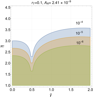
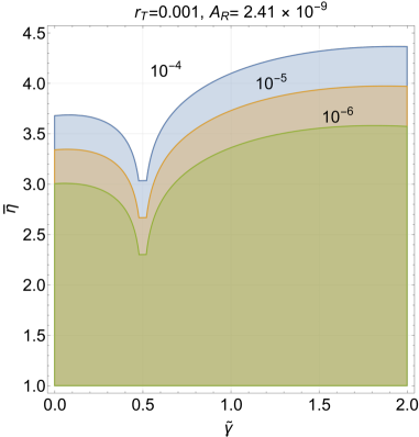
Figure 2: The critical density bounds during the quasi-de Sitter stage of expansion are illustrated in the $(\widetilde{\gamma},\,\overline{\eta})$ plane. As in difference between the left and right plots comes from a different value of the tensor to scalar ratio $r_{T}$ entering the estimate of $(H/M_{P})$.

If $\overline{\eta}\geq 1$ we can look directly at Fig. 2 where we illustrate the two dimensional contours in the plane $(\widetilde{\gamma},\,\overline{\eta})$. As in Fig. 1 the various shadings correspond to the values of $\Omega_{Y}(k,\tau)$ indicated in the plots (i.e. $10^{-6}$, $10^{-5}$ and $10^{-4}$ from bottom to top). In spite of the differences between Figs. 1 and 2 we can therefore conclude that for $0<\widetilde{\gamma}\leq 2$ and $\overline{\eta}>1$ the physical region of the parameters corresponds to $\overline{\eta}={\mathcal{O}}(\widetilde{\gamma})$.

5.3 Late-time mode functions and power spectra

For $\tau\geq-\tau_{1}$ the rate of variation of $\sqrt{\lambda}$ becomes, in this case ${\mathcal{F}}=\widetilde{\delta}/y(\tau)$ where $y(\tau)=\tau+\tau_{1}[q(\widetilde{\gamma},\widetilde{\delta})+1]$ has the same definition given before but now $q(\widetilde{\gamma},\widetilde{\delta})=\widetilde{\gamma}/\widetilde{\delta}$. We can then define the appropriate set of rescaled variables, i.e.

$$\theta=i\,\overline{\theta},\qquad\overline{\theta}=\lambda_{0}\widetilde{\delta},\qquad w=2i\,k\,y,\qquad\nu=|\widetilde{\delta}-1/2|,$$ (5.24)

and then obtain the explicit evolution of the mode functions. Since these steps reproduce, with due differences, the discussion already presented in section 4 the details will be omitted. The interested reader may however find useful the explicit form of the linearly independent solutions for the evolution of the mode functions. These results have been relegated to the appendix B but they are instrumental in deriving the elements of the mixing matrix in the case of the $(\widetilde{\gamma},\widetilde{\delta})$ transition:

$$\widetilde{\,{\mathcal{M}}\,}^{(X)}(w_{1},\,w,\,\widetilde{\delta})=\left(\matrix{\widetilde{A}^{(X)}_{f\,f}(w_{1},\,w,\,\widetilde{\delta})&\widetilde{A}^{(X)}_{f\,g}(w_{1},\,w,\,\widetilde{\delta})&\cr\widetilde{A}^{(X)}_{g\,f}(w_{1},\,w,\,\widetilde{\delta})&\widetilde{A}^{(X)}_{g\,g}(w_{1},\,w,\,\widetilde{\delta})&\cr}\right),$$ (5.25)

where, as before, $X=L,\,R$. Even though Eq. (5.25) is formally analog to the matrix defined in Eq. (4.34), the various entries are clearly different in the two situations. The explicit results valid in the case of Eq. (5.25) can be found in Eqs. (B.16)–(B.19) (see also the discussion thereafter). When the gauge coupling decreases the explicit form of the power spectra will be

$$\widetilde{\,P\,}_{B}(k,\tau) = \frac{k^{5}}{4\pi^{2}}\sum_{X=R,\,L}\biggl{|}\widetilde{A}_{f\,f}^{(X)}(x,\,x_{1},\,\delta)\overline{f}_{k,\,X}+\widetilde{A}_{f\,g}^{(X)}(x,\,x_{1},\,\delta)\frac{\overline{g}_{k,\,X}}{k}\biggr{|}^{2},$$ (5.26)

$$\widetilde{\,P\,}_{E}(k,\tau) = \frac{k^{3}}{4\pi^{2}}\sum_{X=R,\,L}\biggl{|}\widetilde{A}_{g\,f}^{(X)}(x,\,x_{1},\,\delta)\,k\,\overline{f}_{k,\,X}+\widetilde{A}_{g\,g}^{(X)}(x,\,x_{1},\,\delta)\,\overline{g}_{k,\,X}\biggr{|}^{2}.$$ (5.27)

In Eqs. (5.26)–(5.27) $\overline{f}_{k,\,X}=f^{(inf)}_{k,\,X}(-\tau_{1})$ and $\overline{g}_{k,\,X}=g^{(inf)}_{k,\,X}(-\tau_{1})$ where the inflationary mode functions are the ones given in Eqs. (5.7) and (5.8). The explicit form of $\widetilde{\,{\mathcal{M}}\,}^{(X)}(w_{1},\,w,\,\widetilde{\delta})$ together with the different expressions for $\overline{f}_{k,\,X}$ and $\overline{g}_{k,\,X}$ imply that the contributions to the gauge power spectra are now in a different hierarchy:

$$\biggl{|}\widetilde{A}_{f\,f}^{(X)}(x,\,x_{1},\,\delta)\overline{f}_{k,\,X}\biggr{|}\gg\biggl{|}\widetilde{A}_{f\,g}^{(X)}(x,\,x_{1},\,\delta)\frac{\overline{g}_{k,\,X}}{k}\biggr{|},$$ (5.28)

$$\biggl{|}\widetilde{A}_{g\,f}^{(X)}(x,\,x_{1},\,\delta)\,k\,\overline{f}_{k,\,X}\biggr{|}\gg\biggl{|}\widetilde{A}_{g\,g}^{(X)}(x,\,x_{1},\,\delta)\frac{\overline{g}_{k,\,X}}{k}\biggr{|}.$$ (5.29)

The inequalities of Eqs. (5.28)–(5.29) should be compared with the analog results holding in the case of increasing coupling [see Eqs. (4.46)–(4.48)]. The simplest way of proving the correctness of Eqs. (5.28)–(5.29) is to consider the physical region of the parameters where $\widetilde{\delta}\ll 1$. In this limit it can be shown that the difference between the $L$ and $R$ coefficients for $\tau\geq-\tau_{1}$ will be ${\mathcal{O}}(\widetilde{\delta})$, i.e.

$$\lim_{\widetilde{\delta}\ll 1}\biggl{[}\widetilde{A}^{(R)}_{f\,g}(x_{1},\,x,\widetilde{\delta})-\widetilde{A}^{(L)}_{f\,g}(x_{1},\,x,\widetilde{\delta})\biggr{]}={\mathcal{O}}(\widetilde{\delta}).$$ (5.30)

The electric and the magnetic power spectra will therefore be:

$$\widetilde{\,P\,}_{B}(k,\tau) = \frac{k^{5}}{4\pi^{2}}\biggl{[}\biggl{|}\widetilde{A}_{f\,f}^{(L)}(x,\,x_{1},\,\delta)\overline{f}_{k,\,L}\biggr{|}^{2}+\biggl{|}\widetilde{A}_{f\,f}^{(R)}(x,\,x_{1},\,\delta)\overline{f}_{k,\,R}\biggr{|}^{2}\biggr{]},$$ (5.31)

$$\widetilde{\,P\,}_{E}(k,\tau) = \frac{k^{3}}{4\pi^{2}}\biggl{[}\biggl{|}\widetilde{A}_{g\,f}^{(L)}(x,\,x_{1},\,\delta)\,k\,\overline{f}_{k,\,L}\biggr{|}^{2}+\biggl{|}\widetilde{A}_{g\,f}^{(R)}(x,\,x_{1},\,\delta)\,k\,\overline{f}_{k,\,R}\biggr{|}^{2}\biggr{]}.$$ (5.32)

Following the same considerations developed above we will therefore have that the explicit form of the power spectra will be:

$$\widetilde{\,P\,}_{B}(k,\tau) = a_{1}^{4}\,H_{1}^{4}\,D(\gamma+1/2)\,\biggl{(}\frac{k}{a_{1}\,H_{1}}\biggr{)}^{4-2\widetilde{\gamma}}\,\widetilde{F}_{B}(x_{1},x,\widetilde{\delta},\overline{\eta},\widetilde{\gamma}),$$

$$\widetilde{F}_{B}(x_{1},x,\delta,x_{1},x,\widetilde{\delta},\overline{\eta},\widetilde{\gamma}) = \biggl{|}\widetilde{A}^{(X)}_{f\,g}(x_{1},\,x,\widetilde{\delta})\biggr{|}^{2}\widetilde{\,Q\,}_{B}(\overline{\eta},\gamma).$$ (5.33)

Similarly the hyperelectric spectrum turns out to be

$$\widetilde{\,P\,}_{E}(k,\tau) = a_{1}^{4}\,H_{1}^{4}\,D(\widetilde{\gamma}+1/2)\,\biggl{(}\frac{k}{a_{1}\,H_{1}}\biggr{)}^{4-2\widetilde{\gamma}}\,\widetilde{\,F\,}_{E}(x_{1},x,\widetilde{\delta},\overline{\eta},\widetilde{\gamma}),$$

$$\widetilde{\,F\,}_{E}(x_{1},x,\widetilde{\delta},\overline{\eta},\widetilde{\gamma}) = \biggl{|}A^{(X)}_{g\,g}(x_{1},\,x,\widetilde{\delta})\biggr{|}^{2}\,\widetilde{\,Q\,}_{B}(\overline{\eta},\gamma).$$ (5.34)

The same analysis can be discussed in the case of the gyrotropic spectra but it will be omitted since it can be easily deduced by using the reported results.

5.4 Anomalous contributions and quasi-dual power spectra

The results of section 4 and of the present section have been obtained in two manifestly dual situations. We want now to compare the final form of the power spectra valid in the two cases. Starting from Eqs. (5.16)–(5.17) when $\overline{\eta}\to 0$, the power spectra shall be compared with the analog expressions coming from Eqs. (4.22)–(4.23) valid when the gauge coupling increases in the absence of anomalous terms (i.e. for $\overline{\zeta}\to 0$). Given the explicit form of $\sqrt{\lambda}$ [see e.g. Eqs. (4.1) and (5.1)] the duality transformation stipulates that $\sqrt{\lambda}\to 1/\sqrt{\lambda}$ (i.e. $\gamma\to\widetilde{\gamma}$). But, as expected, if $\gamma\to\widetilde{\gamma}$ the hypermagnetic power spectra computed when the gauge coupling increases turn into the hyperelectric power spectra obtained for decreasing gauge coupling and vice versa (i.e. $P_{B}(k,\tau)\to\widetilde{\,P\,}_{E}(k,\tau)$ and $P_{E}(k,\tau)\to\widetilde{\,P\,}_{B}(k,\tau)$):

$$\sqrt{\lambda}\to 1/\sqrt{\lambda}\qquad\Rightarrow\gamma\to\widetilde{\gamma}\qquad\Rightarrow P_{E}(k,\tau)\to\widetilde{\,P\,}_{B}(k,\tau),\qquad P_{B}(k,\tau)\to\widetilde{\,P\,}_{E}(k,\tau).$$ (5.35)

Equation (5.35) can also be written by explicitly recalling the equations where the corresponding results have been obtained, namely:

$$\sqrt{\lambda}\to 1/\sqrt{\lambda}\qquad\Rightarrow\gamma\to\widetilde{\gamma}\qquad\Rightarrow(\ref{AUX8})\to(\ref{AUX7D}),\qquad(\ref{AUX7})\to(\ref{AUX8D}).$$ (5.36)

So far we just reinstated that when the anomalous interactions are absent (i.e. $\overline{\zeta}\to 0$ in Eqs. (4.22)–(4.23) and $\overline{\eta}\to 0$ in Eqs. (5.16)–(5.17)) duality is a good symmetry of the problem and it exchanges the hyperelectric and the hypermagnetic power spectra. The same result can be obtained, incidentally, for the late-time power spectra as long as the anomalous terms vanish (i.e. $\overline{\xi}\to 0$ and $\overline{\theta}\to 0$).

Let us now move to the case where $\overline{\zeta}\neq 0$ and $\overline{\eta}\neq 0$ and let us compare the hyperelectric power spectra of Eqs. (4.17)–(4.18) with their hypermagnetic analog obtained in the case of decreasing gauge coupling (i.e. Eqs. (5.11)–(5.12)):

$$\sqrt{\lambda}\to 1/\sqrt{\lambda}\qquad\Rightarrow\gamma\to\widetilde{\gamma}\qquad\Rightarrow\qquad\overline{\zeta}\to\overline{\eta}\qquad\Rightarrow$$

$$P_{E}(k,\tau)\to\widetilde{\,P\,}_{B}(k,\tau),\qquad P^{(G)}_{E}(k,\tau)\to-\,\widetilde{\,P\,}^{(G)}_{B}(k,\tau).$$ (5.37)

According to Eq. (5.37) it is still true that a duality transformation exchanges the hyperelectric and the hypermagnetic power spectra even if the anomalous interactions are present. More precisely the comparison between Eqs. (5.35) and (5.37) shows that if $\gamma\to\widetilde{\gamma}$ (and viceversa) we have that $\zeta\to\eta$ and viceversa While in Eq. (5.35) the gyrotropies vanish as a consequence of the absence of anomalous interactions, in Eq. (5.37) the hyperelectric and the hypermagnetic gyrotropies are exchanged under duality but up to a sign; the reason for this result is that for $\gamma\to\widetilde{\gamma}$:

$$Q_{E}(\overline{\zeta},\gamma)\to\widetilde{\,Q\,}_{B}(\overline{\eta},\widetilde{\gamma}),\qquad\qquad Q_{E}^{(G)}(\overline{\zeta},\gamma)\to-\widetilde{\,Q\,}^{(G)}_{B}(\overline{\eta},\widetilde{\gamma}).$$ (5.38)

According to Eq. (5.37) is still true that, under duality, $P_{E}(k,\tau)\to\widetilde{\,P\,}_{B}(k,\tau)$, however, by comparing Eqs. (4.13)–(4.14) with Eqs. (5.19)–(5.20) we conclude that the reciprocal transformation is not satisfied i.e. $P_{B}(k,\tau)\not\rightarrow\widetilde{\,P\,}_{E}(k,\tau)$. All in all we can say that, in the presence of anomalous interactions, the gauge power spectra for increasing and decreasing gauge couplings are connected as follows:

$$\sqrt{\lambda}\to 1/\sqrt{\lambda}\quad\Rightarrow\gamma\to\widetilde{\gamma}\qquad\Rightarrow\overline{\zeta}\to\overline{\eta}\qquad\Rightarrow$$

$$P_{E}(k,\tau)\rightarrow\widetilde{\,P\,}_{B}(k,\tau),\qquad P^{(G)}_{E}(k,\tau)\to\widetilde{\,P\,}^{(G)}_{B}(k,\tau),$$

$$P_{B}(k,\tau)\not\rightarrow\widetilde{\,P\,}_{E}(k,\tau),\qquad P^{(G)}_{B}(k,\tau)\not\rightarrow\widetilde{\,P\,}^{(G)}_{E}(k,\tau).$$ (5.39)

To be even more specific we remind of the explicit equations where the results appearing in Eq. (5.39) have been obtained, namely:

$$\sqrt{\lambda}\to 1/\sqrt{\lambda}\quad\Rightarrow\gamma\to\widetilde{\gamma}\qquad\Rightarrow\overline{\zeta}\to\overline{\eta}\qquad\Rightarrow$$

$$(\ref{PSA3})\rightarrow(\ref{PSB1}),\qquad(\ref{PSA4})\to(\ref{PSB2}),$$

$$(\ref{PSA1})\not\rightarrow(\ref{PSB6a}),\qquad(\ref{PSA2})\not\rightarrow(\ref{PSB6b}).$$ (5.40)

The remnant of the duality symmetry expressed by Eqs. (5.39)–(5.40) is ultimately related to the late-time behaviour of the gauge power spectra. This result is useful not only at a technical level but also for the phenomenological applications since it shows that the late-time form of the power spectra does not depend on the approximation schemes but it follows, to some extent, from symmetry considerations.

6 Baryogenesis and magnetogenesis requirements

6.1 Reentry all along the radiation-dominated phase

The shortest wavelengths reentering the effective horizon throughout the radiation-dominated phase affect the BAU while the largest wavelengths reentering just before matter-radiation equality will have to be compared with the magnetogenesis requirements. Indeed the largest $k$-modes (i.e. smallest wavelengths) reentering the effective horizon between the end of inflation and the electroweak epoch act as Abelian sources of the potentially anomalous currents [24, 25] and ultimately produce the BAU. The magnetogenesis requirements are instead associated with the modes that reenter the Hubble radius just before matter radiation equality: these modes are comparable with the typical scale of the gravitational collapse of the protogalaxy which is ${\mathcal{O}}(\mathrm{Mpc})$.

In this analysis we shall assume that for $T>T_{ew}$ the electroweak symmetry is restored while around $T\simeq T_{ew}$ the ordinary magnetic fields are proportional to the hypermagnetic fields through the cosine of the Weinberg’s angle $\theta_{W}$, i.e. $\cos{\theta_{W}}\,\vec{B}$. Assuming, for the sake of concreteness, that the electroweak temperature $T_{ew}$ is ${\mathcal{O}}(100)$ GeV, when $T<T_{ew}$ the $SU_{L}(2)\otimes U_{Y}(1)$ symmetry is broken down to $U_{\mathrm{em}}(1)$ and the produced gauge fields will survive in the plasma as ordinary magnetic fields evolving in an electrically neutral plasma [55, 56] (see also [1, 2, 3]). While below $T_{ew}$ the fermions couple to the gauge fields through the standard vector currents, above $T_{ew}$ the coupling of the hyercharge to fermions is chiral and the baryonic currents are anomalous. This means that the hypermagnetic gyrotropy associated with the modes reentering prior to the phase transition must be released into fermions for $T<T_{ew}$. In this section we shall first pin down the regions where the gyrotropy is sufficiently intense to seed the BAU; at the electroweak epoch while the backreaction constraints and the other magnetogenesis requirements are concurrently satisfied.

6.2 Hypermagnetic gyrotropy and baryogenesis

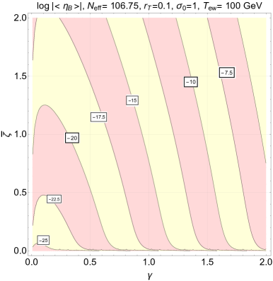
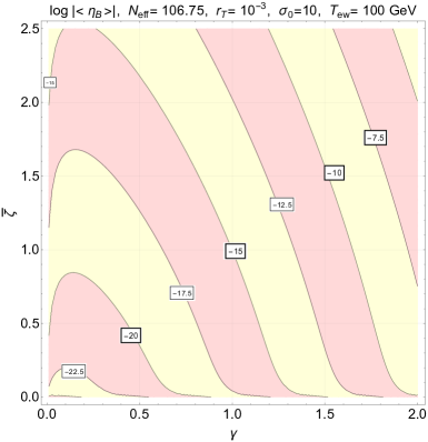
Figure 3: The contours of the common logarithm of the BAU are illustrated for a fiducial set of parameters assuming $T_{ew}=100\,\mathrm{GeV}$; note that $r_{T}=0.1$ (left plot) and $r_{T}=0.001$ (right plot).

While the contribution of the hypermagnetic gyrotropy determines the comoving baryon to entropy ratio $\eta_{B}=n_{B}/\varsigma$, the hyperelectric gyrotropy is washed out by the effect of the chiral conductivity. Denoting with $N_{eff}$ the effective number of relativistic degrees of freedom at the electroweak epoch and recalling the notations of Eqs. (3.12)–(3.13) the expression of the BAU [24, 25] is:

$$\eta_{B}(\vec{x},\tau)=\frac{n_{B}}{\varsigma}=\frac{3\alpha^{\prime}n_{f}}{8\pi\,H}\biggl{(}\frac{T}{\sigma}\biggl{)}\frac{{\mathcal{G}}^{(B)}(\vec{x},\tau)}{{\mathcal{H}}\,a^{4}\rho_{crit}},\qquad\qquad{\mathcal{G}}^{(B)}(\vec{x},\tau)=\vec{B}\cdot\vec{\nabla}\times\vec{B},$$ (6.1)

where $\varsigma=2\pi^{2}T^{3}N_{eff}/45$ is the entropy density of the plasma, $\alpha^{\prime}=g^{\prime 2}/(4\pi)$ (with $g^{\prime}\simeq 0.3$) is the $U(1)_{Y}$ coupling at the electroweak time and $n_{f}$ is the number of fermionic generations. In what follows $N_{eff}$ shall be fixed to its standard model value (i.e. $N_{eff}=106.75$). Equation (6.1) holds when the rate of the slowest reactions in the plasma (associated with the right-electrons) is larger than the dilution rate caused by the hypermagnetic field itself: at the phase transition the hypermagnetic gyrotropy is converted back into fermions since the ordinary magnetic fields does not couple to fermions. Since all quantities in Eq. (6.1) are comoving, $\langle\,\eta_{B}(\vec{x},\tau)\,\rangle$ for $\tau=\tau_{ew}$ is determined by the averaged gyrotropy:

$$\langle\,\eta_{B}(\vec{x},\tau_{ew})\,\rangle=\frac{3\,n_{f}\,\alpha^{\prime\,2}}{4\,\pi\sigma_{0}\,a_{ew}^{4}\,\rho_{crit}{\mathcal{H}}_{ew}}\int_{0}^{k_{\sigma}}\,P_{B}^{(G)}(k,\tau)\,dk,$$ (6.2)

where $\sigma_{0}$ accounts for the theoretical uncertainty associated with the determination of the chiral conductivity of the electroweak plasma according to $\sigma_{c}=\sigma_{0}T/\alpha^{\prime}$ [60, 61]. The upper limit of integration in Eq. (6.2) coincides with diffusivity momentum and it is useful to express $k_{\sigma}$ in units of ${\mathcal{H}}_{ew}=a_{ew}H_{ew}$ where $H_{ew}^{-1}={\mathcal{O}}(1)\,\mathrm{cm}$ is the Hubble radius at the electroweak time:

$$\frac{k_{\sigma}}{a_{ew}\,H_{ew}}=3.5\times 10^{8}\,\sqrt{\frac{\sigma_{0}}{\alpha^{\prime}\,N_{eff}}}\,\biggl{(}\frac{T_{ew}}{100\,\mathrm{GeV}}\biggr{)}^{-1/2}.$$ (6.3)

The typical diffusion scale exceeds the electroweak Hubble rate by approximately $8$ orders of magnitude and the corresponding range of wavelengths $\lambda_{\sigma}$ will roughly be smaller than ${\mathcal{O}}(10)$ nm (i.e. ${\mathcal{O}}(10^{-8})\mathrm{cm}$) at $\tau_{ew}$. By definition $x_{1}=k/(a_{1}H_{1})$ and $\tau_{ew}\simeq\tau\gg\tau_{1}$; thus the explicit expression of Eq. (4.54) becomes:

$$P_{B}^{(G)}(k,\tau)=a_{1}^{4}\,H_{1}^{4}\,D(\gamma+1/2)Q_{E}^{(G)}(\overline{\zeta},\gamma)\biggl{(}\frac{k}{a_{1}H_{1}}\biggr{)}^{4-2\gamma}\sin^{2}{k\tau}.$$ (6.4)

It is relevant to remark that Eq. (6.4) does not depend crucially on the approximation scheme but it is rather a direct consequence of the symmetries of the system (see in particular Eqs. (5.39)–(5.40) and discussion therein). Recalling now the average of the comoving gyrotropy computed in Eq. (3.13), the result of Eq. (6.4) leads to the wanted estimate of $\langle\,\eta_{B}(\vec{x},\tau_{ew})\,\rangle$:

$$\langle\,\eta_{B}(\vec{x},\tau_{ew})\,\rangle = \frac{2\,n_{f}\,\alpha^{\prime\,2}}{\sigma_{0}}\,\biggl{(}\frac{H_{1}}{M_{P}}\biggr{)}^{2}D(\gamma+1/2)Q_{E}^{(G)}(\overline{\zeta},\gamma)\biggl{(}\frac{a_{ew}\,H_{ew}}{a_{1}\,H_{1}}\biggr{)}^{4-2\gamma}{\mathcal{I}}(\gamma,k_{\sigma}),$$ (6.5)

$${\mathcal{I}}(\gamma,k_{\sigma}) = \int_{0}^{x_{\sigma}}\,\,x^{4-2\gamma}\,\,\sin^{2}{x}\,\,dx,\qquad x=\frac{k}{a_{ew}H_{ew}},\qquad x_{\sigma}=\frac{k_{\sigma}}{a_{ew}H_{ew}}.$$ (6.6)

Since the evolution between $\tau_{1}$ and $\tau_{ew}$ is dominated by radiation, in Eq. (6.5) we took into account that that $\rho_{crit}=3H_{ew}^{2}\overline{M}_{P}=3H_{1}^{2}\overline{M}_{P}(a_{1}/a_{ew})^{4}$ with $\overline{M}_{P}=M_{P}/\sqrt{8\pi}$. For the same reason we will also have that $(a_{ew}/a_{1})(H_{ew}/H_{1})=\sqrt{H_{ew}/H_{1}}$.

For the range of $k_{\sigma}$ entering Eq. (6.3) the integral ${\mathcal{I}}(\gamma,k_{\sigma})$ extends between $0$ and about $10^{8}$; as long as $\gamma\leq 2$, the integral of Eq. (6.6) is estimated as ${\mathcal{I}}(\gamma,k_{\sigma})=c_{\gamma}x_{\sigma}^{5-2\gamma}$ where $c_{\gamma}=1/[2(5-2\gamma)]$. This result is very accurate for $x_{\sigma}>10^{3}$ and $\gamma\leq 2$. For $x_{\sigma}=10^{3}$ and $\gamma=2$ the ratio between the exact and the approximate results is $0.9$ while it is practically $1$ as long as $x_{\sigma}>10^{3}$ for the whole range $0<\gamma\leq 2$. Taking into account this estimate and the other explicit figures mentioned above, the final expression of the BAU will be:

$$\langle\,\eta_{B}(\vec{x},\tau_{ew})\,\rangle = \frac{2\,n_{f}\,\alpha^{\prime\,2}}{\sigma_{0}}\,\biggl{(}\frac{H_{1}}{M_{P}}\biggr{)}^{\gamma}\biggl{(}\frac{H_{ew}}{M_{P}}\biggr{)}^{2-\gamma}\biggl{(}\frac{k_{\sigma}}{a_{ew}\,H_{ew}}\biggr{)}^{5-2\gamma}{\mathcal{J}}^{(G)}(\overline{\zeta},\gamma),$$ (6.7)

$${\mathcal{J}}^{(G)}(\overline{\zeta},\gamma) = \frac{2^{2\gamma-3}\Gamma^{2}(\gamma+1/2)}{\pi^{3}(5-2\gamma)}Q_{E}^{(G)}(\overline{\zeta},\gamma),$$ (6.8)

where, the function ${\mathcal{J}}^{(G)}(\overline{\zeta},\gamma)$ collects all the previously introduced numerical factors not related to the physical scales of the problem.

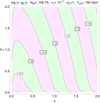
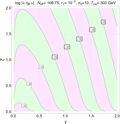
Figure 4: We illustrate the contours of the common logarithm of the BAU for larger values of $T_{ew}$ (i.e. $T_{ew}=150\,\mathrm{GeV}$ and $T_{ew}=300\,\mathrm{GeV}$) and for two extreme values of $\sigma_{0}$.

The quantities appearing in Eq. (6.7) can be easily related to the late-time cosmological parameters. In particular $H_{1}/M_{P}=\sqrt{\pi\,r_{T}\,{\mathcal{A}}_{{\mathcal{R}}}}/4$ where $r_{T}$ is the standard tensor to scalar ratio and ${\mathcal{A}}_{{\mathcal{R}}}=2.41\times 10^{-9}$ is the amplitude of the scalar power spectrum evaluated at the pivot scale $k_{p}=0.002\,\mathrm{Mpc}^{-1}$. The other two ratios of scales appearing in Eq. (6.7) follow directly from Eq. (6.3) and from the explicit value of $T_{ew}$ and $N_{eff}$, i.e. $H_{ew}/M_{P}=\sqrt{4\pi^{3}N_{eff}/45}(T_{ew}/M_{P})^{2}$. The common logarithm of the BAU for a reference temperature of $100$ GeV is illustrated in Fig. 3 for different values of $r_{T}$. While the physical range of values of $r_{T}$ is below $10^{-2}$ [62, 63], a drastic decrease in $r_{T}$ (e.g. $r_{T}={\mathcal{O}}(10^{-4})$) has a mild impact on the numerical value of the BAU since $\eta_{B}\propto r_{T}^{\gamma/2}$. The interesting region of the parameter space is the one where $\eta_{B}$ is larger than $10^{-10}$: indeed we have to foresee the BAU might be diluted depending on the specific dynamics of the phase transition. In Fig. 4 a different range of temperatures is illustrated but the features of the contours are fully compatible with the ones of Fig. 3. It is finally useful to remark that $\sigma_{0}$ parametrizes, in practice, the indetermination in the estimate of $\sigma_{c}$ and this is why we shall assume that $1\leq\sigma_{0}\leq 10$. Both in Figs. 3 and 4 different values of $\sigma_{0}$ have been selected just for the sake of illustration. The baryon asymmetry produced on this way has a number of further consequences which have been partially investigated in the past [64, 65, 66]. These discussions are beyond the scopes of the present discussion whose main purpose is to chart the parameter space of a potentially interesting scenario.

6.3 Requirements from magnetogenesis

The considerations associated with the BAU involved typical $k$-modes in the range $a_{ew}\,H_{ew}\leq k<k_{\sigma}$. While the modes inside the Hubble radius at the electroweak time reentered right after inflation, for the effects related to magnetogenesis the relevant comoving scales are of the order of the Mpc at the epoch of the gravitational collapse of the protogalaxy, the corresponding wavelengths reentered the effective horizon just prior to matter-radiation equality. If$\tau_{k}=1/k$ denotes the reentry time of a generic wavelength, the ratio between $\tau_{k}$ and the time of matter-radiation equality $\tau_{eq}$ is:

$$\frac{\tau_{k}}{\tau_{eq}}=1.06\times 10^{-6}\biggl{(}\frac{h_{0}^{2}\Omega_{M0}}{0.1386}\biggr{)}\biggl{(}\frac{h_{0}^{2}\Omega_{R0}}{4.15\times 10^{-5}}\biggr{)}^{-1/2}\,\biggl{(}\frac{k}{\mathrm{Mpc}^{-1}}\biggr{)}^{-1},$$ (6.9)

since $(\tau_{k}/\tau_{eq})=\sqrt{2}(H_{0}/k)\Omega_{M0}/\Omega_{R0}$. Even if the reentry of the the Mpc scales occurred much later than the electroweak time, Eq. (6.9) shows that, within the concordance paradigm, the wavenumbers $k={\mathcal{O}}(\mathrm{Mpc}^{-1})$ still reentered prior to matter radiation equality. We shall assume that the gauge coupling freezes at $\tau_{k}$ even if this is not strictly necessary. In fact for $\tau>\tau_{k}$ the conductivity dominates and the duality symmetry is further broken because of the presence of Ohmic currents,

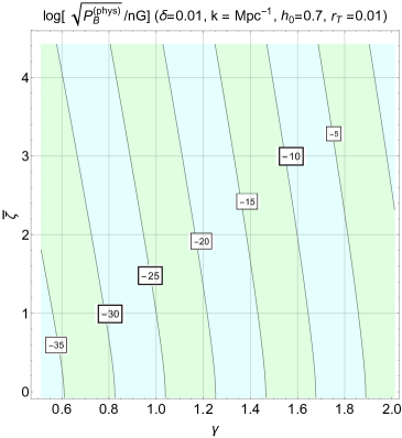
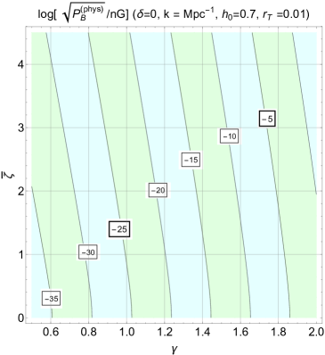
Figure 5: The parameter space is illustrated in the $(\gamma,\,\overline{\zeta})$ plane. The numbers appearing on the various contours correspond to the common logarithm of $\sqrt{P_{B}^{(phys)}}$ expressed in nG units.

so that the evolution of the magnetic and of the electric mode functions is very different: while the electric fields are suppressed by the finite value of the conductivity, the magnetic fields are not dissipated at least for typical scales smaller than the magnetic diffusivity scale. In practice the mode functions for $\tau\geq\tau_{k}$ will be suppressed with respect to their values at $\tau_{k}$ as:

$$f_{k}(\tau)=f_{k}(\tau_{k})e^{-k^{2}/k_{d}^{2}},\qquad g_{k}(\tau)=(k/\sigma_{em})g_{k}(\tau_{k})e^{-k^{2}/k_{d}^{2}},\qquad k_{d}^{-2}=\int_{\tau_{k}}^{\tau}\,\,d\,z/\sigma_{em}(z),$$ (6.10)

where $\sigma_{em}$ is the standard conductivity of the plasma (to be distinguished from its chiral counterpart $\sigma_{c}$ discussed above) and $k_{d}$ denotes the magnetic diffusivity momentum. The ratio $(k/k_{d})^{2}$ appearing in Eq. (6.10) is actually extremely small in the phenomenologically interesting situation; $\tau=\tau_{\mathrm{eq}}$ the ratio $(k/k_{d})^{2}$ turns out to be:

$$\biggl{(}\frac{k}{k_{d}}\biggr{)}^{2}=\frac{4.75\times 10^{-26}}{\sqrt{2\,h_{0}^{2}\Omega_{M0}(z_{\mathrm{eq}}+1)}}\,\biggl{(}\frac{k}{\mathrm{Mpc}^{-1}}\biggr{)}^{2},$$ (6.11)

where $\Omega_{M0}$ is the present critical fraction in dusty matter and $z_{\mathrm{eq}}+1=a_{0}/a_{\mathrm{eq}}\simeq{\mathcal{O}}(3200)$ is the redshift of matter-radiation equality. The magnetic spectrum for $k<k_{d}$ is practically not affected by the conductivity while the electric power spectrum is suppressed by $k^{2}/\sigma_{em}^{2}\ll 1$.

If a given quantity is not affected by the expansion of the background the comoving and physical fields could be used interchangeably. For instance in the case of the BAU $n_{B}$ (i.e. the baryon concentration) and $\varsigma$ (the entropy density) redshift in the same way so that $\eta_{B}$ could be computed directly in terms of the comoving fields. What matters for the magnetogenesis requirements are the instead physical power spectra prior to gravitational collapse since we now have to compare the values of the power spectra with a set of bounds valid at a given time. Recalling Eq. (2.4) we have that the physical power spectrum is:

$$P_{B}^{(phys)}(k,\tau)=\frac{P_{B}(k,\tau)}{a^{4}\lambda}\,\cos^{2}{\theta_{W}},\qquad\Rightarrow\quad P_{B}^{(phys)}(k,\tau_{*})=\frac{P_{B}(k,\tau_{k})}{a_{k}^{4}\lambda_{k}}\biggl{(}\frac{a_{k}}{a_{*}}\biggr{)}^{4}\,\cos^{2}{\theta_{W}}.$$ (6.12)

The first expression of Eq. (6.12) is just the definition of the physical power spectrum obtained directly from Eq. (2.4) by evaluating, after symmetry breaking, the two-point function of Eq. (3.6) in terms of the physical fields. The second expression appearing in Eq. (6.12) is instead the physical power spectrum computed at a reference time $\tau_{*}>\tau_{k}$ under the further assumption that the gauge coupling is effectively frozen for $\tau>\tau_{k}$.

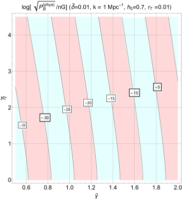
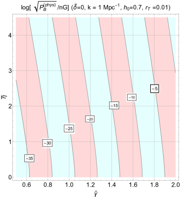
Figure 6: The parameter space is illustrated in the $(\widetilde{\gamma},\,\overline{\eta})$ plane. As in Fig. 3 the numbers appearing on the various contours correspond to the common logarithm of $\sqrt{P_{B}^{(phys)}}$ expressed in nG units.

Even though the parameter space is easily charted by varying the relevant physical parameters, it is useful, in a preliminary perspective, to discuss the orders of magnitude of the problem by evaluating the physical counterpart of the comoving spectrum given in Eq. (4.52). Inserting then Eq. (4.52) into Eq. (6.12) we obtain:

$$P_{B}^{(phys)}(k,\tau_{*}) = \frac{H_{1}^{4}}{\lambda_{1}}\biggl{(}\frac{a_{1}}{a_{k}}\biggr{)}^{4}\,\biggl{(}\frac{a_{k}}{a_{*}}\biggr{)}^{4}\biggl{(}\frac{k}{a_{1}H_{1}}\biggr{)}^{4-2\gamma}{\mathcal{J}}(\overline{\zeta},\gamma)\cos^{2}{\theta_{W}}\,\,\sin^{2}{k\tau_{k}},$$

$${\mathcal{J}}(\overline{\zeta},\gamma) = Q_{E}(\overline{\zeta},\gamma)D(\gamma+1/2),$$ (6.13)

where we considered, for the sake of simplicity, the situation where $\delta\ll\gamma$ so that the evolution of $\lambda$ could be effectively neglected for $\tau\geq-\tau_{1}$. The order of magnitude of the physical power spectrum does not have to coincide with the observed values the magnetic fields of the galaxies (or of the clusters). The way large-scale magnetic fields originate is a rather broad subject that will not be discussed here in detail; various more specific discussions exist (see e. g. [67, 68, 69]). In a conservative perspective the magnetogenesis requirements roughly demand that the magnetic fields at the time of the gravitational collapse of the protogalaxy should be approximately larger than a (minimal) power spectrum which can be estimated between ${\mathcal{O}}(10^{-32})\,\mathrm{nG}^{2}$ and ${\mathcal{O}}(10^{-22})\,\mathrm{nG}^{2}$:

$$\log{\biggl{(}\frac{\sqrt{P^{(phys)}_{B}(k,\tau_{*})}}{\mathrm{nG}}\biggr{)}}\geq-\omega,\qquad 11<\omega<16.$$ (6.14)

The least demanding requirement of Eq. (6.14) (i.e. $\sqrt{P^{(phys)}_{B}(k,\tau_{*})}\geq 10^{-16}\,\mathrm{nG}$) follows by assuming that, after compressional amplification, every rotation of the galaxy increases the initial magnetic field of one $e$-fold. According to some this requirement is not completely realistic since it takes more than one $e$-fold to increase the value of the magnetic field by one order of magnitude and this is the rationale for the most demanding condition of Eq. (6.14), i.e. $\sqrt{P^{(phys)}_{B}}\geq 10^{-11}\,\mathrm{nG}$.

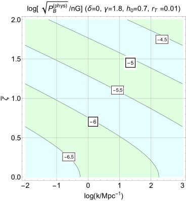
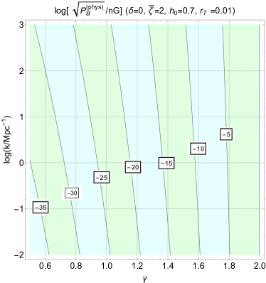
Figure 7: The parameter space is illustrated in the case of increasing gauge coupling and for different comoving scales. As in the previous plots the numbers appearing on the various contours correspond to the common logarithm of $\sqrt{P_{B}^{(phys)}}$ expressed in nG units.

It is now useful to estimate the overall amplitude of Eq. (6.13) and to compare the obtained result with the conditions of Eq. (6.14). For this purpose let us neglect, for a moment, the scale dependence of Eq. (6.13) and focus on the overall amplitude; in this case we will have that

$$\sqrt{P^{(phys)}_{B}(k,\tau_{*})}=\frac{H_{1}^{2}}{\lambda_{1}}\biggl{(}\frac{a_{1}}{a_{*}}\biggr{)}^{2}\cos^{2}{\theta_{W}}\simeq\frac{e_{1}\sqrt{\pi}}{32}\,r_{T}\,{\mathcal{A}}_{{\mathcal{R}}}\,M_{P}^{2}\,\biggl{(}\frac{a_{1}}{a_{*}}\biggr{)}^{2}\cos^{2}{\theta_{W}},$$ (6.15)

where, as before, we traded $(H_{1}/M_{P})^{2}$ for $\pi r_{T}{\mathcal{A}}_{{\mathcal{R}}}/16$ and recalled the definition of the gauge coupling at $\tau_{1}$ (i.e. $e_{1}=\sqrt{4\pi/\lambda_{1}}$). Equation (6.15) should now be expressed in units of nG and, for this purpose, we recall that $M_{P}^{2}=2.15\times 10^{-66}\,\,\mathrm{nG}$. The final result for Eq. (6.15) can therefore be written as:

$$\sqrt{P^{(phys)}_{B}(k,\tau_{0})}=4.89\times 10^{-4}\biggl{(}\frac{r_{T}}{0.01}\biggr{)}^{1/2}\,\biggl{(}\frac{{\mathcal{A}}_{{\mathcal{R}}}}{2.41\times 10^{-9}}\biggr{)}^{1/2}\,\biggl{(}\frac{h_{0}^{2}\Omega_{R0}}{4.15\times 10^{-5}}\biggr{)}^{1/2}\,\,\,\mathrm{nG}.$$ (6.16)

Even if the figures of Eq. (6.14) seem even too large in comparison with Eq. (6.16) a substantial reduction comes from the scale dependence that can be estimated by following exactly the same strategy outlined before. The relevant result is:

$$\frac{k}{a_{1}\,H_{1}}=10^{-23.05}\,\,\biggl{(}\frac{k}{\mathrm{Mpc}^{-1}}\biggr{)}\,\biggl{(}\frac{r_{T}}{0.01}\biggr{)}^{-1/4}\,\,\biggl{(}\frac{h_{0}^{2}\Omega_{R0}}{4.15\times 10^{-5}}\biggr{)}^{-1/4}\,\,\biggl{(}\frac{{\mathcal{A}}_{{\mathcal{R}}}}{2.41\times 10^{-9}}\biggr{)}^{-1/4}.$$ (6.17)

Last but not least the physical power spectrum will be further affected by ${\mathcal{J}}(\overline{\zeta},\gamma)$ which cannot be evaluated in its asymptotic limit since both $\overline{\zeta}$ and $\gamma$ are both quantities ${\mathcal{O}}(1)$; indeed the most interesting region of the parameter space (i.e. where the constraints of Figs. 1 and 2 are satisfied) occurs for relatively modest values of the anomalous interactions. We shall therefore analyze the physical power spectra in numerical terms: the values of the common logarithm of the physical power spectra will be discussed for the different values of the parameters. In Fig. 5 and in all the forthcoming figures the labels denote $\sqrt{P_{B}^{(phys)}}$ in units on nG. In Fig. 5 the physical power spectrum is illustrated in the $(\gamma,\overline{\zeta})$ plane: in both plots the gauge coupling increases during inflation and then flattens out by always remains smaller than $1$; however in the plot at the left $\delta=0.01$ while in the plot at the right $\delta\to 0$. In the subsequent plots these two conceptually different physical situations will be often distinguished with the purpose of stressing that that the numerical differences are minimal.

The critical density constraint discussed in Fig. 1 would imply that $\overline{\zeta}={\mathcal{O}}(\gamma)$ and also, somehow, that $\zeta\leq 2$. By looking at the intercept on the $\gamma$ axis we see that the phenomenologically reasonable values of $\gamma$ correspond to spectra that are blue or, at most, quasi-flat but always slightly increasing with $k$. The effect of non-vanishing $\overline{\zeta}$ can be appreciated by comparing a five value of $\gamma$ for different values of $\overline{\zeta}$: the increase of $\overline{\zeta}$ from $0$ to $2$ or even $3$ is not crucial in order to satisfy the magnetogenesis constraints and it can be traded for an increase in $\gamma$.

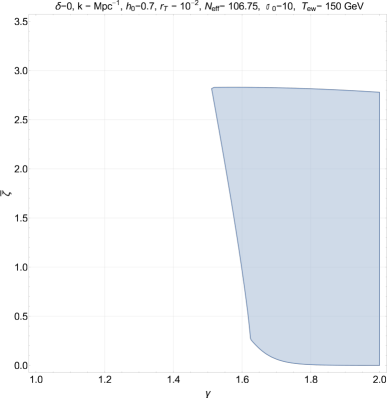
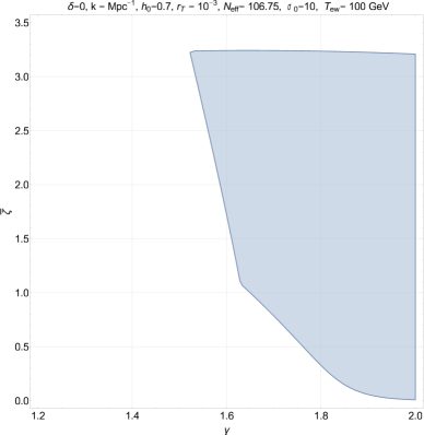
Figure 8: The shaded area illustrates the region of the parameter space where the baryogenesis and the magnetogenesis constraints are simultaneously satisfied.

In Fig. 6 we instead illustrated the $(\widetilde{\gamma},\overline{\eta})$ plane: in this case the physical features seem roughly the same but there is actually an important difference. Both in Figs. 5 and 6 the gauge coupling is ${\mathcal{O}}(1)$ for $\tau=-\tau_{1}$. However in the case of Fig. 6 the gauge coupling decreases so that at the initial time of the evolution had to be much larger, possibly in the strongly coupled regime of the model. To be compatible with the strong coupling limit we should therefore require that $\sqrt{\lambda_{1}}$ is much larger than $1$. But since $\lambda_{1}$ enters the definition of the physical spectrum the results of Fig. 6 has to be reduced by a factor that must reduce the initially larger value of the gauge coupling . Typically for an inflationary phase characterized by $N={\mathcal{O}}(60)$ $e$-folds the results of Fig. 6 are suppressed by a factor $e^{-2\widetilde{\gamma}N}$. This reduction is not present in the case of increasing coupling where, depending on the specific scenario, $e_{1}=\sqrt{4\pi/\lambda_{1}}={\mathcal{O}}(0.01)$.

Both in Figs. 5 and 6 the typical comoving scale of the spectrum has been fixed to the Mpc value. The variation of the comoving scale is considered in Fig. 7 and in the case of increasing gauge coupling. In Fig. 7 we illustrate two different slices of the parameter space namely the $(k,\,\overline{\zeta})$ and the $(k,\,\gamma)$ planes. In both plots we assumed, for the sake of simplicity, $\delta\to 0$. As expected, for fixed $\overline{\zeta}$ the values of the physical spectra are progressively reduced as $\gamma$ decreases. However $\gamma={\mathcal{O}}(1.6)$ are still viable. Conversely, for fines $\gamma$, the value of the power spectra increase with $\overline{\zeta}$ which is however constrained from above by the critical density limits discussed in Fig. 1.

We finally plot in Fig. 8 the region of the parameter space of the scenario where the baryogenesis and the magnetogenesis constraints are simultaneously satisfied. As we can see by comparing the two classes of requirements, different choices of the parameters lead to similar regions in the $(\gamma,\,\overline{\zeta})$ plane. The shaded areas in Fig. 8 correspond to the situation where the values of the BAU are larger than $10^{-10}$ while the magnetogenesis constraints are satisfied. We stress that larger values of the BAU are phenomenologically safer since, after the electroweak epoch, different physical processes can release entropy and further reduce the generated BAU.

7 Concluding remarks

The production of hypermagnetic gyrotropy has been investigated when the gauge coupling continuously interpolates between a quasi-de Sitter stage of expansion and the radiation phase without entering a strongly coupled regime. Since during the inflationary epoch the strength of anomalous interactions is constrained also the hyermagnetic gyrotropy is indirectly bounded.

The logic followed in similar situations has been purposely reversed: instead of fixing the couplings and then deducing the potential phenomenological implications we treated the strength of the pseudoscalar interactions as a free parameter that must be simultaneously compatible with the critical energy density constraints and with the perturbative evolution of the gauge coupling. Even though the primary focus has been the case where the gauge coupling increases and then flattens out in the perturbative region, we also found relevant to address the dual evolution where at the beginning of inflation the gauge coupling is potentially strong. From the mutual interplay of these dual scenarios it turns out that the would be duality symmetry still exchanges hypermagnetic spectra and hyperelectric spectra even if the reciprocal transformation is not realized. This collateral observation ultimately determines the late-time form of the gauge spectra.

The gauge modes reentering at different times during the radiation-dominated phase impact both the symmetric and the broken phases of the electroweak theory. In the plane defined by the strength of the anomalous interaction and by the rate of evolution of the gauge coupling the actual weight of the pseudoscalar terms suffices to produce an average hypermagnetic gyrotropy whose decay determines the BAU below the electroweak temperature. While the modes contributing to the hypermagnetic gyrotropy are all inside the effective horizon before the electroweak time, the modes reentering just prior to matter-radiation equality also generate large-scale magnetic fields in the nG range. According to perspective developed here the strength of the pseudoscalar interactions required by the magnetogenesis considerations is compatible with the all the other constraints derived both during the quasi-de Sitter stage and at the electroweak epoch. While the present proposal is admittedly less conventional than the standard realizations of baryogenesis and leptogenesis we showed here that it can be implemented in a rather plausible framework which is generally allowed by the relevant phenomenological constraints.

Appendix A Left and Right mode functions and their normalizations

To avoid lengthy digressions, in the two sections of this appendix a general discussion of the circularly polarized mode functions shall be presented. These considerations will be probably useful for the interested readers but are technically essential for the derivation of all the major results discussed in the bulk of the paper. In the case of increasing gauge coupling the evolution of $\sqrt{\lambda}$ follows Eqs. (4.1)–(4.2) and for $\tau\leq-\tau_{1}$ the explicit form of Eqs. (2.18)–(2.19) is:

$$f_{k,\,L}^{\,\prime\prime}+\biggl{[}k^{2}-\frac{\gamma(\gamma-1)}{\tau^{2}}-\frac{\lambda_{0}\,k\,\gamma}{\tau}\biggr{]}f_{k,\,L}=0,\qquad f_{k,\,R}^{\,\prime\prime}+\biggl{[}k^{2}-\frac{\gamma(\gamma-1)}{\tau^{2}}+\frac{\lambda_{0}\,k\,\gamma}{\tau}\biggr{]}f_{k,\,R}=0.$$ (A.1)

Once the hypermagnetic mode functions have been determined from the normalized solutions of Eq. (A.1), the hyperelectric mode functions will be deduced from the following pair of relations ultimately coming from the definition of the canonical field operators:

$$g_{k,\,L}=f_{k,\,L}^{\,\prime}-\frac{\gamma}{\tau}f_{k,\,L},\qquad g_{k,\,R}=f_{k,\,R}^{\,\prime}-\frac{\gamma}{\tau}f_{k,\,R}.$$ (A.2)

By now introducing the rescaled quantities defined in Eq. (4.6) (i.e. $z=2\,i\,k\,\tau$ , $\zeta=i\,\lambda_{0}\,\gamma$ and $\mu=|\gamma-1/2|$) the explicit form of Eq. (4.5) is recovered and it coincides with the standardized form of the Whittaker’s equation. We follow, in this respect, the notations of Ref. [47] but very similar notations for the Whittaker’s equation can be found in other treatments and they all ultimately coincide with the classic discussion of confluent hypergeometric functions of Whittaker and Watson [70]. In the case of decreasing gauge coupling $\sqrt{\lambda}$ follows instead Eqs. (5.1)–(5.2) and for $\tau\leq-\tau_{1}$ Eqs. (2.18)–(2.19) become:

$$f_{k,\,L}^{\,\prime\prime}+\biggl{[}k^{2}-\frac{\widetilde{\gamma}(\widetilde{\gamma}+1)}{\tau^{2}}-\frac{2\,\lambda_{0}\,k\,\widetilde{\gamma}}{\tau}\biggr{]}f_{k,\,L}=0,\qquad f_{k,\,R}^{\,\prime\prime}+\biggl{[}k^{2}-\frac{\widetilde{\gamma}(\widetilde{\gamma}+1)}{\tau^{2}}+\frac{2\,\lambda_{0}\,k\,\widetilde{\gamma}}{\tau}\biggr{]}f_{k,\,R}=0.$$ (A.3)

We recall here the convention adopted in the bulk of the paper: all the quantities with tilde refer to the case of decreasing gauge coupling since this notation turns out to be quite useful when discussing the duality properties of the gauge power spectra. From Eq. (A.3) the hyperelectric mode functions are instead:

$$g_{k,\,L}=f_{k,\,L}^{\,\prime}+\frac{\widetilde{\gamma}}{\tau}f_{k,\,L},\qquad g_{k,\,R}=f_{k,\,R}^{\,\prime}+\frac{\widetilde{\gamma}}{\tau}f_{k,\,R}.$$ (A.4)

From Eqs. (A.3)–(A.4) the canonical expressions of the Whittaker’s equations (5.5) is recovered by using the variables of Eq. (5.6). Since the circularly polarized mode functions are related to the standardized form of the Whittaker’s equation, the most relevant properties will now be listed [47]. If the Whittaker’s equation is written in its canonical form as:

$$\frac{d^{2}h}{dz^{2}}+\biggl{[}-\frac{1}{4}+\frac{\alpha}{z}-\frac{\sigma^{2}-1/4}{z^{2}}\biggr{]}h=0,$$ (A.5)

the two linearly independent solutions of Eq. (A.5) are $W_{\alpha,\sigma}(z)$ and $W_{-\alpha,\sigma}(-z)$. For $|z|\gg 1$ the asymptotic limit is $W_{\alpha,\sigma}(z)\to e^{-z/2}z^{\alpha}$. According to Eqs. (4.6) and (5.6) the variable $z$ is actually defined as $z=2i\,k\,\tau$ so that the limit of $W_{\zeta,\mu}(z)$ for $|z|\gg 1$ is actually a distorted plane wave. In the opposite limit $z\ll 1$

$$W_{\alpha,\sigma}(z)=z^{1/2-\sigma}\biggl{[}\frac{\Gamma(2\sigma)}{\Gamma\left(1/2+\sigma-\alpha\right)}+\frac{\alpha\,z\Gamma(2\sigma-1)}{\Gamma\left(1/2+\sigma-\alpha\right)}+{\mathcal{O}}\left(z^{5/2}\right)\biggr{]}.$$ (A.6)

The Hankel limit of the Whittaker’s functions (i.e. $\alpha\to 0$) allows for a direct connection between the, the modified Bessel functions and the Hankel functions [47]:

$$\lim_{\alpha\to 0}W_{\alpha,\sigma}(z)=\sqrt{\frac{z}{\pi}}K_{\sigma}(z/2),$$ (A.7)

where $K_{\sigma}(z/2)$ are the modified Bessel functions whose analytic continuation is directly related to the Hankel functions of first and second kind:

$$K_{\sigma}(z/2) = \frac{i\,\pi}{2}e^{i\,\pi\,\sigma/2}\,H_{\sigma}^{(1)}(ze^{i\,\pi/2}/2),\qquad-\pi<\mathrm{arg}z\leq\pi/2,$$ (A.8)

$$K_{\sigma}(z/2) = -\frac{i\,\pi}{2}e^{-i\,\pi\,\sigma/2}\,H_{\sigma}^{(2)}(ze^{-i\,\pi/2}/2),\qquad-\pi/2<\mathrm{arg}z\leq\pi.$$ (A.9)

Equations (A.7) and (A.8)–(A.9) are essential to recover the correct Hankel limit of various expressions (see e.g. Eqs. (4.10)). Furthermore the explicit expressions for the matrix elements reported in Eq. (4.43) can be swiftly derived by recalling since $H_{\sigma}^{(1)}(w)=J_{\sigma}(w)+iY_{\sigma}(w)=H_{\sigma}^{(2)\ast}(w)$. When doing the various analytic continuations it is useful to bear in mind that during the quasi-de Sitter stage $\tau$ is negative while it is positive in the post-inflationary stage of expansion [see e.g. Eq. (4.4) and discussion thereafter]. When the gauge coupling increases during a quasi-de Sitter stage of expansion the approximate expressions of the mode functions given in Eqs. (4.7)–(4.11) and (4.12) can be derived in the limit $-\,k\tau\ll 1$

$$f_{k,\,L}(\tau) = \frac{e^{-\pi\overline{\zeta}/2}\,\,e^{i\pi\mu/2}}{\sqrt{2k}}\,\frac{\Gamma(2\mu)\,(-\,2k\tau)^{1/2-\mu}}{\Gamma(1/2+\mu-i\,\overline{\zeta})},$$

$$f_{k,\,R}(\tau) = \frac{e^{\pi\overline{\zeta}/2}}{\,}\,e^{i\pi(\mu-1)/2}{\sqrt{2k}}\,\frac{\Gamma(2\mu)\,(-\,2k\tau)^{1/2-\mu}}{\Gamma(1/2+\mu+i\,\overline{\zeta})},$$ (A.10)

$$g_{k,\,L}(\tau) = \sqrt{2k}\,e^{-\pi\overline{\zeta}/2}\,\,e^{i\pi(\gamma-1/2)/2}\,\frac{\Gamma(2\gamma)\,(-\,2k\tau)^{-\gamma}}{\Gamma(\gamma-i\overline{\zeta})},$$

$$g_{k,\,R}(\tau) = \sqrt{2k}\,e^{\pi\overline{\zeta}/2}\,\,e^{i\pi(\gamma+1/2)/2}\,\frac{\Gamma(2\gamma)\,(-\,2k\tau)^{-\gamma}}{\Gamma(\gamma+i\overline{\zeta})};$$ (A.11)

note that, only for practical reasons, in Eq. (A.10) we used directly the quantity $\mu=|\gamma-1/2|$. The obtained expressions can be further simplified thanks to the standard duplication formulas for the Gamma function [i.e. $\Gamma(2\sigma)=2^{2\sigma-1/2}\Gamma(\sigma)\Gamma(\sigma+1/2)/\sqrt{2\pi}$]. In the limit $\overline{\zeta}\gg 1$ Eqs. (A.10)–(A.11) can also be evaluated with the standard asymptotic expressions valid in the case of the standard Gamma functions. When the gauge coupling decreases during the quasi-de Sitter stage the limits of the hypermagnetic and hyperelectric mode functions for $-k\tau\ll 1$ are instead:

$$f_{k,\,L}(\tau) = \frac{e^{\pi\overline{\eta}/2}\,\,e^{i\,\pi(\,\widetilde{\gamma}+1/2)/2}}{\sqrt{2k}}\,(-\,2k\tau)^{-\widetilde{\gamma}}\,\frac{\Gamma(2\widetilde{\gamma}+1)}{\Gamma(1+\widetilde{\gamma}+i\,\overline{\eta})},$$ (A.12)

$$f_{k,\,R}(\tau) = \frac{e^{-\pi\overline{\eta}/2}\,\,e^{i\,\pi(\,\widetilde{\gamma}-1/2)/2}}{\sqrt{2k}}\,(-\,2k\tau)^{-\widetilde{\gamma}}\,\frac{\Gamma(2\widetilde{\gamma}+1)}{\Gamma(1+\widetilde{\gamma}-i\,\overline{\eta})},$$ (A.13)

$$g_{k,\,L}(\tau) = \frac{\sqrt{2k}\,e^{\pi\overline{\eta}/2}\,e^{i\,\pi(\,\widetilde{\gamma}+1/2)/2}}{\Gamma(1+\widetilde{\gamma}+i\overline{\eta})}\,(\,2k\tau)^{-\widetilde{\gamma}}\,\biggl{[}\overline{\eta}\Gamma(2\widetilde{\gamma})-(\widetilde{\gamma}-1)(2\overline{\eta}^{2}+\widetilde{\gamma})\Gamma(2\widetilde{\gamma}-2)(-\,k\tau)+{\mathcal{O}}(k^{2}\tau^{2})\biggr{]}$$ (A.14)

$$+ (-2k\tau)^{\widetilde{\gamma}}\biggl{[}\frac{\sqrt{2k}\,e^{\pi\overline{\eta}/2}\,e^{-i\,\pi(\,\widetilde{\gamma}+1/2)/2}\Gamma(-2\widetilde{\gamma})}{\Gamma(i\overline{\eta}-\widetilde{\gamma})}+{\mathcal{O}}(k\tau)\biggr{]},$$

$$g_{k,\,R}(\tau) = \frac{\sqrt{2k}\,e^{-\pi\overline{\eta}/2}\,e^{i\,\pi(\,\widetilde{\gamma}-1/2)/2}}{\Gamma(1+\widetilde{\gamma}-i\overline{\eta})}\,(-2k\tau)^{-\widetilde{\gamma}}\,\biggl{[}-\overline{\eta}\Gamma(2\widetilde{\gamma})+(\widetilde{\gamma}-1)(2\overline{\eta}^{2}+\widetilde{\gamma})\Gamma(2\widetilde{\gamma}-2)(-k\tau)+{\mathcal{O}}(k^{2}\tau^{2})\biggr{]}$$ (A.15)

$$- (-\,2k\tau)^{\widetilde{\gamma}}\biggl{[}\frac{\sqrt{2k}\,e^{-\pi\overline{\eta}/2}e^{-i\,\pi(\,\widetilde{\gamma}-1/2)/2}\,\Gamma(-2\widetilde{\gamma})}{\Gamma(-i\overline{\eta}-\widetilde{\gamma})}+{\mathcal{O}}(k\tau)\biggr{]}.$$

Note that in the asymptotic expression of Eqs. (A.14)–(A.15) the effective expansion parameter is in fact represented by $(-k\tau)\,\overline{\eta}<1$. As in the case of Eqs. (A.10) and (A.11) the expansions are valid in the long wavelength limit also when $\overline{\eta}\gg 1$ as long as $|k\tau|<1/\overline{\eta}$.

Appendix B Late-time forms of the mode functions

Both when the gauge coupling increases and decreases the late-time form of the mode functions could be expressed as the superposition of the two linearly independent solutions of the homogeneous Whittaker’s equation:

$$f_{k,\,X}=A_{-}\,\overline{F}^{(2)}_{k,\,X}+A_{+}\,\overline{F}^{(1)}_{k,\,X},\qquad g_{k,\,L}=A_{-}\,\overline{G}^{(2)}_{k,\,X}+A_{+}\,\overline{G}^{(1)}_{k,\,X},$$ (B.1)

where $X=L,\,R$ and ($F_{k,\,X}^{(1)}$, $F_{k,\,X}^{(2)}$) and ($G_{k,\,X}^{(1)}$, $G_{k,\,X}^{(2)}$) denote the two linearly independent solutions for $\tau\geq-\tau_{1}$. In the case of increasing gauge coupling the normalized form of the linearly independent solutions follows from Eqs. (4.29) and (4.30). For the $L$-polarization the results are

$$F_{k\,L}^{(1)}(\tau)=D^{(1)}_{L}(k,\overline{\xi})\,W_{\xi,\,\nu}(w),\qquad F_{k\,L}^{(2)}(\tau)=D^{(2)}_{L}(k,\overline{\xi})\,W_{-\xi,\,\nu}(-w),$$ (B.2)

$$G_{k,\,L}^{(1)}(\tau)=2\,i\,k\,D^{(1)}_{L}(k,\overline{\xi})\biggl{[}\frac{w-2\xi+2\delta}{2w}W_{\xi,\,\nu}(w)-\frac{W_{1+\xi,\,\nu}(w)}{w}\biggr{]},$$ (B.3)

$$G_{k,\,L}^{(2)}(\tau)=2\,i\,k\,D^{(2)}_{L}(k,\overline{\xi})\biggl{[}\frac{-w+2\xi+2\delta}{2w}W_{-\xi,\,\nu}(-w)-\frac{W_{1-\xi,\,\nu}(-w)}{w}\biggr{]},$$ (B.4)

In the case of the $R$-polarization the solutions are instead

$$F_{k\,R}^{(1)}(\tau)=D^{(1)}_{R}(k,\overline{\xi})\,W_{-\xi,\,\nu}(w),\qquad F_{k\,R}^{(2)}(\tau)=D^{(2)}_{R}(k,\overline{\xi})\,W_{\xi,\,\nu}(-w),$$ (B.5)

$$G_{k,\,R}^{(1)}(\tau)=2\,i\,k\,D^{(1)}_{R}(k,\overline{\xi})\biggl{[}\frac{(w+2\xi+2\delta)}{2w}W_{-\xi,\,\nu}(w)-\frac{W_{1-\xi,\,\nu}(w)}{w}\biggr{]},$$ (B.6)

$$G_{k,\,R}^{(2)}(\tau)=2\,i\,k\,D^{(2)}_{R}(k,\overline{\xi})\biggl{[}\frac{(-w-2\xi+2\delta)}{2w}W_{\xi,\,\nu}(-w)-\frac{W_{1+\xi,\,\nu}(-w)}{w}\biggr{]}.$$ (B.7)

The normalization appearing in Eqs. (B.2)– (B.4) and (B.5)–(B.7) are:

$$D_{L}^{(1)}(k,\overline{\xi})=\frac{e^{i\pi/4+\pi\overline{\xi}/2}}{\sqrt{2k}},\qquad D_{L}^{(2)}(k,\overline{\xi})=\frac{e^{-i\pi/4+\pi\overline{\xi}/2}}{\sqrt{2k}},$$

$$D_{R}^{(1)}(k,\overline{\xi})=\frac{e^{-i\pi/4-\pi\overline{\xi}/2}}{\sqrt{2k}},\qquad D_{R}^{(2)}(k,\overline{\xi})=\frac{e^{i\pi/4-\pi\overline{\xi}/2}}{\sqrt{2k}}.$$ (B.8)

The same procedure can be repeated in the case of decreasing gauge coupling and the result go as follows:

$$\widetilde{F}_{k\,L}^{(1)}(\tau)=\widetilde{D}^{(1)}_{L}(k,\overline{\theta})\,W_{-\theta,\,\widetilde{\nu}}(w),\qquad\widetilde{F}_{k\,L}^{(2)}(\tau)=\widetilde{D}^{(2)}_{L}(k,\overline{\theta})\,W_{\theta,\,\widetilde{\nu}}(-w),$$ (B.9)

$$\widetilde{G}_{k,\,L}^{(1)}(\tau)=2\,i\,k\,\widetilde{D}^{(1)}_{L}(k,\overline{\theta})\biggl{[}\frac{w+2\theta-2\widetilde{\delta}}{2w}W_{-\theta,\,\widetilde{\nu}}(w)-\frac{W_{1-\theta,\,\widetilde{\nu}}(w)}{w}\biggr{]},$$ (B.10)

$$\widetilde{G}_{k,\,L}^{(2)}(\tau)=-2\,i\,k\,D^{(2)}_{L}(k,\overline{\theta})\biggl{[}\frac{w+2\theta+2\widetilde{\delta}}{2w}W_{-\xi,\,\widetilde{\nu}}(-w)+\frac{W_{1+\theta,\,\widetilde{\nu}}(-w)}{w}\biggr{]},$$ (B.11)

In the case of the $R$-polarization the solutions are instead

$$\widetilde{F}_{k\,R}^{(1)}(\tau)=D^{(1)}_{R}(k,\overline{\theta})\,W_{\theta,\,\widetilde{\nu}}(w),\qquad\widetilde{F}_{k\,R}^{(2)}(\tau)=D^{(2)}_{R}(k,\overline{\theta})\,W_{-\theta,\,\widetilde{\nu}}(-w),$$ (B.12)

$$\widetilde{G}_{k,\,R}^{(1)}(\tau)=2\,i\,k\,D^{(1)}_{R}(k,\overline{\theta})\biggl{[}\frac{(w-2\theta-2\widetilde{\delta})}{2w}W_{\theta,\,\widetilde{\nu}}(w)-\frac{W_{1+\theta,\,\widetilde{\nu}}(w)}{w}\biggr{]},$$ (B.13)

$$\widetilde{G}_{k,\,R}^{(2)}(\tau)=-2\,i\,k\,D^{(2)}_{R}(k,\overline{\theta})\biggl{[}\frac{(w-2\theta+2\widetilde{\delta})}{2w}W_{-\theta,\,\widetilde{\nu}}(-w)-2\frac{W_{1-\theta,\,\widetilde{\nu}}(-w)}{w}\biggr{]}.$$ (B.14)

This time the normalizations appearing in Eqs. Eqs. (B.9)–(B.11) and (B.12)–(B.14) are:

$$\overline{D}_{L}^{(1)}(k,\overline{\theta})=\frac{e^{i\pi/4-\pi\overline{\theta}/2}}{\sqrt{2k}},\qquad D_{L}^{(2)}(k,\overline{\theta})=\frac{e^{-i\pi/4-\pi\overline{\theta}/2}}{\sqrt{2k}},$$

$$\overline{D}_{R}^{(1)}(k,\overline{\theta})=\frac{e^{-i\pi/4+\pi\overline{\theta}/2}}{\sqrt{2k}},\qquad D_{R}^{(2)}(k,\overline{\theta})=\frac{e^{i\pi/4+\pi\overline{\theta}/2}}{\sqrt{2k}}.$$ (B.15)

It is finally appropriate, for the present ends, to write explicitly the entries of the matrix $\widetilde{\,{\mathcal{M}}\,}^{(X)}(w_{1},\,w,\,\widetilde{\delta})$. We remind that the entries of ${\mathcal{M}}^{(X)}(w_{1},\,w,\,\delta)$ have been already discussed in the bulk of the paper (see Eqs. (4.36)–(4.38) and discussion thereafter). For the case $\widetilde{\,{\mathcal{M}}\,}^{(X)}(w_{1},\,w,\,\widetilde{\delta})$ the discussion is that same so that we shall only give the final results. Using the mode functions given in Eqs. (B.9) and (B.10)–(B.11) we have that the entries of $\widetilde{\,{\mathcal{M}}\,}^{(L)}(w_{1},\,w,\,\widetilde{\delta})$ are:

$$\widetilde{A}^{(L)}_{f\,f}(w_{1},w,\widetilde{\delta}) = \frac{e^{-\pi\overline{\theta}}}{2w_{1}}\biggl{\{}(2\widetilde{\delta}-2\theta-w_{1})W_{\theta,\widetilde{\nu}}(-w)W_{-\theta,\widetilde{\nu}}(w_{1})-W_{-\theta,\widetilde{\nu}}(w)\biggl{[}(2\widetilde{\delta}+2\theta+w_{1})W_{\theta,\widetilde{\nu}}(-w_{1})$$ (B.16)

$$+ 2W_{\theta+1,\widetilde{\nu}}(-w_{1})\biggr{]}+2W_{\theta,\widetilde{\nu}}(-w)W_{1-\theta,\widetilde{\nu}}(w_{1})\biggr{\}},$$

$$\widetilde{A}^{(L)}_{f\,g}(w_{1},w,\widetilde{\delta}) = -\frac{i}{2}e^{-\pi\overline{\theta}}\biggl{\{}W_{\theta,\widetilde{\nu}}(-w)W_{-\theta,\widetilde{\nu}}(w_{1})-W_{-\theta,\widetilde{\nu}}(w)W_{\theta,\widetilde{\nu}}(-w_{1})\biggr{\}},$$ (B.17)

$$\widetilde{A}^{(L)}_{g\,f}(w_{1},w,\widetilde{\delta}) = -\frac{i\,e^{-\pi\overline{\theta}}}{2ww_{1}}\biggl{\{}\biggl{[}-(2\widetilde{\delta}+2\theta+w)W_{\theta,\widetilde{\nu}}(-w)-2W_{\theta+1,\widetilde{\nu}}(-w)\biggr{]}\biggl{[}(-2\widetilde{\delta}+2\theta+w_{1})W_{-\theta,\widetilde{\nu}}(w_{1})$$ (B.18)

$$- 2W_{1-\theta,\widetilde{\nu}}(w_{1})\biggr{]}-\biggl{[}(2\theta-2\widetilde{\delta}+w)W_{-\theta,\widetilde{\nu}}(w)-2W_{1-\theta,\widetilde{\nu}}(w)\biggr{]}\biggl{[}-(2\widetilde{\delta}+2\theta+w_{1})W_{\theta,\widetilde{\nu}}(-w_{1})$$

$$- 2W_{\theta+1,\widetilde{\nu}}(-w_{1})\biggr{]}\biggr{\}},$$

$$\widetilde{A}^{(L)}_{g\,g}(w_{1},w,\widetilde{\delta}) = \frac{1}{2w}e^{-\pi\overline{\theta}}\biggl{\{}W_{\theta,\widetilde{\nu}}(-w_{1})\biggl{[}2W_{1-\theta,\widetilde{\nu}}(w)-(2\theta-2\widetilde{\delta}+w)W_{-\theta,\widetilde{\nu}}(w)\biggr{]}$$ (B.19)

$$- W_{-\theta,\widetilde{\nu}}(w_{1})\biggl{[}(2\widetilde{\delta}+2\theta+w)W_{\theta,\widetilde{\nu}}(-w)+2W_{\theta+1,\widetilde{\nu}}(-w)\biggr{]}\biggr{\}}.$$

The results for $\widetilde{\,{\mathcal{M}}\,}^{(R)}(w_{1},\,w,\,\widetilde{\delta})$ can be obtained, in a similar manner, from Eqs. (B.12) and (B.13)–(B.14). This is however not necessary since the various entries can be obtained from the above equations by flipping the signs of $w$ and $w_{1}$ and by also flipping the sign of $\overline{\theta}$ in the normalizations. So for instance we will have that from (B.17) the expression of $\widetilde{A}^{(R)}_{f\,g}(w_{1},w,\widetilde{\delta})$ will be:

$$\widetilde{A}^{(R)}_{f\,g}(w_{1},w,\widetilde{\delta})=-\frac{i}{2}e^{\pi\overline{\theta}}\biggl{\{}W_{\theta,\widetilde{\nu}}(w)W_{-\theta,\widetilde{\nu}}(-w_{1})-W_{-\theta,\widetilde{\nu}}(-w)W_{\theta,\widetilde{\nu}}(w_{1})\biggr{\}}.$$ (B.20)

Exactly the same strategy can be used to obtain $\widetilde{A}^{(R)}_{f\,f}(w_{1},w,\widetilde{\delta})$, $\widetilde{A}^{(R)}_{g\,f}(w_{1},w,\widetilde{\delta})$ and $\widetilde{A}^{(R)}_{g\,g}(w_{1},w,\widetilde{\delta})$ from the corresponding expressions valid in the case of the $L$-polarization [i.e. Eqs. (B.16), (B.18) and (B.19)].

References

- [1] H. K. Moffat, Magnetic Field Generation in Electrically Conducting Fluids, (Cambridge University Press, Cambridge 1978).
- [2] E. N. Parker, Cosmical Magnetic Fields (Oxford University Press, Oxford, 1979).
- [3] Ya. B. Zeldovich, A. A. Ruzmaikin, and D. Sokoloff Magnetic Fields in Astrophysics (Gordon and Breach, New York 1983).
- [4] S. I. Vainshtein and Ya. B. Zeldovich, Usp. Fiz. Nauk. 106, 431 (1972) [Sov. Phys. Usp. 15, 159 (1972)].
- [5] S. I. Vainshtein, Dokl. Zh. Eksp. Teor. Fiz. 61, 612 (1971) [Sov. Phys. JETP 34, 327 (1971)].
- [6] A. P. Kazantsev, Zh. Eksp. Teor. Fiz. 53, 1806 (1967) [Sov. Phys. JETP 26, 1031 (1968)].
- [7] R. H. Kraichnan and S. Nagarajan, Phys. Fluids 10, 859 (1967).
- [8] F. Hoyle, Proc. of Solvay Conference “La structure et l’evolution de l’Univers”, (ed. by R. Stoop, Brussels) p. 59 (1958).
- [9] Ya. B. Zeldovich, Sov. Phys. JETP 21, 656 (1965) [Zh. Eksp. Teor. Fiz., 48 986 (1965)].
- [10] K. S. Thorne, Astrophys. J. 148, 51 (1967).
- [11] M. P. Ryan and L. C. Shepley Homogeneous Relativistic Cosmologies (Princeton, NJ, Princeton University Press, 1975).
- [12] A. A. Starobinsky, JETP Lett. 37, 66 (1983).
- [13] R. M. Wald, Phys. Rev. D 28, 2118 (1983).
- [14] J. D. Barrow, Phys. Lett. B 187, 12 (1987)
- [15] J. D. Barrow, Phys. Rev. D 55, 7451 (1997).
- [16] S. Weinberg, Cosmology (Oxford University Press, Oxford 2008).
- [17] E. M. Lifshitz and I. M. Khalatnikov, Sov. Phys. JETP 12, 108 (1960).
- [18] E. M. Lifshitz and I. M. Khalatnikov, Sov. Phys. JETP 12, 558 (1961).
- [19] L. Parker, Phys. Rev. Lett. 21, 562 (1968).
- [20] L. Parker and D. Toms, Quantum Field Theory in Curved Spacetime: Quantized Fields and Gravity, (Cambridge University Press, Cambridge, UK, 2009).
- [21] S. Carroll, G. Field and R. Jackiw, Phys. Rev. D 41, 1231 (1990).
- [22] W. D. Garretson, G. Field and S. Carroll, Phys. Rev. D 46, 5346 (1992).
- [23] G. Field and S. Carroll Phys. Rev. D, 62, 103008 (2000).
- [24] M. Giovannini, Phys. Rev. D 61, 063502 (2000).
- [25] M. Giovannini and M. E. Shaposhnikov, Phys. Rev. D 57, 2186 (1998).
- [26] M. Giovannini, Phys. Rev. D 61, 063004 (2000).
- [27] K. Bamba, C. Q. Geng and S. H. Ho, Phys. Lett. B 664, 154-156 (2008).
- [28] M. Dvornikov and V. B. Semikoz, JCAP 1202, 040 (2012).
- [29] S. Alexander, A. Marciano and D. Spergel, JCAP 1304, 046 (2013).
- [30] N. D. Barrie and A. Kobakhidze, JHEP 1409, 163 (2014).
- [31] M. Giovannini, Phys. Rev. D 92, 12301 (2015).
- [32] D. E. Kharzeev, Prog. Part. Nucl. Phys. 75, 133 (2014).
- [33] D. Kharzeev, L. McLerran and H. Warringa, Nucl. Phys. A 803, 227 (2008).
- [34] K. Landsteiner, E. Megias, L. Melgar and F. Pena-Benitez, JHEP 09, 121 (2011).
- [35] K. Landsteiner, E. Megias and F. Pena-Benitez, Phys. Rev. D 90, 065026 (2014).
- [36] M. Giovannini, Phys. Rev. D 88, 063536 (2013).
- [37] M. Giovannini, Phys. Rev. D 94, 081301 (2016).
- [38] M. Giovannini, Phys. Rev. D 62, 123505 (2000).
- [39] S. Deser and C. Teitelboim, Phys. Rev. D 13, 1592 (1976).
- [40] S. Deser, J. Phys. A 15, 1053 (1982).
- [41] M. Giovannini, e-Print: 2012.14720.
- [42] A. D. Sakharov, Pisma Zh. Eksp. Teor. Fiz. 5, 32 (1967) [JETP Lett. 5, 24 (1967)].
- [43] A. G. Cohen, D. B. Kaplan and A. E. Nelson, Ann. Rev. Nucl. Part. Sci. 43, 27 (1993).
- [44] W. Buchmuller, R. D. Peccei and T. Yanagida, Ann. Rev. Nucl. Part. Sci. 55, 311 (2005).
- [45] K. Bamba, E. Elizalde, S.D. Odintsov, T. Paul e-Print: 2012.12742.
- [46] L.H. Ford, Phys. Rev. D 31, 704 (1985).
- [47] M. Abramowitz and I. A. Stegun, Handbook of Mathematical Functions (Dover, New York, 1972).
- [48] S. Weinberg, “Cosmology”, (Oxford, Oxford University Press, 2008).
- [49] S. Weinberg, Phys. Rev. D 67, 123504 (2003).
- [50] M. Giovannini, “A primer on the physics of the cosmic microwave background,” (World Scientific, Singapore, 2008).
- [51] A. D. Sakharov, Sov. Phys. JETP 22, 241 (1966) [Zh. Eksp. Teor. Fiz. 49, 345 (1965)].
- [52] P. J. E. Peebles and J. T. Yu, Astrophys. J. 162 815 (1970).
- [53] M. Giovannini, Phys. Lett. B 659, 661 (2008).
- [54] M. Giovannini, Phys. Rev. D 85, 101301 (2012).
- [55] D. Biskamp, Nonlinear Magnetohydrodynamics (Cambridge University Press, Cambridge, 1994).
- [56] J. P. H. Goedbloed and S. Poedts, Principles of Magnetohydrodynamics (Cambridge University Press, Cambridge, 2010).
- [57] A. N. Redlich and L. C. R. Wijewardhana, Phys. Rev. Lett. 54, 970 (1985).
- [58] V.A. Rubakov, A.N. Tavkhelidze, Phys. Lett. B 165, 109 (1985).
- [59] V.A. Rubakov, Prog. Theor. Phys. 75, 366 (1986).
- [60] J. Ahonen and K. Enqvist, Phys. Lett. B 382, 40 (1996).
- [61] J. Ahonen, Phys. Rev. D 59, 023004 (1999).
- [62] P. A. R. Ade et al. [BICEP2 and Keck Array Collaborations], Phys. Rev. Lett. 116, 031302 (2016).
- [63] Y. Akrami et al. [Planck Collaboration], arXiv:1807.06211 [astro-ph.CO].
- [64] H. Kurki-Suonio and E. Sihvola, Phys. Rev. Lett. 84, 3756 (2000).
- [65] H. Kurki-Suonio and E. Sihvola, Phys. Rev. D 62, 103508 (2000).
- [66] M. Giovannini, H. Kurki-Suonio and E. Sihvola, Phys. Rev. D 66, 043504 (2002).
- [67] K. Enqvist, Int. J. Mod. Phys. D 7, 331 (1998).
- [68] M. Giovannini, Int. J. Mod. Phys. D 13, 391 (2004).
- [69] J. L. Han, Annu. Rev. Astron. Astrophys. 55, 111 (2017).
- [70] E. T. Whittaker and G. N. Watson, A Course in Modern Analysis, (Cambridge University press, Cambridge UK, second edition 1915), p. 331.