Exceptional spectrum and dynamic magnetization

Abstract

A macroscopic effect can be induced by a local non-Hermitian term in a many-body system, when it manifests simultaneously level coalescence of a full real degeneracy spectrum, leading to exceptional spectrum. In this paper, we propose a family of systems that support such an intriguing property. It is generally consisted of two arbitrary identical Hermitian sub-lattices in association with unidirectional couplings between them. We show exactly that all single-particle eigenstates coalesce in pairs even only single unidirectional coupling appears. It means that all possible initial states obey the exceptional dynamics, resulting in some macroscopic phenomena, which never appears in a Hermitian system. As an application, we study the dynamic magnetization induced by complex fields in an itinerant electron system. It shows that an initial saturated ferromagnetic state at half-filling can be driven into its opposite state according to the dynamics of high-order exceptional point. Any Hermitian quench term cannot realize a steady opposite saturated ferromagnetic state. Numerical simulations for the dynamical processes of magnetization are performed for several representative situations, including lattice dimensions, global random and local impurity distributions. It shows that the dynamic magnetization processes exhibit universal behavior.

Keywords: non-Hermitian Hamiltonian, exceptional spectrum, high-order exceptional point, Dynamic magnetization, macroscopic quantum phenomena

1 Introduction

A local Hermitian magnetic field cannot induce a global magnetization. It is well known that a non-Hermitian system may make many things possible, based on development of non-Hermitian quantum mechanics, both in theoretical and experimental aspects [1, 2, 3, 4, 5, 6, 7, 8, 9, 10, 11, 12, 13, 14]. These include quantum phase transition that induces in a finite system  [15, 16, 17, 18, 19, 20, 21, 22, 23, 24, 25, 26, 27, 28, 29, 30, 31, 32, 33, 34], unidirectional propagation and anomalous transport [18, 35, 36, 37, 6, 38, 7, 39, 40], invisible defects [41, 42, 43, 44], coherent absorption [45] and self sustained emission [46, 47, 48, 49, 50, 51], loss-induced revival of lasing [52], as well as laser-mode selection [53, 54, 55]. Such kinds of novel phenomena can be traced to the existence of exceptional point (EP), which is a transition point of symmetry breaking for a pair of energy levels. It occurs when eigenstates coalesce [9, 10, 56], and usually associates with the non-Hermitian phase transition [7, 13]. The EP has many applications in optics [3, 57, 58, 59, 60, 61, 62], not only involving non-reciprocal energy transfer [58], but also unidirectional lasing [63, 64], and optical sensing [65, 66].

A fundamental question is whether a single impurity can induce multiple-EP, resulting macroscopic quantum phenomena in a many-body system. It is possible according to the conclusion in reference [67]. The key point is how to construct such a system. Considering an extreme but simplest case, $2N$ non-degeneracy energy levels become $N$ energy levels by pairing coalescing. We dub the resulting set of energy levels as coalescing spectrum. In this situation, every fermion obeys exceptional dynamics simultaneously for half-filling case. The dynamics of an $N$-fermion state naturally results in a macroscopic effect in the thermodynamic limit. So that the manifestation of macroscopic effect is not surprising. In recent work, it has been shown that a continuous change of an asymmetric hopping strength can induce a sudden change of the single-particle spectral statistics, which results in non-analytic behavior of some macroscopic quantities [68]. In addition  [69], an EP with the order of the size of the system is created by a single impurity in an $N$-site quantum spin chain. Motivated by these works, we investigate the mechanism of the appearance of single-particle coalescing spectrum (high-order EP [70, 71, 72, 73, 74] for many-particle spectrum) induced by a single non-Hermitian impurity.

The purpose of the present work is to present a general formalism for a coalescing spectrum, or a system of which every eigenstate is a coalescing state. We study the possible structure of such a system, the corresponding dynamics, and applications in physics. In contrast, most of previous work focus on the cases with finite number of (or a portion of) coalescing energy levels embedded into the real or complex spectrum. To this end, we propose a family of systems which consists of two arbitrary identical Hermitian sublattice in association with arbitrary unidirectional couplings between them. Exact analysis shows that all single-particle eigenstates coalesce in pairs, even an arbitrary unidirectional coupling appears. This provides way to design an $2N$-site lattice system to possess $N$ energy levels. Accordingly, such a special spectral structure supports intriguing dynamical behaviors which can not be achieved in the framework of conventional quantum mechanics. As an application, we study tight-binding model for spin-$1/2$ fermions at half-filling, with various impurity distributions, which arise from global or local complex fields. Numerical simulation shows that the dynamic magnetization processes exhibit universal behavior. Even a local complex field can drive a global magnetization due to the EP-related dynamics.

The remainder of the paper is organized as follows. In section 2, we present a class of system which possesses exceptional spectrum. In subsection 2.1, we map the non-Hermitian Hamiltonian to a Hermitian one by introducing a similarity transformation on the particle operators. The symmetry of the system leads to the pairing coalescence of the energy levels in the unidirectional limit. In subsection 2.2, we investigate the dynamics at EP and then high-order EP. In section 3, we focus on the applications of our finding on a spin-$1/2$ fermion system. We simulate the dynamic magnetization on a square lattice. In section 4, we summarize the results.

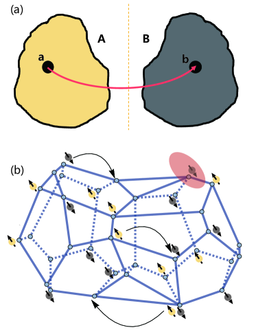
Figure 1: (a) Schematic illustration of the structure of tight-binding model concerned in this work, which supports exceptional spectrum. It consists of two identical sub-systems (two shadow areas A and B, yellow and gray, respectively), which have a reflectional symmetry about the axis (dotted line). Such a system has degeneracy spectrum in the absence of particle-particle interaction. The non-Hermiticity arises from a unidirectional hopping between two symmetric points a and b , which is indicated by the red arrow. It is shown that the non-Hermitian term results in a Jordan block in each subspace spanned by two degenerate states. (b) Schematic of an example system, which is a non-interacting itinerant electron system, described by the Hamiltonian in equation (24). The sub-Hamiltonian for electron with spin up (yellow) corresponds to yellow sub-system in (a), while the spin down (gray) corresponds to the gray part. The non-Hermitian term [red arrow in (a)] is realized by a local critical complex field shaded red.

2 General formalism

In this section, we present a general formalism of systems supporting the coalescing spectrum. Firstly, we construct a class of non-Hermitian Hamiltonians which possesses pseudo-Hermiticity and inversion symmetry. Pseudo-Hermitian Hamiltonian has a real spectrum or else its complex eigenvalues always occur in complex conjugate pairs [75]. A pseudo-Hermitian Hamiltonian satisfies the condition

$$SHS^{-1}=H^{\dagger},$$ (1)

where $S$ is a Hermitian linear automorphism [76]. Secondly, we show that such Hamiltonians can be tuned to have full coalescing spectrum and then support a special dynamics.

2.1 Model and solution

We start with a class of non-Hermitian Hamiltonians in the form

$$H = H_{1}+H_{2}+H_{12},$$ (2)

$$H_{\lambda} = \sum_{i\geqslant j}^{N}J_{ij}a_{i,\lambda}^{{\dagger}}a_{j,\lambda}+\mathrm{H.c.},(\lambda=1,2),$$ (3)

$$H_{12} = \sum_{j=1}^{N}\kappa_{j}a_{j,1}^{{\dagger}}a_{j,2}+\gamma^{2}\sum_{j=1}^{N}\kappa_{j}a_{j,2}^{{\dagger}}a_{j,1},$$ (4)

which consists of two identical Hermitian clusters $H_{\lambda}$ with $\lambda=1,2$, respectively. The structure of the model is schematically illustrated in figure 1(a). The non-Hermiticity arises from the real asymmetrical hopping strength with $\gamma\neq 1$. The distribution of the hopping integrals $\left\{\kappa_{j}\right\}$ determines the non-Hermitian term to be a macroscopic or a local term. Here $a_{j,\lambda}^{{\dagger}}$ ($a_{j,\lambda}$) is the boson or fermion creation (annihilation) operator at the $i$th site in the $\lambda$th cluster. In this work, we only consider unidirectional hopping with the same position for the following reasons: (i) This allows us to perform analytical analysis. (ii) Such a term corresponds to the description of magnetic impurity in the following section. (iii) When the interaction between different positions is considered, the exceptional spectrum may also exists or not, depending on the structure of $H_{\lambda}$, according to the theorem in reference [67]. The cluster $H_{\lambda}$ is defined by the distribution of the hopping integrals $\left\{J_{ij}\right\}$ with $i>j$ and on-site potentials $\left\{J_{jj}\right\}$. The matrix $J_{ij}$ is Hermitian and we only consider the case with $\gamma>0$ in this paper. Two Hamiltonians $H_{\lambda}$ have the same eigenfunctions and real spectral structures and the whole Hamiltonian is not self-adjoint except the case with $\gamma=1$. In the following, we will show that it still has full real spectrum and $\left(N+1\right)$-order exceptional point at $\gamma=0$ (see B), near which the dynamics of the Hamiltonian $H$ is crucial to the conclusion of this paper.

At first, we consider a case with $\gamma=0$ and $\kappa_{j}=\kappa$, representing uniform unidirectional hopping between two identical clusters. The Hermitian Hamiltonians $H_{\lambda}$ can be written in the diagonal form

$$H_{\lambda}=\sum_{k=1}^{N}\varepsilon_{k}A_{k,\lambda}^{{\dagger}}A_{k,\lambda}$$ (5)

by the transformation

$$A_{k,\lambda}=\sum_{j=1}^{N}g_{k,j}a_{j,\lambda},$$ (6)

where we use $k$ to denote the index of eigenmode of $H_{\lambda}$, which becomes wave vector for a system with translational symmetry. Here the spectrum $\varepsilon_{k}$ is real and $g_{k,j}$ satisfies orthonormal relations

$$\sum_{j=1}^{N}\left(g_{k,j}\right)^{\ast}g_{k^{\prime},j}=\delta_{kk^{\prime}},\sum_{k=1}^{N}\left(g_{k,i}\right)^{\ast}g_{k,j}=\delta_{ij},$$ (7)

and can be obtained from the diagonalization of the $N\times N$ matrix $\left\{J_{ij}\right\}$. Accordingly we have

$$H_{12}=\kappa\sum_{j=1}^{N}a_{j,1}^{{\dagger}}a_{j,2}=\kappa\sum_{k=1}^{N}A_{k,1}^{{\dagger}}A_{k,2}$$ (8)

which allows the block diagonal form of the Hamiltonian

$$H = \sum_{k=1}^{N}H_{k}$$ (9)

$$H_{k} = \varepsilon_{k}\left(A_{k,1}^{{\dagger}}A_{k,1}+A_{k,2}^{{\dagger}}A_{k,2}\right)+\kappa A_{k,1}^{{\dagger}}A_{k,2}$$ (10)

$$= \left(\begin{array}[]{ll}A_{k,1}^{{\dagger}}&A_{k,2}^{{\dagger}}\end{array}\right)h_{k}\left(\begin{array}[]{l}A_{k,1}\\ A_{k,2}\end{array}\right).$$ (14)

due to the relation $\left[H_{k},H_{k^{\prime}}\right]=0$. Importantly, matrix

$$h_{k}=\left(\begin{array}[]{ll}\varepsilon_{k}&\kappa\\ 0&\varepsilon_{k}\end{array}\right)$$ (15)

is a Jordan block. The coalescing vector is $\left(\begin{array}[]{ll}1&0\end{array}\right)^{T}$, while the auxiliary vector is $\left(\begin{array}[]{ll}0&1\end{array}\right)^{T}$. Then the eigenstate set of $H$ is identical to that of $H_{1}$, while the auxiliary set is the eigenstate set of $H_{2}$.

Secondly, in the case with nonzero $\gamma$ and non-uniform $\kappa_{j}$, the Hamiltonian can be written as the following form when $H_{\lambda}$ is a bipartite lattice (see A),

$$H=\sum_{n=1,\rho=\pm}^{N}E_{\rho,n}\overline{d}_{n,\rho}d_{n,\rho}.$$ (16)

We note that when taking $\gamma\rightarrow 0$ we have $\overline{d}_{n,\pm}\sim\sum_{j=1}^{N}f_{n,\pm}^{j}a_{j,1}^{{\dagger}}$ and $d_{n,\pm}\sim\sum_{j=1}^{N}\left(f_{n,\pm}^{j}\right)^{\ast}a_{j,2}$, with $f_{n,+}^{j}\longrightarrow f_{n,-}^{j}$, i.e., the pair of operators with subscript $\pm$ coalesce, which accord with the analysis in the case of $\gamma=0$ and $\kappa_{j}=\kappa$. The most fascinating feature of such systems is that even a single unidirectional tunneling (the simplest configuration for non-uniform $\kappa_{j}$) can result in exceptional spectrum.

2.2 Exceptional spectrum and critical dynamics

Now we turn to the dynamics driven by the non-Hermitian Hamiltonian. At first, we still consider a case with $\gamma=0$ and $\kappa_{j}=\kappa$, in which the Hamiltonians $H$ has been written as the sum of $N$ independent sub-Hamiltonians $H_{k}$. In the case of zero $\kappa$, $H$ has two-fold degeneracy spectrum, which is similar to the Kramer’s degeneracy. However, when $\kappa$ is switched on, each pairs of degenerate energy levels coalesce into a single one. The original Kramer’s spectrum transits to an exceptional spectrum. As known that a system at EP exhibits unusual dynamics. It is presumable that a system with exceptional spectrum should supports interesting dynamical phenomena, particularly in many-fermion system.

The dynamics for any initial state is governed by the time evolution operator $U(t)=e^{-iHt}$. It is expressed explicitly as

$$U(t) = \prod_{k}U_{k}(t)=\prod_{k}e^{-iH_{k}t}$$ (17)

$$= e^{-i\sum_{k}\varepsilon_{k}\left(A_{k,1}^{{\dagger}}A_{k,1}+A_{k,2}^{{\dagger}}A_{k,2}\right)t}\prod_{k}e^{-i\kappa A_{k,1}^{{\dagger}}A_{k,2}t}.$$ (18)

For fermion system, we have it reduces to

$$U(t)=\prod_{k}(1-i\kappa A_{k,1}^{{\dagger}}A_{k,2}t),$$ (19)

where an overall dynamical phase factor is omitted and the identity $(A_{k,1}^{{\dagger}}A_{k,2})^{2}=0$ for fermion is used. Then for a given initial state $\left|\Phi(0)\right\rangle=A_{k,2}^{{\dagger}}\left|\mathrm{Vac}\right\rangle$, we have

$$\left|\Phi(t)\right\rangle=\left(A_{k,2}^{{\dagger}}-i\kappa A_{k,1}^{{\dagger}}t\right)\left|\mathrm{Vac}\right\rangle$$ (20)

which indicates $\left|\Phi(\infty)\right\rangle\rightarrow A_{k,1}^{{\dagger}}\left|\mathrm{Vac}\right\rangle$, i.e., transferring an eigenstate of $H_{2}$ to that of $H_{1}$. It can be extended to an arbitrary initial state. We are interested in a typical many-particle initial state

$$\left|\Phi(0)\right\rangle=\prod_{j=1}^{N}a_{j,2}^{{\dagger}}\left|\mathrm{Vac}\right\rangle=\prod_{k}^{N}A_{k,2}^{{\dagger}}\left|\mathrm{Vac}\right\rangle,$$ (21)

which is fully occupied state of system $H_{2}$. In the many-fermion system, high-order exceptional point occurs(see B). Similarly, at large $t$ limit, we have

$$\left|\Phi(t)\right\rangle\propto\prod_{k}^{N}A_{k,1}^{{\dagger}}\left|\mathrm{Vac}\right\rangle=\prod_{j=1}^{N}a_{j,1}^{{\dagger}}\left|\mathrm{Vac}\right\rangle,$$ (22)

i.e., a fully occupied state of system $H_{1}$. We can calculate the number of the fermions in lattice $1$ and $2$

$$n_{\lambda}=\sum_{j=1}^{N}\frac{\left\langle\Phi(t)\right|a_{j,\lambda}^{\dagger}a_{j,\lambda}\left|\Phi(t)\right\rangle}{\left|\left\langle\Phi(t)|\Phi(t)\right\rangle\right|},(\lambda=1,2),$$ (23)

respectively. It indicates that all the fermions in lattice $2$ transfer to lattice $1$, eventually. We find that during the dynamical process, (i) the total particle number is always conservative, (ii) the particle number in lattice $2$ vanishes after sufficient long time for an arbitrary initial state, (iii) it tends to the final state with speed in power law, and the exponent equals to the initial particle number in lattice $2$, the order of EP. Based on these analyses, we conclude that no matter what types of initial state, pure state or mixed state, the final state is a state with a fixed particle number in lattice $1$, which is determined by the maximal particle number in lattice $2$ among all the components of the initial state. For the case with non-uniform $\kappa_{j}$, the solutions we obtained benefit to the numerical simulation for many-fermion system, avoiding the exponentially increasing computer time as a function of the lattice size. We will see that the main result is independent of the distribution of $\left\{\kappa_{j}\right\}$.

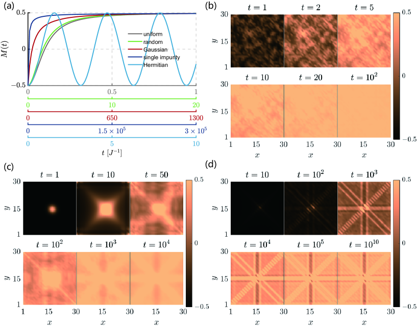
Figure 2: Numerical results for the dynamic magnetization process of a $30\times 30$ square lattice with uniform NN hopping $J_{ij}=J=1$. (a) The average magnetizations $M(t)$ as functions of time for different non-Hermitian field distributions. As a comparison, the result of $M(t)$ for a uniform Hermitian field $\mathbf{B}_{j}=\kappa_{0}(1,0,0)$ is also presented. Panels (b)-(d) are snapshots of the magnetizations $m(x,y,t)$ with three representative non-Hermitian field distributions: random, Gaussian and single impurity, respectively. Other parameters are $\kappa_{0}=1$, $\alpha=0.16$ and $(x_{0},y_{0})=(17,16)$.

3 Dynamic magnetization

In this section we apply the obtained result to a spin-$1/2$ fermionic model with complex impurities [see figure 1(b)]. The Hamiltonian on an arbitrary lattice can be written as

$$H_{\mathrm{F}}=\sum_{i\geqslant j}^{N}\sum_{\sigma=\uparrow,\downarrow}J_{ij}c_{i,\sigma}^{{\dagger}}c_{j,\sigma}+\mathrm{H.c.}+\sum_{j=1}^{N}\mathbf{B}_{j}\cdot\mathbf{s}_{j},$$ (24)

where operator $c_{i,\sigma}^{{\dagger}}$ creates a fermion of spin $\sigma$ at site $i$, and $\mathbf{s}_{j}=(s_{j}^{x},s_{j}^{y},s_{j}^{z})$ is the spin-$1/2$ operator, which is defined by

$$s_{j}^{+} = \frac{1}{2}\left(s_{j}^{x}+is_{j}^{y}\right)=\left(s_{j}^{-}\right)^{{\dagger}}=c_{j,\uparrow}^{{\dagger}}c_{j,\downarrow}$$ (25)

$$s_{j}^{z} = \frac{1}{2}\left(c_{j,\uparrow}^{{\dagger}}c_{j,\uparrow}-c_{j,\downarrow}^{{\dagger}}c_{j,\downarrow}\right)$$ (26)

satisfying the Lie algebra commutation relations,

$$\left[s^{+},s^{-}\right]=2s^{z},\left[s^{z},s^{\pm}\right]=\pm s^{\pm}.$$ (27)

Here $J_{ij}$ for $i\neq j$ is hopping strength between two sites ($i,j$), and $J_{jj}$ is on-site potential. $\mathbf{B}_{j}$ is on-site complex magnetic field, inducing non-Hermitian impurities. The motivation of introducing a complex magnetic field is to simulating the classical magnetization process in the framework of quantum mechanics. As well known, the friction must be involved in the theory of magnetization based on the classical physics. Non-Hermitian Hamiltonian with a complex magnetic field may be a good candidate for this task.

In history, a complex field was usually induced to characterize the connections between a closed system to the environment phenomenologically. Recently, the topic of complex field has been investigated from many aspects.Theoretically, a non-Hermitian Hamiltonian is the reduced description for a selected sub-system of a Hermitian system, where the complementary subspace is take into account by means of an effective interaction described by a non-Hermitian complex potential [77, 24, 78]. Experimentally, a complex field is usually simulated in the optical system with gain and loss [79, 80, 81]. In addition, there is an experimental protocol for complex magnetic field via atomic system, referred to as ”heralded Magnetism”[82]. Very recently, the non-Hermiticity in real quantum systems has been experimentally demonstrated [83, 84, 85, 86, 87].

In this work, we only consider the field in the form

$$\mathbf{B}_{j}=\kappa_{j}(1,i,0),$$ (28)

with several typical distribution of $\left\{\kappa_{j}\right\}$. $B_{j}\cdot s_{j}$ is the non-Hermitian term. It can drive the fermion from spin-down state $c_{j,\downarrow}^{{\dagger}}\left|\mathrm{Vac}\right\rangle$ to the spin-up state $c_{j,\uparrow}^{{\dagger}}\left|\mathrm{Vac}\right\rangle$ at $j$-th site. The crucial point is that the local system $\mathbf{B}_{j}\cdot\mathbf{s}_{j}$ is at EP. Remarkably, the result in above section tells us that it may induce multi-EP of the whole system. The fermionic Hamiltonian $H_{\mathrm{F}}$ can be expressed in the form of $H$ in equation (2) by taking $c_{j,\uparrow}=a_{j,1}$ and $c_{j,\downarrow}=a_{j,2}$, respectively. Accordingly, the inversion operator $\mathcal{P}$ (see A) maps to spin-reversal operator $\mathcal{S}$, where $\mathcal{S}$ has the action $\mathcal{S}c_{j,\sigma}^{{\dagger}}$($c_{j,\sigma}$)$\mathcal{S}^{-1}=c_{j,-\sigma}^{{\dagger}}$($c_{j,-\sigma}$). A straightforward result can be obtained from the analysis in last section.

We are interested in the dynamic process of magnetization driven by non-Hermitian magnetic field. We first consider the simplest case with uniform field distribution $\mathbf{B}_{j}=\kappa(1,i,0)$. The system we concern is half-filled and the initial state is a saturated ferromagnetic state

$$\left|\Phi(0)\right\rangle=\left|\Downarrow\right\rangle=\prod_{j=1}^{N}c_{j,\downarrow}^{{\dagger}}\left|\mathrm{Vac}\right\rangle,$$ (29)

which is a popular state in physics. Here we choose this initial state for the convenience of calculation. The evolved state driven by the Hamiltonian with non-Hermitian magnetic field is

$$\left|\Phi(t)\right\rangle=\prod_{k=1}^{N}(1-i\kappa C_{k,\uparrow}^{{\dagger}}C_{k,\downarrow}t)\prod_{j=1}^{N}c_{j,\downarrow}^{{\dagger}}\left|\mathrm{Vac}\right\rangle,$$ (30)

which shows that the amplitude of the evolved state is dominant by the term with $t^{N}$ for a long time. Here an overall dynamical phase factor is omitted and

$$C_{k,\sigma}=\sum_{j=1}^{N}g_{k,j}c_{j,\sigma}.$$ (31)

We employ magnetization

$$m_{j}(t)=\frac{\left\langle\Phi(t)\right|s_{j}^{z}\left|\Phi(t)\right\rangle}{\left|\left|\Phi(t)\right\rangle\right|^{2}},$$ (32)

and average magnetization

$$M(t)=\frac{1}{N}\sum_{j=1}^{N}m_{j}(t),$$ (33)

to characterize the dynamic magnetization process. Based on the identity

$$\prod_{j=1}^{N}c_{j,\downarrow}^{{\dagger}}\left|\mathrm{Vac}\right\rangle=\prod_{k=1}^{N}C_{k,\downarrow}^{{\dagger}}\left|\mathrm{Vac}\right\rangle,$$ (34)

which are two expressions of a same state with fully filled spin-up electrons, in real space and collective mode space, respectively. a straightforward derivation results in

$$M\left(t\right)=\frac{\sum_{n=0}^{N}(2n-N)C_{N}^{n}(\kappa t)^{2n}}{\left(2N\right)\sum_{n=0}^{N}C_{N}^{n}(\kappa t)^{2n}}=\frac{(\kappa t)^{2}-1}{2\left[(\kappa t)^{2}+1\right]},$$ (35)

$M\left(t\right)$ is plotted in figure 2(a), in comparison with numerical results for various situations. It is clear that after a long time, $\left|\Phi(t)\right\rangle$ tends to another saturated ferromagnetic state

$$\left|\Uparrow\right\rangle=\prod_{k=1}^{N}C_{k,\uparrow}^{{\dagger}}\left|\mathrm{Vac}\right\rangle=\prod_{j=1}^{N}c_{j,\uparrow}^{{\dagger}}\left|\mathrm{Vac}\right\rangle,$$ (36)

with $M\left(\infty\right)=1/2$. In fact, no matter what the initial state is, after a long time, the evolved state tends to the state in equation (36) due to the EP dynamics.

It is interesting to investigate what happens when $\left\{\kappa_{j}\right\}$ is taken as non-uniform distributions in two-dimensional(2D) square lattice with uniform nearest neighbor (NN) $\left\langle i,j\right\rangle$ hopping strength $J_{ij}=1$. Numerical simulations are performed for three typical forms: (i) Random distribution $\kappa(x,y)=\kappa_{0}\mathrm{Ran}[0,1]$, where Ran$[0,1]$ denotes uniform random real number within the interval $[0,1]$, (ii) Gaussian distribution $\kappa(x,y)=\kappa_{0}\exp\{-\alpha^{2}[(x-x_{0})^{2}+(y-y_{0})^{2}]\}$, and (iii) Single impurity $\kappa(x,y)=\kappa_{0}\delta(x-x_{0})\delta(y-y_{0})$. Numerical simulations for the dynamical processes of magnetization are performed for such three representative cases. Numerical results for $M(t)$ and $m(x,y,t)=m_{j}(t)$ [the coordinate of position $j$ in 2D square lattice is $(x,y)$] are plotted in figure 2(a) and figure 2(b)-2(d), respectively. We find that the itinerant electron system with different distributions of non-Hermitian magnetic field have similar dynamical processes and all tend to the same saturated ferromagnetic state $\left|\Uparrow\right\rangle=\prod_{j=1}^{N}c_{j,\uparrow}^{{\dagger}}\left|\mathrm{Vac}\right\rangle$ with $M\left(\infty\right)=1/2$ finally. In contrast, for the case of uniform Hermitian field, $M(t)$ is a periodic function. To measure the speed of the magnetization we introduce a dimensionless quantity $\mathrm{N}\left(t\right)$

$$\mathrm{N}\left(t\right)=\ln\frac{1+2M\left(t\right)}{1-2M\left(t\right)}.$$ (37)

From equation (35), we find that for the case with uniform field distribution we simply have $\mathrm{N}\left(t\right)=2\ln\kappa+2\ln t$, where factor $2$ characterize the speed. $\mathrm{\ N}(t)$ for the processes in figure 2 are plotted in figure 3(a). It shows that the final results are independent of the distributions of $\kappa(x,y)$, which only affects the speed of the magnetization. Figure 3(b) indicates that for a smaller $\kappa_{0}$, the speed of magnetization is closer to that of uniform field distribution. We also investigate the effect of dimensionality on the speed of the magnetization. We compute $\mathrm{N}(t)$ for several typical cases, including $1$D periodic chain, $2$D square lattice and $3$D cubic lattice with single non-Hermitian impurity [see figure 3(c)]. It indicates that the result is independent of the dimensionality approximately.

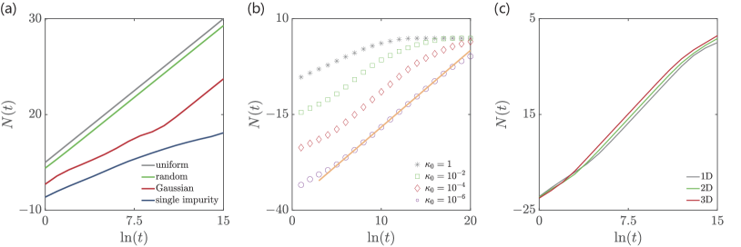
Figure 3: Plots of $\mathrm{N}(t)$ defined in equation (37) as functions of $\ln(t)$. (a) $\mathrm{N}(t)$ for a $30\times 30$ square lattice with different non-Hermitian field distributions, which correspond to the processes plotted in figure 2(a). (b) $\mathrm{N}(t)$ for a $20\times 20$ square lattice with single impurity $\kappa_{0}\delta(x-11)\delta(y-10)$ under different field strength $\kappa_{0}$. The orange line is $\mathrm{N}(t)=2\ln t-38.2$, which indicates that for a smaller $\kappa_{0}$, the speed of magnetization is closer to that of uniform field distribution. (c) $\mathrm{N}(t)$ for the lattices of different dimension (1D, 2D and 3D) with single impurity of field strength $\kappa_{0}=1$. The size of three lattices are $64$, $8\times 8$, and $4\times 4\times 4$, The positions of the impurity of the 2D and 3D lattices are $(4,1)$ and $(2,3,1)$, respectively.

4 Summary

In summary, we have developed a theory for a class of non-Hermitian Hamiltonian which supports a special dynamics due to the appearance of exceptional full real spectrum. The most fascinating feature of such systems is that even a single unidirectional tunneling can result in exceptional spectrum. It is shown that a macroscopic effect can be induced by a local interaction in a non-Hermitian system. To demonstrate this point, we apply the theory on an itinerant electron system subjected to complex fields. As an application, we have studied the dynamic magnetization induced by the field. It shows that an initial saturated ferromagnetic state at half-filling can be driven into its opposite state according to the dynamics of high-order exceptional point. Numerical simulations for several representative situations, including lattice dimensions, global random and local impurity distributions indicate that the dynamic magnetization processes exhibit universal behavior. Our findings provide alternative explanation for dynamic magnetization process in itinerant electron systems in the context of non-Hermitian quantum mechanics.

Appendix A The derivations of the Hamiltonian and the coalescing spectrum

In this Appendix, we present a derivation on the solution of the Hamiltonian $H$ in equation (2) on a bipartite lattice with nonzero $\gamma$ and show that the coalescing spectrum appears as $\gamma$ truns to zero.

To this end, we introduce a set of particle operators $\overline{d}_{j,\lambda}$ and $d_{j,\lambda}$ [43].

$$\overline{d}_{j,1} = \frac{1}{\sqrt{\gamma}}a_{j,1}^{{\dagger}},d_{j,1}=\sqrt{\gamma}a_{j,1},$$ (A 1)

$$\overline{d}_{j,2} = \sqrt{\gamma}a_{j,2}^{{\dagger}},d_{j,2}=\frac{1}{\sqrt{\gamma}}a_{j,2},$$ (A 2)

which are canonical conjugate pairs, satisfying

$$[d_{j,\lambda},\overline{d}_{i,\lambda^{\prime}}]_{\pm} = \delta_{ij}\delta_{\lambda\lambda^{\prime}},$$ (A 3)

$$[d_{j,\lambda},d_{i,\lambda^{\prime}}]_{\pm} = [\overline{d}_{j,\lambda},\overline{d}_{i,\lambda^{\prime}}]_{\pm}=0,$$ (A 4)

where $[\cdot,\cdot]_{\pm}$ denotes the commutator and anti-commutator. Transformation in equation (A 2) is essentially a similarity transformation with a singularity at $\gamma=0$, beyond which it allows us to rewrite the Hamiltonians in the form

$$H_{\lambda} = \sum_{i\geqslant j}^{N}J_{ij}\overline{d}_{i,\lambda}d_{j,\lambda}+\sum_{i\geqslant j}^{N}\left(J_{ij}\right)^{\ast}\overline{d}_{j,\lambda}d_{i,\lambda}$$ (A 5)

$$H_{12} = \gamma\sum_{j=1}^{N}\kappa_{j}\overline{d}_{i,1}d_{j,2}+\gamma\sum_{j=1}^{N}\left(\kappa_{j}\right)^{\ast}\overline{d}_{j,2}d_{i,1}.$$ (A 6)

More explicitly we have

$$H=\sum_{i,j=1}^{N}\sum_{\lambda,\lambda^{\prime}=1}^{2}\overline{d}_{i,\lambda}\mathcal{H}_{i,j,\lambda,\lambda^{\prime}}d_{j,\lambda^{\prime}},$$ (A 7)

where the core matrix is

$$\mathcal{H} = \sum_{i\geqslant j}^{N}\sum_{\lambda=1,2}J_{ij}\left|i,\lambda\right\rangle\overline{\left\langle j,\lambda\right|}+\sum_{i\geqslant j}^{N}\sum_{\lambda=1,2}\left(J_{ij}\right)^{\ast}\left|j,\lambda\right\rangle\overline{\left\langle i,\lambda\right|}$$ (A 9)

$$+\gamma\sum_{j=1}^{N}\kappa_{j}\left|j,1\right\rangle\overline{\left\langle j,2\right|}+\gamma\sum_{j=1}^{N}\left(\kappa_{j}\right)^{\ast}\left|j,2\right\rangle\overline{\left\langle j,1\right|}.$$

based on the orthonormal complete basis $\left\{\left|i,\lambda\right\rangle\right\}=\left\{\overline{d}_{i,\lambda}\left|\mathrm{\ Vac}\right\rangle\right\}$and $\left\{\overline{\left\langle i,\lambda\right|}\right\}=\left\{\left\langle\mathrm{Vac}\right|d_{i,\lambda}\right\}$($\left|\mathrm{Vac}\right\rangle$ is the vacuum state of operator $a_{j,\lambda}$), satisfying

$$\overline{\left\langle i,\lambda\right|}j,\lambda^{\prime}\rangle=\delta_{ij}\delta_{\lambda\lambda^{\prime}}.$$ (A 10)

We find that the matrix $\mathcal{H}$ is Hermitian in the basis set $\left\{\left|i,\lambda\right\rangle,\overline{\left\langle i,\lambda\right|}\right\}$, although $\left(\left|i,\lambda\right\rangle\right)^{{\dagger}}\neq\overline{\left\langle i,\lambda\right|}$. For the sake of simplicity, we only need to diagonalize such a Hermitian matrix

$$h=\sum_{i\geqslant j}^{N}\sum_{\lambda=1,2}J_{ij}\left|i,\lambda\right\rangle\left\langle j,\lambda\right|+\gamma\sum_{j=1}^{N}\kappa_{j}\left|j,1\right\rangle\left\langle j,2\right|+\mathrm{H.c.},$$ (A 11)

with $\left\langle i,\lambda\right|j,\lambda^{\prime}\rangle=\delta_{ij}\delta_{\lambda\lambda^{\prime}}.$ Importantly, $h$ has inversion symmetry due to the reality of matrix elements $\left\{\kappa_{j}\right\}$, i.e.,

$$\mathcal{P}h\mathcal{P}^{-1}=h,$$ (A 12)

where $\mathcal{P}$ has the action $\mathcal{P}\left|j,1\right\rangle=\left|j,2\right\rangle$ ($\mathcal{P}\left|j,2\right\rangle=\left|j,1\right\rangle$). Note that such symmetry is independent of the structure of the sub-lattice determined by $\left\{J_{ij}\right\}$. Then we can rewrite the matrix in the block diagonal form

$$h=h_{+}+h_{-},$$ (A 13)

where

$$h_{\pm}=\sum_{i\geqslant j}^{N}J_{ij}\left|i,\pm\right\rangle\left\langle j,\pm\right|+\mathrm{H.c.}\pm\gamma\sum_{j=1}^{N}\kappa_{j}\left|j,\pm\right\rangle\left\langle j,\pm\right|,$$ (A 14)

and

$$\left|j,\pm\right\rangle=\frac{\left|j,1\right\rangle\pm\left|j,2\right\rangle}{\sqrt{2}}.$$ (A 15)

We note that $h_{+}$ and $h_{-}$ satisfy $\left[h_{+},h_{-}\right]=0$ and the matrice of $h_{+}$ and $h_{-}$ become identical as $\gamma\rightarrow 0$. Accordingly, the solution of the Schrodinger equation

$$h_{\pm}\left|\psi_{\pm,n}\right\rangle=E_{\pm,n}\left|\psi_{\pm,n}\right\rangle,$$ (A 16)

has the form

$$\left|\psi_{\pm,n}\right\rangle=\sum_{j=1}^{N}f_{n,\pm}^{j}\frac{\left|j,1\right\rangle\pm\left|j,2\right\rangle}{\sqrt{2}},$$ (A 17)

satisfying

$$\mathcal{P}\left|\psi_{\pm,n}\right\rangle=\pm\left|\psi_{\pm,n}\right\rangle.$$ (A 18)

Then the Hamiltonian is diagonalized as the form

$$H=\sum_{n=1,\rho=\pm}^{N}E_{\rho,n}\overline{d}_{n,\rho}d_{n,\rho},$$ (A 19)

where

$$\overline{d}_{n,\pm} = \sum_{j=1}^{N}f_{n,\pm}^{j}\left(\frac{1}{\sqrt{\gamma}}a_{j,1}^{{\dagger}}\pm\sqrt{\gamma}a_{j,2}^{{\dagger}}\right),$$ (A 20)

$$d_{n,\pm} = \sum_{j=1}^{N}\left(f_{n,\pm}^{j}\right)^{\ast}\left(\sqrt{\gamma}a_{j,1}\pm\frac{1}{\sqrt{\gamma}}a_{j,2}\right).$$ (A 21)

Although the above solution is only true for nonzero $\gamma$, one can extrapolate the approximate solution at $\gamma=0$ by taking $\gamma\rightarrow 0$. In the limit of zero $\gamma$, we have $f_{n,+}^{j}\longrightarrow f_{n,-}^{j}\rightarrow g_{k,j}$, which results in

$$\overline{d}_{n,\pm}\sim\sum_{j=1}^{N}g_{k,j}a_{j,1}^{{\dagger}},d_{n,\pm}\sim\sum_{j=1}^{N}\left(g_{k,j}\right)^{\ast}a_{j,2}.$$ (A 22)

We demonstrate the result by a simple system, which consists of two identical $N$-site uniform chain with a unidirectional hopping between them. The Hamiltonian has the form

$$H = H_{1}+H_{2}+H_{12},$$ (A 23)

$$H_{\lambda} = \sum_{i=1}^{N-1}Ja_{i,\lambda}^{\dagger}a_{i+1,\lambda}+\mathrm{H.c.},(\lambda=1,2)$$ (A 24)

$$H_{12} = \kappa a_{1,1}^{\dagger}a_{1,2}.$$ (A 25)

According to our analysis above, the eigenvalues and eigenvectors in single-particle invariant subspace have the form

$$\epsilon_{1,n} = 2J\cos\left(\frac{n\pi}{N+1}\right),$$ (A 26)

$$\left|\psi_{1,n}\right\rangle = \sqrt{\frac{2}{N+1}}\sum_{j=1}^{N}\sin\left(\frac{n\pi}{N+1}j\right)a_{j,1}^{\dagger}\left|\mathrm{Vac}\right\rangle,$$ (A 27)

which satisfies

$${H}\left|\psi_{1,n}\right\rangle=\epsilon_{1,n}\left|\psi_{1,n}\right\rangle.$$ (A 28)

Similarly, for the system ${H}^{{\dagger}}$, we have

$$\left|\varphi_{1,n}\right\rangle=\sqrt{\frac{2}{N+1}}\sum_{j=1}^{N}\sin\left(\frac{n\pi}{N+1}j\right)a_{j,2}^{\dagger}\left|\mathrm{Vac}\right\rangle,$$ (A 29)

which satisfies

$${H}^{{\dagger}}\left|\varphi_{1,n}\right\rangle=\epsilon_{1,n}\left|\varphi_{1,n}\right\rangle.$$ (A 30)

Obviously we have

$$\langle\varphi_{1,m}\left|\psi_{1,n}\right\rangle=0,$$ (A 31)

for any $m$ and $n$, which indicates that $\left|\psi_{1,n}\right\rangle$ is coalscing states due to the vanishing biorthogonal norm [10]. Furthermore, this conclusion can be true for the case with multiple unidirectional hoppings.

Appendix B High-order exceptional point

In this Appendix, we prove that our system with more than one fermion has high-order exceptional point.

We consider the following case. In the $N$-fermion invariant subspace with each $k$ filled by one fermion. In this $N$-fermion basis, the matrix representation of Hamiltonian $H$ in equation (14) can be written as

$$h=T_{N}+\sum_{k=1}^{N}\varepsilon_{k}.$$ (B 1)

Here $T_{N}$ can be expressed in the form

$$T_{N} = I_{2}\otimes T_{N-1}+T_{1}\otimes I_{2^{N-1}}$$ (B 2)

$$= \left(\begin{array}[]{cc}T_{N-1}&\kappa I_{2^{N-1}}\\ \mathbf{0}&T_{N-1}\end{array}\right),$$ (B 5)

$$T_{1} = \left(\begin{array}[]{cc}0&\kappa\\ 0&0\end{array}\right),$$ (B 8)

which means that after the Jordan decomposition, the size of the largest Jordan block of $T_{N}$ is $1$ larger than that of $T_{N-1}$. Because $T_{1}$ is a $2$-order Jordan block, the largest Jordan block of $h$ is $\left(N+1\right)$-order, which means that the $N$-fermion system has exceptional point of $\left(N+1\right)$-order.

References

- [1] Musslimani Z, Makris K G, El-Ganainy R and Christodoulides D N 2008 Physical Review Letters 100 030402
- [2] Makris K G, El-Ganainy R, Christodoulides D and Musslimani Z H 2008 Physical Review Letters 100 103904
- [3] Klaiman S, Günther U and Moiseyev N 2008 Physical review letters 101 080402
- [4] Rüter C E, Makris K G, El-Ganainy R, Christodoulides D N, Segev M and Kip D 2010 Nature physics 6 192–195
- [5] Chong Y, Ge L, Cao H and Stone A D 2010 Physical review letters 105 053901
- [6] Regensburger A, Bersch C, Miri M A, Onishchukov G, Christodoulides D N and Peschel U 2012 Nature 488 167–171
- [7] Feng L, Xu Y L, Fegadolli W S, Lu M H, Oliveira J E, Almeida V R, Chen Y F and Scherer A 2013 Nature materials 12 108–113
- [8] Fleury R, Sounas D and Alù A 2015 Nature communications 6 1–7
- [9] Bender C M 2007 Reports on Progress in Physics 70 947
- [10] Moiseyev N 2011 Non-Hermitian quantum mechanics (Cambridge University Press)
- [11] Feng L, El-Ganainy R and Ge L 2017 Nature Photonics 11 752–762
- [12] El-Ganainy R, Makris K G, Khajavikhan M, Musslimani Z H, Rotter S and Christodoulides D N 2018 Nature Physics 14 11–19
- [13] Gupta S K, Zou Y, Zhu X Y, Lu M H, Zhang L J, Liu X P and Chen Y F 2020 Advanced Materials 32 1903639
- [14] Christodoulides D, Yang J et al. 2018 Parity-time symmetry and its applications vol 280 (Springer)
- [15] Znojil M 2007 Physics Letters B 650 440–446
- [16] Znojil M 2007 Journal of Physics A: Mathematical and Theoretical 40 13131
- [17] Bendix O, Fleischmann R, Kottos T and Shapiro B 2009 Physical Review Letters 103 030402
- [18] Longhi S 2009 Physical review letters 103 123601
- [19] Longhi S 2009 Physical Review B 80 235102
- [20] Jin L and Song Z 2009 Physical Review A 80 052107
- [21] Znojil M 2010 Physical Review A 82 052113
- [22] Longhi S 2010 Physical Review B 81 195118
- [23] Longhi S 2010 Physical Review B 82 041106
- [24] Jin L and Song Z 2010 Physical Review A 81 032109
- [25] Joglekar Y N, Scott D, Babbey M and Saxena A 2010 Physical Review A 82 030103
- [26] Znojil M 2011 Journal of Physics A: Mathematical and Theoretical 44 075302
- [27] Znojil M 2011 Physics Letters A 375 3176–3183
- [28] Zhong H, Hai W, Lu G and Li Z 2011 Physical Review A 84 013410
- [29] Drissi L, Saidi E and Bousmina M 2011 Journal of mathematical physics 52 022306
- [30] Joglekar Y N and Saxena A 2011 Physical Review A 83 050101
- [31] Scott D D and Joglekar Y N 2011 Physical Review A 83 050102
- [32] Joglekar Y N and Barnett J L 2011 Physical Review A 84 024103
- [33] Scott D D and Joglekar Y N 2012 Physical Review A 85 062105
- [34] Lee T E and Joglekar Y N 2015 Physical Review A 92 042103
- [35] Kulishov M, Laniel J M, Bélanger N, Azaña J and Plant D V 2005 Optics express 13 3068–3078
- [36] Longhi S 2010 Optics letters 35 3844–3846
- [37] Lin Z, Ramezani H, Eichelkraut T, Kottos T, Cao H and Christodoulides D N 2011 Physical Review Letters 106 213901
- [38] Eichelkraut T, Heilmann R, Weimann S, Stützer S, Dreisow F, Christodoulides D N, Nolte S and Szameit A 2013 Nature communications 4 1–7
- [39] Eichelkraut T, Heilmann R, Weimann S, Stützer S, Dreisow F, Christodoulides D N, Nolte S and Szameit A 2013 Nature communications 4 1–7
- [40] Chang L, Jiang X, Hua S, Yang C, Wen J, Jiang L, Li G, Wang G and Xiao M 2014 Nature photonics 8 524–529
- [41] Longhi S 2010 Physical Review A 82 032111
- [42] Longhi S and Della Valle G 2013 Annals of Physics 334 35–46
- [43] Zhang X and Song Z 2013 Annals of Physics 339 109–121
- [44] Jin L and Song Z 2021 Chinese Physics Letters 38 024202
- [45] Sun Y, Tan W, Li H q, Li J and Chen H 2014 Physical review letters 112 143903
- [46] Mostafazadeh A 2009 Physical review letters 102 220402
- [47] Longhi S 2009 Physical Review B 80 165125
- [48] Zhang X, Jin L and Song Z 2013 Physical Review A 87 042118
- [49] Longhi S 2015 Optics letters 40 5694–5697
- [50] Li X, Zhang X, Zhang G and Song Z 2015 Physical Review A 91 032101
- [51] Jin L 2017 Physical Review A 96 032103
- [52] Peng B, Özdemir Ş, Rotter S, Yilmaz H, Liertzer M, Monifi F, Bender C, Nori F and Yang L 2014 Science 346 328–332
- [53] Feng L, Wong Z J, Ma R M, Wang Y and Zhang X 2014 Science 346 972–975
- [54] Hodaei H, Hayenga W, Miri M A, Hassan A, Christodoulides D and Khajavikhan M 2015 Tunable parity-time-symmetric microring lasers CLEO: Science and Innovations (Optical Society of America) pp SF1I–1
- [55] Jin L and Song Z 2018 Physical Review Letters 121 073901
- [56] Krasnok A, Baranov D, Li H, Miri M A, Monticone F and Alú A 2019 Advances in Optics and Photonics 11 892–951
- [57] Doppler J, Mailybaev A A, Böhm J, Kuhl U, Girschik A, Libisch F, Milburn T J, Rabl P, Moiseyev N and Rotter S 2016 Nature 537 76–79
- [58] Xu H, Mason D, Jiang L and Harris J 2016 Nature 537 80–83
- [59] Assawaworrarit S, Yu X and Fan S 2017 Nature 546 387–390
- [60] Midya B, Zhao H and Feng L 2018 Nature communications 9 1–4
- [61] Cao S and Hou Z 2019 Physical Review Applied 12 064016
- [62] Miri M A and Alù A 2019 Science 363 eaar7709
- [63] Miao P, Zhang Z, Sun J, Walasik W, Longhi S, Litchinitser N M and Feng L 2016 Science 353 464–467
- [64] Longhi S and Feng L 2017 Photonics Research 5 B1–B6
- [65] Chen W, Kaya Özdemir Ş, Zhao G, Wiersig J and Yang L 2017 Nature 548 192–196
- [66] Hodaei H, Hassan A U, Wittek S, Garcia-Gracia H, El-Ganainy R, Christodoulides D N and Khajavikhan M 2017 Nature 548 187–191
- [67] Wang P, Zhang K and Song Z 2021 Physical Review B 104 245406
- [68] Wang P, Zhang K and Song Z 2020 Physical Review A 101 022111
- [69] Zhang X Z, Jin L and Song Z 2020 Phys. Rev. B 101(22) 224301
- [70] Zhang S, Zhang X, Jin L and Song Z 2020 Physical Review A 101 033820
- [71] Hodaei H, Hassan A U, Wittek S, Garcia-Gracia H, El-Ganainy R, Christodoulides D N and Khajavikhan M 2017 Nature 548 187–191
- [72] Schnabel J, Cartarius H, Main J, Wunner G and Heiss W D 2017 arXiv preprint arXiv:1708.03206
- [73] Ding K, Ma G, Xiao M, Zhang Z and Chan C T 2016 Physical Review X 6 021007
- [74] Jin L 2018 Physical Review A 97 012121
- [75] Mostafazadeh A 2002 Journal of Mathematical Physics 43 205–214
- [76] Sundar Mukherjee S and Roy P 2014 arXiv e-prints arXiv–1401
- [77] Muga J, Palao J, Navarro B and Egusquiza I 2004 Physics Reports 395 357–426
- [78] Jin L and Song Z 2011 Journal of Physics A: Mathematical and Theoretical 44 375304
- [79] Gupta S K, Zou Y, Zhu X Y, Lu M H, Zhang L J, Liu X P and Chen Y F 2020 Advanced Materials 32 1903639
- [80] Guo A, Salamo G, Duchesne D, Morandotti R, Volatier-Ravat M, Aimez V, Siviloglou G and Christodoulides D 2009 Physical review letters 103 093902
- [81] Makris K G, El-Ganainy R, Christodoulides D and Musslimani Z H 2008 Physical Review Letters 100 103904
- [82] Lee T E and Chan C K 2014 Physical Review X 4 041001
- [83] Ren Z, Liu D, Zhao E, He C, Pak K K, Li J and Jo G B 2022 Nature Physics 18 385–389
- [84] Liu W, Wu Y, Duan C K, Rong X and Du J 2021 Physical Review Letters 126 170506
- [85] Wu Y, Liu W, Geng J, Song X, Ye X, Duan C K, Rong X and Du J 2019 Science 364 878–880
- [86] Partanen M, Goetz J, Tan K Y, Kohvakka K, Sevriuk V, Lake R E, Kokkoniemi R, Ikonen J, Hazra D, Mäkinen A et al. 2019 Physical Review B 100 134505
- [87] Li J, Harter A K, Liu J, de Melo L, Joglekar Y N and Luo L 2019 Nature communications 10 1–7