Assessing the validity of Bayesian inference using loss functions

Abstract

In the usual Bayesian setting, a full probabilistic model is required to link the data and parameters, and the form of this model and the inference and prediction mechanisms are specified via de Finetti’s representation. In general, such a formulation is not robust to model mis-specification of its component parts. An alternative approach is to draw inference based on loss functions, where the quantity of interest is defined as a minimizer of some expected loss, and to construct posterior distributions based on the loss-based formulation; this strategy underpins the construction of the Gibbs posterior. We develop a Bayesian non-parametric approach; specifically, we generalize the Bayesian bootstrap, and specify a Dirichlet process model for the distribution of the observables. We implement this using direct prior-to-posterior calculations, but also using predictive sampling. We also study the assessment of posterior validity for non-standard Bayesian calculations, and provide an efficient way to calibrate the scaling parameter in the Gibbs posterior so that it can achieve the desired coverage rate. We show that the developed non-standard Bayesian updating procedures yield valid posterior distributions in terms of consistency and asymptotic normality under model mis-specification. Simulation studies show that the proposed methods can recover the true value of the parameter efficiently and achieve frequentist coverage even when the sample size is small. Finally, we apply our methods to evaluate the causal impact of speed cameras on traffic collisions in England.

Key words: General Bayesian updating; Loss functions; Bayesian predictive inference; Scaling parameter; Semi-parameter inference

1 Introduction and motivation

Bayesian inference methods are central to decision making under uncertainty. The most common approach to Bayesian (prior-to-posterior) updating employs parametric specifications of probability models for the observable quantities, but there has also been much research on relaxing parametric assumptions, as parametric models are not typically robust to model mis-specification; that is, they rely on correct specification of (at least) the likelihood that appears in de Finetti’s representation. In standard prior-to-posterior inference, coherent Bayesian updating of prior beliefs on the parameter follows from an assumption of exchangeability of the observable quantities, the de Finetti representation for the corresponding probability model, and the combination of prior distribution on the unobservable data generating model with an induced conditional probability model for the observables. In contrast, Zhang (2006), Jiang and Tanner (2008), and Bissiri et al. (2016) adopt a decision-making approach, and formulate posterior inference entirely on a loss (or utility) specification to target a specific parameter in the data-generating distribution, leading to the so-called Gibbs posterior. The Gibbs posterior results from a prior-to-posterior update where the loss function is converted to yield a pseudo-likelihood, and then combined with a prior distribution. An advantage of the targeting of a specific parameter of interest is that a full probabilistic specification for the data generating model for the observables is avoided. However, a disadvantage is that in general a probabilistic interpretation of the assumptions concerning the distribution of the observables is lost. In this paper, we explore the probabilistic validity of inference based purely on loss functions.

1.1 Parameter definition

Common to both standard Bayesian inference and the Gibbs posterior approach is that the quantities of interest are expressed as some functional of the data generating process, which is characterized by the distribution $F^{\ast}$. In any inference problem, $F^{\ast}$ – and thus any functional of it – is regarded as unknown quantity, and uncertainty is present due to absence of perfect knowledge of $F^{\ast}$. If prior uncertainty for $F^{\ast}$ is encapsulated in a prior distribution, the form of the posterior on $F^{\ast}$, and the posterior of any parameter of interest, can be deduced.

In the standard Bayesian approach, a ‘parameter’ is defined as a functional of the limiting distribution of the exchangeable observables. In a parametric specification, $F^{\ast}(z)\equiv F^{\ast}(z|\xi^{\ast})$, where $\xi^{\ast}$ lies in the finite dimensional parameter space $\Xi$. In the simplest case of exchangeable binary variables $\{Z_{i},i=1,\ldots,n,\ldots\}$, for any $n\geq 1$, we have that for any binary sequence $z_{1},\ldots,z_{n}$, the joint distribution can be written using the de Finetti representation as the integral over ‘parameter’ $\xi$ of the product of the conditional densities $f^{\ast}(z_{i}|\xi)=\xi^{z_{i}}(1-\xi)^{1-{z_{i}}}$ and prior $\pi_{0}(\xi)$, where the true (data generating) parameter and distribution coincide with

$$\xi^{\ast}=\lim_{n\longrightarrow\infty}\frac{1}{n}\sum_{i=1}^{n}Z_{i}\quad\text{and}\quad F^{\ast}((-\infty,z])=\lim_{n\longrightarrow\infty}\frac{1}{n}\sum_{i=1}^{n}\mathbb{1}_{(-\infty,z]}(Z_{i})\quad z\in\mathbb{R}$$

respectively. The de Finetti representation defines ‘parameters’ in this way, although definitions based on invariance, sufficiency, and information can also be used – see Bernardo and Smith (1994, Chap.4).

A formulation that identifies the same parameter is based on loss minimization, with

$$\xi^{\ast}=\arg\min_{t}\int-\log f^{\ast}(z|t)dF^{\ast}(z)=\arg\max_{t}\int(z\log t+(1-z)\log(1-t))dF^{\ast}(z).$$

The loss function $\ell(z,t)=-\log f^{\ast}(z|t)$ defines the parameter as that which minimizes the expected loss under $F^{\ast}(z|\xi^{\ast})$.

Note that we may equivalently define $\xi^{\ast}$ via a different loss function and functional of $F^{\ast}$: for example, using $\ell(z,t)=\lambda(z-t)^{2}$ with parameter $\lambda>0$ returns the same minimizer, so the formulation via a loss function minimization is not unique. This is not problematic per se, and illustrates the importance of ‘modelling’ the connection between observables and the parameter. However, there is no equivalent de Finetti representation in the second formulation, as this would require $-\log f^{\ast}(z|t)=\lambda(z-t)^{2}+h(z)$ for some function $h(z)$ that does not depend on $t$, so that $f^{\ast}(z|t)=\exp\{-\lambda(z-t)^{2}-h(z)\}$. However, this $f^{\ast}(z;t)$ is not a mass function on $\{0,1\}$. In general, the probabilistic formulation can be incorporated into the loss function formulation, but the converse is not true, and there are some cases which are not readily amenable to a loss minimization formulation that do not coincide with the standard formulation.

1.2 Assessing the validity of loss-based posterior inference

Despite the caveats associated with the lack of uniqueness, the loss function-based approach has been proposed as the basis for generalized Bayesian inference. In this paper, we explore two aspects of this proposal focussing on the validity of such inference. First, we develop procedures for non-parametric Bayesian inference using an updating framework that guarantee consistent estimation under mild conditions. In particular, we develop computational approaches that generalize the Bayesian bootstrap (Rubin, 1981; Newton and Raftery, 1994; Chamberlain and Imbens, 2003; Graham et al., 2016; Lyddon et al., 2019) based on a Dirichlet process (DP) formulation. Secondly, we investigate the inferential validity in terms of uncertainty representation. When a posterior distribution is computed using standard Bayesian prior-to-posterior updating based on de Finetti’s representation under correct specification, the posterior distribution is well-calibrated in terms of coverage. That is, under mild conditions, Bayes theorem guarantees that the frequentist coverage of the corresponding Bayesian credible intervals achieves the nominal level. However, such guarantees have not been established under mis-specification, or when non-standard methods for computing the posterior distribution are used. Monahan and Boos (1992) study this phenomenon, and establish several cases in which deviation from strict application of Bayes theorem in the computation of the posterior distribution leads to invalid credible intervals (in the sense of coverage). In this paper, we use the Monahan and Boos (1992) approach to assess the validity of general posterior inference methods.

1.3 Motivating example

Our motivating example setting is the use of propensity score adjustment in doubly robust causal inference. Doubly robust (DR) procedures have a well-established basis in frequentist semi-parametric theory, with estimation of causal parameters typically conducted via outcome regression (OR) and propensity score (PS) adjustment. The key feature of DR models is that consistent estimation of a typical causal estimand, the average treatment effect (ATE), requires only one of the OR or PS models to be correctly specified, thus adding a degree of robustness in the estimation of causal quantities. A Bayesian approach to semi-parametric DR inference is not obvious as it typically avoids specification of a likelihood function. Most proposed methods deploy two-stage PS-adjustment or flexible outcome modelling; see the survey in Stephens et al. (2022). Several semi-parametric methods have also been proposed (for example, Graham et al., 2016; Saarela et al., 2016; Luo et al., 2023); these methods typically exploit computational approaches, in particular the Bayesian bootstrap to perform inference.

1.4 Plan of paper

This paper is organized as follows. We present two Bayesian general updating mechanisms in Section 2, specifically prior-to-posterior via Bayesian non-parameter modelling and predictive-to-posterior updates. In Section 3, we assess posterior validity, and develop an approach to calibrate the Gibbs posterior. Section 4 outlines the asymptotic justification for the proposed approach, followed by the example of Bayesian doubly robust causal inference via an augmented OR in Section 5. Section 6 demonstrates the proposed method with simulation studies. We apply this method in a real causal inference example in Section 7. Finally, Section 8 presents some concluding remarks and future research directions.

2 Bayesian inference via loss functions

In the simplest case, standard Bayesian inference is based on a probability model $f(z|\xi)$ for conditionally independent and identically distributed observable random variables $Z_{i},i=1,\ldots,n$. A full probabilistic model is required. The standard approach focuses on the posterior distribution, $\pi\left(\xi\left|z\right.\right)\propto\mathcal{L}\left(\xi\right)\pi_{0}\left(\xi\right)$, where $\mathcal{L}\left(\xi\right)=\prod_{i=1}^{n}f\left(z_{i}\left|\xi\right.\right)$ is the likelihood and $\pi_{0}\left(\xi\right)$ the prior density for $\xi$. To allow for the possibility of partial (or mis-) specification, we denote the target parameter by $\theta^{\ast}$, where $\theta^{\ast}$ may be identical to $\xi^{\ast}$, or an element or subvector of $\xi^{\ast}$, or a parameter that is only defined functionally via $F^{\ast}$. We use $\theta\in\Theta$ to denote a generic parameter value and its parameter space. We first present the loss-based approach to Bayesian inference, and then present two fundamental approaches to general Bayesian updating. The first of these computes the posterior using a prior-to-posterior update; the second defines the posterior as a limiting functional of the posterior predictive, $p(z_{(n+1):(n+N)}|z_{1:n})$ as $N\longrightarrow\infty$.

For standard posterior distribution $\pi^{\ast}(\xi|z_{1:n})$ based on correct specification via model $f^{\ast}(\cdot|\xi)$, the Bayes estimator of a target parameter minimizes the posterior expected loss, given by

$$\widehat{\theta}=\arg\min\limits_{t\in\Theta}\int_{\Xi}u\left(t,\xi\right)\pi^{\ast}\left(\xi|z_{1:n}\right)\ d\xi$$ (1)

where $u$ is a real-valued function quantifying the loss between the $\theta$ and $\xi$. The minimizer in (1) is typically a function of $z_{1:n}$. The formulation allows consideration of the case when $\theta$ and the associated loss function relate to an alternative inference model, with this alternative model linked to the presumed data generating model via a utility function. For example, we may specify $u\left(\theta,\xi\right)=\mathbb{E}_{Z\mid\xi}\left[\ell\left(Z,\theta\right)\right]$, for the observable $Z$ so that

$$\widehat{\theta}=\arg\min\limits_{t\in\Theta}\int_{\Xi}\left\{\int\ell(z,t)f(z|\xi)\ dz\right\}\pi^{\ast}\left(\xi|z_{1:n}\right)\ d\xi$$ (2)

Here the loss function $\ell(z,t)$ captures the loss in the proposed alternative inference model. We appeal to calculations inspired by (1) and (2) in order to perform inference for $\theta$.

2.1 Targeting parameters via loss minimization

We may also define target parameter $\theta$ via a loss function, $\ell\left(z,t\right)$ and consider minimization of the expected loss taken with respect to the data generating model $F^{\ast}(\cdot)$. The ‘true’ value of the parameter, $\theta^{\ast}$, is defined as the value which minimizes the expected loss

$$\theta^{\ast}=\arg\min\limits_{t\in\Theta}\mathbb{E}\left[\ell\left(Z,t\right)\right]=\arg\min\limits_{t\in\Theta}\int\ell\left(z,t\right)dF^{\ast}\left(z\right)$$ (3)

where the integral is presumed finite for at least one $t\in\Theta$.

In the parametric case, if $F^{\ast}(z|\xi^{\ast})$ admits a density $f^{\ast}(z|\xi^{\ast})$ with respect to Lebesgue measure, and if $\ell(z,t)=-\log f(z|t)$ for some other density $f$, the expectation becomes (up to an additive constant that does not depend on $t$) the Kullback-Leibler (KL) divergence between the true model $f^{\ast}(z|\xi^{\ast})$ and $f(z|t)$. If the model is correctly specified, and identifiable, we have that $\theta^{\ast}=\xi^{\ast}$. If $f$ is mis-specified, this definition of the ‘true’ parameter is in line with standard frequentist arguments. If we further assume $\ell\left(z,t\right)$ is differentiable with respect to $t\in\Theta$ for all $z$, then $\theta^{\ast}$ is the solution of the unbiased estimating equation

$$\int\frac{\partial\ell\left(z,\theta\right)}{\partial\theta}dF^{\ast}\left(z\right)=\mathbb{E}\left[\frac{\partial\ell\left(Z,\theta\right)}{\partial\theta}\right]=0.$$

If $F^{\ast}\left(z\right)$ is represented using a non-parametric specification, we can retain most of the parametric calculations but with $\theta^{\ast}$ as a functional of $F^{\ast}$.

This loss-based formulation allows for the possibility that the loss function $\ell(z,\theta)$ represents a mis-specification of the outcome model. If $\ell(z,\theta)=-\log f(z|\theta)$ but $f$ does not match the data generating model $f^{\ast}$, then this posterior for $\theta$, however it is computed, will quantify posterior uncertainty in a quantity that is connected to the data generating mechanism in an abstract way. This posterior, in general, is of little practical use as it does not facilitate inference in a true quantity of interest, nor does it facilitate prediction. The exception is when $\theta^{\ast}$ is a meaningful parameter in the data generating model – in this case, computing the posterior is still a worthwhile pursuit. This realization reinforces the notion that to guarantee this compatibility, the data-generating model must be represented using a non-parametric formulation.

2.2 Prior-to-posterior updating via Bayesian non-parametric modelling

From a prior-to-posterior perspective, the decision task is to construct a similar minimization problem with a new objective function involving a measure on $\theta$. The conventional Bayesian calculation renders the solution to (2) a single point, that is, the value $\widehat{\theta}\equiv\widehat{\theta}(z_{1:n})$ that minimizes this posterior expected loss. We aim to use a similar loss-minimization construction to produce a sample from the posterior distribution. Consider the right-hand side of equation (3), and suppose that the true distribution is $F^{\ast}(z|\xi^{\ast})$. If we have a posterior distribution $\pi(\xi|z_{1:n})$, then the uncertainty represented by the posterior is preserved under the deterministic calculation implied by (3); that is, for example if $\xi^{s}$ is a sampled variate from $\pi^{\ast}(\xi|z_{1:n})$, then the quantity

$$\theta^{s}=\arg\min\limits_{t\in\Theta}\int\ell\left(z,t\right)dF^{\ast}(z|\xi^{s})$$ (4)

is a variate drawn from the posterior for $\theta$.

The parametric version of this calculation relies on correct specification of the model leading to the calculation of posterior $\pi^{\ast}(\xi|z_{1:n})$ to guarantee consistent estimation. A Bayesian non-parametric formulation gives protection against mis-specification; we henceforth denote a generic instance $F$. In this case, $\pi^{\ast}\left(F|z_{1:n}\right)$ is a probability distribution on the space of distribution functions, and a draw from this posterior is a random distribution which can be transformed via (1) into a sampled variate $\theta$, which may be replicated to reproduce the posterior for the minimizing quantity as indicated by (4).

A simple implementation of this Bayesian non-parametric theory is given by the Bayesian bootstrap (Rubin, 1981), which assumes that the data points are realizations from a multinomial model on the finite set $\left\{z_{1},\ldots,z_{n}\right\}$ with unknown probability $\varpi=\left(\varpi_{1},\ldots,\varpi_{n}\right)$, and assumes a priori that $\varpi\sim\text{Dirichlet}\left(\alpha,\ldots,\alpha\right)$. Then, a posteriori $\varpi\sim\text{Dirichlet}\left(\alpha+1,\ldots,\alpha+1\right)$. Conditional on a draw $\varpi$ from the posterior distribution, samples from the posterior predictive can be made by drawing independently from $\{z_{1},\ldots,z_{n}\}$ with associated probabilities $\{\varpi_{1},\ldots,\varpi_{n}\}$. The Bayesian bootstrap is obtained under the improper specification $\alpha=0$. Referring to (1), the parameter $\theta$ can then be derived via

$$\theta(\varpi)=\arg\min_{t\in\Theta}\sum_{k=1}^{n}\varpi_{k}\ell\left(z_{k},t\right)$$ (5)

that is, via a deterministic transformation of $\varpi$. A sample from the posterior distribution for $\theta$ can be obtained by repeatedly drawing $\varpi\sim\text{Dirichlet}\left(1,\ldots,1\right)$ and obtaining the solutions to (5) (Chamberlain and Imbens, 2003; Graham et al., 2016). Newton et al. (2021) exploited the computational advantages of the Bayesian bootstrap for scalable likelihood inference in the high-dimensional setting.

The Bayesian bootstrap is a consequence of a Dirichlet process (DP) specification that can be implemented in a more general form. Suppose that, a priori, $F\sim DP\left(\alpha,G_{0}\right)$ where $\alpha>0$ is the concentration parameter and $G_{0}$ is the base measure. In light of data $\left(z_{1},\ldots,z_{n}\right)$, the resulting posterior distribution of $F$ is $DP\left(\alpha_{n},G_{n}\right)$, where $\alpha_{n}=\alpha+n$ and $G_{n}(\ldotp)=\alpha G_{0}(\ldotp)\big{/}{(\alpha+n)}+{\sum_{k=1}^{n}\delta_{z_{k}}\left(\ldotp\right)}\big{/}{(\alpha+n)}$, and the posterior predictive distribution is effectively identical to the posterior distribution; a random draw from posterior distribution on $F$ provides a (conditional) distribution from which the observables may be drawn independently. If $\alpha\longrightarrow 0$, the posterior distribution is realized as a $\text{Dirichlet}\left(1,\ldots,1\right)$ distribution on $\left\{z_{1},\ldots,z_{n}\right\}$, which reduces to the distribution implied in the Bayesian bootstrap. If $\alpha>0$, this is still a standard DP model specification, but where $\left\{\zeta_{k}\right\}_{k=1}^{\infty}\sim G_{n}$ and $\left\{\varpi_{k}\right\}_{k=1}^{\infty}\sim StickBreaking(\alpha_{n})$; the standard stick-breaking algorithm generates the weights by a transformation of the collection $\{V_{k}\}_{k=1}^{\infty}$ where random variables $V_{k}\sim Beta(1,\alpha)$ are independent, with $\varpi_{1}=V_{1}$ and for $j=2,3,\ldots$, $\varpi_{j}=V_{j}\prod_{k=1}^{j-1}(1-V_{k})$. In the case $\alpha>0$, the equivalent to (5) is

$$\theta(\varpi,\zeta)=\arg\min_{t}\sum_{k=1}^{\infty}\varpi_{k}\ell\left(\zeta_{k},t\right)$$ (6)

and although this is an infinite sum, the $\varpi_{k}$ decreases in expectation as $k$ increases and eventually becomes numerically negligible. The $\{\varpi_{k}\}$ can also be generated to be monotonically decreasing in $k$ using an algorithm designed to simulate a Gamma process (Walker and Damien, 2000). If $\{U_{k}\}$ are a sequence of independent $Uniform(0,1)$ random variables, we define $T_{1}=h^{-1}(-\log U_{1})$ and $T_{k}=h^{-1}(h(T_{k-1})-\log U_{k})$ for $k=2,3,\ldots$, where

$$h(t)=\alpha\int_{t}^{\infty}\frac{1}{x}e^{-x}\ dx$$

is the exponential integral, a monotonic decreasing function of $t$, with $h(0)=\infty$ and $h(t)\rightarrow 0$ as $t\rightarrow\infty$. Then $\varpi_{k}=T_{k}/\sum_{j=1}^{\infty}T_{j}$ for $k=1,2,\ldots$ form a series of monotonically decreasing probabilities. The quantities $\{T_{k}\}$ are themselves monotonically decreasing, allowing straightforward evaluation of the infinite sum up to machine precision. Key relevant references include Muliere and Secchi (1996); Muliere and Tardella (1998); Ishwaran and Zarepour (2002). The random draw of $\{\varpi_{k},\zeta_{k}\}_{k=1}^{\infty}$ is then converted by the deterministic transform implicit in (6) into a sample from the posterior for the target parameter $\theta$. Algorithm 1 describes the prior-to-posterior approach based on the Dirichlet process.

Data: $z_{1:n}=(z_{1},\ldots,z_{n})$

for $s$ to $1:S$ do

       Sample $\{\zeta^{s}_{k}\}\sim G_{n}$ independently; Sample $\{\varpi_{k}^{s}\}$ from a stick-breaking process with $\alpha_{n}=\alpha+n$ and $\alpha>0$.

      Compute $\theta^{s}$ by solving the minimization problem in (6);

return $(\theta^{1},\ldots,\theta^{S})$.

[6pt]

Algorithm 1 Prior-to-posterior inference based on a stick-breaking process.

2.3 Predictive-to-posterior updating via Bayesian non-parametric modelling

The relationship between $z$ and $\theta$ is encapsulated in a loss in (3). For the predictive-to-posterior approach, we develop a predictive distribution as our best Bayesian estimate for $F^{\ast}\left(z\left|\xi^{\ast}\right.\right)$. If the function $u$ in (1) is taken to be the Kullback-Leibler divergence,

$$u\left(\theta,\xi\right)=\int\log\left(\dfrac{f^{\ast}(z|\xi)}{f(z|\theta)}\right)f^{\ast}(z|\xi)\ dz$$

then the minimizing value of $\theta$ is that for which

$$\int\log f(z|\theta)\left\{\int_{\Xi}f^{\ast}(z|\xi)\pi^{\ast}(\xi|z_{1:n})\ d\xi\right\}\ dz\equiv\int\log f(z|\theta)\ p^{\ast}(z|z_{1:n})\ dz$$

is maximized, where $p^{\ast}(z|z_{1:n})$ is the usual Bayesian posterior predictive distribution. Consider a new set of exchangeable data, $z^{s}_{1},\ldots,z^{s}_{N}$, and take $u\left(\theta,\xi\right)$ as

$$\mathbb{E}_{Z^{s}_{1:N}\mid\xi}\left[\ell\left(Z^{s}_{1:N},\theta\right)\right]=\sum_{i=1}^{N}\mathbb{E}_{Z^{s}_{i}\left|\xi\right.}\left[\ell\left(Z^{s}_{i},\theta\right)\right]=\sum_{i=1}^{N}\int\ell(z^{s}_{i},\theta)f^{\ast}(z_{i}^{s}\mid\xi)\ dz_{i}^{s},$$

that is, the expected loss under the ‘correct specification’ that presumes $\xi=\xi^{\ast}$. Then

$$\arg\min\limits_{t\in\Theta}\int_{\Xi}\sum_{i=1}^{N}\mathbb{E}_{Z^{s}_{i}\left|\xi\right.}\left[\ell\left(Z^{s}_{i},t\right)\right]\pi^{\ast}\left(\xi\left|z_{1:n}\right.\right)d\xi$$ (7)

$$\qquad\qquad\qquad=\arg\min\limits_{t\in\Theta}\iint\sum_{i=1}^{N}\ell\left(z^{s}_{i},t\right)f^{\ast}\left(z^{s}_{1},\ldots,z^{s}_{N}\left|\xi\right.\right)dz^{s}\;\pi^{\ast}\left(\xi\left|z_{1:n}\right.\right)d\xi$$

$$\qquad\qquad\qquad=\arg\min\limits_{t\in\Theta}\int\sum_{i=1}^{N}\ell\left(z^{s}_{i},t\right)p^{\ast}(z^{s}_{1},\ldots,z^{s}_{N}|z_{1:n})\ dz^{s}$$

where $p^{\ast}(z^{s}_{1},\ldots,z^{s}_{N}|z_{1:n})\equiv p^{\ast}(z^{s}_{1:N}|z_{1:n})$ is the $N$-fold posterior predictive distribution. Therefore, the solution to the minimization problem (7) is the Bayesian estimator that mimics the calculation in (3), with the posterior predictive distribution replacing $F^{\ast}(z\mid\xi^{\ast})$.

The integral in (7) may not be analytically tractable, but typically may be approximated using Monte Carlo methods. If $z^{s}=\left(z^{s}_{1},\ldots,z^{s}_{N}\right)$ are drawn from $p^{\ast}(z^{s}_{1:N}|z_{1:n})$, then the finite sample approximation to (7) is

$$\theta\left(z^{s}\right)=\arg\min_{t}\sum_{i=1}^{N}\ell\left(z^{s}_{i},t\right).$$ (8)

As $N\longrightarrow\infty$, under mild regularity conditions, the minimizer from (8) converges to $\theta^{\ast}$ defined in (3). Following Bernardo (1979); Bernardo and Smith (1994) on the representation theorem under sufficiency, we have

$$p^{\ast}(z^{s}_{1},\ldots,z^{s}_{N}|z_{1:n}) =p^{\ast}(z^{s}_{1},\ldots,z^{s}_{N}\mid\widehat{\xi}(z_{1:n}))+\textrm{O}(1)$$

$$=p^{\ast}(z^{s}_{N}\mid z^{s}_{1},\ldots,z^{s}_{N-1},\xi^{\ast})\cdots p^{\ast}(z^{s}_{1}\mid\xi^{\ast})+\textrm{o}(1) n\longrightarrow\infty$$

$$=f^{\ast}(z^{s}_{N}\mid\xi^{\ast})\cdots f^{\ast}(z^{s}_{1}|\xi^{\ast})+\textrm{o}(1)$$

where $\widehat{\xi}(z_{1:n})$ is the estimate for $\xi^{\ast}$ via the sufficient statistics using the observed data $z_{1:n}$. Therefore, a draw from the predictive $p^{\ast}(z^{s}_{1},\ldots,z^{s}_{N}|z_{1:n})$ suitably simulates a collection of $N$ sample points from the true data generating model $F^{\ast}(z|\xi^{\ast})$ as $n\longrightarrow\infty$. The minimizer of (8) will become degenerate at $\theta^{\ast}$ as both $N\longrightarrow\infty$ and $n\longrightarrow\infty$.

In the Dirichlet process formulation, the posterior predictive distribution $p^{\ast}(z^{s}_{1:N}|z_{1:n})$ is also a random distribution. Draws from it can be generated directly via stick-breaking (Sethuraman, 1994) or via Pólya urn schemes (Blackwell and MacQueen, 1973) that integrate out the posterior distribution, and which allow direct draws of variates from the predictive distribution in a dependent fashion. We simulate $S$ datasets of size $N$, with each dataset $z^{s}=\{z^{s}_{1},\ldots,z^{s}_{N}\},s=1,\ldots S,$ where $z^{s}$ is generated in a sequential fashion: $z^{s}_{1}\sim G_{n}$, and then for $j=2,\ldots,N$,

$$z^{s}_{j}\mid z^{s}_{1},\ldots z^{s}_{j-1}\sim\frac{\alpha+n}{\alpha+n+j-1}G_{n}(\ldotp)+\frac{1}{\alpha+n+j-1}\sum_{k=1}^{j-1}\delta_{z^{s}_{k}}\left(\ldotp\right)\equiv G_{n+j-1}.$$ (9)

Each of the $S$ data sets generates a sampled variate from the posterior distribution by solving (8) to yield $(\theta^{1},\ldots,\theta^{S})$, which, in the limit as $N\longrightarrow\infty$, is an exact sample from the posterior distribution for $\theta$. Under the Dirichlet process formulation, the difference between the prior-to-posterior approach via (6) and the predictive-to-posterior approach via (8) is that the latter integrates out the posterior Dirichlet process and uses the collapsed form that relies only on sampling observables via the Pólya urn. Algorithm 2 implements the predictive-to-posterior via the Pólya urn scheme.

Data: $z_{1:n}=(z_{1},\ldots,z_{n})$

for $s$ to $1:S$ do

       for $j$ to $1:N$ do

             Sample $z^{s}_{j}\sim G_{n+j-1}$;

             Update $G_{n+j}\leftarrow\left\{z^{s}_{j},G_{n+j-1}\right\}$;

            

      Obtain a set $z^{s}=\left\{z^{s}_{1},\ldots,z^{s}_{N}\right\}$;

       Compute $\theta^{s}$ by solving the minimization problem in (8);

return $(\theta^{1},\ldots,\theta^{S})$.

[6pt]

Algorithm 2 Predictive-to-posterior inference based on a Pólya urn scheme.

2.4 Loss-based inference via the Gibbs posterior

An inference mechanism can be derived directly using a loss function connecting the distribution of $Z$ and $\theta$ based on the definition in (3). The approach derives a probability measure of $\theta$ to define the posterior distribution $\pi\left(\theta\left|z_{1:n}\right.\right)$ given a prior $\pi_{0}(\theta)$. This formulation (Zhang, 2006; Jiang and Tanner, 2008; Bissiri et al., 2016; Bissiri and Walker, 2019) constructs posterior inference without the concept of likelihood, instead relying entirely on a loss specification, and the identification of a function, $\varphi$, that combines the aggregate loss across the observed data and the prior distribution such that $\pi\left(\theta\left|z_{1:n}\right.\right)=\varphi\left\{\ell\left(z_{1:n},\theta\right),\pi_{0}(\theta)\right\}$. Zhang (2006) defined the objective function for loss-based inference with a probability measure $\mu$ on $\Theta$ as

$$\arg\inf\limits_{\mu\in\mathcal{M}_{\pi_{0}}}\left\{\int_{\Theta}\ell\left(z,\theta\right)\mu\left(d\theta\right)+\right. \frac{\mathcal{K}\left(\mu,\pi_{0}\right)}{\eta}\left.\vphantom{\int}\right\}$$

$$=\arg\inf\limits_{\mu\in\mathcal{M}_{\pi_{0}}}\int\log\left[\frac{\mu\left(\theta\right)}{\exp\left(-\eta\ell\left(z,\theta\right)\right)\pi_{0}\left(\theta\right)}\right]\mu\left(d\theta\right)$$ (10)

where $\mathcal{M}_{v}$ is the space which is absolutely continuous with respect to $v$, $\ell$ is some measurable function, such that $\ell(\cdot,z):\Theta\longrightarrow\mathbb{R}$ is measurable with respect to $\mu$ for every $z$ in the support, and $\mathcal{K}\left(\mu,\pi_{0}\right)$ is the KL divergence between two probability measures $\mu$ and $\pi_{0}$. Parameter $\eta$, which has to be pre-specified, controls the trade-off between the prior and the loss term. The solution to the optimization problem in (10) is the so-called Gibbs posterior

$$\pi(\theta|z_{1:n})=\frac{\exp\left(-\eta\ell\left(z_{1:n},\theta\right)\right)\times\pi_{0}\left(\theta\right)}{\displaystyle\int_{\Theta}\exp\left(-\eta\ell\left(z_{1:n},t\right)\right)\times\pi_{0}\left(dt\right)}$$ (11)

defined if and only if the denominator is finite. The posterior distribution in (11) gives a formal Bayesian procedure to update prior beliefs on $\theta$ to posterior beliefs based on the loss function and decision-theoretic arguments.

The term $\exp\left(-\eta\ell\left(z_{1:n},\theta\right)\right)$ replaces the ‘likelihood’ in conventional Bayesian updating. This term does not necessarily correspond to a well-defined likelihood as it does not result from a probabilistic specification for the observable quantities. In addition, to be considered a likelihood for conditionally independent observables, we must essentially assume that the parameter $\theta$ (rather than $\xi$) induces conditional independence, even though $\theta$ does not completely specify the data generating distribution. Finally, unlike a true conditional probability model, the un-normalized quantity $\exp\left(-\eta\ell\left(z,\theta\right)\right)$ does not facilitate probabilistic prediction for future data, as it is not presumed integrable with respect to $z$.

3 Assessing the validity of non-standard posterior inference

It is important to verify that a method of computing a posterior distribution yields valid probabilistic statements. Consistent estimation of $\theta^{\ast}$ is a minimal requirement for any statistical procedure, but any posterior inference calculation method should also exhibit appropriate performance in a finite sample. For example, the probability content of posterior credible intervals should be at a nominated level $1-\kappa$; if interval $\mathcal{C}_{\kappa}$ is a designated $1-\kappa$ probability interval, a putative ‘posterior’ density, $\widetilde{\pi}(\theta|z_{1:n})$, should have the property $\mathbb{E}_{F^{\ast}}\left[\mathbb{E}_{\widetilde{\pi}}\left[\mathbb{1}_{\theta}(\mathcal{C}_{\kappa})|Z_{1},\ldots,Z_{n}\right]\right]=1-\kappa$, if $Z_{1},\ldots,Z_{n}$ are drawn from $F^{\ast}$.

We adopt the approach introduced in Monahan and Boos (1992), which addressed the notion of proper Bayesian inference when replacing the parametric likelihood with an alternative likelihood function (say, for example, a marginal or conditional likelihood). ‘Posterior’ density, $\widetilde{\pi}(\theta|z_{1:n})$, computed by a non-standard method should still make probability statements consistent with the Bayes rule. For example, the posterior coverage set, $\mathcal{C}_{\kappa}(z)$, resulting from Algorithm 2 should achieve nominal coverage under any data generating joint measure of $Z$ and $\xi$, that is, $P_{\widetilde{\pi}}(\xi\in\mathcal{C}_{\kappa}(z))$ should have expectation $1-\kappa$ for data generated under the measure $\pi_{0}(\xi)f(z|\xi)$ for every absolutely continuous prior, $\pi_{0}(\ldotp)$. Thus, if we generate $\xi^{\ast}\sim\pi_{0}(\ldotp)$, and data, $z_{1:n}$, from $f(\ldotp|\xi^{\ast})$, and compute the posterior $\widetilde{\pi}(\theta|z_{1:n})$, the resulting coverage should be around the nominal level. We may assess this using the probability integral-transformed random variable

$$H=\int_{-\infty}^{\theta^{\ast}}\widetilde{\pi}(t|z_{1:n})\ dt$$ (12)

where $\theta^{\ast}$ is the implied (loss-minimizing) parameter of interest corresponding to the simulated $\xi^{\ast}$. If $\widetilde{\pi}(\theta|z_{1:n})$ is a valid posterior, it follows that $H\sim Uniform(0,1)$.

The Monahan and Boos method is derived from the fully probabilistic specification encapsulated in the Bayes theorem. That is, a claimed posterior calculation remains valid in terms of posterior coverage if and only if it arises as a conditional distribution derived from a joint probability model for the parameter and some function of the observables, given the observed value of those observables. In any assessment, the particular choice of the data generating model used to test posterior validity should fit the context in which the methodology will be applied. In our case, in the context of our later motivating examples, we implement Algorithm 3 using a parametric data generating approach; we simulate data from the implied conditional outcome model based on a diffuse prior and the true conditional distribution for the observables.

3.1 Verifying the predictive-to-posterior calculation method

We investigate the validity of the predictive-to-posterior approach of Section 2.3 via a simulation study using the Monahan and Boos approach. Algorithm 3 details the computational strategy to implement the methodology.

Input : Data generating model $f^{\ast}(z|\xi)$ and prior $\pi_{0}(\xi)$

for $m=1,\ldots,M$ do

      

• Simulate $\xi^{m}\sim\pi_{0}$;

• Simulate data $z_{1:n}^{m}\sim f^{\ast}(z|\xi^{m})$;

• Compute $\theta^{\ast m}$ from

  $$\theta^{\ast m}=\arg\min\limits_{t\in\Theta}\int\ell\left(z,t\right)dF^{\ast}\left(z|\xi^{m}\right);$$ (13)

• Compute the proposed posterior $\widetilde{\pi}(\theta|z_{1:n}^{m})$;

• Produce a posterior sample of size $N$, $\theta_{1}^{m},\ldots,\theta_{N}^{m}$ from $\widetilde{\pi}(\theta|z_{1:n}^{m})$;

• Record

  $$H^{m}=\frac{1}{N}\sum_{i=1}^{N}\mathbb{1}(\theta_{i}^{m}\leq\theta^{\ast m});$$

return Test of uniformity of $(H^{1},\ldots,H^{M})$.

[6pt]

Algorithm 3 Algorithm to implement Monahan and Boos (1992) for assessing coverage validity.

We first generate $\xi^{m}$ ($m=1,\ldots,M$) from a prior distribution $\pi_{0}(\xi)$, and for each $\xi^{m}$ we generate data $z_{1:n}^{m}$ from a parametric model $f(z|\xi^{m})$. Based on these data, we compute $H^{m}$ via (12) with $\theta=\theta^{m}$, the posterior sample obtained via (8) based on $z_{1:n}^{m}$. The collection of $\{H^{1},\ldots,H^{M}\}$ are used to assess uniformity.

We illustrate the method using data simulated from the set up of Example 1 in Section 6, which illustrates an application of a method of causal inference known as propensity score regression. In this example, we generate the values of coefficients in the outcome model from the prior distribution, that is, from the Normal distribution with mean the same as the example and variance $10,000$, with the outcome data generated from a specific regression model. The loss function used to compute the posterior for the parameter of interest is specified as squared loss, based on a mis-specified mean model that still allows consistent estimation of this parameter. The procedure is repeated $1,000$ times with $n=100$ and $n=10,000$. For each dataset, we perform the proposed method for various $\alpha$ values, and produce the posterior sample of the ATE based on a correctly specified propensity score model and a mis-specified outcome model that uses the treatment variable and the estimated propensity score only as covariates.

Table 1 displays the $p$-value of the Kolmogorov–Smirnov test for uniformity of the simulated $H$ for the causal parameter. When $n=100$, the $p$-values suggest a proper posterior inference for all $\alpha=0,1,10$, but when $\alpha=100$ this procedure fails the uniformity test. As when $\alpha$ becomes larger, there will be an increasing impact of model mis-specification since the base measure for predictive inference is centered at the fitted value of the mis-specified outcome model. It will inflate the posterior variance to account for mis-specification, and this is confirmed in the density plots in Figure 1. The left panel of Figure 1 shows the density plots of $H$ with $n=100$, and we observe a higher dense around 0 and 1 when $\alpha=100$, demonstrating that the posterior variance is greater than those when $\alpha$ is smaller. However, as $n=10000$, the impact of model mis-specification from the base measure becomes negligible, and the $p$-values suggest coverage-valid posterior inference for all values of $\alpha$, which is confirmed by the density plots of the right panel of Figure 1. In the Supplement, we show the density plots when both propensity score and the outcome model are mis-specified, demonstrating the impact of model mis-specification to assess validity of non-standard posterior inference.

Note that, here, the inference model is mis-specified compared to the data generating model, and yet the Monahan and Boos approach allows us to verify that the posterior credible intervals are valid in coverage terms. Specifically, the fitted PS regression model – which is mis-specified by necessity – still returns valid posterior coverage, even though its associated posterior distribution does not match the posterior distribution that would be obtained under correct specification of an outcome regression model (the posterior under correct specification would have smaller variance).

Table 1: $P$-values of Kolmogorov–Smirnov test for uniformity of $H$ via Bayesian predictive inference with various $\alpha$ values.

$\alpha$	0	1	10	100
$n=100$	0.8632	0.4131	0.0587	0.0000
$n=10000$	0.3998	0.6121	0.4595	0.2917

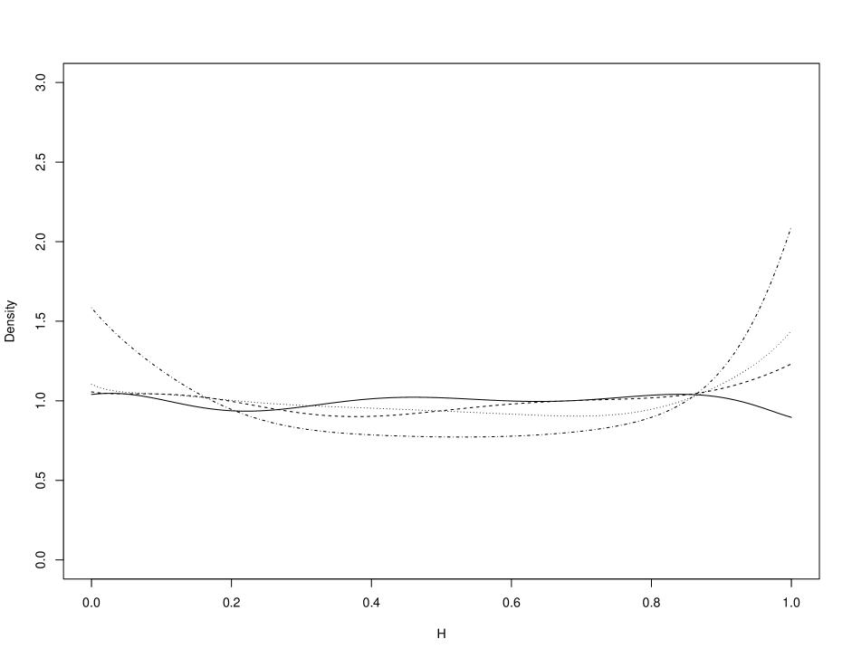
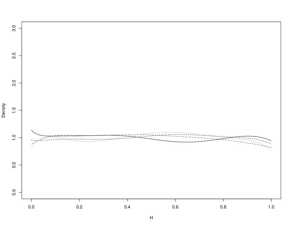
Figure 1: Density plots of $H$ with $n=100$ (left) and $n=10000$ (right). The solid, dashed, dotted and dotted dash lines represent results from $\alpha=0,1,10,100$ respectively.

3.2 Calibrating the scaling parameter in the Gibbs posterior

In the Gibbs posterior approach, the scaling parameter $\eta$ has to be specified before performing inference. There are several proposals based on different criteria, such as expected predictive loss (Grünwald and Van Ommen, 2017) and the posterior coverage rate (Syring and Martin, 2019). Data-driven approaches for estimating $\eta$ have been studied extensively, as the issue of mis-specification cannot guarantee that the posterior variance matches the sandwich variance obtained as in frequentist inference (Chernozhukov and Hong, 2003). Syring and Martin (2019) introduced a way to find the desired scaling using the frequentist bootstrap. At each bootstrap sample, if the coverage is not at the nominal level, then an adjustment is made to $\eta$ until the coverage meets the nominal level. The algorithm is described in Algorithm 4.

Data: $z_{1:n}=(z_{1},\ldots,z_{n})$

Given an tolerance $\epsilon<\kappa$ and $CR=1$, with an initial guess $\eta_{0}$ and $i=1$.

while $\left|CR-(1-\kappa)\right|>\epsilon$ do

      

      for $b=1,\ldots,B$ do

            

• Generate a bootstrap sample from the original sample, $z_{1:n}^{b}$.

• Get an empirical estimate for the parameter of interest, $\theta^{b}$ based on $z_{1:n}^{b}$.

• Obtain the posterior sample from $\pi(\theta|z_{1:n}^{b})$ based on $\eta_{i-1}$.

      Calculate the bootstrap mean $\bar{\theta}=B^{-1}\sum_{b=1}^{B}\theta^{b}$, and obtain the empirical coverage rate for $\bar{\theta}$,

$$CR=\frac{1}{B}\sum_{b=1}^{B}\mathbbm{1}(c^{b}_{\kappa/2}<\bar{\theta}<c^{b}_{1-\kappa/2})$$

where $\theta<c^{b}_{\kappa}$ satisfies $\kappa=\pi(\theta<c^{b}_{\kappa}|z_{1:n}^{b})$.

       Update $\eta$ as

$$\eta_{i}=\eta_{i-1}+i^{-0.51}\left[CR-(1-\kappa)\right],$$

and $i=i+1$.

return $\left(\eta_{1},\eta_{2},\ldots,\eta_{i}\right)$.

[6pt]

Algorithm 4 Algorithm to learn the Gibbs posterior scaling parameter $\eta$ (Syring and Martin, 2019).

In Sections 2.2 and 2.3, we generalized the previous Bayesian bootstrap approach, specifying a Dirichlet process posterior and predictive distribution, without requiring any scaling. Using this predictive approach, we propose a computationally-efficient way to calibrate $\eta$ so that the Gibbs posterior achieves nominal coverage.

The approach in Algorithm 4 is computationally intensive and MCMC is required for each bootstrap sample. Obtaining a posterior sample from Algorithms 1 and 2 is computationally less expensive, yet yields the correct marginal nominal coverage rate. Therefore we can utilize this posterior sample from predictive inference to adjust the posterior variance from the Gibbs posterior to achieve the valid uncertainty quantification. Furthermore, the approach of Syring and Martin (2019) is based on coverage adequacy. The method of Monahan and Boos (1992) is similarly used to assess coverage validity, and offers an alternative method for calibrating the Gibbs posterior by adjusting scaling parameter $\eta$ until the uniformity of the $H$ statistic is adequate. The process may be implemented efficiently using resampling ideas: a posterior sample obtained for $\eta=1$ (say), may be converted to an approximate sample for any other $\eta$ value for example by sampling-importance resampling.

As demonstrated in Chernozhukov and Hong (2003), under certain regularity conditions, the Gibbs posterior will be asymptotically normal with covariance matrix $\eta^{-1}(n\mathcal{J})^{-1}$ where $\mathcal{J}=-\mathbb{E}[\dot{\mathbf{U}}(\theta^{\ast})]$, $\mathbf{U}\left(\theta\right)={\partial\ell\left(z,\theta\right)}\big{/}{\partial\theta}$ and $\dot{\mathbf{U}}(\theta)={\partial\mathbf{U}(\theta)}\big{/}{\partial\theta^{\top}}$. Therefore, asymptotically, the Gibbs posterior concentrates on a $\sqrt{n}$-ball centered at $\theta^{\ast}$ with covariance matrix $\eta^{-1}(n\mathcal{J})^{-1}$. In order to have the similar coverage rate as predictive inference, we first obtain the sample posterior variance $V$ from the sample generated by Algorithm 1 or 2, then find the proportional rate $c$ so that $cV\approx(n\mathcal{J})^{-1}$, and therefore $\eta\approx c$ to achieve the similar uncertainty quantification. In practice, we do not know $(n\mathcal{J})^{-1}$ but can assess this value empirically. Algorithm 5 describes this algorithm in detail.

Data: $z_{1:n}=(z_{1},\ldots,z_{n})$

• Implement Algorithm 2 to obtain the posterior sample $(\theta^{1},\ldots,\theta^{S})$.

• Calculate the empirical posterior variance (or variance-covariance matrix) $V$.

• Obtain the posterior sample from $\pi(\theta|z_{1:n})$ and calculate the posterior variance (or variance-covariance matrix) $\widehat{\Sigma}$ based on an initial guess $\eta_{0}$.

• Modify $\eta$ based on $\widehat{\eta}V\approx\eta_{0}\widehat{\Sigma}$.

return $\widehat{\eta}$.

[6pt]

Algorithm 5 Algorithm to learn the Gibbs posterior scaling parameter $\eta$ by Bayesian predictive inference.

3.3 Calibration examples

To verify the performance of Algorithm 5, we implemented two examples from Syring and Martin (2019) that study problems concerning quantile regression and linear regression. In the quantile regression example, $\theta=(\theta_{0},\theta_{1})=(2,1)$ is the coefficient, and the data are generated from $Y\sim\mathcal{N}(\theta_{0}+\theta_{1}X,1)$ and $X+2\sim\chi^{2}(4)$. The loss function is specified as the mis-specified asymmetric Laplace likelihood, i.e.,

$$\ell_{n}((y_{i},x_{i})_{i=1}^{n},\theta)=\frac{1}{n}\sum_{i=1}^{n}\left|(y_{i}-x_{i}^{\top}\theta)(0.5-\mathbbm{1}_{(-\infty,x_{i}^{\top}\theta)}(y_{i}))\right|.$$

In the linear regression example, $\beta=(\beta_{0},\beta_{1},\beta_{2},\beta_{3})=(0,1,2,-1)$ represents coefficients in a linear predictor. We use the square loss in this case.

Table 2 shows the results from the two examples. All algorithms generate similar results in terms of the coverage probability and length in quantile regression, as there are only two parameters. All of the marginal coverage rates are close to the nominal level. The coverage rate of parameters are corrected to the nominal level if the coverage rate is slightly off in Algorithm 2. In the linear regression case, as there are four parameters, the marginal coverage probability is above the nominal level in Algorithm 4, as the algorithm is designed to primarily focus on the credible set. Algorithms 2 and 5 have similar results, and all marginal coverage probabilities are close to the nominal level. Even though Algorithm 5 has much lower computational burden, it still provides valid marginal uncertainty quantification. Therefore, we will use Algorithm 5 to calibrate the scaling parameter in the later examples.

Table 2: Comparison of 95% posterior credible intervals from Algorithm 2, and Gibbs posterior calibrating from Algorithms 4 and 5, based on 500 simulated datasets with $n=200$.

Coverage probability $\times$ 100 Average length $\times$ 100 Algorithm 2 Algorithm 4 Algorithm 5 Algorithm 2 Algorithm 4 Algorithm 5 Quantile regression example in Section 4 from Syring and Martin (2019) $\theta_{0}$ 96.8 96.4 96.2 70.6 71.4 70.1 $\theta_{1}$ 96.4 97.4 96.0 36.4 36.8 36.0 Linear regression example in the Supplementary material from Syring and Martin (2019) $\beta_{0}$ 94.6 99.0 97.8 46.1 78.2 54.2 $\beta_{1}$ 93.8 98.0 93.4 64.1 93.6 62.5 $\beta_{2}$ 93.6 99.2 93.6 63.9 100.3 62.4 $\beta_{3}$ 93.0 97.4 91.2 58.0 82.8 54.1

4 Asymptotic results

In this section, we establish the large sample properties of the proposed loss-type predictive-to-posterior calculation, under possible model mis-specification. The required assumptions (which relate to identifiability, and regularity of the loss function) are classical, and proofs are included in the Supplement. First, to show the consistency, we need to consider the limiting case as $n\longrightarrow\infty$. This requires $\widehat{\theta}$ in (1) to be degenerate at $\theta^{\ast}$ if all the information is available.

Theorem 1.

Suppose the prior $\pi_{0}(\theta)$ has full Hellinger support, and $\ell\left(z,\theta\right)$ is continuous $\forall\theta\in\Theta$ with

$$\int\log\left[1+\left|\ell\left(z,\theta\right)\right|\right]dG_{0}\left(z\right)<\infty.$$

Let $\theta^{s}_{1}=\theta(\varpi^{s})$ be the unique solution to

$$\min\limits_{\theta\in\Theta}\sum_{k=1}^{\infty}\varpi^{s}_{k}\ell\left(\zeta^{s}_{k},\theta\right)$$

for any given $\varpi^{s}$ and $\zeta^{s}$ generated from Algorithm 1. Let $\theta^{s}_{2}=\theta^{s}(z^{s})$ be the unique solution to

$$\min\limits_{\theta\in\Theta}\sum_{i=1}^{N}\ell\left(z^{s}_{i},\theta\right)$$

for integer $N$, and any given $z^{s}$ generated from Algorithm 2. Then

$$\sum_{k=1}^{\infty}\varpi^{s}_{k}\ell(\zeta^{s}_{k},\theta^{s}_{1})\longrightarrow\min\limits_{\theta\in\Theta}\int\ell\left(z,\theta\right)dF^{\ast}\left(z\right),\;\;\;\;\;\sum_{i=1}^{N}\ell(z^{s}_{i},\theta^{s}_{2})\longrightarrow\min\limits_{\theta\in\Theta}\int\ell\left(z,\theta\right)dF^{\ast}\left(z\right)$$

and $\theta_{1}^{s}\longrightarrow\theta^{\ast}$, $\theta_{2}^{s}\longrightarrow\theta^{\ast}$ almost surely as $n,N\longrightarrow\infty$.

We can also consider the limiting behavior of the estimator in terms of the probability law, specifically, that it exhibits posterior asymptotic normality. In the empirical measure, the estimating equation becomes $\sum_{i=1}^{n}\mathbf{U}_{i}(\theta)=\mathbf{0}$ and with some regularity conditions, we have that the frequentist solution $\widehat{\theta}_{n}$ has the property that

$$\sqrt{n}(\widehat{\theta}_{n}-\theta^{\ast})\xrightarrow{d}Normal_{p}(\mathbf{0},\mathbf{V})$$

where $\mathbf{V}=\mathcal{J}(\theta^{\ast})^{-1}\mathcal{I}(\theta^{\ast})\mathcal{J}(\theta^{\ast})^{-\top}$ with $\mathcal{I}(\theta^{\ast})=\mathbb{E}[\mathbf{U}(\theta^{\ast})\mathbf{U}(\theta^{\ast})^{\top}]$ and $\mathcal{J}(\theta^{\ast})=-\mathbb{E}[\dot{\mathbf{U}}(\theta^{\ast})$, both $(p\times p)$ matrices, and $\dot{\mathbf{U}}(\theta^{\ast})={\partial\mathbf{U}(\theta)}\big{/}{\partial\theta^{\top}}\big{|}_{\theta=\theta^{\ast}}$. The Bayesian analogy is the Bernstein-von Mises theorem, which establishes the limiting behaviour of the posterior distribution. We state the result in terms of the standardized parameter $\vartheta_{n,N}^{s}=\sqrt{N}(\theta^{s}-\widehat{\theta}_{n})$, where $\theta^{s}$ is a draw from Algorithm 1 or 2, and $\widehat{\theta}_{n}$ is the frequentist estimator.

Theorem 2.

Under Assumptions 1-6 in the Supplement, the probability that the posterior for $\vartheta_{n,N}^{s}$ assigns to an arbitrary set $A\subseteq\Xi$ converges to the mass given by a Normal measure. Specifically, if $\mathbf{Z}\sim Normal_{p}(\mathbf{0},\mathbf{V})$ is an arbitrary random variable independent from all other random variables, then $\pi(\vartheta_{n,N}^{s}\in A\left|z_{1:n}\right.)\to P(\mathbf{Z}\in A)$ as $n,N\to\infty$.

5 Doubly robust causal inference via propensity score regression

We now focus on the motivating example, which is a Bayesian representation for the DR regression approach to causal estimation. In a causal inference setting, for the $i$th unit of observation, $Y_{i}$ denotes a response, $d_{i}$ the treatment (or exposure) received, and $x_{i}$ a vector of pre-treatment covariates or confounder variables. Suppose the data generating structural model is

$$Y_{i}=\psi^{\ast}d_{i}+h_{0}(x_{i})+\epsilon_{i},\;\;\forall i=1,2,\ldots,n$$ (14)

where $\mathbb{E}\left[\epsilon_{i}\left|x_{i},d_{i}\right.\right]=0$ and $\text{Var}\left[\epsilon_{i}\left|x_{i},d_{i}\right.\right]=\sigma^{2}<\infty$, with $\epsilon_{1},\ldots,\epsilon_{n}$ independent, and where $h_{0}(x_{i})$ is an unknown real-valued function of the vector $x_{i}$. In this setting, $\psi^{\ast}$ is the ATE.

5.1 Frequentist inference in propensity score regression

A typical approach to causal adjustment uses the PS. With the PS estimated either via maximum likelihood or a fully Bayesian procedure summarized by the posterior mean, the outcome is modelled by adding the estimated PS (Robins et al., 1992), denoted $e\left(x_{i};\widehat{\gamma}\right)=\mathbb{P}\left(D_{i}=1\left|x_{i};\widehat{\gamma}\right.\right)$, where $\gamma$ is estimated via some form of binary regression, or via more flexible prediction approaches. Assume we specify the augmented model as

$$Y_{i}=\psi d_{i}+h_{1}(x_{i})+\phi e\left(x_{i};\widehat{\gamma}\right)+\epsilon_{i},\;\;\forall i=1,2,\ldots,n$$ (15)

and fit the model using ordinary least squares. The model in (15) leads to doubly robust inference. If $h_{1}(x)=h_{0}(x)$, so that (15) matches (14) and the model is correctly specified, then the estimator of the true ATE will be consistent irrespective of whether the PS model is correctly specified because the estimator $\widehat{\phi}$ will converge to zero as $n\longrightarrow\infty$; on the other hand, if the PS is correctly modelled, conditioning on it will block the confounding path from $D$ to $Y$ via $X$ so that $X\perp\!\!\!\perp D\left|\;e(X)\right.$, and (15) will still yield a consistent estimator of $\theta^{\ast}$, even if $h_{1}(x)$ is incorrectly specified. We will proceed by assuming that the functional forms of $h_{0}(x_{i},\beta_{0})$ and $h_{1}(x_{i},\beta)$ are parametric with associated parameter vectors $\beta_{0}$ and $\beta$. For example, linear regression assumes that $h_{0}(x_{i},\beta_{0})=x_{i}^{\top}\beta_{0}$ and $h_{1}(x_{i},\beta)=x_{i}^{\top}\beta$.

Let $z_{i}=(y_{i},d_{i},x_{i}),i=1,\ldots,n$, be the observed data, and $Z_{i}=(Y_{i},d_{i},x_{i}),i=1,\ldots,n$ be the random variable representing the random component in the conditional model. Estimation of $\theta=\left(\psi,\beta,\phi\right)$ in the conditional mean model (15) can proceed by defining a loss function which is the sum of squares of the residual error, i.e.,

$$\ell\left(z_{1:n},\theta\right)=\sum_{i=1}^{n}\left[y_{i}-\left(\psi d_{i}+h_{1}(x_{i},\beta)+\phi e\left(x_{i};\widehat{\gamma}\right)\right)\right]^{2}.$$ (16)

The method does not make any distributional assumption about $\epsilon_{i}$, and yields the solution

$$\widehat{\psi}=\frac{\sum\limits_{i=1}^{n}\left(d_{i}-e\left(x_{i};\widehat{\gamma}\right)\right)(y_{i}-h_{1}(x_{i},\widehat{\beta})-\phi e\left(x_{i};\widehat{\gamma}\right))}{\sum\limits_{i=1}^{n}\left(d_{i}-e\left(x_{i};\widehat{\gamma}\right)\right)d_{i}}.$$

This is the feasible G-estimator, proposed in Robins et al. (1992), which is consistent for $\psi^{\ast}$ and robust to mis-specification. A key aspect of this frequentist approach is the use of plug-in estimation for parameter $\gamma$; it can be demonstrated that this approach provides locally efficient estimation of $\psi$ under the assumption that the PS model is correctly specified at least up to a finite dimensional parameter that may itself be estimated consistently at the usual parametric rate. Non-parametric estimation of the propensity model can also preserve consistent and efficient estimation of $\psi$, provided the rate of convergence of the non-parametric estimator is fast enough, and this can be achieved by using many standard flexible or machine learning approaches.

5.2 Bayesian inference in propensity score regression

The plug-in approach can also be justified in a fully Bayesian framework under the loss-based formulation. McCandless et al. (2010) and Jacob et al. (2017) demonstrate how to block the flow of the information from the PS to the outcome regression when implementing MCMC in a joint model of the treatment and outcome. However, this approach induces finite sample bias and is not ideal for small sample inference. A two-step approach, which assumes a complete separation in inference between the PS and outcome models and uses a plug-in estimate of $\gamma$ in (15) also yields a valid Bayesian solution; see Stephens et al. (2022) for further discussion. This approach has been shown to provide superior estimation, and we adopt it in the following analysis. The loss function used in (5) or (8) should incorporate components for parameters in both the outcome model and the PS model, say

$$\ell(z,(\theta,\gamma))=\ell_{1}(z,(\theta,\widehat{\gamma}))+\ell_{2}(z,\gamma)$$

where $\widehat{\gamma}$ is the minimizer of $\ell_{2}(\ldotp,\gamma)$ alone, with optimization over both sets of parameters carried out for each sampled realization from the non-parametric posterior distribution.

We deploy the Dirichlet process formulation from Section 2.3. In the outcome regression setting, we assume that the predictive resampling is implemented through residuals arising from the outcome model (Wade, 2013; Quintana et al., 2020). In this case, we first draw each pair of $\left\{{x}^{s}_{i},d^{s}_{i}\right\}$, $i=1\ldots,N$, from the empirical distribution as the DP with $\alpha=0$, and then obtain the fitted values $e\left({x}^{s}_{i},\widehat{\gamma}^{s}\right)$ from a propensity score model based on logistic regression, refitted to the newly sampled $\left\{{x}^{s}_{i},d^{s}_{i}\right\}$ data set. Then we simulate $y_{i}^{s}$ from a DP model with the conditional base measure $G_{0}\equiv\mathcal{N}\left(\psi d^{s}_{i}+h_{1}\left({x}^{s}_{i},\beta\right)+\phi e\left({x}^{s}_{i},\widehat{\gamma}^{s}\right),1\right)$, where $\theta=\left(\psi,\beta,\phi\right)$ is generated from its prior distribution.

Corollary 1.

The posterior distribution for the causal parameter, $\psi$ in (15), becomes degenerate at $\psi^{\ast}$ as $n\longrightarrow\infty$ if either the outcome model or PS model is correctly specified. In addition, a posteriori, $\theta\xrightarrow{d}\mathcal{N}\left(\theta^{\ast},V_{\theta^{\ast}}\right)$ where $V_{\theta^{\ast}}=\mathcal{J}(\theta^{\ast})^{-1}\mathcal{I}(\theta^{\ast})\mathcal{J}(\theta^{\ast})^{-\top}$.

Proof.

When we have a mis-specified PS model and a correctly specified OR model, $\theta^{\ast}=\left(\psi^{\ast},\beta^{\ast},0\right)$. The results follow by applying Theorem 2. When the outcome model is mis-specified but the PS model is correctly specified, $X\perp\!\!\!\perp D\left|e\left(x;\gamma^{\ast}\right)\right.$ and $\widehat{\gamma}\longrightarrow\gamma^{\ast}$. Therefore, $e\left(x;\widehat{\gamma}\right)$ is an asymptotic balancing score. Suppose we specify the mean model as above and assume that the effect of $D$ is captured via the term $\psi D$. Under the assumption of no unmeasured confounding, we can find $\theta^{\ast}=\left(\psi^{\ast},\beta^{\ast},\phi^{\ast}\right)$ under the specified loss function corresponding to such mis-specified OR models. This is again in line with the standard frequentist approach for mis-specified models. Therefore, we can construct the same asymptotic results as for the mis-specified PS case by applying Theorem 2. ∎

6 Simulation studies

We examine the performance of the Bayesian methods described in Section 2 with the two updating frameworks. For each example, we consider

• Method I: Gibbs posterior computed using MCMC, calibrating $\eta$ via Algorithm 5;

• Method II: Prior-to-posterior inference via the Bayesian bootstrap from (5);

• Method III: Predictive-to-posterior inference via Algorithm 2.

6.1 Example 1

In this example, we consider the simulation study constructed by Saarela et al. (2016). The data are simulated as follows: we simulate $X_{1},X_{2},X_{3},X_{4}\sim\mathcal{N}\left(0,1\right)$ independently, and then set

$$U_{1} =\frac{\left|X_{1}\right|}{\sqrt{1-2/\pi}}$$

$$D\left|U_{1},X_{2},X_{3}\right. \sim\text{ Bernoulli}\left(\text{expit}\left(0.4U_{1}+0.4X_{2}+0.8X_{3}\right)\right)$$

$$Y\left|D,U_{1},X_{2},X_{4}\right. \sim\mathcal{N}\left(D-U_{1}-X_{2}-X_{4},1\right)$$

Three scenarios are considered:

• Scenario A: Mis-specify the OR model using covariates $(x_{1},x_{2},x_{4})$ and correctly specify a treatment assignment model using covariates $(u_{1},x_{2},x_{3})$.

• Scenario B: Correctly specify the OR model using covariates $(u_{1},x_{2},x_{4})$ and mis-specify a treatment assignment model using covariates $(x_{1},x_{2},x_{3})$.

• Scenario C: Mis-specify the OR model using covariates $(x_{1},x_{2},x_{4})$ and mis-specify a treatment assignment model using covariates $(x_{1},x_{2},x_{3})$. This is not originally considered in Saarela et al. (2016).

The prior-to-posterior update via the Gibbs posterior is implemented using MCMC and the Bayesian bootstrap approaches from Sections 2.4 and 2.2, and non-informative priors are placed for all the parameters with $10,000$ MCMC samples and $1,000$ burn-in iterations. For the predictive-to-posterior update, we generate $S=1,000$ sets, each with $N=10,000$ new data points and with $\alpha=1$. For $n=20$, we also place an informative normal prior with mean at the true value and standard deviation 2 for the Gibbs posterior using MCMC.

The results are given in the Supplement, and the table shows the results of $1,000$ Monte Carlo replicates of the averages of the posterior means, variances and coverage rates for $\theta$ with different sample sizes. Coverage rates are computed by constructing a 95% credible interval for $\theta$ from the 2.5% and 97.5% posterior sample quantiles. When the sample size is small, the Bayesian bootstrap (Method II) and predictive inference models (Method III) exhibit poor coverage while the Gibbs posterior (Method I) returns coverage rates at the nominal level; however, Method II presents rather larger variances. The results for the Gibbs posteriors with $\eta=1$ display the correct posterior mean, but the coverage is significantly below the nominal level in Scenarios A and B, which confirms that the calibration of $\eta$ is required. The difference in variances diminishes as the sample size increases, or when the informative prior is considered (demonstrated in the bracket for $n=20$). As expected, the two updating approaches yield unbiased estimates in both scenarios and show agreements in the variance and the coverage rate when the sample size is over 100. The Bayesian bootstrap and DP-based predictive inference generate similar results, as the prior does not carry much weight when $\alpha/N$ is small. When both models are mis-specified, all cases yield significantly biased estimates unless the informative prior is used.

6.2 Example 2: High-dimensional case

In this example, we examine the performance of the proposed updating approaches under high denominational settings, with binary exposure. The data are simulated as follows: we simulate $X=(X_{1},X_{2},\ldots,X_{p})\sim\mathcal{N}_{p}\left(0,\Sigma\right)$ and $\Sigma_{ij}=1$ if $i=j$ and 0.1 otherwise, and then simulate

$$D\left|X\right. \sim\text{ Bernoulli}\left(\text{expit}\left(0.3X_{1}+0.2X_{2}-0.4X_{5}+1.3X_{2}X_{5}+1.8X_{1}X_{2}\right)\right)$$

$$Y\left|D,X\right. \sim\mathcal{N}\left(D+0.5X_{1}+X_{3}-0.1X_{4}-0.2X_{7}+1.5X_{3}X_{4}+0.6X_{7}^{2}+1.2X_{1}X_{3},1\right).$$

In the analyses, we take $p=20$ and $n=50$ and $100$.

The loss function adopted for the loss-based analysis for Method II and Method III encompasses both the need to penalize the number of terms in the PS model and the need to select a penalization parameter. We use penalized logistic regression for the PS model including all $x_{1},\ldots,x_{p}$ and first order interactions between them, giving a total of $q=p+p(p-1)/2$ parameters. Specifically, we use the lasso penalty, and base conclusions on the loss function

$$\ell_{2}((x,d),(\gamma,\lambda))=-\log f_{D|X}(d|x,\gamma)+\lambda\sum_{j=1}^{q}\left|\gamma_{j}\right|$$

where $f_{D|X}(d|x,\gamma)$ is the Bernoulli mass function with logistic link. This loss function is then incorporated into a cross-validation procedure to define the loss to be deployed in the implementation of Methods II and III, $\ell_{\text{CV}}((x,d),(\gamma,\lambda))$ say, which takes the input data and returns optimized values of $\gamma$ and $\lambda$, as well as the fitted values that can be transported into the outcome model. The value of $\lambda$ is estimated with lowest test mean squared error over 10-fold cross validation. For the outcome model, we fit the model with the treatment indicator and estimated PSs only as covariates. For Method II, we set $S=1000$. For the predictive-to-posterior update, we generate $S=1000$ sets, each with $N=100$ and $\alpha=5$. For comparison, we also consider the Bayesian doubly robust high-dimension (BDR-HD) method proposed in Antonelli et al. (2022), where the PS and outcome are estimated via regression models with the Gaussian process (GP) prior, and then the MCMC estimate is plugged in to a doubly robust estimator. The variance is adjusted through the frequentist bootstrap so that it will achieve frequentist nominal coverage rate. For the BDR-HD method, we ran 500 iterations with 100 burn-in iterations for both the PS and OR models.

Table 3: Example 2: Simulation results of the marginal causal contrast under high-dimensional settings, with true value equal to 1, on 500 simulation runs on generated datasets of size $n$. BDR-HD represents the method proposed in Antonelli et al. (2022), and Running time represents the average running time per Monte Carlo replicate in minutes.

$n$ Method 50 100 Bias Method II 0.081 0.022 Method III 0.216 0.260 BDR-HD 0.232 0.112 RMSE Method II 0.854 0.574 Method III 0.761 0.566 BDR-HD 0.728 0.343 Coverage rate Method II 99.4 98.6 Method III 94.0 96.4 BDR-HD 98.0 97.8 Running time Method II 1.73 2.33 Method III 1.81 1.99 BDR-HD 15.19 32.36

The results are given in Table 3. Method II shows the smallest bias among all methods, while Method III both exhibit some biases in $n=50$ and $n=100$; this is primarily due to the bias from the fitted PS via the lasso penalty. Additionally, the outcome model specified in Methods II and III only contains the PS and an intercept to account for confounding. However, the coverage rate is still around the nominal level for both methods. If the PS is more accurately estimated, the bias would diminish and the coverage rate would achieve the target level as suggested by the additional simulation study in the Supplement. Method III shows a larger bias due to the impact of the new data which are generated from a mis-specified model. The BDR-HD method exhibits small biases in both cases, and the coverage rates are around nominal level. In this method, it utilizes component-wise GP regression for each confounder in treatment and outcome models, and interaction terms are supplied in the GP regression as separate covariates. Therefore, it achieves desired performance. However, in practice, this might not be feasible as it will include $p(p-1)/2$ additional covariates, increasing the computational complexity by at least $O(p^{2})$. It also should be noted that BDR-HD has a much higher the computational burden than Method II and Method III as it requires much longer time on average per replicate, as it includes MCMC computation for GP regression and an additional bootstrap step to adjust the posterior variance.

6.3 Example 3: Comparison with flexible modelling approaches

In this example, we seek to compare the proposed approach with existing flexible/machine learning causal estimation approaches. We compare Method III with Bayesian causal forests (BCFs, Hahn et al. (2020)), and double machine learning (DML) (Chernozhukov et al., 2018) using a variety of machine learning strategies. The Supplement provides the details of the data generation settings, and a description of those approaches. Table 4 displays the results of this study. The BCFs display certain bias in the small size, but has a relatively small variance, and therefore lower RMSE than Method III. All DML results show quite significant biases, and they do not vanish as the sample size increases. However, the variances are smaller than other approaches, and therefore the RMSEs are similar to the other two methods. As for the coverage rate, the coverage of DML is decreasing dramatically as $n$ increases and ultimately is below the target level, except the regression tree and random forest, which shows over-coverage in those cases. The BCF is consistenly below the nominal level, while Method III yields a coverage rate at the nominal level in all cases. Note, however, that the BCF and DML methods do not assume a known functional form for the treatment effect model, which is needed for PS regression. Note also that the BCF and DML methods require significantly more computational time than Method III.

Table 4: Comparison of results for the proposed Bayesian empirical likelihood, Bayesian causal forests (BCFs) and frequentist double machine learning estimator (DML). Summary of $1,000$ simulation runs. Rows correspond to the bias, root mean square error (RMSE), and coverage rates.

$n$ Method 500 1000 2000 Bias Method III 0.076 0.037 0.005 BCF 0.157 0.111 0.073 DML-Tree -0.348 0.023 0.122 DML-Forest 0.252 0.087 0.126 DML-Boosting -0.147 0.219 0.231 DML-Nnet -0.090 0.215 0.212 DML-Ensemble -0.022 0.217 0.233 DML-Best -0.111 0.211 0.212 RMSE Method III 0.561 0.395 0.270 BCF 0.289 0.195 0.130 DML-Tree 0.256 0.180 0.180 DML-Forest 0.245 0.187 0.168 DML-Boosting 0.276 0.265 0.254 DML-Nnet 0.339 0.268 0.237 DML-Ensemble 0.262 0.263 0.255 DML-Best 0.302 0.263 0.236 Coverage rate Method III 92.9 93.9 95.2 BCF 84.9 83.6 84.3 DML-Tree 99.7 99.7 97.2 DML-Forest 99.1 98.3 92.2 DML-Boosting 92.4 76.9 49.3 DML-Nnet 91.3 75.6 53.7 DML-Ensemble 94.0 77.4 49.4 DML-Best 89.6 76.1 53.4

7 Application: UK Speed Camera Data

Our real example aims to quantify the causal effect of speed camera presence on road traffic collision. We use data on the location of fixed speed cameras for 771 camera sites in the eight English administrative districts, including Cheshire, Dorset, Greater Manchester, Lancashire, Leicester, Merseyside, Sussex and the West Midlands. These data form the ‘treated’ group. For the ‘untreated’ group, we randomly select a sample of 4,787 points on the network within our eight administrative districts. Details of these data can be found in Graham et al. (2019).

The outcome of interest is the number of personal injury collisions per kilometre. The data are taken from police reports collated and processed by the Department for Transport in the UK in the ‘STATS 19’ data set. The location of each personal injury collision is recorded using the British National Grid coordinate system and can be located on a map using Geographical Information System software. Data are collected from 1999 to 2007 to ensure the availability of collision data for the years before and after the camera installation for every camera site as speed cameras were introduced varying from 2002 to 2004. There is a formal set of location selection guidelines for speed cameras in the UK (Gains et al., 2004). These guidelines inform the selection of covariates which represent the characteristics of units that simultaneously determine the treatment assignment (camera location) and outcome (number of accidents). Primary guidelines for site section include the site length, the number of fatal and serious collisions and the number of personal injury collisions in a preceding time period. In addition, drivers might try to avoid the routes with speed cameras, and the reduction in collisions may come from a reduced traffic flow. Therefore, we include the annual average daily flow (AADF) as a confounder to control the effect due to the traffic flow. We also include factors that would have additional safety impacts, such as road types, speed limit, and the number of minor junctions within site length (Christie et al., 2003).

We apply the proposed Bayesian methods to the speed camera data with the loss defined in (16). Graham et al. (2019) estimated the PS with a generalized additive model by including smooth functions on the AADF and the number of minor junctions and achieved balance and overlap. For the outcome model, we include all the confounders and the estimated PS. We place non-informative priors for all the parameters in prior and predictive inference based on the general DP representation with $\alpha=100$ and $N=10,000$. Table 5 shows summary statistics of the ATE based on $20,000$ posterior samples. All methods indicate that the installation of a speed camera can reduce road traffic collisions, by approximately 1.4 incidents per site on average; however, we notice that the Bayesian bootstrap based approaches yield a slightly higher variation. The Gibbs posterior (Method I) has similar variance to the other two methods when calibrated using Algorithm 5 with $\eta=0.024$, which is close to the calibration achieved by the estimated residual variance ($0.027$). We report the posterior predictive distribution of the percentage reduction in an average change in road traffic collisions that is attributable to speed cameras Table 5 (Graham et al., 2019). PS regression demonstrates that there is about an 18% reduction in road traffic collisions in locations where a speed camera is installed, indicating a stronger causal relationship than that estimated by inverse probability weighting (IPW) computed using a Bayesian approach. All three loss-bases methods show similar posterior densities for the change in the ATE (Figure presented in the Supplement), while Method III shows a slightly smaller variance. Compared to the IPW analysis, which only relies on the inverse weighting adjustment, PS regression has an additional treatment-free component, and therefore offers an additional degree of robustness if one of the component models is correctly specified. We obtain narrower 95% credible intervals and smaller standard deviations because regression-based approaches, coupled with the Bayesian bootstrap strategy, reduces the influence of extreme PS values on ATE estimation.

Table 5: Summary statistics for the posterior distribution of the ATE, and the posterior predictive distribution of the percentage change of the ATE for speed camera data. IPW-BB represents results using the update two-step Bayesian bootstrap approach based on inverse probability weighting estimation, while IPW-BB (plug-in) represents the plug-in approach using the two-step Bayesian bootstrap.

	Posterior Mean	Standard Deviation	95% Credible Interval
ATE
Method I	-1.413	0.183	(-1.771, -1.054)
Method II	-1.411	0.184	(-1.772, -1.048)
Method III	-1.413	0.180	(-1.767, -1.058)
IPW-BB	-1.089	0.203	(-1.486, -0.679)
IPW-BB (plug-in)	-1.088	0.209	(-1.484, -0.663)
Percentage Change of the ATE
Method I	-18.656	2.356	(-23.250, -13.996)
Method II	-18.603	2.352	(-23.224, -13.951)
Method III	-18.659	2.313	(-23.194, -14.070)
IPW-BB	-14.338	2.622	(-19.419, -9.036)
IPW-BB (plug-in)	-14.625	2.807	(-19.978, -8.877)

8 Discussion

We have formulated inference for parameters defined via loss functions in a formal Bayesian approach that does not rely on standard prior-likelihood calculations. The usual prior updating framework provides a means of informed and coherent decision making in the presence of uncertainty. Predictive inference sheds light on how to quantify Bayesian uncertainty, where the model is specified via a sequence of predictive distributions without a prior-likelihood construction, and often yields a computationally more efficient calculation because it relies purely on optimization instead of integration via MCMC.

We focused on non-parametric approaches based on the Dirichlet process. First, from the traditional Bayesian updating approach, we obtained the posterior distribution from a loss-based decision-theoretic perspective. Secondly, by sequentially imputing sets of unobserved future data, we computed the posterior by minimizing a loss function over the future data. We also showed that computations following this paradigm yield valid posterior inference in the spirit of Monahan and Boos (1992). Using this method, we calibrated the scaling parameter of the Gibbs posterior, and demonstrated it yielded valid uncertainty quantification. We gave asymptotic results that showed the consistency and asymptotic normality of the computed posterior distributions. Simulation examples demonstrated that proposed approaches have good Bayesian and frequentist properties, and are typically less computationally burdensome that other successful Bayesian approaches.

Finally, we applied the loss-based approaches to study road safety outcomes, and quantified the causal effect of speed cameras on road traffic accidents, concluding that the presence of speed cameras can reduce the number of personal injury collisions. Such inference aids transportation authorities to propose a more effective targeted installation plan of speed cameras to improve road safety. Bayesian methods are generally applicable in causal inference for real applications, and yield interpretable variability estimates in finite samples.

The principles presented in this paper can also be applied in much more general settings, when likelihood functions are not available. In addition, the proposed methodology can be widely applied in other causal settings when the traditional Bayesian set-up requires over-specifying the model condition, clashing with the partial specified restriction.

Supplementary materials for “Assessing the validity of Bayesian inference using loss functions”

Appendix A Estimation via predictive inference and the KL divergence

The Bayes estimator of the a target parameter is the function of the data that minimizes the posterior expected loss, given by

$$\arg\min\limits_{t\in\Theta}\int_{\Xi}u\left(t,\xi\right)\pi\left(\xi|z_{1:n}\right)\ d\xi.$$

If $u$ is taken to be the KL divergence between the true model, $f^{\ast}$ and a possibly mis-specified model, $f$, given by

$$u\left(\theta,\xi\right)=\int\log\left(\dfrac{f^{\ast}(z|\xi)}{f(z|\theta)}\right)f^{\ast}(z|\xi)\ dz,$$

then the optimization becomes

$$\arg\min\limits_{t\in\Theta}\int_{\Xi}\left\{\int\log\left(\dfrac{f^{\ast}(z|\xi)}{f(z|t)}\right)f^{\ast}(z|\xi)\ dz\right\}\pi\left(\xi\left|z_{1:n}\right.\right)\ d\xi=\arg\max\limits_{t\in\Theta}\int\log f(z|t)p^{\ast}(z|z_{1:n})\ dz.$$ (17)

Exchanging differentiation and integration, we can deduce that the solution to (17) is also the solution to the estimating equation

$$\int\frac{\partial\log f(z|t)}{\partial t}p^{\ast}(z|z_{1:n})dz=\int S(z,t)p^{\ast}(z|z_{1:n})dz=0$$

where $S(z,\theta)$ is the score function. The minimization in (17) does not involve prior opinion concerning $\theta$, but (17) can be modified to

$$\arg\max\limits_{t\in\Theta}\left\{\int(\log f(z|t)+\log\pi_{0}(t))p^{\ast}(z|z_{1:n})\ dz\right\}$$

or via the modified score function

$$S^{*}(z,\theta)=S(z,\theta)+\frac{\partial}{\partial\theta}\log\pi_{0}\left(\theta\right).$$

A sample from $p^{\ast}(z|z_{1:n})$ can be converted to a sampled value of $\theta$ in the same fashion as discussed in the main paper, which yields a fully Bayesian procedure with the solution of the usual likelihood-based posterior distribution.

Appendix B Assessing validity of non-standard posterior inference

We investigate the validity of the proposed predictive inference approach under mis-specification. We simulate data based on the set up from Example 1 in Section 6 in the main paper, where the loss function is specified as a squared loss, and generate the values of coefficients in the outcome model from the prior distribution, that is, from the Normal distribution with mean the same as the example and variance 10,000, with the outcome data generated from the correct outcome regression model. This procedure is repeated $1,000$ times with $n=100$ and $n=10,000$. For each dataset, we perform the proposed predictive-to-posterior Bayesian inference method for various $\alpha$ values, where we produce the posterior distribution of the average treatment effect based on a mis-specified propensity score model and a mis-specified outcome model (with the treatment variable and the estimated propensity score). In this case, the computed posterior will not concentrate at the true value as $n$ grows.

In all cases, the posterior distribution computed using predictive-to-posterior inference fails the Monahan & Boos uniformity test, with $p$-values all smaller than $10^{-6}$. This is confirmed by the density plots in Figure 2, where they exhibit higher densities at the tails.

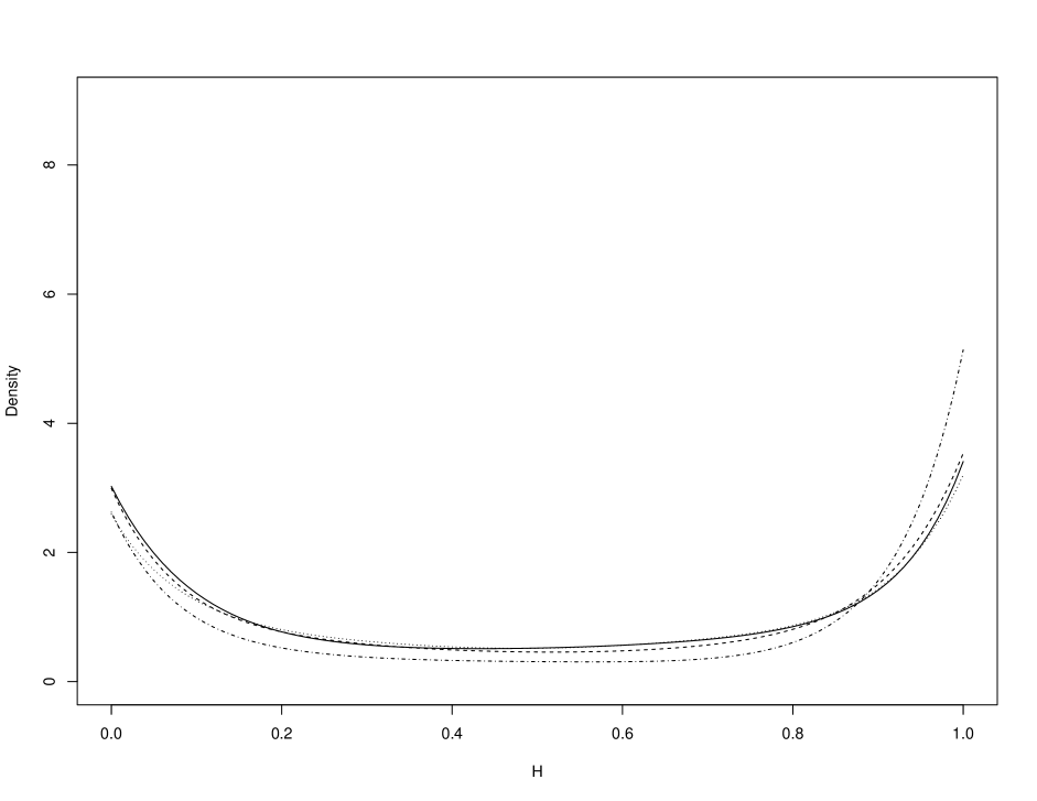
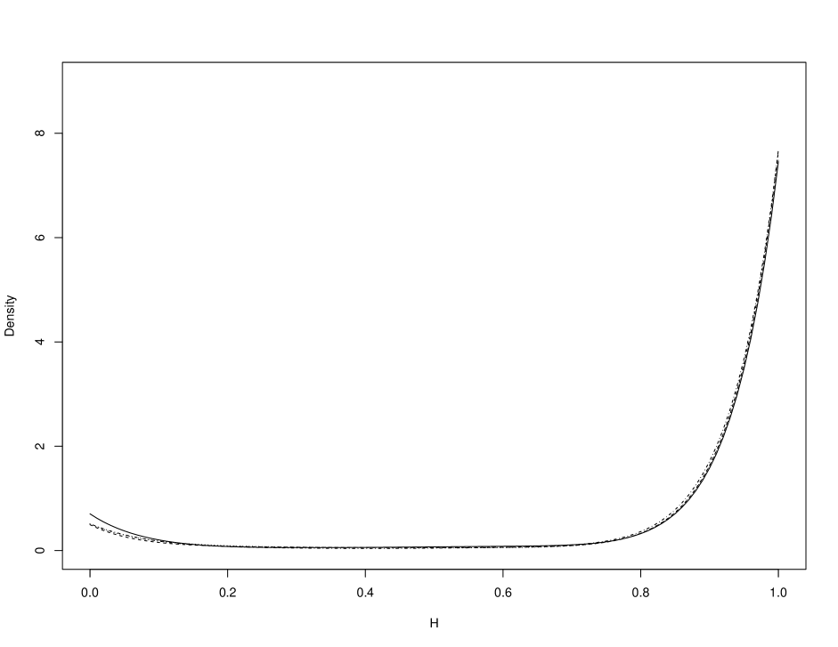
Figure 2: Checking coverage validity using Monahan & Boos: Density plots of $H$ with $n=100$ (left) and $n=10000$ (right) under a mis-specified model. The solid, dashed, dotted and dotted dash lines represent results from $\alpha=0,1,10,100$ respectively.

Appendix C Asymptotics

C.1 Definition of Bayesian Consistency

Definition 1.

(Walker and Hjort, 2001) For realizations $z_{1},z_{2},\ldots,z_{n}$ drawn independently from some unknown underlying distribution $F^{\ast}$ with true data generating value $\theta^{\ast}$ in the interior of the parameter space $\Theta$, the posterior mass assigned to $A\subseteq\Theta$ is given by

$$\Pi^{n}\left(A\right)=\pi\left(\theta\in A\left|z_{1},\ldots,z_{n}\right.\right)=\dfrac{\displaystyle\int_{A}R_{n}\left(\theta\right)\pi_{0}\left(d\theta\right)}{\displaystyle\int R_{n}\left(\theta\right)\pi_{0}\left(d\theta\right)}$$

where

$$R_{n}\left(\theta\right)=\prod_{i=1}^{n}\exp\left[-\left\{\ell\left(z_{i},\theta\right)-\ell\left(z_{i},\theta^{*}\right)\right\}\right]$$

and where $\pi_{0}\left(\theta\right)$ is the prior density for $\theta$. If $A_{\epsilon}=\left\{\theta:d(\theta,\theta^{*})>\epsilon\right\}$ where $d(\theta,\theta^{\ast})$ is some distance measure, the posterior distribution is consistent in the Bayesian sense if $\Pi^{n}\left(A_{\epsilon}\right)\longrightarrow 0$ almost surely under $F^{\ast}$.

C.2 Assumptions

Assumption 1.

The loss function $\ell(\theta,z):\Theta\times\mathbb{Z}\to\mathbb{R}$ is a measurable function, bounded from below, with

$$\int\ell\left(z,\theta\right)dF^{\ast}\left(z\right)<\infty\qquad\forall\theta\in\Theta$$

where $\Theta$ is a compact and convex subset of a $p$-dimensional Euclidean space.

Assumption 2.

$\ell\left(z,\theta\right)$ is continuous $\forall\theta\in\Theta$.

Let $\mathbf{U}_{i}\left(\theta\right)={\partial\ell\left(z_{i},\theta\right)}\big{/}{\partial\theta^{\top}}$. Minimizing the expected loss function, $\mathbb{E}_{F^{\ast}}[\ell\left(Z,\theta\right)]$, is equivalent to solving a $p\times 1$ system of estimating equations given by $\mathbb{E}_{F^{\ast}}[\mathbf{U}(\theta)]=\mathbf{0}$, with expectations taken with respect to the true data generating model $F^{\ast}$.

Assumption 3.

$\theta^{\ast}\in\Theta$ is the unique solution to $\mathbb{E}_{F^{\ast}}[\mathbf{U}(\theta)]=\mathbf{0}$, and for arbitrary $\delta>0$, there exists an $\epsilon>0$ so that

$$\lim\limits_{n\longrightarrow\infty}\mathbb{P}\left(\sup_{\left\lVert\theta-\theta^{\ast}\right\rVert\ >\ \delta}\frac{1}{n}\sum_{i=1}^{n}\left(\ell(z_{i},\theta)-\ell(z_{i},\theta^{\ast})\right)<\epsilon\right)=1.$$

Assumption 4.

$\mathbb{E}\left[\sup_{\theta\in\Theta}\left\lVert\mathbf{U}\left(\theta\right)\right\rVert^{\gamma}\right]<\infty$ for $\gamma>2$. Suppose there exists a neighborhood, $\widetilde{\Theta}$ of $\theta^{\ast}$ within which ${\mathbf{U}}(\theta)$ is continuously differentiable.

$$\mathbb{E}_{F^{\ast}}\left[\sup_{\theta\in\Theta^{*}}\left\lVert\dot{\mathbf{U}}(\theta)\right\rVert_{F}\right]<\infty,$$

with $\left\lVert\cdot\right\rVert_{F}$ denoting the Frobenius norm.

Assumption 5.

There is an open ball $B$ containing $\theta^{\ast}$ such that all first, second and third partial derivatives of $\ell(\theta,z)$ with respect to $\theta\in B$ exist and are continuous for all $z$. Furthermore, there exist measurable functions $G_{j}$, $G_{jk}$, $G_{jkl}$ and $M_{jkl}$ such that for $\theta\in B$ we have

$$\left|\frac{\partial\ell\left(z,\theta\right)}{\partial\theta_{j}}\right| \leq G_{j}(z) \text{with }\displaystyle\int G_{j}(z)dF^{\ast}\left(z\right)<\infty,$$

$$\left|\frac{\partial^{2}\ell\left(z,\theta\right)}{\partial\theta_{j}\partial\theta_{k}}\right| \leq G_{jk}(z) \text{with }\displaystyle\int G_{jk}(z)dF^{\ast}\left(z\right)<\infty,$$

$$\left|\frac{\partial^{3}\ell\left(z,\theta\right)}{\partial\theta_{j}\partial\theta_{k}\partial\theta_{l}}\right| \leq G_{jkl}(z) \text{with }\displaystyle\int G_{jkl}(z)dF^{\ast}\left(z\right)<\infty,$$

$$\left|\frac{\partial\ell\left(z,\theta\right)}{\partial\theta_{j}}\frac{\partial^{2}\ell\left(z,\theta\right)}{\partial\theta_{k}\partial\theta_{l}}\right| \leq M_{jkl}(z) \text{with }\displaystyle\int M_{jkl}(z)dF^{\ast}\left(z\right)<\infty.$$

Let

$$\mathcal{I}(\theta^{\ast})=\mathbb{E}[\mathbf{U}(\theta^{\ast})\mathbf{U}(\theta^{\ast})^{\top}]\qquad\qquad\mathcal{J}(\theta^{\ast})=-\mathbb{E}[\dot{\mathbf{U}}(\theta^{\ast})]$$

both $(p\times p)$ matrices, and $\dot{\mathbf{U}}(\theta^{\ast})={\partial\mathbf{U}(\theta)}\big{/}{\partial\theta^{\top}}\big{|}_{\theta=\theta^{\ast}}$

Assumption 6.

$\mathcal{I}(\theta)$ and $\mathcal{J}(\theta)$ are non-singular and $\mathcal{J}$ is full rank, rank$\left(\mathcal{J}(\theta)\right)=p$, for $\theta\in B$, with all elements finite.

C.3 Proof of Theorem 1

Proof.

Suppose that $\theta^{s}_{1}$ is the minimizer of the weighted loss

$$\theta^{s}_{1}\equiv\theta(\varpi^{s})=\arg\min_{t}\sum_{k=1}^{\infty}\varpi_{k}^{s}\ell\left(\zeta_{k}^{s},t\right).$$

given by the prior-to-posterior computation. From Theorem 1 in Lijoi et al. (2004), there exists an unique random element $F_{1}$ such that

$$\sum_{k=1}^{\infty}\varpi_{k}^{s}\ell(\zeta_{k}^{s},\theta^{s})\longrightarrow\min\limits_{t\in\Theta}\int\ell\left(z,t\right)dF_{1}\left(z\right)\;\;\;n\longrightarrow\infty.$$

It remains to show that $F_{1}\equiv F^{\ast}$. As $F_{1}$ is a draw from the posterior distribution under a Bayesian non- parametric formulation given by the prior-to-posterior computation, according to the de Finetti’s representation theorem, the posterior distribution will be degenerate at $F^{\ast}$ as $n\longrightarrow\infty$. Therefore, $\theta(\varpi^{s})$, is unique for any given $\zeta^{s}$ and $\varpi^{s}$, $\theta(\varpi^{s})$ will be become degenerate at $\theta^{\ast}$ as $n\longrightarrow\infty$.

Alternatively, suppose that $\theta^{s}_{2}$ is the minimizer of the Monte Carlo estimate of the posterior predictive expectation

$$\theta^{s}_{2}\equiv\theta\left(z^{s}\right)=\arg\min_{t}\sum_{i=1}^{N}\ell\left(z^{s}_{i},t\right).$$

Again by Theorem 1 in Lijoi et al. (2004), there exists an unique random element $F_{2}$ such that

$$\sum_{k=1}^{N}\ell(z_{k}^{s},\theta^{s}_{2})\longrightarrow\min\limits_{t\in\Theta}\int\ell\left(z,t\right)dF_{2}\left(z\right)\;\;\;n,N\longrightarrow\infty.$$

These results confirm that the posterior distribution generated by each approach converges weakly to a probability measure with all its mass on $F_{2}\equiv p(z^{s}_{1:N}|z_{1:n})$, and It also remains to show that $F_{2}\equiv F^{\ast}$. Under mild regularity conditions and the correct specification of the model leading to $\pi^{\ast}(\xi\mid z_{1:n})$, with $\widehat{\xi}\left(z_{1:n}\right)$ in a neighbourhood of $\xi^{\ast}$, following Bernardo (1979), we have

$$p^{\ast}(z^{s}_{1},\ldots,z^{s}_{N}|z_{1:n}) =p^{\ast}(z^{s}_{1},\ldots,z^{s}_{N}\mid\widehat{\xi}(z_{1:n}))+\textrm{O}(1)$$

$$=p^{\ast}(z^{s}_{N}\mid z^{s}_{1},\ldots,z^{s}_{N-1},\xi^{\ast})\cdots p^{\ast}(z^{s}_{1}\mid\xi^{\ast})+\textrm{o}(1) n\longrightarrow\infty$$

$$=f^{\ast}(z^{s}_{N}\mid\xi^{\ast})\cdots f^{\ast}(z^{s}_{1}|\xi^{\ast})+\textrm{o}(1)$$

and therefore, a draw from the predictive $p(z^{s}_{1},\ldots,z^{s}_{N}|z_{1:n})$ suitably simulates a collection of $N$ sample points from the true data generating model $F^{\ast}(z|\theta^{\ast})$ as $n\longrightarrow\infty$. Therefore, $F_{2}$ is the same as $F^{\ast}$. As the solution, $\widehat{\theta}(z^{s})$, is unique for any given $z^{s}$, therefore, $\widehat{\theta}(z^{s})$ will be become degenerate at $\theta^{\ast}$ as both $N\longrightarrow\infty$ and $n\longrightarrow\infty$. ∎

C.4 Proof of Theorem 2

Proof.

First, we define $S_{N}(\theta)=\sum_{i=1}^{N}{\partial\varpi_{i}\ell\left(z_{i}^{s},\theta\right)}\big{/}{\partial\theta^{\top}}=\sum_{i=1}^{N}\varpi_{i}\mathbf{U}_{i}(\theta)$, and $\mathcal{J}_{\varpi}(\theta)=-\sum_{i=1}^{N}\varpi_{i}\dot{\mathbf{U}_{i}}(\theta)$. Then the Taylor expansion of $S_{N}(\widehat{\theta}_{n})$ around $\widehat{\theta}(\varpi)$ becomes

$$S_{N}(\widehat{\theta}_{n})=(\mathcal{J}_{\varpi}(\widehat{\theta}_{n})-R_{n})(\theta^{s}-\widehat{\theta}_{n})$$ (18)

where $R_{n}$ is the reminding term. For a large $n$, $R_{n}$ is negligible under regularity conditions. To see what remains to be proved, we rewrite (18) as

$$\vartheta_{n,N}^{s}=\sqrt{N}(\theta^{s}-\widehat{\theta}_{n})=(\mathcal{J}_{\varpi}(\widehat{\theta}_{n})-R_{n})^{-1}\sqrt{N}S_{N}(\widehat{\theta}_{n}).$$

By Lemma 7 in Newton (1991),

$$\mathcal{J}_{\varpi}(\widehat{\theta}_{n})\xrightarrow{p}\mathcal{J}(\theta^{\ast}).$$

For any $t\in\mathbb{R}^{p}$ with $\left|t\right|=1$, we defined $m_{N}(t)=\sqrt{N}t^{\top}S_{N}(\widehat{\theta}_{n})$, and by Theorem 2 in Ishwaran and Zarepour (2002), which approximates the DP using a finite dimensional Dirichlet process,

$$m_{N}(t) \approx\sqrt{N}\sum_{j=1}^{p}t_{j}\left(\frac{\sum_{i=1}^{N}H_{i}U_{i}(\widehat{\theta}_{n})}{\sum_{i=1}^{N}H_{i}}\right)$$

$$=\frac{1}{\bar{H}_{N}}\frac{\sum_{i=1}^{N}a_{in}H_{i}}{\sqrt{N}}$$

where $H_{i}$ is iid Exponential$\left(\alpha/N\right)$ random variables independent of the data $z^{s}$, $\bar{H}_{N}=1/N\sum_{i=1}^{N}H_{i}$, and $a_{in}=\sum_{j=1}^{p}t_{j}U_{i}(\widehat{\theta}_{n})$. By Lindeberg-Feller central limit theorem and Lemma 8 in Newton (1991), we have

$$\frac{\sum_{i=1}^{N}a_{in}H_{i}}{\sqrt{N}}\xrightarrow{d}Normal_{p}(\mathbf{0},(\frac{\alpha}{N})^{2}t^{\top}\mathcal{I}(\theta^{\ast})t).$$

By Slutsky’s theorem, with $\bar{H}_{N}\to{\alpha}/{N}$, we have

$$m_{N}(t)\xrightarrow{d}Normal_{p}(\mathbf{0},t^{\top}\mathcal{I}(\theta^{\ast})t)\text{ as }n,N\to\infty.$$

Therefore, by Cramer-Wold theorem, we have

$$\sqrt{N}S_{N}(\widehat{\theta}_{n})\xrightarrow{d}Normal_{p}(\mathbf{0},\mathcal{I}(\theta^{\ast}))\text{ as }n,N\to\infty.$$

By applying Slutsky’s theorem again, we have

$$\vartheta_{n,N}^{s}\xrightarrow{d}Normal_{p}(\mathbf{0},\mathcal{J}(\theta^{\ast})^{-1}\mathcal{I}(\theta^{\ast})\mathcal{J}(\theta^{\ast})^{-\top})\text{ as }n,N\to\infty.$$

∎

C.5 Pólya urn scheme representation

Fong et al. (2021) stated two conditions which the predictive distribution has to satisfy.

Condition 1.

The sequence of predictive distributions, $p_{n+1}(y|d,x),p_{n+2}(y|d,x),\ldots$, converges almost surely to a random probability distribution $p_{\infty}(y|d,x)$, for all $y\in\mathbb{R}$.

Condition 2.

The posterior expectation of the random $p_{\infty}(y|d,x)$ satisfies $\mathbb{E}\left[p_{\infty}(y|d,x)\left|z_{1:n}\right.\right]=p_{n}(y|d,x)$ almost surely for all $y\in\mathbb{R}$.

Assuming these two conditions, $p_{\infty}(y|d,x)$ is considered as the best estimate of the unknown true data generating mechanism under the specified model sequence, and gives a mechanism for generating posterior uncertainty of $\theta$ without applying Bayes rule. Berti et al. (2006) showed that the conditional distribution, $p_{n+N}(y|d,x)$, converges weakly to a random probability measure almost surely for each pair of $(d,x)$ if these two conditions are satisfied.

In the predictive resampling approach derived from the Dirichlet process and indicated in Equation (7) in the main paper, the sequence $\{G_{j}\}_{j=1}^{N}$ are precisely predictive models that align with the theory of Berti et al. (2006), and therefore we have the following theorem.

Theorem 3.

There exists a random probability measure $G_{\infty}$ such that $G_{n+N}$ converges weakly to $G_{\infty}$.

Proof.

For the sequence of random probability measures based on the DP construction $\left\{G_{N},G_{N+1},\ldots\right\}$ defined on the probability space $(\Omega,A,\P)$, take values in the measurable space $(\mathbb{Y},\mathcal{Y})$, we define

$$G_{N}\left(f\left|x,d\right.\right)=\int f(y)dG_{N}\left(y\left|x,d\right.\right)\;\;\text{all bounded measurable }f:\mathbb{Y}\to\mathbb{R}.$$

This integral is finite if $\int\log(1+\left|f(y)\right|)dG_{0}\left(y\left|x,d\right.\right)<+\infty$ (Feigin and Tweedie, 1989). We denote a filtration, $\mathcal{F}_{i}=\sigma(Z_{1},\ldots,Z_{i})$. Taking the conditional expectation, from Fubini’s theorem, we have

$$\mathbb{E}\left[G_{N+1}\left(f\left|x,d\right.\right)\left|\mathcal{F}_{N}\right.\right]=\int f(y)\mathbb{E}\left[dG_{N+1}\left(y\left|x,d\right.\right)\left|\mathcal{F}_{N}\right.\right]=G_{N}\left(f\left|x,d\right.\right)$$

because $G_{N}\left(y\left|x,d\right.\right)$ is a martingale with respect to $\mathcal{F}_{N}$ regardless of the draw for the pair of $x,d$. As $f$ is bounded, then $\mathbb{E}\left[\left|G_{N}\left(f\left|x,d\right.\right)\right|\right]$ is also bounded. Therefore, $G_{N}\left(f\left|x,d\right.\right)$ is also a martingale with respect to $\mathcal{F}_{N}$. By Theorem 2.2 in Berti et al. (2006), so there exists a random probability measure $G_{\infty}$ defined on $(\Omega,A,\P)$ such that $G_{N}\to G_{\infty}$ weakly almost surely. ∎

This theorem confirms that predictive resampling via the Dirichlet process is a valid Bayesian update and gives the same uncertainty quantification as the prior-to-posterior update. From Equation (5) in the main paper, we may deduce that the value obtained from solving the minimization problem in Equation (6) in the main paper is a sample from the posterior distribution of the target parameter.

Appendix D Additional simulation results

D.1 Example: PS distribution

In this example, we examine the performance of the proposed updating approaches under some extreme PS distributions, with binary exposure, but where there is no treatment effect. The data are simulated as follows: we simulate $X_{1},X_{2}\sim\mathcal{N}\left(1,1\right)$ and $X_{3},X_{4}\sim\mathcal{N}\left(-1,1\right)$ independently, and then simulate

$$D\left|X_{1},X_{2},X_{3},X_{4}\right. \sim\text{ Bernoulli}\left(\text{expit}\left(\gamma_{0}+\gamma_{1}X_{1}+\gamma_{2}X_{2}+\gamma_{3}X_{3}+\gamma_{4}X_{4}\right)\right)$$

$$Y\left|D,X_{1},X_{2},X_{3},X_{4}\right. \sim\mathcal{N}\left(0.25X_{1}+0.25X_{2}+0.25X_{3}+0.25X_{4}+1.5X_{3}X_{4},1\right).$$

In the analyses, the PS model is assumed to be correctly specified. For the outcome model, we fit the model with the treatment indicator and estimated PSs only as covariates. To investigate how the PS distribution affects the estimation of the treatment effect, different PS distributions are considered:

• Scenario A: $\gamma=\left(0.00,0.30,0.80,0.30,0.80\right)$, generating a nearly uniform distribution of propensity scores;

• Scenario B: $\gamma=\left(0.50,0.50,0.75,1.00,1.00\right)$, having a greater density of lower scores;

• Scenario C: $\gamma=\left(0.00,0.45,0.90,1.35,1.80\right)$, having very few high scores.

In this example, we also fit Bayesian regression on the correctly specified OR.

Table 6 summarizes the mean estimates of $\theta$ over 1,000 Monte Carlo replicates for three different scenarios described above. For a correctly specified OR, the coverage rate is around the nominal level. For the proposed methods, the results suggest that all approaches yield unbiased estimates across all scenarios (see the Supplement). As in Example 1, under a fairly uniform PS distribution, these approaches indicate nearly the same performance, and the results agree in terms of posterior mean and variance. However, when the PS distribution is slightly skewed (Scenario B), Method II exhibits a slightly higher bias and greater variance, notably when $n$ is small but these differences diminish as $n$ increases. The bias and greater variance in Method II become more obvious when the PS distribution is highly skewed (Scenario C). Also in Scenario C, Method I has consistently the smallest variance. In general, Methods II and III have very similar performance in those scenarios.

Table 6: Simulation results of the marginal causal contrast, with true value equal to 0, on 1000 simulation runs on generated datasets of size $n$. Bayes-OR represents standard Bayesian inference for the correctly specified OR with non-informative priors.

	Scenario A				Scenario B				Scenario C
$n$	100	200	500	1000	100	200	500	1000	100	200	500	1000
Mean
Method I	-0.004	-0.005	-0.010	0.002	0.001	-0.007	0.005	0.003	-0.007	-0.006	0.004	0.000
Method II	-0.010	-0.001	0.003	-0.002	-0.001	0.007	-0.002	-0.002	0.038	0.024	0.000	0.002
Method III	-0.003	-0.004	0.001	0.004	-0.007	0.006	0.000	-0.008	0.054	-0.008	0.012	0.002
Bayes-OR	0.000	-0.001	0.002	-0.004	0.008	0.001	-0.004	-0.007	-0.005	0.002	0.000	0.002
Variance
Method I	0.148	0.067	0.028	0.013	0.154	0.079	0.031	0.015	0.144	0.069	0.043	0.014
Method II	0.155	0.071	0.030	0.015	0.163	0.080	0.032	0.016	0.233	0.112	0.043	0.023
Method III	0.145	0.074	0.029	0.014	0.139	0.080	0.032	0.015	0.234	0.109	0.044	0.021
Bayes-OR	0.055	0.026	0.010	0.006	0.066	0.031	0.012	0.006	0.087	0.040	0.017	0.008
Coverage, %
Method I	94.4	95.2	94.8	94.4	93.8	95.0	95.2	94.5	96.1	94.0	95.2	94.7
Method II	91.6	93.1	94.4	94.7	91.5	93.0	94.8	95.1	89.2	92.8	94.7	94.3
Method III	93.6	95.9	95.5	95.8	95.1	94.9	95.9	95.5	91.0	94.6	94.5	95.1
Bayes-OR	95.2	96.0	95.9	94.4	94.9	94.3	95.2	94.0	94.2	96.0	94.2	95.0

D.2 Example 1: Results

Table 7 summarizes the mean estimates of $\theta$ over 1000 Monte Carlo replicates for three sample sizes for Example 1 in the main paper.

Table 7: Example 1: Simulation results of the marginal causal contrast, with true value equal to 1, for $1,000$ simulation runs on generated datasets of size $n$. Gibbs represents results generated from the Gibbs posterior with $\eta=1$. The bracketed results are from the informative normal prior.

	Scenario A				Scenario B				Scenario C
$n$	20	50	100	500	20	50	100	500	20	50	100	500
Mean
Method I	0.980	0.980	1.005	1.001	0.979	1.008	1.000	1.001	0.623	0.770	0.621	0.613
	(1.049)	–	–	–	(1.025)	–	–	–	(0.793)	–	–	–
Method II	0.925	0.990	1.003	0.999	1.132	1.007	1.000	1.003	0.448	0.633	0.637	0.625
Method III	0.945	1.005	0.992	1.003	1.010	0.994	0.993	1.002	0.597	0.628	0.620	0.623
Gibbs	1.077	0.991	0.997	1.000	0.880	0.994	1.003	1.003	0.860	0.615	0.643	0.628
Variance
Method I	1.115	0.129	0.058	0.015	1.230	0.121	0.053	0.010	0.523	0.203	0.092	0.018
	(0.348)	–	–	–	(0.320)	–	–	–	(0.221)	–	–	–
Method II	13.521	0.113	0.056	0.011	8.396	0.118	0.050	0.010	69.893	0.230	0.094	0.020
Method III	0.461	0.125	0.054	0.011	0.390	0.118	0.054	0.010	0.676	0.194	0.089	0.020
Gibbs	0.489	0.131	0.059	0.010	0.373	0.117	0.053	0.009	0.680	0.131	0.107	0.018
Coverage, %
Method I	96.5	95.5	95.1	94.9	94.9	95.0	95.0	95.4	93.2	91.2	85.3	25.6
	(97.3)	–	–	–	(95.9)	–	–	–	(95.6)	–	–	–
Method II	89.3	92.2	93.5	94.2	82.2	89.9	92.7	94.8	77.4	77.2	74.2	20.9
Method III	92.2	95.0	94.9	93.8	85.4	91.5	94.0	94.7	77.5	81.4	76.8	35.4
Gibbs	84.4	79.1	80.1	84.6	78.3	84.8	84.0	84.3	66.7	52.5	42.7	4.2

D.3 Example 3: Comparison with flexible modelling

In this example, we seek to compare the proposed approach with some recently developed causal machine learning approaches. We first consider the following data generating mechanism with interaction terms:

$$X_{1},X_{3} \sim\mathcal{N}\left(1,1\right),X_{2},X_{4}\sim\mathcal{N}\left(-0.5,1\right)$$

$$D\left|X_{1},X_{2},X_{3},X_{4}\right. \sim\text{ Bernoulli}\left(\text{expit}\left(1.5+X_{1}-0.2X_{2}-2.7X_{3}+2X_{4}\right)\right)$$

$$Y|D,X_{1},X_{2},X_{3},X_{4} \sim\mathcal{N}(\mu_{0}(D,X;\beta),1)$$

$$\mu_{0}(D,X)=10+D(1+X_{1}+X_{4}) +0.75X_{1}+X_{2}+1.25X_{3}+X_{4}+2X_{2}^{2}+1.2X_{1}X_{3}+0.6X_{2}X_{4}.$$

The ATE then is $\mathbb{E}[\mu_{0}(1,X)]-\mathbb{E}[\mu_{0}(0,X)]=1+\mathbb{E}[X_{1}]+\mathbb{E}[X_{2}]=1.5$. . Since there are interaction terms in the OR, we specify the mean of the treatment-effect model as

$$\beta+(\theta+\theta_{1}x_{1})d+\phi_{1}e\left(x;\widehat{\gamma}\right)+\phi_{2}x_{1}e\left(x;\widehat{\gamma}\right).$$

This model yields a consistent estimate for the ATE, and is fitted via the square loss through the proposed Bayesian predictive approach with $\alpha=2$. We also consider the Bayesian causal forests (BCFs) method in Hahn et al. (2020). The BCF is a flexible approach for the outcome mean model using the Bayesian additive regression trees (BARTs) to infer the individual treatment effects, and it is based on linear predictor

$$\mu(d,x)=h(x,e\left(x;\widehat{\gamma}\right))+t\left(x,e\left(x;\widehat{\gamma}\right)\right)d$$

with assumed normal errors. The functions $h(\cdot,\cdot)$ and $t(\cdot,\cdot)$ are estimated via the BCFs. In this analysis, we assume the PS model is correctly specified and estimated via a parametric logistic regression in BCFs and the proposed approach. Finally, we consider a frequentist double machine learning (DML) approach proposed in Chernozhukov et al. (2018). In their method, the ATE estimator, $\theta$, is the solution to $\mathbb{E}[\psi(Z;\theta,\mu,e(X))]=0$, where $\psi(\cdot)$ is the Neyman-orthogonal moment equation and defined as

$$\psi(Z;\theta,\mu,e(X))=\mu(1,X)-\mu(0,X)+\frac{D(Y-\mu(1,X))}{e(X)}-\frac{(1-D)(Y-\mu(0,X))}{1-e(X)}-\theta$$

and $\mu(\cdot,\cdot)$ is the treatment-effect model and $e(\cdot)$ is the propensity score. Both of them are estimated via various machine learning approaches. Specifically, we use the FDML estimator in Definition 3.2 in Chernozhukov et al. (2018), which the data are partitioned into $K$ groups. The functions $\widehat{\mu}_{k}(\cdot,\cdot)$ and $\widehat{e}_{k}(\cdot)$ are estimated using the all the data excluding the $k$th group. Then the DML estimator for the ATE is the solution to $1/K\sum_{k=1}^{K}\mathbb{E}_{k}[\psi(Z;\theta,\widehat{\mu}_{k},\widehat{e}_{k}(X))]=0$, where $\mathbb{E}_{k}(\cdot)$ is the empirical expectation over the $k$th fold of the data.

The results of this analysis are presented in Table 4 in the main paper. In the DML, we used the methods described in Chernozhukov et al. (2018), i.e., regression tree (CART), random forest, boosting (tree-based), and neural network (two neuros) to estimate the $\mu(\cdot,\cdot)$ and $e(\cdot)$ . There are two hybrid methods. ‘Ensemble’ represents the optimal combination of boosting and random forest and neural network, while ‘Best’ represents the best methods for estimating each of $\mu(\cdot,\cdot)$ and $e(\cdot)$ based on the average out-of-sample prediction for the ATE associate with each of $\mu(\cdot,\cdot)$ and $e(\cdot)$ estimates obtained from the previous machine learning approaches.

Appendix E UK speed camera data

Figure 3 shows the posterior predictive distributions of percentage changes of the ATE using Method I, II, III.

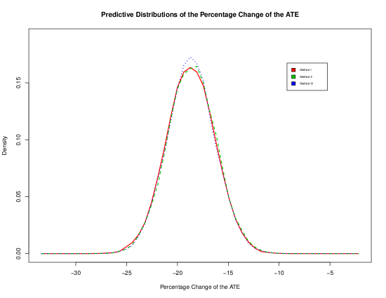
Figure 3: UK speed camera data.

References

- Antonelli et al. (2022) Antonelli, J., G. Papadogeorgou, and F. Dominici (2022). Causal inference in high dimensions: A marriage between Bayesian modeling and good frequentist properties. Biometrics 78(1), 100–114.
- Bernardo (1979) Bernardo, J. M. (1979). Reference posterior distributions for Bayesian inference. Journal of the Royal Statistical Society: Series B (Statistical Methodology) 41(2), 113–128.
- Bernardo and Smith (1994) Bernardo, J. M. and A. F. M. Smith (1994). Bayesian Theory. John Wiley & Sons.
- Berti et al. (2006) Berti, P., L. Pratelli, and P. Rigo (2006). Almost sure weak convergence of random probability measures. Stochastics and Stochastics Reports 78(2), 91–97.
- Bissiri et al. (2016) Bissiri, P. G., C. C. Holmes, and S. G. Walker (2016). A general framework for updating belief distributions. Journal of the Royal Statistical Society: Series B (Statistical Methodology) 78(5), 1103–1130.
- Bissiri and Walker (2019) Bissiri, P. G. and S. G. Walker (2019). On general Bayesian inference using loss functions. Statistics & Probability Letters 152, 89–91.
- Blackwell and MacQueen (1973) Blackwell, D. H. and J. B. MacQueen (1973). Ferguson distributions via Pólya urn schemes. The Annals of Statistics 1(2), 353–355.
- Chamberlain and Imbens (2003) Chamberlain, G. and G. W. Imbens (2003). Nonparametric applications of Bayesian inference. Journal of Business & Economic Statistics 21(1), 12–18.
- Chernozhukov et al. (2018) Chernozhukov, V., D. Chetverikov, M. Demirer, E. Duflo, C. Hansen, W. Newey, and J. Robins (2018). Double/debiased machine learning for treatment and structural parameters. The Econometrics Journal 21(1), C1–C68.
- Chernozhukov and Hong (2003) Chernozhukov, V. and H. Hong (2003). An MCMC approach to classical estimation. Journal of Econometrics 115(2), 293–346.
- Christie et al. (2003) Christie, S., R. A. Lyons, F. D. Dunstan, and S. J. Jones (2003). Are mobile speed cameras effective? A controlled before and after study. Injury Prevention 9(4), 302–306.
- Feigin and Tweedie (1989) Feigin, P. D. and R. L. Tweedie (1989). Linear functionals and Markov chains associated with Dirichlet processes. In Mathematical Proceedings of the Cambridge Philosophical Society, Volume 105, pp. 579–585. Cambridge University Press.
- Fong et al. (2021) Fong, E., C. C. Holmes, and S. G. Walker (2021). Martingale posterior distributions. arXiv: 2103.15671.
- Gains et al. (2004) Gains, A., B. Heydecker, J. Shrewsbury, and S. Robertson (2004). The national safety camera programme 3-year evaluation report. UK Department for Transport.
- Graham et al. (2016) Graham, D. J., E. J. McCoy, and D. A. Stephens (2016). Approximate Bayesian inference for doubly robust estimation. Bayesian Analysis 11(1), 47–69.
- Graham et al. (2019) Graham, D. J., C. Naik, E. J. McCoy, and H. Li (2019). Do speed cameras reduce road traffic collisions? PLoS One 14(9), e0221267.
- Grünwald and Van Ommen (2017) Grünwald, P. and T. Van Ommen (2017). Inconsistency of Bayesian inference for misspecified linear models, and a proposal for repairing it. Bayesian Analysis 12(4), 1069–1103.
- Hahn et al. (2020) Hahn, P. R., J. S. Murray, and C. M. Carvalho (2020). Bayesian regression tree models for causal inference: Regularization, confounding, and heterogeneous effects (with discussion). Bayesian Analysis 15(3), 965–1056.
- Ishwaran and Zarepour (2002) Ishwaran, H. and M. Zarepour (2002). Exact and approximate sum representations for the Dirichlet process. Canadian Journal of Statistics 30(2), 269–283.
- Jacob et al. (2017) Jacob, P. E., L. M. Murray, C. C. Holmes, and C. P. Robert (2017). Better together? Statistical learning in models made of modules. arXiv preprint arXiv:1708.08719.
- Jiang and Tanner (2008) Jiang, W. and M. A. Tanner (2008). Gibbs posterior for variable selection in high-dimensional classification and data mining. The Annals of Statistics 36(5), 2207–2231.
- Lijoi et al. (2004) Lijoi, A., I. Prünster, and S. G. Walker (2004). Extending Doob’s consistency theorem to nonparametric densities. Bernoulli 10(4), 651–663.
- Luo et al. (2023) Luo, Y., D. J. Graham, and E. J. McCoy (2023). Semiparametric Bayesian doubly robust causal estimation. Journal of Statistical Planning and Inference 225, 171–187.
- Lyddon et al. (2019) Lyddon, S. P., C. C. Holmes, and S. G. Walker (2019). General Bayesian updating and the loss-likelihood bootstrap. Biometrika 106(2), 465–478.
- McCandless et al. (2010) McCandless, L. C., I. J. Douglas, S. J. Evans, and L. Smeeth (2010). Cutting feedback in Bayesian regression adjustment for the propensity score. The International Journal of Biostatistics 6(2), 16.
- Monahan and Boos (1992) Monahan, J. F. and D. D. Boos (1992). Proper likelihoods for Bayesian analysis. Biometrika 79(2), 271–278.
- Muliere and Secchi (1996) Muliere, P. and P. Secchi (1996). Bayesian nonparametric predictive inference and bootstrap techniques. Annals of the Institute of Statistical Mathematics 48(4), 663–673.
- Muliere and Tardella (1998) Muliere, P. and L. Tardella (1998). Approximating distributions of random functionals of Ferguson-Dirichlet priors. Canadian Journal of Statistics 26(2), 283–297.
- Newton (1991) Newton, M. A. (1991). The weighted likelihood bootstrap and an algorithm for prepivoting. Ph. D. thesis, University of Washington.
- Newton et al. (2021) Newton, M. A., N. G. Polson, and J. Xu (2021). Weighted Bayesian bootstrap for scalable posterior distributions. Canadian Journal of Statistics 49(2), 421–437.
- Newton and Raftery (1994) Newton, M. A. and A. E. Raftery (1994). Approximate Bayesian inference with the weighted likelihood bootstrap. Journal of the Royal Statistical Society: Series B (Statistical Methodology) 56(1), 3–26.
- Quintana et al. (2020) Quintana, F. A., P. Mueller, A. Jara, and S. N. MacEachern (2020). The dependent Dirichlet process and related models. arXiv preprint arXiv:2007.06129.
- Robins et al. (1992) Robins, J. M., S. D. Mark, and W. K. Newey (1992). Estimating exposure effects by modelling the expectation of exposure conditional on confounders. Biometrics 48(2), 479–495.
- Rubin (1981) Rubin, D. B. (1981). The Bayesian bootstrap. The Annals of Statistics 9(1), 130–134.
- Saarela et al. (2016) Saarela, O., L. R. Belzile, and D. A. Stephens (2016). A Bayesian view of doubly robust causal inference. Biometrika 103(3), 667–681.
- Sethuraman (1994) Sethuraman, J. (1994). A constructive definition of Dirichlet priors. Statistica Sinica 4(2), 639–650.
- Stephens et al. (2022) Stephens, D. A., W. S. Nobre, E. E. M. Moodie, and A. M. Schmidt (2022). Causal inference under mis-specification: adjustment based on the propensity score. arXiv: 2201.12831. Accepted for publication, Bayesian Analysis.
- Syring and Martin (2019) Syring, N. and R. G. Martin (2019). Calibrating general posterior credible regions. Biometrika 106(2), 479–486.
- Wade (2013) Wade, S. (2013). Bayesian Nonparametric Regression Through Mixture Models. Ph. D. thesis, Bocconi University.
- Walker and Damien (2000) Walker, S. G. and P. Damien (2000). Representations of Lévy processes without Gaussian components. Biometrika 87(2), 477–483.
- Walker and Hjort (2001) Walker, S. G. and N. L. Hjort (2001). On Bayesian consistency. Journal of the Royal Statistical Society: Series B (Statistical Methodology) 63(4), 811–821.
- Zhang (2006) Zhang, T. (2006). From -entropy to KL-entropy: Analysis of minimum information complexity density estimation. The Annals of Statistics 34(5), 2180–2210.