A Block-Randomized Stochastic Method with Importance Sampling for CP Tensor Decomposition

Abstract

One popular way to compute the CANDECOMP/PARAFAC (CP) decomposition of a tensor is to transform the problem into a sequence of overdetermined least squares subproblems with Khatri-Rao product (KRP) structure involving factor matrices. In this work, based on choosing the factor matrix randomly, we propose a mini-batch stochastic gradient descent method with importance sampling for those special least squares subproblems. Two different sampling strategies are provided. They can avoid forming the full KRP explicitly and computing the corresponding probabilities directly. The adaptive step size version of the method is also given. For the proposed method, we present its detailed theoretical properties and comprehensive numerical performance. The results on synthetic and real data show that our method performs better than the corresponding one in the literature.

MSC Classification]15A69, 68W20, 90C52

1 Introduction

The CP decomposition of a tensor factorizes the tensor into a sum of $R$ rank-one tensors. That is, given an $N$-way tensor $\bm{\mathscr{{X}}}$ of size $I_{1}\times I_{2}\times\cdots\times I_{N}$, we wish to write it as:

$$\bm{\mathscr{{X}}}=\llbracket\mathbf{A}^{(1)},\mathbf{A}^{(2)},\cdots,\mathbf{A}^{(N)}\rrbracket=\sum_{r=1}^{R}\bm{a}^{(1)}_{r}\circ\bm{a}^{(2)}_{r}\circ\cdots\circ\bm{a}^{(N)}_{r},$$

where $R$ is a positive integer, $\bm{a}^{(n)}_{r}\in\mathbb{R}^{I_{n}}$, and $\mathbf{A}^{(n)}=[\bm{a}^{(n)}_{1},\bm{a}^{(n)}_{2},\cdots,\ \bm{a}^{(n)}_{R}]\in\mathbb{R}^{I_{n}\times R}$ for $n=1,\cdots,N$. Usually, $\mathbf{A}^{(n)}$ is called the $n$-th factor matrix. The CP decomposition is an important tool for data analysis and has found many important applications in some fields such as chemometrics, biogeochemistry, neuroscience, signal processing, and cyber traffic analysis; see e.g., kolda2009TensorDecompositions ; sidiropoulos2017TensorDecomposition .

It is well known that the computation of CP decomposition is a challenging problem. Currently, there are many methods for this decomposition. A popular one is the alternating least squares (ALS) method proposed in the original papers carroll1970AnalysisIndividual ; harshman1970FoundationsPARAFAC . Specifically, we transform the $n$-th factor matrix $\mathbf{A}^{(n)}$ as the solution to the following least squares problem:

$$\begin{gathered}\min_{\mathbf{A}\in\mathbb{R}^{I_{n}\times R}}\|\mathbf{Z}^{(n)}\mathbf{A}^{\intercal}-\mathbf{X}_{(n)}^{\intercal}\|_{F}^{2},\end{gathered}$$ (1)

where $\mathbf{Z}^{(n)}=\mathbf{A}^{(N)}\odot\cdots\odot\mathbf{A}^{(n+1)}\odot\mathbf{A}^{(n-1)}\odot\cdots\odot\mathbf{A}^{(1)}\in\mathbb{R}^{J_{n}\times R}$ with the symbol $\odot$ denoting the KRP, $\mathbf{X}_{(n)}\in\mathbb{R}^{I_{n}\times J_{n}}$ is the mode-$n$ unfolding of the input tensor $\bm{\mathscr{{X}}}$, and $J_{n}=\prod_{m=1,m\neq n}^{N}I_{m}$. Here, the mode-$n$ unfolding of a tensor means aligning the mode-$n$ fibers as the columns of an $I_{n}\times J_{n}$ matrix and the relation between the index of the tensor entry $x_{i_{1},i_{2},\cdots,i_{N}}$ and the index of the matrix entry $x_{i_{n},j}$ is

$$j=1+\sum_{k=1,k\neq n}^{N}(i_{k}-1)J^{\prime}_{k},$$ (2)

where $J^{\prime}_{k}=\prod_{m=1,m\neq n}^{k-1}I_{m}$. More symbol definitions are consistent with kolda2009TensorDecompositions .

As we know, the ALS method is the “workhorse” method for CP decomposition (CP-ALS). However, for large-scale problems, the cost of the method is prohibitive. To reduce the cost, Battaglino et al. battaglino2018PracticalRandomized applied random projection and uniform sampling techniques of the regular least squares problem drineas2011FasterLeast to (1) and designed the corresponding randomized algorithms in 2018. A main and attractive feature of the algorithms in battaglino2018PracticalRandomized is that they never explicitly form the full KPR matrices when applying projection and sampling. Later, building on the uniform sampling technique in battaglino2018PracticalRandomized , Fu et al. fu2020BlockRandomizedStochastic utilized the mini-batch stochastic gradient descent (SGD) method to solve the least squares subproblems in CP-ALS. This method was recently extended to the momentum version wang2021momentum . In 2020, Larsen and Kolda larsen2020PracticalLeverageBased performed the leverage-based sampling for (1) without forming the full KRP matrices and computing the corresponding probabilities directly. By the way, the method for estimating the leverage scores of the KRP matrix without forming it explicitly also appears in cheng2016SPALSFast . The random sampling methods introduced in battaglino2018PracticalRandomized ; fu2020BlockRandomizedStochastic ; larsen2020PracticalLeverageBased are built on fiber sampling. Besides, there are also some other random sampling algorithms for CP decomposition built on element sampling vervliet2014BreakingCurse ; bhojanapalli2015NewSampling ; vu2015NewStochastic or sub-tensor sampling beutel2014FlexiFaCTScalable ; vervliet2016RandomizedBlock . However, these two samplings are not suitable for the case of constraint fu2020BlockRandomizedStochastic .

Inspired by the doubly randomized computational framework in fu2020BlockRandomizedStochastic and the leverage-based sampling method in larsen2020PracticalLeverageBased , in this work, we present a mini-batch SGD method with importance sampling for CP decomposition. On the basis of the leverage scores or the squared Euclidean norms about rows of the KRP matrices, we propose two sampling strategies to select the mini-batch for the SGD method. As in larsen2020PracticalLeverageBased , these two strategies don’t need to form the KRP matrices explicitly and compute the corresponding probabilities directly either. Since the rows sampled by importance sampling contain more information compared to those by uniform sampling needell2016StochasticGradient , our new method can converge faster than the one from fu2020BlockRandomizedStochastic . Extensive numerical experiments validate this result.

The remainder of this paper is organized as follows. Section 2 provides some preliminaries. In Section 3, we present the sampling strategies and our method and its adaptive step size version. The relevant theoretical properties are given in Section 4. Section 5 is devoted to numerical experiments to illustrate our method. Finally, the concluding remarks of the whole paper are presented.

2 Preliminaries

We first introduce the idea on sampling the rows without forming the full KRP given in battaglino2018PracticalRandomized , that is, how to compute the sampled matrix $\mathbf{Z}^{(n)}(\mathcal{F}_{n},:)$ without explicitly forming $\mathbf{Z}^{(n)}$, where the set $\mathcal{F}_{n}\subset\{1,\cdots,J_{n}\}$ contains the indices of the rows sampled from $\mathbf{Z}^{(n)}$ and we will use the shorthand notation $\mathbf{Z}^{(n)}_{\mathcal{F}_{n}}=\mathbf{Z}^{(n)}(\mathcal{F}_{n},:)$ later in this paper. The idea mainly comes from the structure of $\mathbf{Z}^{(n)}$ and the definition of KRP, which make the rows of $\mathbf{Z}^{(n)}$ be written as the Hadamard product of the corresponding rows of the factor matrices, i.e.,

$$\mathbf{Z}^{(n)}(j,:) =\mathbf{A}^{(1)}(i_{1},:)\circledast\cdots\circledast\mathbf{A}^{(n-1)}(i_{n-1},:)$$

$$\quad\circledast\mathbf{A}^{(n+1)}(i_{n+1},:)\circledast\cdots\circledast\mathbf{A}^{(N)}(i_{N},:),$$ (3)

and the index $j$ and the multi-index $(i_{1},\cdots,i_{n-1},i_{n+1},\cdots,i_{N})$ be related as in (2). Based on the above fact, Battaglino et al. battaglino2018PracticalRandomized presented Algorithm 1 for computing $\mathbf{Z}^{(n)}_{\mathcal{F}_{n}}$, i.e., the sampled KRP (SKRP). The notation $\bm{idx}\in\mathbb{R}^{|\mathcal{F}_{n}|\times(N-1)}$ in Algorithm 1 represents the set of $|\mathcal{F}_{n}|$ multi-indices, that is, a row in $\bm{idx}$ represents a multi-index:

$$\{i_{1}^{(j)},\cdots,i_{n-1}^{(j)},i_{n+1}^{(j)},\cdots,i_{N}^{(j)}\}~{}~{}\text{with}~{}~{}j\in\mathcal{F}_{n}.$$ (4)

Here, we assume that these tuples are stacked in matrix form for efficiency. Thus, each multiplicand $\mathbf{A}_{|\mathcal{F}_{n}|}^{(n)}$ is of size $|\mathcal{F}_{n}|\times R$. Furthermore, Algorithm 1 also presents how to compute $\mathbf{X}_{(n)}^{\mathcal{F}_{n}}=\mathbf{X}_{(n)}^{\intercal}(\mathcal{F}_{n},:)=\mathbf{X}_{(n)}(:,\mathcal{F}_{n})$ given $\bm{idx}$. Note that, to find $\mathbf{Z}^{(n)}_{\mathcal{F}_{n}}$ and $\mathbf{X}_{(n)}^{\mathcal{F}_{n}}$, we don’t need to form ${\mathcal{F}_{n}}$ explicitly either.

Algorithm 1 SKRP and Sampled tensor fibers (SKRP-ST) battaglino2018PracticalRandomized

1:function $[\mathbf{Z}^{(n)}_{\mathcal{F}_{n}},\mathbf{X}_{(n)}^{\mathcal{F}_{n}}]$ = SKRP-ST($n$, $\bm{idx}$, $\{\mathbf{A}^{(k)}\}_{k=1,k\neq n}^{N}$)

2:    $\mathbf{Z}^{(n)}_{\mathcal{F}_{n}}\leftarrow\textbf{1}$ $\ignorespaces\triangleright$ $\textbf{1}\in\mathbb{R}^{|\mathcal{F}_{n}|\times R}$ a matrix with all elements 1

3:    for $m=1,\cdots,n-1,n+1,\cdots,N$ do

4:        $\mathbf{A}_{|\mathcal{F}_{n}|}^{(m)}\leftarrow\mathbf{A}^{(m)}(\bm{idx}(:,m),:)$

5:        $\mathbf{Z}^{(n)}_{\mathcal{F}_{n}}\leftarrow\mathbf{Z}^{(n)}_{\mathcal{F}_{n}}\circledast\mathbf{A}_{|\mathcal{F}_{n}|}^{(m)}$

6:    end for

7:    $\bm{\mathscr{{X}}}^{\mathcal{F}_{n}}\leftarrow\bm{\mathscr{{X}}}(\bm{idx}(:,1),\cdots,\bm{\mathscr{{X}}}(\bm{idx}(:,n-1),:,\bm{\mathscr{{X}}}(\bm{idx}(:,n+1),\cdots,\bm{\mathscr{{X}}}(\bm{idx}(:,N))$

8:    $\mathbf{X}_{(n)}^{\mathcal{F}_{n}}\leftarrow$ Unfolding($\bm{\mathscr{{X}}}^{\mathcal{F}_{n}}$, $n$)

9:    return $\mathbf{Z}^{(n)}_{\mathcal{F}_{n}},\mathbf{X}_{(n)}^{\mathcal{F}_{n}}$

10:end function

Combining Algorithm 1 with uniform sampling, i.e., the indices in each column of $\bm{idx}$ are sampled from the corresponding index set uniformly, and the SGD method, Fu et al. fu2020BlockRandomizedStochastic proposed the Block-Randomized SGD for CP Decomposition (BrasCPD), where the block-randomized means choosing the factor matrix, i.e., sampling a mode from all modes, randomly. Specifically, the authors first rewrite the CP decomposition of a tensor as the following optimization problem:

$$\min_{\{\mathbf{A}^{(n)}\in\mathbb{R}^{I_{n}\times R}\}_{n=1}^{N}}~{}f(\mathbf{A}^{(1)},\cdots,\mathbf{A}^{(N)}),$$ (5)

where

$$f(\mathbf{A}^{(1)},\cdots,\mathbf{A}^{(N)}) =\frac{1}{2}\|\bm{\mathscr{{X}}}-\llbracket\mathbf{A}^{(1)},\mathbf{A}^{(2)},\cdots,\mathbf{A}^{(N)}\rrbracket\|_{F}^{2}$$

$$=\frac{1}{2}\|\mathbf{Z}^{(n)}(\mathbf{A}^{(n)})^{\intercal}-\mathbf{X}_{(n)}^{\intercal}\|_{F}^{2}.$$

Then, by choosing a mode randomly and obtaining $\mathbf{Z}^{(n)}_{\mathcal{F}_{n}}$ and $\mathbf{X}_{(n)}^{\mathcal{F}_{n}}$ using Algorithm 1 with uniform sampling, with the GD method, they update the latent factor of the sampled least squares problem of (1), i.e.,

$$\mathbf{A}^{(n)}\leftarrow\arg\min_{\mathbf{A}\in\mathbb{R}^{I_{n}\times R}}\|\mathbf{Z}^{(n)}_{\mathcal{F}_{n}}\mathbf{A}^{\intercal}-\mathbf{X}_{(n)}^{\mathcal{F}_{n}}\|_{F}^{2},$$ (6)

by

$$\mathbf{A}^{(n)}_{(t+1)}\leftarrow\mathbf{A}^{(n)}_{(t)}-\frac{\alpha_{t}}{|\mathcal{F}_{n}|}\left(\mathbf{A}^{(n)}_{(t)}(\mathbf{Z}^{(n)}_{\mathcal{F}_{n}})^{\intercal}\mathbf{Z}^{(n)}_{\mathcal{F}_{n}}-\mathbf{X}_{(n)}^{\mathcal{F}_{n}}\mathbf{Z}^{(n)}_{\mathcal{F}_{n}}\right).$$

The specific algorithm is listed in Algorithm 2.

Algorithm 2 BrasCPD fu2020BlockRandomizedStochastic

1:function $\{\mathbf{A}^{(n)}\}_{n=1}^{N}$= BrasCPD($\bm{\mathscr{{X}}},R,|\mathcal{F}_{n}|,\{\mathbf{A}^{(n)}_{(0)}\}_{n=1}^{N},\{\alpha^{t}\}$) $\ignorespaces\triangleright$ $N$-way tensor $\bm{\mathscr{{X}}}\in\mathbb{R}^{I_{1}\times\cdots\times I_{N}}$; $\ignorespaces\triangleright$ rank $R$, sample size $|\mathcal{F}_{n}|$; $\ignorespaces\triangleright$ initialization $\{\mathbf{A}^{(n)}_{(0)}\}_{n=1}^{N}$, step size $\{\alpha^{t}\}_{t=0,1,\cdots}$

2:    $t\leftarrow 0$

3:    repeat

4:        Uniformly sample $n$ from $\{1,\cdots,N\}$

5:         Sample $\mathcal{F}_{n}$ uniformly from $\{1,\cdots,J_{n}\}$

6:        Compute $\mathbf{G}^{(n)}_{(t)}=\frac{1}{|\mathcal{F}_{n}|}\left(\mathbf{A}^{(n)}_{(t)}(\mathbf{Z}^{(n)}_{\mathcal{F}_{n}})^{\intercal}\mathbf{Z}^{(n)}_{\mathcal{F}_{n}}-\mathbf{X}_{(n)}^{\mathcal{F}_{n}}\mathbf{Z}^{(n)}_{\mathcal{F}_{n}}\right)$

7:        Update $\mathbf{A}^{(n)}_{(t+1)}\leftarrow\mathbf{A}^{(n)}_{(t)}-\alpha_{t}\mathbf{G}^{(n)}_{(t)}$, and $\mathbf{A}^{(n^{\prime})}_{(t+1)}\leftarrow\mathbf{A}^{(n^{\prime})}_{(t)}$ for $n^{\prime}\neq n$

8:        $t\leftarrow t+1$

9:    until some stopping criterion is reached

10:    return $\{\mathbf{A}^{(n)}\}_{n=1}^{N}$

11:end function

In addition, the following two definitions are also necessary throughout the rest of this paper.

Definition 1.

We say $\bm{p}\in[0,1]^{N}$, i.e., an $N$ dimensional vector with the entries being in $[0,1]$, is a probability distribution if $\sum_{i=1}^{N}p_{i}=1$.

Definition 2.

For a random variable $\xi\in[N]$, we say $\xi\sim\text{\sc multinomial}(\bm{p})$ if $\bm{p}\in[0,1]^{N}$ is a probability distribution and ${\sf Pr}(\xi=i)=p_{i}$.

3 Sampling Strategies and Proposed Method

In this section, we first present two importance sampling strategies to select the mini-batch for SGD method based on the leverage scores or the squared Euclidean norms about rows of the KRP matrix, and then present the doubly randomized variant of CP-ALS. Moreover, its adaptive step size version is also presented, which can eliminate the challenges in adjusting the parameters and the non-convergence of the algorithm owing to improper step sizes.

3.1 Sampling strategies

We begin with some definitions.

Definition 3 (Leverage Scores drineas2012FastApproximation ).

Let $\mathbf{A}\in\mathbb{R}^{m\times n}$ with $m>n$, and let $\mathbf{Q}\in\mathbb{R}^{m\times n}$ be any orthogonal basis for the column space of $\mathbf{A}$. The leverage score of the $i$-th row of $\mathbf{A}$ is given by

$$\ell_{i}(\mathbf{A})=\|\mathbf{Q}(i,:)\|_{2}^{2}.$$

Definition 4 (Leveraged-based Probability Distribution woodruff2014SketchingTool ).

Let $\mathbf{A}\in\mathbb{R}^{m\times n}$ with $m>n$. We say a probability distribution $\bm{p}=[p_{1},\cdots,p_{m}]^{\intercal}$ is a leveraged-based probability distribution for $\mathbf{A}$ if $p_{i}\geq\beta\frac{\ell_{i}(\mathbf{A})}{n}$ with $0<\beta\leq 1$ and $i\in[m]$.

Definition 5 (Euclidean-based Probability Distribution).

Let $\mathbf{A}\in\mathbb{R}^{m\times n}$ with $m>n$. We say a probability distribution $\bm{p}=[p_{1},\cdots,p_{m}]^{\intercal}$ is an Euclidean-based probability distribution for $\mathbf{A}$ if $p_{i}\geq\beta\|\mathbf{A}(i,:)\|^{2}_{2}/\|\mathbf{A}\|_{F}^{2}$ with $0<\beta\leq 1$ and $i\in[m]$.

Since it is expensive to compute the leverage scores of a KRP matrix directly, Cheng et al. cheng2016SPALSFast presented their upper bounds.

Lemma 1 (Leverage Score Bound for KRP Matrix cheng2016SPALSFast ).

For matrices $\mathbf{A}^{(k)}\in\mathbb{R}^{I_{k}\times R}$ with $I_{k}>R$ for $k=1,\cdots,K$, let $\ell_{i_{k}}$ be the leverage score of the $i_{k}$-th row of $\mathbf{A}^{(k)}$. Then, for the KRP matrix $\mathbf{Z}=\mathbf{A}^{(1)}\odot\mathbf{A}^{(2)}\odot\cdots\odot\mathbf{A}^{(K)}$, the leverage score $\ell_{i_{1},\cdots,i_{K}}$ of its $j$-th row corresponding to $\{i_{1},\cdots,i_{K}\}$ satisfies

$$\ell_{i_{1},\cdots,i_{K}}\leq\prod_{k=1}^{K}\ell_{i_{k}}.$$

Hence, the leveraged-based sampling probability for the $j$-th row of the above KRP matrix can be set to be

$$p_{j}=\frac{1}{R^{K}}\prod_{k=1}^{K}\ell_{i_{k}}.$$ (7)

In this case, $\beta$ in Definition 4 is equal to $1/R^{K-1}$. Furthermore, Larsen and Kolda larsen2020PracticalLeverageBased showed that sampling the $j$-th row of $\mathbf{Z}$ with the above probability can be carried out by sampling the corresponding rows from factor matrices with suitable probabilities independently. The specific result is given in the following lemma.

Lemma 2 (larsen2020PracticalLeverageBased ).

Let $\mathbf{A}^{(k)}\in\mathbb{R}^{I_{k}\times R}$ for $k=1,\cdots,K$, and $\bm{\ell}(\mathbf{A}^{(k)})$ be the vector of leverage scores for $\mathbf{A}^{(k)}$. Let

$$i_{k}\sim\text{\sc multinomial}(\bm{\ell}(\mathbf{A}^{(k)})/R)~{}~{}\text{for}~{}~{}k=1,\cdots,K.$$

Then, the probability of selecting the multi-index $\{i_{1},\cdots,i_{K}\}$ is $p_{j}$ in (7).

For the case on the squared Euclidean norms, we have the similar conclusions. That is, the Euclidean-based sampling probability for the $j$-th row of the above KRP matrix can be set to be

$$p_{j}=\prod_{k=1}^{K}\frac{\|\mathbf{A}^{(k)}(i_{k},:)\|^{2}_{2}}{\|\mathbf{A}^{(k)}\|_{F}^{2}},$$ (8)

and to sample the $j$-th row of $\mathbf{Z}$ with the above probability, it suffices to sample the corresponding rows from factor matrices with suitable probabilities independently. These conclusions are guaranteed by the following two lemmas, whose proofs are similar to those of Lemmas 1 and 2. So we omit them here.

Lemma 3.

Let $\mathbf{A}^{(k)}\in\mathbb{R}^{I_{k}\times R}$ with $I_{k}>R$ for $k=1,\cdots,K$. For the KRP matrix $\mathbf{Z}=\mathbf{A}^{(1)}\odot\mathbf{A}^{(2)}\odot\cdots\odot\mathbf{A}^{(K)}$, the squared Euclidean norms of its $j$-th row corresponding to $\{i_{1},\cdots,i_{K}\}$ satisfies

$$\|\mathbf{Z}(j,:)\|^{2}_{2}\leq\prod_{k=1}^{K}\|\mathbf{A}^{(k)}(i_{k},:)\|^{2}_{2}.$$

Lemma 4.

Let $\mathbf{A}^{(k)}\in\mathbb{R}^{I_{k}\times R}$ for $k=1,\cdots,K$, and $\bm{p}_{k}$ be the Euclidean-based probability distribution for $\mathbf{A}^{(k)}$ with $\beta=1$, i.e., $\bm{p}_{k}(i)=\|\mathbf{A}^{(k)}(i,:)\|^{2}_{2}/\|\mathbf{A}^{(k)}\|_{F}^{2}$ with $i\in[I_{k}]$. Let

$$i_{k}\sim\text{\sc multinomial}(\bm{p}_{k})~{}~{}\text{for}~{}~{}k=1,\cdots,K.$$

Then, the probability of selecting the multi-index $\{i_{1},\cdots,i_{K}\}$ is $p_{j}$ in (8).

In the following, we introduce how to find the mini-batches and compute their sampling probabilities based on the above Leveraged-based and Euclidean-based probability distributions, respectively.

We first sample $|\mathcal{F}_{n}|$ rows from each $\{\mathbf{A}^{(k)}\}_{k=1,k\neq n}^{N}$ using the leveraged-based probability distribution for $\mathbf{A}^{(k)}$ with $\beta=1$, i.e., $\bm{p}_{k}=\frac{\bm{\ell}(\mathbf{A}^{(k)})}{R}$. Thus, we can get the $\bm{idx}$:

$$\begin{bmatrix}\{i_{1}^{(j_{1})}&\cdots&i_{n-1}^{(j_{1})}&i_{n+1}^{(j_{1})}&\cdots&i_{N}^{(j_{1})}\}\\ \{i_{1}^{(j_{2})}&\cdots&i_{n-1}^{(j_{2})}&i_{n+1}^{(j_{2})}&\cdots&i_{N}^{(j_{2})}\}\\ \vdots&\vdots&\vdots&\vdots&\vdots&\vdots\\ \{i_{1}^{(j_{|\mathcal{F}_{n}|})}&\cdots&i_{n-1}^{(j_{|\mathcal{F}_{n}|})}&i_{n+1}^{(j_{|\mathcal{F}_{n}|})}&\cdots&i_{N}^{(j_{|\mathcal{F}_{n}|})}\}\\ \end{bmatrix}.$$ (9)

Then, based on the above set of tuples, using (2) and Lemma 2, we can obtain the index set $\mathcal{F}_{n}=\{j_{1},j_{2},\cdots,j_{|\mathcal{F}_{n}|}\}$ of the sampled $|\mathcal{F}_{n}|$ rows of $\mathbf{Z}^{(n)}$, and the corresponding sampling probabilities

$$\bm{p}_{\mathcal{F}_{n}}=[p_{j_{1}},\cdots,p_{j_{|\mathcal{F}_{n}|}}]^{\intercal},$$ (10)

where $p_{j_{f}}=\frac{\bar{\ell}_{j_{f}}(\mathbf{Z}^{(n)})}{R^{N-1}}$ and $\bar{\ell}_{j_{f}}(\mathbf{Z}^{(n)})=\prod_{k=1,k\neq n}^{N}\ell_{i_{k}^{(j_{f})}}(\mathbf{A}^{(k)})$. Moreover, with the above $\bm{idx}$, we can find $\mathbf{Z}^{(n)}_{\mathcal{F}_{n}}$ and $\mathbf{X}_{(n)}^{\mathcal{F}_{n}}$ using Algorithm 1.

The procedure for the case on the Euclidean-based probability distribution is similar except that the above $\bm{p}_{k}$ is replaced by $\bm{p}_{k}$ in Lemma 4 and the above $p_{j_{f}}$ is replaced by $p_{j_{f}}=\prod_{k=1,k\neq n}^{N}\frac{\|\mathbf{A}^{(k)}(i_{k}^{(j_{f})},:)\|^{2}_{2}}{\|\mathbf{A}^{(k)}\|_{F}^{2}}$.

Based on the above discussions, we have the following algorithmic framework, i.e., Algorithm 3.

Algorithm 3 SKRP-ST with importance sampling (SKRP-ST-I)

1:function $[\mathbf{Z}^{(n)}_{\mathcal{F}_{n}},\mathbf{X}_{(n)}^{\mathcal{F}_{n}},\bm{p}_{\mathcal{F}_{n}}]$ = SKRP-ST-I($n$, $|\mathcal{F}_{n}|$, $\{\bm{p}_{k}\}_{k=1,k\neq n}^{N},\{\mathbf{A}^{(k)}\}_{k=1,k\neq n}^{N}$)

2:    for $k=1,\cdots,n-1,n+1,\cdots,N$ do

3:        $\bm{idx}(:,k)=$ Randsample($I_{k},|\mathcal{F}_{n}|,true,\bm{p}_{k}$)

4:    end for

5:    $[\mathbf{Z}^{(n)}_{\mathcal{F}_{n}},\mathbf{X}_{(n)}^{\mathcal{F}_{n}}]$ = SKRP-ST($n$, $\bm{idx}$, $\{\mathbf{A}^{(k)}\}_{k=1,k\neq n}^{N}$)

6:    $\bm{p}_{\mathcal{F}_{n}}\leftarrow$ (10) with leveraged/Euclidean-based probability distribution

7:    return $\mathbf{Z}^{(n)}_{\mathcal{F}_{n}},\mathbf{X}_{(n)}^{\mathcal{F}_{n}},\bm{p}_{\mathcal{F}_{n}}$

8:end function

Remark 1.

The two importance sampling probability distributions considered above are empirical. In Theorem 11 below, we will present a theoretical optimal one. In addition, the mini-batches here are constructed by sampling rows first and then combining them into blocks. We can also obtain them by blocking the rows first and then sampling blocks.

3.2 Proposed method

We first give the stochastic gradient $\mathbf{G}^{(n)}_{(t)}$, corresponding to the sampling strategies described in Section 3.1,

$$\mathbf{G}^{(n)}_{(t)}=\frac{1}{|\mathcal{F}_{n}|J_{n}}\left(\mathbf{A}^{(n)}_{(t)}(\mathbf{D}(\mathbf{Z}^{(n)}_{\mathcal{F}_{n}})^{\intercal})\mathbf{Z}^{(n)}_{\mathcal{F}_{n}}-\mathbf{D}\mathbf{X}_{(n)}^{\mathcal{F}_{n}}\mathbf{Z}^{(n)}_{\mathcal{F}_{n}}\right),$$ (11)

where $\mathbf{D}={\operatorname{diag}}[\frac{1}{p_{j_{1}}},\cdots,\frac{1}{p_{j_{|\mathcal{F}_{n}|}}}]$ is from (10). Then, the latent factor matrices can be updated by

$$\mathbf{A}^{(n)}_{(t+1)}\leftarrow\mathbf{A}^{(n)}_{(t)}-\alpha_{t}\mathbf{G}^{(n)}_{(t)},~{}~{}n=1,\cdots,N.$$ (12)

Therefore, we can propose our method in Algorithm 4. Like fu2020BlockRandomizedStochastic , we call it Block-Randomized Weighted SGD for CPD (BrawsCPD). Similarly, we call the BrawsCPD with the two sampling strategies in Section 3.1 the LBrawsCPD and EBrawsCPD, respectively.

Algorithm 4 BrawsCPD

1:function $\{\mathbf{A}^{(n)}\}_{n=1}^{N}$= BrawsCPD($\bm{\mathscr{{X}}},R,|\mathcal{F}_{n}|,\{\mathbf{A}^{(n)}_{(0)}\}_{n=1}^{N},\{\alpha_{t}\}$)

2:    $t\leftarrow 0$

3:    repeat

4:        Uniformly sample $n$ from $\{1,\cdots,N\}$

5:        $[\mathbf{Z}^{(n)}_{\mathcal{F}_{n}},\mathbf{X}_{(n)}^{\mathcal{F}_{n}},\bm{p}_{\mathcal{F}_{n}}]$ = SKRP-ST-I($n$, $|\mathcal{F}_{n}|$, $\{\bm{p}_{k}\}_{k=1,k\neq n}^{N}$, $\{\mathbf{A}^{(N)}\}_{k=1,k\neq n}^{N}$)

6:        Form the stochastic gradient $\mathbf{G}^{(n)}_{(t)}\leftarrow$ (11)

7:        Update $\mathbf{A}^{(n)}_{(t+1)}\leftarrow\eqref{eq:proposed}$, $\mathbf{A}^{(n^{\prime})}_{(t+1)}\leftarrow\mathbf{A}^{(n^{\prime})}_{(t)}$ for $n^{\prime}\neq n$

8:        $t\leftarrow t+1$

9:    until some stopping criterion is reached

10:    return $\{\mathbf{A}^{(n)}\}_{n=1}^{N}$

11:end function

To avoid running the step size schedule, similar to fu2020BlockRandomizedStochastic , we also give an adaptive step size scheme with the following updating rule:

$$[\bm{\eta}_{(t)}^{(n)}]_{i,r} \leftarrow\frac{\eta}{\left(b+\sum_{t^{\prime}=1}^{t}[\mathbf{G}^{(n)}_{(t)}]_{i,r}^{2}\right)^{1/2}},~{}~{}i\in[I_{n}],~{}r\in[R],$$ (13a)

$$\mathbf{A}^{(n)}_{(t+1)} \leftarrow\mathbf{A}^{(n)}_{(t)}-\bm{\eta}_{(t)}^{(n)}\circledast\mathbf{G}^{(n)}_{(t)},$$ (13b)

$$\mathbf{A}^{(n^{\prime})}_{(t+1)} \leftarrow\mathbf{A}^{(n^{\prime})}_{(t)},~{}~{}n^{\prime}\neq n,$$ (13c)

where $\eta,b>0$. Here, $b>0$ is introduced to prevent division by zero. In practice, setting $b=0$ does not hurt the performance. We summary the corresponding algorithm in Algorithm 5, which is named as AdawsCPD. Meanwhile, we name the AdawsCPD with the two sampling strategies in Section 3.1 the LAdawsCPD and EAdawsCPD, respectively.

Algorithm 5 AdawsCPD

1:function $\{\mathbf{A}^{(n)}\}_{n=1}^{N}$= AdawsCPD($\bm{\mathscr{{X}}},R,{|\mathcal{F}_{n}|},\{\mathbf{A}^{(n)}_{(0)}\}_{n=1}^{N}$)

2:    $t\leftarrow 0$

3:    repeat

4:        Uniformly sample $n$ from $\{1,\cdots,N\}$

5:        $[\mathbf{Z}^{(n)}_{\mathcal{F}_{n}},\mathbf{X}_{(n)}^{\mathcal{F}_{n}},\bm{p}_{\mathcal{F}_{n}}]$ = SKRP-ST-I($n$, $|\mathcal{F}_{n}|$, $\{\bm{p}_{k}\}_{k=1,k\neq n}^{N}$, $\{\mathbf{A}^{(N)}\}_{k=1,k\neq n}^{N}$)

6:        Form the stochastic gradient $\mathbf{G}^{(n)}_{(t)}\leftarrow$ (11)

7:        Determine the step size $\bm{\eta}_{(t)}^{(n)}\leftarrow$ (13a)

8:        Update $\mathbf{A}^{(n)}_{(t+1)}\leftarrow$ (13b), $\mathbf{A}^{(n^{\prime})}_{(t+1)}\leftarrow\mathbf{A}^{(n^{\prime})}_{(t)}$ for $n^{\prime}\neq n$

9:        $t\leftarrow t+1$

10:    until some stopping criterion is reached

11:    return $\{\mathbf{A}^{(n)}\}_{n=1}^{N}$

12:end function

4 Theoretical Properties

In this section, we provide some theoretical results of the proposed method, which mainly include the unbiasedness of stochastic gradient, the error analysis of method, and the analysis on variance of stochastic gradient. For simplicity, we will often use the shorthand notation $f(\bm{\theta})$ to denote $f(\mathbf{A}^{(1)},\cdots,\mathbf{A}^{(N)})$, where $\bm{\theta}=[\mathbf{A}^{(1)},\cdots,\mathbf{A}^{(N)}]$. Thus, considering the definition of Frobenius norm, (5) can be rewritten as

$$\min_{\{\mathbf{A}^{(n)}\in\mathbb{R}^{I_{n}\times R}\}_{n=1}^{N}}~{}(1/J_{n})~{}\sum_{i}f_{i}\left(\bm{\theta}\right),$$ (14)

where $f_{i}(\bm{\theta})=\frac{J_{n}}{2}\|\mathbf{Z}^{(n)}(i,:)\mathbf{A}^{\intercal}-\mathbf{X}_{(n)}^{\intercal}(i,:)\|^{2}_{F}$.

4.1 Unbiasedness of stochastic gradient

For convenience, we define $\xi_{(t)}\in\{1,\cdots,N\}$ and $\zeta_{(t)}\subseteq\{1,\cdots,J_{\xi_{(t)}}\}$ as the random variables (r.v.s) responsible for selecting the mode and fibers in the $t$-th iteration, respectively.

Theorem 5 (Unbiased Gradient).

Denote $\mathcal{B}_{(t)}$ as the filtration generated by the r.v.s

$$\{\xi_{(0)},\zeta_{(0)},\xi_{(1)},\zeta_{(1)},\cdots,\xi_{(t-1)},\zeta_{(t-1)}\}$$

such that the $t$-th iteration $\bm{\theta}_{(t)}$ is determined conditioned on $\mathcal{B}_{(t)}$. Then the stochastic gradient in (11) is the unbiased estimate of the full gradient with respect to (w.r.t.) $\mathbf{A}^{(\xi_{(t)})}$, i.e.,

$$\mathbb{E}_{\zeta_{(t)}}\left[\mathbf{G}^{(\xi_{(t)})}_{(t)}~{}|~{}\mathcal{B}_{(t)},\xi_{(t)}\right]=\nabla_{\mathbf{A}^{(\xi_{(t)})}}f({\bm{\theta}}_{(t)}).$$ (15)

Proof: Note that the stochastic gradient in (11) can be rewritten as

$$\mathbf{G}^{(n)}_{(t)} =\frac{1}{|\mathcal{F}_{n}|J_{n}}\sum_{f=1}^{|\mathcal{F}_{n}|}\frac{1}{p_{j_{f}}}\nabla_{\mathbf{A}^{(n)}}f_{j_{f}}(\bm{\theta}_{(t)}).$$

Hence, we have

$$\mathbb{E}_{\zeta_{(t)}}\left[\mathbf{G}^{(\xi_{(t)})}_{(t)}~{}|~{}\mathcal{B}_{(t)},\xi_{(t)}\right] =\frac{1}{|\mathcal{F}_{n}|J_{n}}\sum_{f=1}^{|\mathcal{F}_{n}|}\mathbb{E}\left(\frac{1}{p_{j_{f}}}\nabla_{\mathbf{A}^{(\xi_{(t)})}}f_{j_{f}}(\bm{\theta}_{(t)})\right)$$

$$=\frac{1}{|\mathcal{F}_{n}|J_{n}}\sum_{f=1}^{|\mathcal{F}_{n}|}\sum_{j_{f}\in[J_{n}]}\left(\frac{1}{p_{j_{f}}}p_{j_{f}}\nabla_{\mathbf{A}^{(\xi_{(t)})}}f_{j_{f}}(\bm{\theta}_{(t)})\right)$$

$$=\frac{1}{J_{n}}\sum_{j_{f}\in[J_{n}]}\nabla_{\mathbf{A}^{(\xi_{(t)})}}f_{j_{f}}(\bm{\theta}_{(t)})=\nabla_{\mathbf{A}^{(\xi_{(t)})}}f(\bm{\theta}_{(t)}).$$

So, the desired result holds.

Remark 2.

Based on the unbiasedness of the stochastic gradient given in (11), under some assumptions presented in fu2020BlockRandomizedStochastic , along the same line of proofs of Propositions 1 and 3 in fu2020BlockRandomizedStochastic , we can show that the solution sequence produced by BrawsCPD satisfies

$$\liminf_{t\rightarrow\infty}\mathbb{E}\left[\|\nabla f(\bm{\theta}_{(t)})\|_{F}^{2}\right]=0,$$

and the solution sequence produced by AdawsCPD satisfies

$${\sf Pr}\left(\liminf_{t\rightarrow\infty}\|\nabla f(\bm{\theta}_{(t)})\|_{F}^{2}=0\right)=1.$$

That is, these sequences converge to the corresponding stationary points.

4.2 Error analysis

To investigate the error analysis of the proposed method, we need some preparations. They are presented in the following two lemmas, which are mainly from the facts that the objective function $f(\bm{\theta})$ is block multiconvex xu2013BlockCoordinate and has block-wise Lipschitz continuous gradient fu2020BlockRandomizedStochastic . This is because $f(\bm{\theta})$ w.r.t. $\mathbf{A}^{(n)}$ is a plain least squares fitting criterion.

Lemma 6 (Block Multiconvex xu2013BlockCoordinate ).

Suppose that $\mathbf{Z}^{(n)}$ has full column rank. Then, for $\hat{\bm{\theta}}$, $\bar{\bm{\theta}}$ and the mode $n\in\{1,\cdots,N\}$, there exists a constant $\mu^{(n)}$ such that

$$f(\hat{\bm{\theta}})\geq f(\bar{\bm{\theta}})+\left<\nabla_{\mathbf{A}^{(n)}}f(\bar{\bm{\theta}}),\hat{\mathbf{A}}^{(n)}-\bar{\mathbf{A}}^{(n)}\right>+\frac{\mu^{(n)}}{2}\|\hat{\mathbf{A}}^{(n)}-\bar{\mathbf{A}}^{(n)}\|_{F}^{2},$$

where $\hat{\bm{\theta}}$ and $\bar{\bm{\theta}}$ are the same except the $n$-th factor, i.e., $\hat{\mathbf{A}}^{(i)}=\bar{\mathbf{A}}^{(i)}$ for $i\neq n$.

Lemma 7 (Block-wise Lipschitz Continuous Gradient fu2020BlockRandomizedStochastic ).

For $\hat{\bm{\theta}}$, $\bar{\bm{\theta}}$ and the mode $n\in\{1,\cdots,N\}$, there exists a constant $L^{(n)}$ such that

$$f(\hat{\bm{\theta}})\leq f(\bar{\bm{\theta}})+\left<\nabla_{\mathbf{A}^{(n)}}f(\bar{\bm{\theta}}),\hat{\mathbf{A}}^{(n)}-\bar{\mathbf{A}}^{(n)}\right>+\frac{L^{(n)}}{2}\|\hat{\mathbf{A}}^{(n)}-\bar{\mathbf{A}}^{(n)}\|_{F}^{2},$$

where $\hat{\bm{\theta}}$ and $\bar{\bm{\theta}}$ are the same except the $n$-th factor, i.e., $\hat{\mathbf{A}}^{(i)}=\bar{\mathbf{A}}^{(i)}$ for $i\neq n$.

Remark 3.

It is well known that $\mu^{(n)}$ and $L^{(n)}$ can be chosen as $\lambda_{\min}((\mathbf{Z}^{(n)})^{\intercal}\mathbf{Z}^{(n)})$ and $\lambda_{\max}((\mathbf{Z}^{(n)})^{\intercal}\mathbf{Z}^{(n)})$, respectively. In addition, the assumption of Lemma 6 can always be satisfied in our problem, and by the monotonicity of strongly convex function, we have

$$\left<\nabla_{\mathbf{A}^{(n)}}f(\hat{\bm{\theta}})-\nabla_{\mathbf{A}^{(n)}}f(\bar{\bm{\theta}}),\hat{\mathbf{A}}^{(n)}-\bar{\mathbf{A}}^{(n)}\right>\geq\mu^{(n)}\|\hat{\mathbf{A}}^{(n)}-\bar{\mathbf{A}}^{(n)}\|_{F}^{2}.$$ (16)

Theorem 8 (Main Theorem).

Let $\mathbf{A}_{*}^{(n)}$ for $n=1,\cdots,N$ be the factor matrices derived by the regular CP-ALS, $\bm{\mathscr{{X}}}_{*}=\llbracket\mathbf{A}_{*}^{(1)},\mathbf{A}_{*}^{(2)},\cdots,\mathbf{A}_{*}^{(N)}\rrbracket$ and $\bm{\mathscr{{X}}}_{true}$ be the true data tensor. Suppose that the updates $\mathbf{A}^{(n)}_{(t)}$ are bounded for all $n,t$, and the step size $\alpha_{t}$ is fixed as $\alpha$ satisfying $0<\alpha<\frac{1}{2\mu}$ with $\mu$ being a constant. Then, after $T$ iterations, the solution sequence produced by BrawsCPD satisfies:

$$\mathbb{E}\left[\|\llbracket\mathbf{A}^{(1)}_{(T)},\mathbf{A}^{(2)}_{(T)},\cdots,\mathbf{A}^{(N)}_{(T)}\rrbracket-\bm{\mathscr{{X}}}_{true}\|_{F}^{2}\right] \leq\frac{L}{4}\left[(1-2\alpha\mu)^{T}\Delta_{0}^{2}+\frac{\alpha M}{2\mu}\right]$$

$$\qquad+\frac{1}{2}\|\bm{\mathscr{{X}}}_{*}-\bm{\mathscr{{X}}}_{true}\|_{F}^{2},$$ (17)

where $L$ is a constant, $\Delta_{t}=\|\mathbf{A}_{(t)}^{(\xi_{(t)})}-\mathbf{A}_{*}^{(\xi_{(t)})}\|_{F}$, and

$$M=\max\left\{\mathbb{E}_{\zeta_{(t)}}\left[\|\mathbf{G}^{(\xi_{(t)})}_{(t)}\|_{F}^{2}~{}|~{}\mathcal{B}_{(t)},\xi_{(t)}\right]\right\}$$

with $\mathcal{B}_{(t)}$, $\xi_{(t)}$ and $\zeta_{(t)}$ being defined as in Section 4.1.

Proof: On the one hand, we have

$$\mathbb{E}\left[\|\llbracket\mathbf{A}^{(1)}_{(T)},\mathbf{A}^{(2)}_{(T)},\cdots,\mathbf{A}^{(N)}_{(T)}\rrbracket-\bm{\mathscr{{X}}}_{true}\|_{F}^{2}\right]=\frac{1}{2}\mathbb{E}\left[f(\bm{\theta}_{(T)})\right]$$

and

$$\mathbb{E}\left[f(\bm{\theta}_{(T)})\right]=\mathbb{E}\left[f(\bm{\theta}_{(T)})-f(\bm{\theta}_{(*)})\right]+\|\bm{\mathscr{{X}}}_{*}-\bm{\mathscr{{X}}}_{true}\|_{F}^{2}.$$

On the other hand, using Lemma 7, we get

$$f(\bm{\theta}_{(T)})-f(\bm{\theta}_{(*)})\leq\left<\nabla_{\mathbf{A}^{(\xi_{(t)})}}f(\bm{\theta}_{*}),\mathbf{A}_{(T)}^{(\xi_{(t)})}-\mathbf{A}_{*}^{(\xi_{(t)})}\right>+\frac{L}{2}\|\mathbf{A}_{(T)}^{(\xi_{(t)})}-\mathbf{A}_{*}^{(\xi_{(t)})}\|_{F}^{2},$$

where $L=\max_{t=0,\cdots,\infty}L_{(t)}^{(\xi_{(t)})}<\infty$, which together with $\nabla_{\mathbf{A}^{(\xi_{(t)}})}f(\bm{\theta}_{*})=0$ implies

$$\mathbb{E}\left[f(\bm{\theta}_{(T)})-f(\bm{\theta}_{(*)})\right]\leq\frac{L}{2}\mathbb{E}\left[\Delta_{T}^{2}\right].$$

As a result,

$$\mathbb{E}\left[\|\llbracket\mathbf{A}^{(1)}_{(T)},\mathbf{A}^{(2)}_{(T)},\cdots,\mathbf{A}^{(N)}_{(T)}\rrbracket-\bm{\mathscr{{X}}}_{true}\|_{F}^{2}\right]\leq\frac{L}{4}\mathbb{E}\left[\Delta_{T}^{2}\right]+\frac{1}{2}\|\bm{\mathscr{{X}}}_{*}-\bm{\mathscr{{X}}}_{true}\|_{F}^{2}.$$

Thus, to get the desired result, it suffices to estimate $\mathbb{E}\left[\Delta_{T}^{2}\right]$.

We begin from the expression of $\Delta_{t+1}^{2}$:

$$\Delta_{t+1}^{2} =\|\mathbf{A}_{(t+1)}^{(\xi_{(t)})}-\mathbf{A}_{*}^{(\xi_{(t)})}\|_{F}^{2}=\|\mathbf{A}_{(t)}^{(\xi_{(t)})}-\alpha_{t}\mathbf{G}^{(\xi_{(t)})}_{(t)}-\mathbf{A}_{*}^{(\xi_{(t)})}\|_{F}^{2}$$

$$=\|\mathbf{A}_{(t)}^{(\xi_{(t)})}-\mathbf{A}_{*}^{(\xi_{(t)})}\|_{F}^{2}-2\alpha_{t}\left<\mathbf{G}^{(\xi_{(t)})}_{(t)},\mathbf{A}_{(t)}^{(\xi_{(t)})}-\mathbf{A}_{*}^{(\xi_{(t)})}\right>+\alpha_{t}^{2}\|\mathbf{G}^{(\xi_{(t)})}_{(t)}\|_{F}^{2},$$

which is from the update formula of BrawsCPD and some algebra. Taking the expectation conditioned on the filtration $\mathcal{B}_{(t)}$ and the chosen mode index $\xi_{(t)}$ gives

$$\mathbb{E}_{\zeta_{(t)}}\left[\Delta_{t+1}^{2}~{}|~{}\mathcal{B}_{(t)},\xi_{(t)}\right]$$

$$\qquad=\mathbb{E}_{\zeta_{(t)}}\left[\Delta_{t}^{2}~{}|~{}\mathcal{B}_{(t)},\xi_{(t)}\right]-2\alpha_{t}\mathbb{E}_{\zeta_{(t)}}\left[\left<\mathbf{G}^{(\xi_{(t)})}_{(t)},\mathbf{A}_{(t)}^{(\xi_{(t)})}-\mathbf{A}_{*}^{(\xi_{(t)})}\right>~{}|~{}\mathcal{B}_{(t)},\xi_{(t)}\right]$$

$$\qquad\qquad+\alpha_{t}^{2}\mathbb{E}_{\zeta_{(t)}}\left[\|\mathbf{G}^{(\xi_{(t)})}_{(t)}\|_{F}^{2}~{}|~{}\mathcal{B}_{(t)},\xi_{(t)}\right]$$

$$\qquad\leq\mathbb{E}_{\zeta_{(t)}}\left[\Delta_{t}^{2}~{}|~{}\mathcal{B}_{(t)},\xi_{(t)}\right]-2\alpha_{t}\left<\nabla_{\mathbf{A}^{(\xi_{(t)})}}f(\bm{\theta}_{(t)}),\mathbf{A}_{(t)}^{(\xi_{(t)})}-\mathbf{A}_{*}^{(\xi_{(t)})}\right>+\alpha_{t}^{2}M$$

$$\qquad\leq\mathbb{E}_{\zeta_{(t)}}\left[\Delta_{t}^{2}~{}|~{}\mathcal{B}_{(t)},\xi_{(t)}\right]-2\alpha_{t}\mu\Delta_{t}^{2}+\alpha_{t}^{2}M,$$

where the first inequality follows from Theorem 5 and the definition of $M$, the second inequality is from (16), and $\mu=\max_{t=0,\cdots,\infty}\mu_{(t)}^{(\xi_{(t)})}<\infty$. Now, taking the expectation w.r.t $\xi_{(t)}$, we get

$$\mathbb{E}_{\zeta_{(t)},\xi_{(t)}}\left[\Delta_{t+1}^{2}~{}|~{}\mathcal{B}_{(t)}\right] \leq\mathbb{E}_{\zeta_{(t)},\xi_{(t)}}\left[\Delta_{t}^{2}~{}|~{}\mathcal{B}_{(t)}\right]-2\alpha_{t}\mu\mathbb{E}_{\zeta_{(t)},\xi_{(t)}}\left[\Delta_{t}^{2}~{}|~{}\mathcal{B}_{(t)}\right]+\alpha_{t}^{2}M$$

$$=(1-2\alpha_{t}\mu)\mathbb{E}_{\zeta_{(t)},\xi_{(t)}}\left[\Delta_{t}^{2}~{}|~{}\mathcal{B}_{(t)}\right]+\alpha_{t}^{2}M.$$

Further, taking the total expectation w.r.t all random variables in $\mathcal{B}_{(t)}$ yields

$$\mathbb{E}\left[\Delta_{t+1}^{2}\right]\leq(1-2\alpha_{t}\mu)\mathbb{E}\left[\Delta_{t}^{2}\right]+\alpha_{t}^{2}M.$$

Note that the step size is fixed. Thus, making an induction of $t=T-1$, we obtain

$$\mathbb{E}\left[\Delta_{T}^{2}\right]\leq(1-2\alpha\mu)^{T}\Delta_{0}^{2}+\sum_{i=0}^{T-1}(1-2\alpha\mu)^{i}\alpha^{2}M.$$

According to the assumption $0<2\alpha\mu<1$, we can check that

$$\sum_{i=0}^{T-1}(1-2\alpha\mu)^{i}<\sum_{i=0}^{\infty}(1-2\alpha\mu)^{i}=\frac{1}{2\alpha\mu}.$$

Therefore,

$$\mathbb{E}\left[\Delta_{T}^{2}\right]\leq(1-2\alpha\mu)^{T}\Delta_{0}^{2}+\frac{\alpha M}{2\mu}.$$

Finally, the desired result is derived.

Remark 4.

The assumption on the boundedness of $\mathbf{A}^{(n)}_{(t)}$ is to guarantee that $L_{(t)}^{(\xi_{(t)})}$ is upper bounded. A simple way to make $\mathbf{A}^{(n)}_{(t)}$ bounded is to scale $\mathbf{A}^{(1)},\mathbf{A}^{(2)},\cdots,\mathbf{A}^{(N)}$ after each iteration.

Rewriting (8) gives

$$\mathbb{E}\left[\|\llbracket\mathbf{A}^{(1)}_{(T)},\mathbf{A}^{(2)}_{(T)},\cdots,\mathbf{A}^{(N)}_{(T)}\rrbracket-\bm{\mathscr{{X}}}_{true}\|_{F}^{2}\right]-\frac{1}{2}\|\bm{\mathscr{{X}}}_{*}-\bm{\mathscr{{X}}}_{true}\|_{F}^{2}$$

$$\leq\frac{L}{4}\left[(1-2\alpha\mu)^{T}\Delta_{0}^{2}+\frac{\alpha M}{2\mu}\right],$$

which describes the difference between the errors caused by BrawsCPD and the regular CP-ALS. When the step size $\alpha_{t}$ is fixed, the difference cannot be eliminated. This is because the term $\frac{L}{4}\frac{\alpha M}{2\mu}$ in the right side of the above expression is independent of the iteration number $T$. In the following, we consider the changing step size.

Theorem 9.

In the setting of Theorem 8, take the decreasing step size as

$$\alpha_{t}=\frac{\beta}{t+\gamma},$$

where $\beta>\frac{1}{2\mu}$ and $\gamma>0$ such that $\alpha_{1}\leq\frac{1}{2\mu}$. Then, for $\forall t\geq 1$, we have

$$\mathbb{E}\left[\|\llbracket\mathbf{A}^{(1)}_{(t)},\mathbf{A}^{(2)}_{(t)},\cdots,\mathbf{A}^{(N)}_{(t)}\rrbracket-\bm{\mathscr{{X}}}_{true}\|_{F}^{2}\right]-\frac{1}{2}\|\bm{\mathscr{{X}}}_{*}-\bm{\mathscr{{X}}}_{true}\|_{F}^{2}\leq\frac{L}{4}\frac{v}{\gamma+t},$$ (18)

where $v=\max\left\{\frac{\beta^{2}M}{2\beta\mu-1},\gamma\Delta_{0}^{2}\right\}$.

Proof: In the proof of Theorem 8, we have shown that

$$\mathbb{E}\left[\Delta_{t+1}^{2}\right]\leq(1-2\alpha_{t}\mu)\mathbb{E}\left[\Delta_{t}^{2}\right]+\alpha_{t}^{2}M.$$

In the following, we prove $\mathbb{E}\left[\Delta_{t}^{2}\right]\leq\frac{v}{\gamma+t}$ by mathematical induction. When $t=0$, the formula is established by the definition of $v$. Now, we assume that this formula holds for $t$. For the sake of notation, we set $\hat{t}=\gamma+t$. Then $\alpha_{t}=\frac{\beta}{\hat{t}}$ and $\mathbb{E}\left[\Delta_{t}^{2}\right]\leq\frac{v}{\hat{t}}$. Thus,

$$\mathbb{E}\left[\Delta_{t+1}^{2}\right] \leq(1-2\alpha_{t}\mu)\frac{v}{\hat{t}}+\alpha_{t}^{2}M=(1-\frac{2\beta\mu}{\hat{t}})\frac{v}{\hat{t}}+\frac{\beta^{2}M}{\hat{t}^{2}}$$

$$=\frac{\hat{t}-1}{\hat{t}^{2}}v-\frac{2\beta\mu-1}{\hat{t}^{2}}v+\frac{\beta^{2}M}{\hat{t}^{2}}\leq\frac{v}{\hat{t}+1},$$

where the last inequality follows from the definition of $v$. Therefore, the formula also holds for $t+1$, and hence the desired result in (18) is derived.

Remark 5.

From (18), we can see that the difference between the errors caused by BrawsCPD and the regular CP-ALS can approach zero as the iteration number $T$ grows. More specifically, to ensure the difference be smaller than some target error $\epsilon$, it suffices to set $T\geq\frac{Lv}{4\epsilon}+\gamma$. Note that for the case on fixed step size, to get the above aim, the iteration number $T$ should satisfy

$$T\geq\frac{1}{2\alpha\mu}\ln\left(\frac{2\mu\Delta_{0}^{2}L}{8\mu\epsilon-\alpha LM}\right).$$ (19)

Remark 6.

For AdawsCPD, its step size is also changing. Similar to the proofs of Theorems 8 and 9, one may present the error analysis for this algorithm. However, the process is very tedious and we cannot find an elegant result at present. So we omit it here and leave it for future research.

4.3 Variance of stochastic gradient

Upon closer examination of Theorem 8 and (19), we can see that the error bound and iteration number have a close relationship with $M$. Further, note that $M\leq\max\left\{\mathbb{E}_{\zeta_{(t)}}\left[\|\mathbf{G}^{(\xi_{(t)})}_{(t)}-\nabla_{\mathbf{A}^{(\xi_{(t)})}}f(\bm{\theta}_{(t)})\|_{F}^{2}~{}|~{}\mathcal{B}_{(t)},\xi_{(t)}\right]\right\}+L^{2}\Delta_{t}^{2}$. So, in the following, we present the specific expression of the variance.

Theorem 10.

In the setting of Theorem 5, suppose that $\bm{p}\in\mathbb{R}^{J_{n}}$ is any probability distribution proposed in Section 3.1, and $\mathbf{R}^{(n)}_{(t)}=\mathbf{A}^{(n)}_{(t)}(\mathbf{Z}^{(n)}_{(t)})^{\intercal}-\mathbf{X}_{(n)}$. Then

$$\mathbb{E}_{\zeta_{(t)}}\left[\|\mathbf{G}^{(\xi_{(t)})}_{(t)}-\nabla_{\mathbf{A}^{(\xi_{(t)})}}f(\bm{\theta}_{(t)})\|_{F}^{2}~{}|~{}\mathcal{B}_{(t)},\xi_{(t)}\right]$$

$$=\frac{1}{|\mathcal{F}_{n}|}\sum_{j_{f}=1}^{J_{n}}\frac{1}{p_{j_{f}}}\|\mathbf{R}^{(\xi_{(t)})}_{(t)}(:,j_{f})\|_{2}^{2}\|\mathbf{Z}^{(\xi_{(t)})}_{(t)}(j_{f},:)\|_{2}^{2}-\frac{1}{|\mathcal{F}_{n}|}\|\nabla_{\mathbf{A}^{(\xi_{(t)})}}f(\bm{\theta}_{(t)})\|_{F}^{2}.$$ (20)

Proof:

Define

$$\Theta_{f}=\frac{1}{|\mathcal{F}_{n}|J_{n}p_{j_{f}}}\nabla_{\mathbf{A}^{(\xi_{(t)})}}f_{j_{f}}(\bm{\theta}),$$

where $f=1,\cdots,|\mathcal{F}_{n}|$. Thus,

$$\mathbb{E}[\Theta_{f}]=\sum_{j_{f}=1}^{J_{n}}\frac{1}{|\mathcal{F}_{n}|J_{n}p_{j_{f}}}p_{j_{f}}\nabla_{\mathbf{A}^{(\xi_{(t)})}}f_{j_{f}}(\bm{\theta})=\frac{1}{|\mathcal{F}_{n}|}\nabla_{\mathbf{A}^{(\xi_{(t)})}}f(\bm{\theta}),$$

and

$$\mathbb{V}[(\Theta_{f})_{i,r}] =\mathbb{E}[(\Theta_{f})_{i,r}^{2}]-\mathbb{E}^{2}[(\Theta_{f})_{i,r}]$$

$$=\frac{1}{|\mathcal{F}_{n}|^{2}J_{n}^{2}}\sum_{j_{f}=1}^{J_{n}}\left(\frac{\left[\nabla_{\mathbf{A}^{(\xi_{(t)})}}f_{j_{f}}(\bm{\theta})\right]_{i,r}^{2}}{p_{j_{f}}}\right)-\frac{1}{|\mathcal{F}_{n}|^{2}}\left[\nabla_{\mathbf{A}^{(\xi_{(t)})}}f(\bm{\theta})\right]_{i,r}^{2}.$$

Since $\mathbb{V}\left[\left(\mathbf{G}^{(\xi_{(t)})}_{(t)}\right)_{i,r}\right]=\sum_{f=1}^{F}\mathbb{V}[(\Theta_{f})_{i,r}]$, we have

$$\mathbb{V}\left[\left(\mathbf{G}^{(\xi_{(t)})}_{(t)}\right)_{i,r}\right]=\frac{1}{|\mathcal{F}_{n}|J_{n}^{2}}\sum_{j_{f}=1}^{J_{n}}\left(\frac{\left[\nabla_{\mathbf{A}^{(\xi_{(t)})}}f_{j_{f}}(\bm{\theta})\right]_{i,r}^{2}}{p_{j_{f}}}\right)-\frac{1}{|\mathcal{F}_{n}|}\left[\nabla_{\mathbf{A}^{(\xi_{(t)})}}f(\bm{\theta})\right]_{i,r}^{2}.$$

On the other hand,

$$\mathbb{E}_{\zeta_{(t)}}\left[\|\mathbf{G}^{(\xi_{(t)})}_{(t)}-\nabla_{\mathbf{A}^{(\xi_{(t)})}}f(\bm{\theta}_{(t)})\|_{F}^{2}~{}|~{}\mathcal{B}_{(t)},\xi_{(t)}\right]$$

$$\qquad=\sum_{i=1}^{I_{n}}\sum_{r=1}^{R}\mathbb{E}\left[\left(\mathbf{G}^{(\xi_{(t)})}_{(t)}-\nabla_{\mathbf{A}^{(\xi_{(t)})}}f(\bm{\theta})\right)_{i,r}^{2}\right]=\sum_{i=1}^{I_{n}}\sum_{r=1}^{R}\mathbb{V}\left[\left(\mathbf{G}^{(\xi_{(t)})}_{(t)}\right)_{i,r}\right].$$

Therefore,

$$\mathbb{E}_{\zeta_{(t)}}\left[\|\mathbf{G}^{(\xi_{(t)})}_{(t)}-\nabla_{\mathbf{A}^{(\xi_{(t)})}}f(\bm{\theta}_{(t)})\|_{F}^{2}~{}|~{}\mathcal{B}_{(t)},\xi_{(t)}\right]$$

$$\qquad=\frac{1}{|\mathcal{F}_{n}|J_{n}^{2}}\sum_{j_{f}=1}^{J_{n}}\frac{1}{p_{j_{f}}}\sum_{i=1}^{I_{n}}\sum_{r=1}^{R}\left[\nabla_{\mathbf{A}^{(\xi_{(t)})}}f_{j_{f}}(\bm{\theta})\right]_{i,r}^{2}-\frac{1}{|\mathcal{F}_{n}|}\|\nabla_{\mathbf{A}^{(\xi_{(t)})}}f(\bm{\theta})\|_{F}^{2}$$

$$\qquad=\frac{1}{|\mathcal{F}_{n}|}\sum_{j_{f}=1}^{J_{n}}\frac{1}{p_{j_{f}}}\left(\sum_{i=1}^{I_{n}}(\mathbf{R}^{(\xi_{(t)})}_{(t)})_{i,j_{f}}^{2}\right)\left(\sum_{r=1}^{R}(\mathbf{Z}^{(\xi_{(t)})}_{(t)})_{j_{f},r}^{2}\right)-\frac{1}{|\mathcal{F}_{n}|}\|\nabla_{\mathbf{A}^{(\xi_{(t)})}}f(\bm{\theta})\|_{F}^{2}$$

$$\qquad=\frac{1}{|\mathcal{F}_{n}|}\sum_{j_{f}=1}^{J_{n}}\frac{1}{p_{j_{f}}}\|\mathbf{R}^{(\xi_{(t)})}_{(t)}(:,j_{f})\|_{2}^{2}\|\mathbf{Z}^{(\xi_{(t)})}_{(t)}(j_{f},:)\|_{2}^{2}-\frac{1}{|\mathcal{F}_{n}|}\|\nabla_{\mathbf{A}^{(\xi_{(t)})}}f(\bm{\theta})\|_{F}^{2},$$

where the second equality follows from $\nabla_{\mathbf{A}^{(\xi_{(t)})}}f_{j_{f}}(\bm{\theta})=J_{n}\mathbf{R}^{(\xi_{(t)})}_{(t)}(:,j_{f})\mathbf{Z}^{(\xi_{(t)})}_{(t)}(j_{f},:)$.

Remark 7.

We list the variances for three specific probability distributions in Table 1. Since some leverage scores or squared Euclidean norms of the rows of $\mathbf{A}^{(k)}$ may be very small, the corresponding variances may be larger than the one for uniform sampling. This result is similar to the finding in ma2015StatisticalPerspective . Hence, it is difficult to compare these variances in theory. Numerical results in Section 5 show that, in most cases, the variances for importance sampling are much smaller than the one for uniform sampling.

Table 1: Variances for different probability distributions

Probability distributions	$\mathbb{E}_{\zeta_{(t)}}\left[\|\mathbf{G}^{(\xi_{(t)})}_{(t)}-\nabla_{\mathbf{A}^{(\xi_{(t)})}}f(\mathbf{\theta}_{(t)})\|_{F}^{2}~{}|~{}\mathcal{B}_{(t)},\xi_{(t)}\right]$
Uniform	$\frac{J_{n}}{|\mathcal{F}_{n}|}\sum_{j_{f}=1}^{J_{n}}\|\mathbf{R}^{(\xi_{(t)})}_{(t)}(:,j_{f})\|_{2}^{2}\|\mathbf{Z}^{(\xi_{(t)})}_{(t)}(j_{f},:)\|_{2}^{2}-\frac{1}{|\mathcal{F}_{n}|}\|\nabla_{\mathbf{A}^{(\xi_{(t)})}}f(\bm{\theta}_{(t)})\|_{F}^{2}$
Leverage-based	$\frac{R^{N-1}}{|\mathcal{F}_{n}|}\sum_{j_{f}=1}^{J_{n}}\frac{\|\mathbf{R}^{(\xi_{(t)})}_{(t)}(:,j_{f})\|_{2}^{2}\|\mathbf{Z}^{(\xi_{(t)})}_{(t)}(j_{f},:)\|_{2}^{2}}{\prod_{k\neq\xi_{(t)}}\ell_{i_{k}^{(j_{f})}}(\mathbf{A}^{(k)})}-\frac{1}{|\mathcal{F}_{n}|}\|\nabla_{\mathbf{A}^{(\xi_{(t)})}}f(\bm{\theta}_{(t)})\|_{F}^{2}$
Euclidean-based	$\frac{\prod_{k\neq\xi_{(t)}}\|\mathbf{A}^{(k)}\|_{F}^{2}}{|\mathcal{F}_{n}|}\sum_{j_{f}=1}^{J_{n}}\frac{\|\mathbf{R}^{(\xi_{(t)})}_{(t)}(:,j_{f})\|_{2}^{2}\|\mathbf{Z}^{(\xi_{(t)})}_{(t)}(j_{f},:)\|_{2}^{2}}{\prod_{k\neq\xi_{(t)}}\|\mathbf{A}^{(k)}(i_{k}^{(j_{f})},:)\|^{2}_{2}}-\frac{1}{|\mathcal{F}_{n}|}\|\nabla_{\mathbf{A}^{(\xi_{(t)})}}f(\bm{\theta}_{(t)})\|_{F}^{2}$

On the basis of Theorem 10, in the following, we theoretically give the optimal sampling probability distribution in the sense of minimizing variance.

Theorem 11 (Optimal Sampling Probability).

In the setting of Theorem 5, suppose that $\bm{p}\in\mathbb{R}^{J_{n}}$ is any probability distribution and $\mathbf{R}^{(n)}_{(t)}=\mathbf{A}^{(n)}_{(t)}(\mathbf{Z}^{(n)}_{(t)})^{\intercal}-\mathbf{X}_{(n)}$. Then if $\bm{p}$ is as

$$p_{i}=\frac{\|\mathbf{R}^{(\xi_{(t)})}_{(t)}(:,i)\|_{2}\|\mathbf{Z}^{(\xi_{(t)})}_{(t)}(i,:)\|_{2}}{\sum_{i^{\prime}=1}^{J_{n}}\|\mathbf{R}^{(\xi_{(t)})}_{(t)}(:,i^{\prime})\|_{2}\|\mathbf{Z}^{(\xi_{(t)})}_{(t)}(i^{\prime},:)\|_{2}},\ i=1,\cdots,J_{n},$$ (21)

$\mathbb{E}_{\zeta_{(t)}}\left[\|\mathbf{G}^{(\xi_{(t)})}_{(t)}-\nabla_{\mathbf{A}^{(\xi_{(t)})}}f(\bm{\theta}_{(t)})\|_{F}^{2}~{}|~{}\mathcal{B}_{(t)},\xi_{(t)}\right]$ achieves its minimum as

$$\frac{1}{|\mathcal{F}_{n}|}\left(\sum_{j_{f}=1}^{J_{n}}\|\mathbf{R}^{(\xi_{(t)})}_{(t)}(:,j_{f})\|_{2}\|\mathbf{Z}^{(\xi_{(t)})}_{(t)}(j_{f},:)\|_{2}\right)^{2}-\frac{1}{|\mathcal{F}_{n}|}\|\nabla_{\mathbf{A}^{(\xi_{(t)})}}f(\bm{\theta}_{(t)})\|_{F}^{2}.$$ (22)

Proof:

Define a function as

$$f(p_{1},\cdots p_{J_{n}})=\sum_{j_{f}=1}^{J_{n}}\frac{1}{p_{j_{f}}}\|\mathbf{R}^{(\xi_{(t)})}_{(t)}(:,j_{f})\|_{2}^{2}\|\mathbf{Z}^{(\xi_{(t)})}_{(t)}(j_{f},:)\|_{2}^{2},$$

which characterizes the dependence of the variance

$$\mathbb{E}_{\zeta_{(t)}}\left[\|\mathbf{G}^{(\xi_{(t)})}_{(t)}-\nabla_{\mathbf{A}^{(\xi_{(t)})}}f(\bm{\theta}_{(t)})\|_{F}^{2}~{}|~{}\mathcal{B}_{(t)},\xi_{(t)}\right]$$

on the sampling probability distribution $\bm{p}$. To minimize $f$ subject to $\sum_{i=1}^{J_{n}}p_{i}=1$, we introduce the Lagrange multiplier $\lambda$ and define the function

$$g(p_{1},\cdots p_{J_{n}})=f(p_{1},\cdots p_{J_{n}})+\lambda\left(\sum_{i=1}^{J_{n}}p_{i}-1\right).$$

Since

$$0=\frac{\partial g}{\partial p_{i}}=\frac{-1}{p_{i}^{2}}\|\mathbf{R}^{(\xi_{(t)})}_{(t)}(:,i)\|_{2}^{2}\|\mathbf{Z}^{(\xi_{(t)})}_{(t)}(i,:)\|_{2}^{2}+\lambda,$$

we have

$$p_{i}=\frac{\|\mathbf{R}^{(\xi_{(t)})}_{(t)}(:,i)\|_{2}^{2}\|\mathbf{Z}^{(\xi_{(t)})}_{(t)}(i,:)\|_{2}^{2}}{\sqrt{\lambda}}=\frac{\|\mathbf{R}^{(\xi_{(t)})}_{(t)}(:,i)\|_{2}^{2}\|\mathbf{Z}^{(\xi_{(t)})}_{(t)}(i,:)\|_{2}^{2}}{\sum_{i^{\prime}=1}^{J_{n}}\|\mathbf{R}^{(\xi_{(t)})}_{(t)}(:,i^{\prime})\|_{2}^{2}\|\mathbf{Z}^{(\xi_{(t)})}_{(t)}(i^{\prime},:)\|_{2}^{2}},$$

where the second equality is from the fact that $\sum_{i=1}^{J_{n}}p_{i}=1$. Further, note that, for the above probabilities, $\frac{\partial^{2}g}{\partial p_{i}^{2}}>0$. Hence, the probability distribution $\bm{p}$ in (21) minimizes the variance.

On the other hand, substituting $\bm{p}$ in (21) into (10) gives (22). So, the desired results hold.

Remark 8.

Although the probability distribution in (21) is optimal in reducing variance, it is unpractical compared to the ones proposed in Section 3.1. This is because this probability distribution needs to form the matrix $\mathbf{R}^{(\xi_{(t)})}_{(t)}$ and compute the norms of its columns in each iteration. So, we don’t consider it in numerical experiments.

5 Numerical Results

In this section, we use synthetic and real data to test the effectiveness of our method. For maneuverability, we only perform AdawsCPD with two sampling strategies to avoid tuning the step size manually. In addition, we mainly compare our method with AdasCPD from fu2020BlockRandomizedStochastic because it mainly build on this method and there are already extensive comparisons between AdasCPD and others methods in fu2020BlockRandomizedStochastic .

5.1 Environment setup

The experiments were carried out by using the Tensor Toolbox for MATLAB (Version 2018a) kolda2006TensorToolbox , and we used a 2.3 GHz 8-Core Intel Core i9 CPU with 16 GB 2400 MHz DDR4 memory.

5.2 Synthetic data

The synthetic tensors of size $I\times I\times I$ are used in our experiments, and, to show the advantages of importance sampling, we use the method from larsen2020PracticalLeverageBased to generate the data.

Specifically, three $I$-by-$R_{true}$ factor matrices with independent standard Gaussian entries are first generated. Then, the first three columns of each factor matrix are set to be 0. Following this, a data-generating function with two parameters $spread$ and $magnitude$ is applied to those zero columns to make them nonzero, where the parameters are used to control the number and size of non-zero elements, respectively. Finally, for the last factor matrix, we only keep its top 15 rows and set the remaining rows to be 0. Thus, three factor matrices with high leverage scores are created and hence a desired true tensor is generated:

$$\bm{\mathscr{{X}}}_{true}=\llbracket\mathbf{A}^{(1)},\mathbf{A}^{(2)},\mathbf{A}^{(3)}\rrbracket.$$

The observed tensor is obtained by adding suitable noise into the true tensor. That is,

$$\bm{\mathscr{{X}}}=\bm{\mathscr{{X}}}_{true}+noise\left(\frac{\|\bm{\mathscr{{X}}}_{true}\|}{\|\bm{\mathscr{{N}}}\|}\right)\bm{\mathscr{{N}}},$$

where $\bm{\mathscr{{N}}}\in\mathbb{R}^{I\times I\times I}$ is a noise tensor with entries drawn from a standard normal distribution and the parameter $noise$ is the amount of noise. As for the sparse tensor, we will only add the noise to the non-zero entries.

Note that the way of generating data is not unique. Actually, as long as the data has the characteristic of different importance among rows of coefficient matrices of CP-ALS subproblems, our algorithms will have better performance in terms of accuracy or the number of iterations compared with AdasCPD.

To measure the performance, we compute the relative error $Tol$ after each iteration,

$$Tol=\frac{\|\llbracket\hat{\mathbf{A}}^{(1)},\hat{\mathbf{A}}^{(2)},\hat{\mathbf{A}}^{(3)}\rrbracket-\bm{\mathscr{{X}}}\|_{F}^{2}}{\|\bm{\mathscr{{X}}}\|_{F}^{2}},$$

where $\hat{\mathbf{A}}^{(1)},\hat{\mathbf{A}}^{(2)}$, and $\hat{\mathbf{A}}^{(3)}$ are the estimated factors, and then record the number of iterations and running time for the same accuracy. All the results are obtained from 10 trials with tensors generated randomly.

Table 2: Performance of the algorithms with $Tol=10^{-5}$, $|\mathcal{F}_{n}|=18$, the target rank $R=10$, $noise=0$, and random initialization for different tensors generated by $I\times 10$ factor matrices with different $I$.

Algorithms		$I=100$	$I=200$	$I=300$	$I=400$	$I=500$
		$spread=15$, $magnitude=24$	$spread=30$, $magnitude=30$	$spread=45$, $magnitude=36$	$spread=60$, $magnitude=42$	$spread=75$, $magnitude=48$
AdasCPD fu2020BlockRandomizedStochastic	Iterations	5962.7	4206.3	3105.8	3271.9	4229.5
	Seconds	23.997029	131.46287	472.43042	1241.3702	3224.5938
EAdawsCPD	Iterations	2242.1	572.2	390.3	391.1	488.6
	Seconds	9.1444463	18.08937	58.656213	150.04822	372.96764
LAdawsCPD	Iterations	2394.9	577.8	429.9	483.2	607.3
	Seconds	10.634388	18.25461	64.193687	184.35716	463.1262

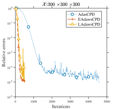
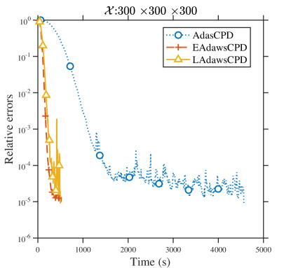
Figure 1: Number of iterations v.s. Relative errors and Time v.s. Relative errors output by the algorithms with $Tol=10^{-5}$, $|\mathcal{F}_{n}|=18$, $R=10$, $noise=0$, and random initialization for the tensor with $I=300$, $R_{true}=10$, $spread=45$, and $magnitude=36$.

In Table 2, we list the performance of algorithms for tensors with different sizes. From this table, we can see that our algorithms have better performance than AdasCPD in fu2020BlockRandomizedStochastic in terms of the number of iterations and overall running time. Some specific discussions of the performance are in order.

1. With the increase of tensor size, EAdawsCPD and LAdawsCPD always have better performance in terms of the iterations and running time compared with AdasCPD.

2. For the probability distribution, the leverage-based algorithm needs a few more iterations than the Euclidean-based algorithm, and the gap is getting larger as the tensor size increases. The reason may be that the latter has a theoretical guarantee that such probability distribution is reasonable needell2017BatchedStochastic ; needell2016StochasticGradient , while the former has no similar theoretical result and is more of an empirical choice.

3. Theoretically, the running time of a single step of our algorithms will be a little more than that of AdasCPD. This is because our algorithms use the importance sampling probability distributions which are a little expensive to compute. However, the importance sampling can improve convergence speed and hence can reduce iterations. So, the overall running time of our algorithms is still much less than that of AdasCPD.

Besides, to make the above comparison more intuitive, we also plot the numerical results for $I=300$ from Table 2 in Figure 1, from which we can see that AdasCPD indeed converges slowly and is unstable. Whereas, our algorithms have quite good performance.

Table 3: Performance of the algorithms with $Tol=10^{-5}$, $|\mathcal{F}_{n}|=18$, different target ranks $R$, $noise=0$, and random initialization for the tensor generated by $300\times 10$ factor matrices with $spread=45$ and $magnitude=36$.

Algorithms		$R=5$	$R=10$	$R=15$	$R=20$
AdasCPD fu2020BlockRandomizedStochastic	Iterations	3059.1	3105.8	4823.7	7094.8
	Seconds	480.47423	472.43042	767.12695	1125.8787
EAdawsCPD	Iterations	474	390.3	406.7	824.9
	Seconds	73.963123	58.656213	65.151505	132.01017
LAdawsCPD	Iterations	535.7	429.9	567.1	827.1
	Seconds	83.791824	64.193687	90.722473	132.73588

In Table 3, we list the performance of algorithms with different target ranks for the same tensor. Numerical results show that our algorithms always perform much better than AdasCPD in iterations and running time. Furthermore, for all the algorithms, the closer the target rank is to the true rank, the better the results are.

To validate the robustness of our algorithms to noises, we run additional experiments on the same synthetic tensor with Gaussian noises with different standard deviations. The results, shown in Table 4, indicate that the earlier experiment results are indeed robust to noises.

Table 4: Performance of the algorithms with $Tol=10^{-5}$, $|\mathcal{F}_{n}|=18$, the target rank $R=10$, and random initialization for different tensors generated by $300\times 10$ factor matrices with $spread=45$, $magnitude=36$, and different noises.

Algorithms		$noise=0$	$noise=0.01$	$noise=0.1$	$noise=1$
AdasCPD fu2020BlockRandomizedStochastic	Iterations	3105.8	3211.7	3024.9	3511.2
	Seconds	472.430421	505.928736	481.988384	553.33599
EAdawsCPD	Iterations	390.3	360.5	381.6	414.6
	Seconds	58.6562125	56.748149	60.5743992	65.3003044
LAdawsCPD	Iterations	429.9	410	439	452.1
	Seconds	64.1936869	64.6965127	70.8384762	71.6683267

In addition, as in fu2020BlockRandomizedStochastic , our algorithms can also be generalized to nonnegative or other constrained situations. So, we also present the comparison of the algorithms with nonnegative constraints in Table 5 and Figure 2, from which we can see that the earlier experiment results are also robust to constraints.

Table 5: Performance of the algorithms with $Tol=10^{-5}$, $|\mathcal{F}_{n}|=18$, the target rank $R=10$, $noise=0$, and random initialization for different tensors generated by $I\times 10$ factor matrices with different $I$ under nonnegative constraint.

Algorithms		$I=100$	$I=200$	$I=300$	$I=400$	$I=500$
		$spread=15$, $magnitude=24$	$spread=30$, $magnitude=30$	$spread=45$, $magnitude=36$	$spread=60$, $magnitude=42$	$spread=75$, $magnitude=48$
AdasCPD fu2020BlockRandomizedStochastic	Iterations	500.1	910.7	1424.5	2203.7	3372.8
	Seconds	2.0256353	28.981344	225.79166	737.83326	2550.5717
EAdawsCPD	Iterations	156.6	190.6	250.6	319	394.2
	Seconds	0.6437757	6.0335162	40.041681	110.00088	299.55425
LAdawsCPD	Iterations	153.7	205.9	271.5	337.5	437.6
	Seconds	0.6892614	6.6271954	43.308729	111.84547	331.55795

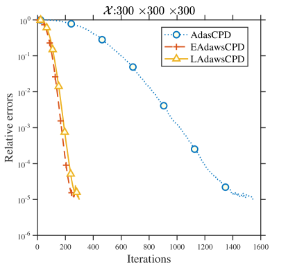
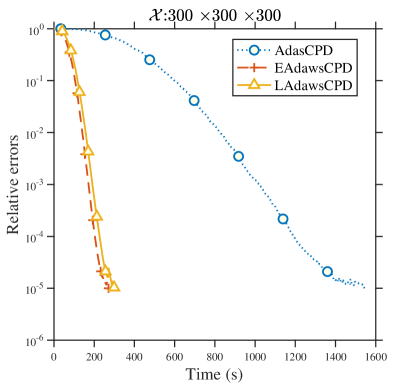
Figure 2: Number of iterations v.s. Relative errors and Time v.s. Relative errors output by the algorithms with $Tol=10^{-5}$, $|\mathcal{F}_{n}|=18$, $R=10$, $noise=0$, and random initialization for the tensor with $I=300$, $R_{true}=10$, $spread=45$, $magnitude=36$, and $\mathbf{A}^{(n)}\geq\bm{0}$.

Finally, using the tensor for Figure 1 (Data I in short), we compare the variances of stochastic gradients listed in Table 1. Meanwhile, we also consider another two tensors: Data II, which is generated by three factor matrices of size $300\times 10$ with independent standard Gaussian entries, and Data III, which is the same as Data II except that one entry of each factor matrices is chosen uniformly and set to 20.

All the numerical results are reported in Figure 3, from which we can see that all the variances decrease with the increase of iterations, and the variances related to importance sampling are not worse than the corresponding ones based on uniform sampling. Moreover, for Data I and Data III, the former is much smaller than the latter, and decrease much faster as the number of iterations increases. This is mainly because the factor matrices for forming the tensors have high coherence, i.e., their maximal leverage scores are large.

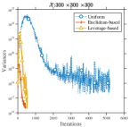
(a) Data I

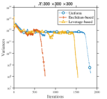
(b) Data II

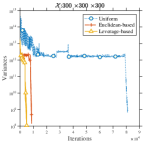
(c) Data III

Figure 3: Comparison of variances of stochastic gradients for different tensors.

5.3 Real data

In this subsection, we test our algorithms on hyperspectral images (HSIs), which are special images with two spatial coordinates and one spectral coordinate. We consider three data tensors available at http://www.ehu.eus/ccwintco/index.php/HyperspectralRemoteSensingScenes. Their brief information is listed in Table 6.

Table 6: Size and type of real datasets.

Dataset	Size	Type
SalinasA.	$83\times 86\times 224$	Hyperspectral
Indian Pines	$145\times 145\times 220$	Hyperspectral
Pavia Uni.	$610\times 340\times 103$	Hyperspectral

Table 7: Performance of algorithms on real datasets.

Algorithms		SalinasA.	Indian Pines	Pavia Uni.
		$R=10$, $|\mathcal{F}_{n}|=20$	$R=10$, $|\mathcal{F}_{n}|=20$	$R=100$, $|\mathcal{F}_{n}|=20$
AdasCPD fu2020BlockRandomizedStochastic	$Tol$	0.00697493	0.00782241	0.02831117
	Seconds	288.535306	653.276364	4387.12147
EAdawsCPD	$Tol$	0.00611473	0.00725646	0.02792415
	Seconds	291.374795	659.02316	4450.21809
LAdawsCPD	$Tol$	0.00644397	0.00741898	0.02796972
	Seconds	295.962095	663.648648	4559.80737

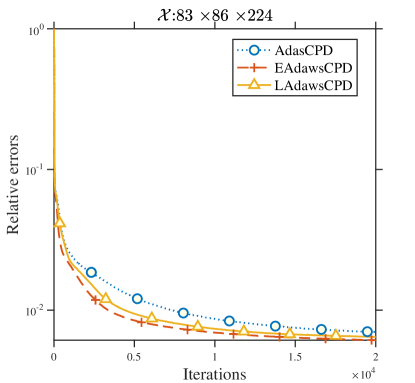
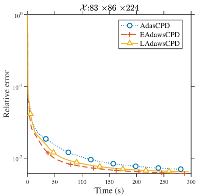
Figure 4: Number of iterations v.s. Relative errors and Time v.s. Relative errors output by the algorithms with $|\mathcal{F}_{n}|=20$ and $R=10$ for SalinasA..

Table 7 shows the relative errors and running time of algorithms for these tensors under different target ranks. The numerical results are returned after 20000 iterations (30000 iterations for Pavia Uni.) with the standard Gaussian matrices being the initial factor matrices. We also plot the results of SalinasA. from Table 7 in Figure 4. It is seen that our algorithms still outperform AdasCPD. However, in contrast to the results for synthetic data, the differences between them are not very remarkable. The main reason may be that these real data are very even. To illustrate, we plot the leverage scores and coherence of the coefficient matrices $\mathbf{Z}^{(n)}$ of CP-ALS subproblems in Figure 5. For comparison, we also plot the corresponding results for Data I mentioned above. Examining the vertical coordinates of Figures 5a, 5b, 5c and 5d attentively, we can observe that the leverage scores for the three real datasets oscillate in a narrower range compared with Data I. Additionally, Figure 5e shows that the coherence of these real data are indeed not very high. In addition, we also plot the squared Euclidean norms of the rows of the coefficient matrices and their maximum values in Figure 6. The findings are similar.

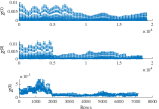
(a) SalinasA.

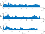
(b) Indian Pines

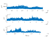
(c) Pivia Uni.

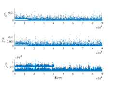
(d) Data I

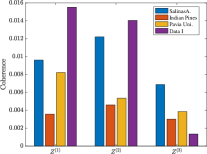
(e) Bar chart

Figure 5: (a)-(d) Leverage scores for four different tensors. (e) Coherence for four different tensors.

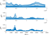
(a) SalinasA.

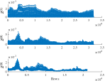
(b) Indian Pines

(c) Pivia Uni.

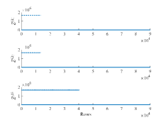
(d) Data I

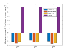
(e) Bar chart

Figure 6: (a)-(d) Squared Euclidean norms for four different tensors. (e) Maximum squared Euclidean norms for four different tensors.

6 Concluding Remarks

In this paper, based on two different sampling strategies, we propose a block-randomized gradient descent method with importance sampling for CP decomposition, and provide its detailed theoretical analysis. Numerical experiments show that our method always outperforms the existing one, AdasCPD. As done in wang2021momentum , it is interesting to consider the momentum version of our method. Also, it is interesting to introduce the greedy sampling strategies bai2018GreedyRandomized ; zhang2022GreedyMotzkin and the scaling technique tong2021AcceleratingIllconditioned into our method. We leave them for future research.

Funding

This work was supported by the National Natural Science Foundation of China (No. 11671060) and the Natural Science Foundation Project of CQ CSTC (No. cstc2019jcyj-msxmX0267).

Data Availability

The data that support the findings of this study are available from the corresponding author upon reasonable request.

Competing Interests

The authors declare that they have no conflict of interest.

References

- \bibcommenthead
- (1) Kolda, T.G., Bader, B.W.: Tensor decompositions and applications. SIAM Rev. 51(3), 455–500 (2009). https://doi.org/10.1137/07070111X
- (2) Sidiropoulos, N.D., De Lathauwer, L., Fu, X., Huang, K., Papalexakis, E.E., Faloutsos, C.: Tensor decomposition for signal processing and machine learning. IEEE Trans. Signal Process. 65(13), 3551–3582 (2017). https://doi.org/10.1109/TSP.2017.2690524
- (3) Carroll, J.D., Chang, J.J.: Analysis of individual differences in multidimensional scaling via an N-way generalization of “Eckart-Young” decomposition. Psychometrika 35(3), 283–319 (1970). https://doi.org/10.1007/BF02310791
- (4) Harshman, R.A.: Foundations of the PARAFAC procedure: Models and conditions for an “explanatory” multimodal factor analysis. UCLA Working Papers in Phonetics 16, 1–84 (1970)
- (5) Battaglino, C., Ballard, G., Kolda, T.G.: A practical randomized CP tensor decomposition. SIAM J. Matrix Anal. Appl. 39(2), 876–901 (2018). https://doi.org/10.1137/17M1112303
- (6) Drineas, P., Mahoney, M.W., Muthukrishnan, S., Sarlós, T.: Faster least squares approximation. Numer. Math. 117(2), 219–249 (2011). https://doi.org/10.1007/s00211-010-0331-6
- (7) Fu, X., Ibrahim, S., Wai, H.T., Gao, C., Huang, K.: Block-randomized stochastic proximal gradient for low-rank tensor factorization. IEEE Trans. Signal Process. 68, 2170–2185 (2020). https://doi.org/10.1109/TSP.2020.2982321.
- (8) Wang, Q., Cui, C., Han, D.: A momentum block-randomized stochastic algorithm for low-rank tensor CP decomposition. Pac. J. Optim. 17(3), 433–452 (2021)
- (9) Larsen, B.W., Kolda, T.G.: Practical Leverage-Based Sampling for Low-Rank Tensor Decomposition. arXiv:2006.16438 (2020)
- (10) Cheng, D., Peng, R., Perros, I., Liu, Y.: SPALS: Fast alternating least squares via implicit leverage scores sampling. In: Proceedings of the 30th International Conference on Neural Information Processing Systems, pp. 721–729. Curran Associates Inc., Barcelona Spain (2016)
- (11) Vervliet, N., Debals, O., Sorber, L., De Lathauwer, L.: Breaking the curse of dimensionality using decompositions of incomplete tensors: Tensor-based scientific computing in big data analysis. IEEE Signal Process. Mag. 31(5), 71–79 (2014). https://doi.org/10.1109/MSP.2014.2329429
- (12) Bhojanapalli, S., Sanghavi, S.: A new sampling technique for tensors. In: Proceedings of the 30th International Conference on Neural Information Processing Systems, pp. 3008–3016. Curran Associates Inc., Barcelona Spain (2016)
- (13) Vu, X.T., Maire, S., Chaux, C., Thirion-Moreau, N.: A new stochastic optimization algorithm to decompose large nonnegative tensors. IEEE Signal Process. Lett. 22(10), 1713–1717 (2015). https://doi.org/10.1109/LSP.2015.2427456
- (14) Beutel, A., Talukdar, P.P., Kumar, A., Faloutsos, C., Papalexakis, E.E., Xing, E.P.: FlexiFaCT: Scalable flexible factorization of coupled tensors on hadoop. In: Proceedings of the 2014 SIAM International Conference on Data Mining (SDM), pp. 109–117. SIAM, Philadelphia, PA. (2014)
- (15) Vervliet, N., De Lathauwer, L.: A randomized block sampling approach to Canonical Polyadic decomposition of large-scale tensors. IEEE J. Sel. Topics Signal Process. 10(2), 284–295 (2016). https://doi.org/10.1109/JSTSP.2015.2503260
- (16) Needell, D., Srebro, N., Ward, R.: Stochastic gradient descent, weighted sampling, and the randomized Kaczmarz algorithm. Math. Program. 155(1), 549–573 (2016). https://doi.org/10.1007/s10107-015-0864-7
- (17) Drineas, P., Magdon-Ismail, M., Mahoney, M.W., Woodruff, D.P.: Fast approximation of matrix coherence and statistical leverage. J. Mach. Learn. Res. 13(1), 3475–3506 (2012)
- (18) Woodruff, D.P.: Sketching as a tool for numerical linear algebra. Found. Trends Theor. Comput. Sci. 10(1–2), 1–157 (2014). https://doi.org/10.1561/0400000060
- (19) Xu, Y., Yin, W.: A block coordinate descent method for regularized multiconvex optimization with applications to nonnegative tensor factorization and completion. SIAM J. Imaging Sci. 6(3), 1758–1789 (2013). https://doi.org/10.1137/120887795
- (20) Ma, P., Mahoney, M., Yu, B.: A statistical perspective on algorithmic leveraging. J. Mach. Learn. Res. 16(27), 861–911 (2015)
- (21) Bader, B.W., Kolda, T.G., et al.: Tensor Toolbox for MATLAB. Version 3.2.1 (2021). https://www.tensortoolbox.org Accessed 2021/04/05
- (22) Needell, D., Ward, R.: Batched stochastic gradient descent with weighted sampling. In: Approximation Theory XV: San Antonio 2016, vol. 201, pp. 279–306. Springer, Cham (2017)
- (23) Bai, Z.Z., Wu, W.T.: On greedy randomized Kaczmarz method for solving large sparse linear systems. SIAM J. Sci. Comput. 40(1), 592–606 (2018). https://doi.org/10.1137/17M1137747
- (24) Zhang, Y.J., Li, H.Y.: Greedy Motzkin-Kaczmarz methods for solving linear systems. Numer. Linear Algebra Appl. 29(2), 2429 (2022). https://doi.org/10.1002/nla.2429
- (25) Tong, T., Ma, C., Chi, Y.: Accelerating ill-conditioned low-rank matrix estimation via scaled gradient descent. J. Mach. Learn. Res. 22(150), 1–63 (2021)