Long characteristics vs. short characteristics
in 3D radiative transfer simulations of polarized radiation

Abstract

We compare maps of scattering polarization signals obtained from three-dimensional (3D) radiation transfer calculations in a magneto-convection model of the solar atmosphere using formal solvers based on the “short characteristics” (SC) and the “long characteristics” (LC) methods. The SC method requires less computational work, but it is known to introduce spatial blurring in the emergent radiation for inclined lines of sight. For polarized radiation this effect is generally more severe due to it being a signed quantity and to the sensitivity of the scattering polarization to the model’s inhomogeneities. We study the differences in the polarization signals of the emergent spectral line radiation calculated with such formal solvers. We take as a case study already published results of the scattering polarization in the Sr I 4607 Å line obtained with the SC method, demonstrating that in high-resolution grids it is accurate enough for that type of study. In general, the LC method is the preferred one for accurate calculations of the emergent radiation, reason why it is now one of the options in the public version of the 3D radiative transfer code PORTA.

1 Introduction

The modeling of the scattering polarization in spectral lines using three-dimensional (3D) models of stellar atmospheres requires the solution of the radiative transfer problem without assuming local thermodynamic equilibrium. The statistical equilibrium equations (SEE) and the radiation transfer equations (RTE) must be solved iteratively, as both sets of equations are coupled and the problem as a whole is non-linear and non-local.

In practice, the solution of the RTE is the most computationally demanding part. Nowadays, the RTE are usually solved via the short characteristics (SC) method (for a review of the methods used prior to the SC method see, e.g., Jones 1973; Jones & Skumanich 1973; Crosbie & Linsenbardt 1978). Kunasz & Auer (1988) developed the SC method based on the parabolic approximation of the source function. Different approximations of the source function that avoid the introduction of new local extrema were later introduced, such as piecewise cubic Hermite interpolation and monotonic Bezier splines (Auer 2003; Štěpán & Trujillo Bueno 2013; de la Cruz Rodríguez & Piskunov 2013).

The main advantage of the SC method is its efficiency, as it scales with just the number of grid points. However, this method is known to introduce diffusion (Kunasz & Auer 1988; Leenaarts 2020). While in practice this diffusion is not a problem regarding the calculation of the mean radiation field within the 3D model, this is not necessarily the case when calculating the linear polarization caused by the scattering of anisotropic radiation. Not only is the polarization a signed quantity (thus prone to signal cancellation), but it depends dramatically on the geometry and the spatial variation of the plasma properties (e.g., Manso Sainz & Trujillo Bueno 2011).

In this paper we study the effect of the diffusion in the SC method in the formal solution to compute the emergent Stokes profiles in a 3D model of the solar atmosphere. In §2 we briefly describe the SC and long characteristics (LC) methods and we give some details on the implementation of such methods in the radiation transfer code PORTA. The comparison of the results with the two methods is shown in §3. Finally, we present our conclusions in §4.

2 The SC and LC methods

The RTE for the Stokes-$I$ parameter, which describes the propagation of the intensity of a radiation beam through a medium for a given frequency and direction, can be written as (e.g., Mihalas et al. 1978)

$$\frac{dI}{ds}=-\eta_{I}I+\epsilon_{I},$$ (1)

where $I$ is the intensity Stokes parameter, $\eta_{I}$ is the extinction coefficient and $\epsilon_{I}$ is the emissivity. Introducing the optical depth $d\tau=-\eta_{I}ds$, the intensity of the beam of radiation of a given frequency after travelling through a medium an optical depth $\Delta\tau$ in a given propagation direction is

$$I(\Delta\tau)=I(0)e^{-\Delta\tau}+\int^{\Delta\tau}_{0}Se^{-t}dt,$$ (2)

where $I(0)$ is the intensity at the beginning of the propagation path and $S=\epsilon_{I}/\eta_{I}$ is the source function. Equations (1)-(2) are easily generalized to the equations for the four Stokes parameters $I$, $Q$, $U$, and $V$ we actually use (see Landi Degl’Innocenti & Landolfi 2004). However, the intensity only equations are enough for the purpose of this section.

The “characteristics” methods solve Eq. (2) by assuming a functional form for the source function $S$. However, the SC and LC methods differ on whether we use short or long characteristics for each ray direction, as explained below.

In the SC method, for every point of the grid we take the closest intersections between the propagating beam and the surfaces between the surrounding grid points, both forward and backward along the propagation direction. Because, in general, only the central point under consideration corresponds exactly with a grid point, all quantities in Eq. (2) ($\eta_{I}$, $\epsilon_{I}$, and $I(0)$) must be interpolated from the surrounding grid points into the intersections (Kunasz & Auer, 1988).

As for the LC method, for every point of the grid the beam is propagated backwards until the boundary of the computational domain is reached. Then, Eq. (2) is sequentially solved along the ray. Generally, as in the SC method, only the point under consideration coincides with a grid point and, therefore, interpolation is necessary. However, while both SC and LC require the interpolation of the radiation transfer coefficients $\eta_{I}$ and $\epsilon_{I}$ at every surface between the model’s grid points, the LC method only requires the interpolation of $I(0)$ at the boundary of the domain.

Given a cubic domain of side $N$, the computational work of the SC method scales as $N{}^{3}$, while that of the LC method scales as $N{}^{4}$. The SC method is significantly computationally less expensive than the LC one, but in coarse grids it introduces numerical diffusion due to the high number of upwind interpolations of the intensity needed. This is even more acute when the propagation direction has a large angle from the vertical, in which case it cuts vertical planes, for which further interpolations of the intensity ($I(0)$ in Eq. (2)) are needed, which in turn increase the diffusion. In Fig. 1 we show the interpolations required in order to calculate the intensity at a given grid point $\mathbf{P}$ for propagation directions with a small (left panel) and a large (right panel) angle with respect to the vertical, assuming periodic horizontal boundary conditions. The “Int” labels in the figure indicate where it is necessary to interpolate the incoming intensity ($I(0)$ in Eq. (2)), and the dotted curves indicate the points needed for the interpolation (assuming linear order interpolations). For propagation directions close to the vertical, calculating the intensity at grid point $\mathbf{P}$ requires the intensity at point $a$ in the figure, which needs to be interpolated from the values at the grid points $b$ and $c$. These points, in turn, need the intensity values from the horizontal plane immediately below, which also need to be interpolated from their closest grid points. This procedure is propagated backwards until we reach the bottom plane, where the given boundary condition is used in the interpolations. Therefore, the calculation of the intensity at point $\mathbf{P}$ as depicted in Fig. 1 would require six interpolations. Likewise, for a significantly inclined propagation direction, the calculation of the intensity at grid point $\mathbf{P}$ requires the intensity at point $a$ in the figure, and this value needs to be interpolated from the intensity values at the $b$ and $c$ grid points. The procedure is analogous to the previous case until we reach the left vertical boundary plane. Points $d$, $e$, and $f$ in the figure cannot be interpolated from boundary condition values. Instead, these rays propagate cycling through the domain (dashed lines in the figure). At the next intersection with a vertical or horizontal plane (as in the figure), further interpolations are required. Thus, the calculation of the intensity for the large angle case at point $\mathbf{P}$ as depicted in the figure would require nine interpolations.

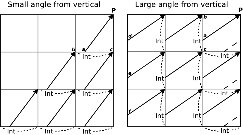
Figure 1: Diffusion increases for large angles from the vertical with the SC method. The “Int” labels in the figure indicate where it is necessary to interpolate the intensity ($I(0)$ in Eq. (2)). See full explanation in main text.

Fig. 2 shows the difference between the SC and LC methods in 2D. With the SC method (left panel), we need to interpolate the intensity values for each short ray. With the LC method (right panel), we only need to interpolate the intensity values in the bottom boundary, which are then propagated through the domain (as in Fig. 1 the dashed lines represent the continuation of rays that leave the left boundary).

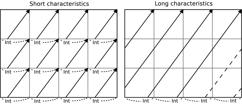
Figure 2: Propagation strategy to compute the radiation emerging at the top plane with the SC and the LC methods. The “Int” labels in the figure indicate where it is necessary to interpolate the intensity ($I(0)$ in Eq. (2)). The interpretation of the dotted curves and the dashed lines are as per Fig. 1.

Depending on the particular sampling of the model and the inclination of the propagation rays, the difference between the solution calculated with SC and LC can be quite substantial, as we will show in following sections.

2.1 PORTA

PORTA is a 3D radiation transfer code capable of calculating the intensity and polarization of the emergent radiation taking into account scattering processes and the Hanle and Zeeman effects (Štěpán & Trujillo Bueno 2013, publicly available at https://gitlab.com/polmag/PORTA).

This numerical code solves the radiation transfer problem iteratively with the Jacobi method. In order to compute the radiation field at every point, frequency, and direction within the atmospheric model, PORTA solves the RTE with the SC method. Once the self-consistent solution has been achieved, we can obtain the emergent Stokes profiles at every point of the model’s surface for the desired line of sight (LOS) with a single formal solution , which can be efficiently performed with either the SC or the LC method. The computing time penalty incurred by using the LC instead of the SC method for a single formal solution is larger as the inclination $\theta$ with respect to the vertical increases, but never by more than $\sim 58$% for the performed tests (see Fig. 3, for the 3D model described in §3). Note that the LC method is never used in PORTA when looking for the self-consistent solution because this would require, for every iterative step, to compute the radiation field not only at the model’s surface, but for all grid points, which would make the computing time required for solving the problem completely prohibitive.

Previous results using the PORTA code, such as those by del Pino Alemán et al. (2018), made use of the SC method to compute the emergent Stokes profiles. Recently, the LC method for the formal solution was implemented in the public version of PORTA, making it possible to test the accuracy of the results obtained using the faster SC method.

Figure 3: Computing time required with the PORTA code for one formal solution of the Stokes parameters in the Sr I 4607 Å line in model atmospheres with four different horizontal spatial resolutions, ranging from 16 km to 128 km, and constant vertical resolution of 16 km. The time difference is small for small inclinations $\theta$ with respect to the vertical and increases with it. For (a) $\theta=0$ the maximum relative difference between computing times is $\sim 11$%, while for (b) $\theta=80$ it is $\sim 58$%.

2.2 3D Test of a Beam Propagating in Vacuum

One of the simplest tests to demonstrate the numerical dispersion of the radiation is the propagation of a single beam in vacuum (Auer et al. 1994). We have performed this test with both the SC and LC methods using several grids with different box sizes and resolutions. The extinction and source functions are set to zero everywhere (vacuum), as well as the incoming radiation in the boundaries, except for a single point in the centre of the bottom boundary, and only in one propagation direction.

When the propagation direction is along the vertical, all points along the characteristics correspond to nodes in the model. Therefore, there is no dispersion and SC and LC are equivalent. However, when the propagation direction is not parallel to any of the axis of the Cartesian grid, interpolations are needed.

Fig. 4 shows the case of a propagation direction inclined $60^{\circ}$ from the vertical, using a domain size of $\sim 1.5\times 1.5\times 1$ Mm³. Even when the grid has very high resolution ($8$ km), the dispersion in the calculation with SC is evident (see top row in the figure). This dispersion is stronger when the length of the propagation path increases and when the grid resolution decreases (see bottom row in the figure for the $16$ km and $32$ km resolution grids).

Figure 4: Propagation of a beam of radiation in vacuum along a direction inclined $60^{\circ}$ from the vertical axis in a Cartesian grid computed with: (a) LC; (b), (c) and (d) SC. The domain is $\sim 1.5\times 1.5\times 1$ Mm³ in all panels. The LC solutions are virtually identical for all grid resolutions, since the only intensity interpolation happens at the bottom boundary, so we only show the case for resolution of $8\times 8\times 8$ km (a). In the case of SC, the dispersion is different depending on the grid resolution and inclination of the beam, and we present three cases: $8\times 8\times 8$ km (b), $16\times 16\times 16$ km (c) and $32\times 32\times 32$ km (d), all saturated at 25% of the original beam intensity for ease of comparison.

We have also performed this test with the same grid as the one used in del Pino Alemán et al. (2018) (a $\sim 6\times 6\times 1$ Mm³ box with $8$ km resolution in the three dimensions), and Fig. 5 shows the emergent intensity at the top boundary of the corresponding vacuum box. It is clear from this figure that the emergent Stokes parameters will suffer from “smearing” effects whenever SC is used to compute the formal solution, while the LC algorithm prevents such effects.

Figure 5: Emergent intensity at the top boundary for a beam of radiation of $I=1$ in vacuum propagating in a direction inclined $20^{\circ}$ from the vertical axis in a Cartesian grid of $8\times 8\times 8$ km resolution using (a) SC and (b) LC.

3 Comparing the LC and SC results

We take as a test case the Sr I 4607 Å line investigation by del Pino Alemán et al. (2018) where the SC formal solver was used both in the iterative solution and in the calculation of the Stokes profiles of the emergent radiation after obtaining the self-consistent solution of the radiation transfer problem. To confront the LC and SC methods, we compare the ensuing scattering polarization signals of the emergent spectral line radiation calculated in a 3D magneto-hydrodynamical model of the quiet solar photosphere by Rempel (2014). The model is characterized by a mean field strength $\langle B\rangle\approx 170$ G at the model’s visible surface, with a physical size of $\sim 6\times 6\times 1$ Mm³ (in a grid of $768\times 768\times 137$ points and $8$ km of spatial resolution). Further details about this model of the solar photosphere can be found in Rempel (2014) and del Pino Alemán et al. (2018). Starting from the self-consistent solution calculated by del Pino Alemán et al. (2018) in the 3D model of Rempel (2014), we calculate the emergent Stokes parameters using the LC formal solver. We then compare these results with the ones shown in del Pino Alemán et al. (2018), computed using the SC formal solver. We used a two-level atomic model with the Sr I ground level ¹S₀ and the line’s upper level ¹P₁, whose angular momentum values are $J_{l}=0$ and $J_{u}=1$, respectively, and with total number densities calculated with a more complex model atom (see del Pino Alemán et al. (2018) for details).

3.1 Impact on the center-to-limb variation (CLV)

First, we study the impact on the center-to-limb variation (CLV) of the linear polarization (Fig. 12 in del Pino Alemán et al., 2018). Because the calculated CLV lacks spatial resolution (that is, for every line of sight the whole field of view was integrated), the effects of the dispersion should be attenuated. This is exactly what is found in Fig. 6, which shows the CLV of the fractional linear polarization $Q/I$ computed in the $8$ km grid using the SC and LC methods in the formal solver. For both Figs. 6 and 7, we considered twenty equally spaced $\mu$ values in the range [0.2,0.6] and, for each of them, twelve equally spaced azimuths. The differences between the two calculations are visible at plot level. However, they are small enough so as to be irrelevant in the analysis, as the variations due to the inhomogoneities of the solar atmosphere and the errors of the observational data are larger than the difference in the results obtained with such two formal solution methods.

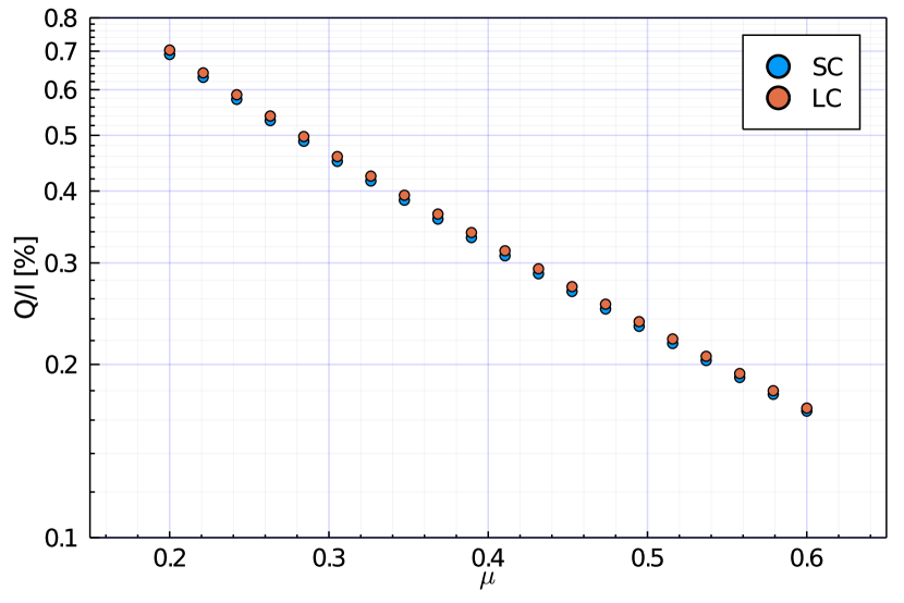
Figure 6: The CLV of the $Q/I$ fractional polarization amplitude calculated in the $8$ km grid after spatially averaging the Stokes $I$ and $Q$ signals, using the SC method (blue dots) and the LC method (orange dots). Each data point in the figure was obtained by integrating over twelve equally spaced azimuths and over the whole field of view corresponding to each line of sight characterized by $\mu$.

It is of interest, however, to find out if this good agreement between the CLV calculated with the two methods is due to the high resolution of the model atmosphere. To this end, we degrade the model by decreasing the resolution of the vertical direction to $16$ km, and the resolution in the horizontal directions to $16$, $32$, $64$, and $128$ km. This degradation was performed by resampling the model, taking every second point when going from $8$ to $16$ km resolution, and again (but only in the horizontal dimensions) from $16$ to $32$ km, from $32$ to $64$ km, and from $64$ to $128$ km resolutions. Interestingly, while the comparison indicates that the worst resolution leads to larger differences between the SC and LC results, they do not show a clear tendency when the resolution is deteriorated (see Fig. 7). We can thus conclude that the CLV of the spatially integrated Stokes parameters is not strongly affected by the dispersion effect of the SC algorithm.

Figure 7: The CLV of the spatially integrated fractional linear polarization $Q/I$ obtained with the SC method (blue dots) and the LC method (orange dots) with a vertical axis resolution of $16$ km and a horizontal axis resolution of (a) $16$, (b) $32$, (c) $64$, and (d) $128$ km. Each data point in the figure was obtained by integrating over twelve equally spaced azimuths and over the whole field of view corresponding to each line of sight characterized by $\mu$.

3.2 Impact on the spatially resolved polarization maps

Secondly, we study the impact on the fractional total linear polarization maps for an inclined LOS. In particular, we choose a LOS with $\mu=0.5$, with $\mu$ the cosine of the heliocentric angle (see the panels of the middle column in Fig. 9 of del Pino Alemán et al. 2018, which they obtained with the SC formal solver in the $8$ km resolution model).

Fig. 8 shows (top panels) the fractional total linear polarization ($\sqrt{Q^{2}+U^{2}}/I$) and the continuum intensity amplitude (bottom panels) maps obtained with the SC and the LC formal solvers. When using the LC solver (right panels), the very fine and detailed structures produced by the model atmosphere are fully preserved. However, when using the SC method (left panels) the numerical dispersion introduces a clear “smearing” effect in the resulting polarization maps.

While this test indicates that, visually, the polarization of the emergent radiation is sensitive to the the formal solver chosen, a more quantitative study is necessary, which is addressed in the following section.

Figure 8: Fractional total linear polarization amplitude (top panels) and continuum intensity amplitude (bottom panels) of the Sr I 4607 Å line calculated for a LOS with $\mu=0.5$ in the full resolution ($8$ km) 3D model using the SC (panels a and c) and LC (panels b and d) formal solvers. Note that the $X$ coordinate in the figure represents the projected $X$ for the $\mu=0.5$ LOS, and not that of the original model.

3.3 Impact on the statistics

Finally, we compare the impact on the scatter plots of linear polarization vs continuum intensity after calculating the emergent Stokes profiles of the Sr I 4607 Å line. To this end, we have selected the largest signals of the $Q/I$ and $U/I$ profiles of the emergent spectral line radiation for each spatial point of the disk-center field of view, and represented them against the scaled value of the continuum intensity at the same point (see the top panels of the Fig. 18 of del Pino Alemán et al. 2018).

Fig. 9 shows these scatter plots for the original resolution ($8$ km) of the atmospheric model and $\mu=0.5$. While the selection of algorithm for the formal solver does not impact the behaviour (the structure) of the distribution of the points, there are some differences. First, “trails” are more frequent with SC. These trails seem to appear as a consequence of the foreshortening of one of the dimensions for inclined LOS. Along the shortened direction, nodes are closer to each other in the field of view and, therefore, the change of values between nodes is larger in one dimension than in the other, giving rise to the “trails” in the scatter plots.

Secondly, the maximum values of the polarization are larger with LC. This is a consequence of the smearing effect due to the dispersion introduced by the SC algorithm, which smudges the regions with those maximums and decreases its amplitudes.

Figure 9: $Q/I$ (top panels) and $U/I$ (bottom panels) amplitudes of the emergent radiation against the scaled value of the continuum intensity calculated with the SC (panels a and c) and LC (panels b and d) formal solvers. The line of sights have $\mu=0.5$ and eight equally spaced azimuths. The resolution of the model’s grid is $8$ km.

In Fig. 10 we can see the case with horizontal resolution of $128$ km and vertical resolution of $16$ km. For this resolution we see that the differences are larger than in the $8$ km resolution case, changing not only the maximum signals but also altering the shape of the distribution of points. In the low resolution case the maximum values of the polarization signals are larger with LC, and the SC results do not show so clearly the inverse relation between the polarization amplitude and the continuum intensity that del Pino Alemán et al. 2018 found in their $8$ km resolution calculations.

Figure 10: $Q/I$ (top panels) and $U/I$ (bottom panels) amplitudes of the emergent radiation against the scaled value of the continuum intensity calculated with the SC (panels a and c) and LC (panels b and d) formal solvers. The line of sights have $\mu=0.5$ and eight equally spaced azimuths. The resolution of the grid is $128$ km along the horizontal directions and $16$ km along the vertical.

Regarding the total linear polarization (see Fig. 10 of del Pino Alemán et al. 2018), Fig. 11 shows such scatter plots in the full resolution ($8$ km) 3D model applying the SC (top panels) and LC (bottom panels) formal solvers. Three lines of sight with $\mu=0.1$ (left panels), $\mu=0.5$ (middle panels), and $\mu=1$ (right panels) are shown. Similarly to what we observe in Fig. 9, the main difference between the SC (top panels) and LC (bottom panels) solutions is a slight reduction of the maximum polarization values in the SC solution, but the anti-correlation between the total linear polarization amplitude and the continuum intensity pointed out by del Pino Alemán et al. (2018) is confirmed by the LC results. Obviously, the results for $\mu=1$ are identical because, as explained in section §2.2, when the propagation direction is along the vertical all points along the characteristics correspond to nodes and thus there is neither dispersion nor differences between the SC and LC solutions.

Figure 11: Fractional total linear polarization $P$ (at the wavelength where $P$ is maximum) against the scaled value of the continuum intensity calculated with the SC (top panels) and LC (bottom panels) formal solvers. The line of sights have $\mu=0.1$ (left panels), $\mu=0.5$ (middle panels) and $\mu=1$ (right panels). Eight equally spaced azimuths were taken for the $\mu=0.1$ and $\mu=0.5$ cases. The resolution of the model’s grid is $8$ km.

In Fig. 12 we show the case with horizontal resolution of $128$ km and vertical resolution of $16$ km. For this resolution we can see, similarly to Fig. 10, that the differences are larger than in the $8$ km resolution case. The maximum values of the polarization are larger with LC, except for $\mu=1$, which are identical in both solutions (see explanation above).

Figure 12: Fractional total linear polarization $P$ (at the wavelength where $P$ is maximum) against the scaled value of the continuum intensity calculated with the SC (top panels) and LC (bottom panels) formal solvers. The line of sights have $\mu=0.1$ (left panels), $\mu=0.5$ (middle panels) and $\mu=1$ (right panels). Eight equally spaced azimuths were taken for the $\mu=0.1$ and $\mu=0.5$ cases. The resolution of the grid is $128$ km along the horizontal directions and $16$ km along the vertical.

4 Conclusions

Although in 3D models of the solar atmosphere it is unfeasible (due to its scaling) to solve the full iterative problem of scattering line polarization using the LC instead of the SC method, the computational cost increase for a single formal solution is not that significant. We have thus implemented the LC formal solution method for the calculation of the emergent Stokes parameters in the public radiative transfer code PORTA. Starting from the self-consistent solution for the atomic excitation in the Sr I 4607 Å line calculated by del Pino Alemán et al. (2018) in a realistic 3D magneto-convection model, we have computed and compared the emergent Stokes profiles of this spectral line using both the SC and LC algorithms.

When comparing polarization quantities without spatial resolution, such as the CLV, we have found that, as expected, there is little to no impact on the selection of formal solvers, because the lack of spatial resolution conceals the smearing effect of the SC method.

The impact is however noticeable when comparing both results at full spatial resolution. The LC preserves the fine structure of the polarization maps produced by the inhomogeneities in the 3D model atmosphere, and it generally yields larger polarization signals. In contrast, the SC method damps and smears the polarization signals of the emergent spectral line radiation, because of the numerical diffusion inherent to this method.

A comparison of the statistics (scatterplots of polarization against the continuum intensity) also reveals that the main difference between the SC and LC solutions, at the original resolution of the model, is just a slight reduction of the maximum values of the scattering polarization signals, keeping the overall shape of the distribution unchanged. However, the differences increase when the spatial resolution of the model is deteriorated, changing not only the maximum signals but also altering the shape of the distribution of points.

We can thus conclude that, due to the high resolution of the 3D model atmosphere used in del Pino Alemán et al. (2018), the results shown in that paper regarding the comparison with the observed CLV or the statistical relation between polarization signals and continuum intensities are not affected by the use of the SC method. Nevertheless, we recommend the use of the LC formal solver to compute the emergent Stokes profiles, avoiding the smearing effect intrinsic to the SC method without a significant increase on computational cost.

References

- Auer (2003) Auer, L. 2003, in Astronomical Society of the Pacific Conference Series, Vol. 288, Stellar Atmosphere Modeling, ed. I. Hubeny, D. Mihalas, & K. Werner, 3
- Auer et al. (1994) Auer, L., Fabiani Bendicho, P., & Trujillo Bueno, J. 1994, A&A, 292, 599
- Crosbie & Linsenbardt (1978) Crosbie, A. L., & Linsenbardt, T. L. 1978, J. Quant. Spec. Radiat. Transf., 19, 257, doi: 10.1016/0022-4073(78)90061-4
- de la Cruz Rodríguez & Piskunov (2013) de la Cruz Rodríguez, J., & Piskunov, N. 2013, ApJ, 764, 33, doi: 10.1088/0004-637X/764/1/33
- del Pino Alemán et al. (2018) del Pino Alemán, T., Trujillo Bueno, J., Štěpán, J., & Shchukina, N. 2018, ApJ, 863, 164, doi: 10.3847/1538-4357/aaceab
- Jones (1973) Jones, H. P. 1973, ApJ, 185, 183, doi: 10.1086/152407
- Jones & Skumanich (1973) Jones, H. P., & Skumanich, A. 1973, ApJ, 185, 167, doi: 10.1086/152406
- Kunasz & Auer (1988) Kunasz, P., & Auer, L. H. 1988, J. Quant. Spec. Radiat. Transf., 39, 67, doi: 10.1016/0022-4073(88)90021-0
- Landi Degl’Innocenti & Landolfi (2004) Landi Degl’Innocenti, E., & Landolfi, M. 2004, Polarization in Spectral Lines (Kluwer Academic Publishers)
- Leenaarts (2020) Leenaarts, J. 2020, Living Reviews in Solar Physics, 17, 3, doi: 10.1007/s41116-020-0024-x
- Manso Sainz & Trujillo Bueno (2011) Manso Sainz, R., & Trujillo Bueno, J. 2011, ApJ, 743, 12, doi: 10.1088/0004-637X/743/1/12
- Mihalas et al. (1978) Mihalas, D., Auer, L. H., & Mihalas, B. R. 1978, ApJ, 220, 1001, doi: 10.1086/155988
- Rempel (2014) Rempel, M. 2014, ApJ, 789, 132, doi: 10.1088/0004-637X/789/2/132
- Štěpán & Trujillo Bueno (2013) Štěpán, J., & Trujillo Bueno, J. 2013, A&A, 557, A143, doi: 10.1051/0004-6361/201321742