Simplicial Complex Representation Learning

Abstract

Simplicial complexes form an important class of topological spaces that are frequently used in many application areas such as computer-aided design, computer graphics, and simulation. Representation learning on graphs, which are just 1-d simplicial complexes, has witnessed a great attention in recent years. However, there has not been enough effort to extend representation learning to higher dimensional simplicial objects due to the additional complexity these objects hold, especially when it comes to entire-simplicial complex representation learning. In this work, we propose a method for simplicial complex-level representation learning that embeds a simplicial complex to a universal embedding space in a way that complex-to-complex proximity is preserved. Our method uses our novel geometric message passing schemes to learn an entire simplicial complex representation in an end-to-end fashion. We demonstrate the proposed model on a publicly available mesh dataset. To the best of our knowledge, this work presents the first method for learning simplicial complex-level representations.

1 Introduction

Object representation learning aims to learn a mapping that embeds the elementary components of this object into some Euclidean space while preserving the object’s structural information. Recently, such methods have gained a great momentum especially with graph representation learning. The latter has attracted considerable popularity over the past few years with success in both node-level representation learning Cui et al. (2018) and entire graph learning Narayanan et al. (2017); Tsitsulin et al. (2018). The applications of such representation on graphs are diverse as they can be used for almost any downstream machine learning task on domains such as graph classification Hamilton et al. (2017a) or similarity Heimann et al. (2018).

Despite the success of graph representation learning in the past few years, there is a gamut of applications, e.g. in neuroscience Tang et al. (2019); Nasrin et al. (2019); Maroulas et al. (2019); Oballe et al. (2021) where learning in cliques of nodes and how the information passes among these cliques are urgently required, there has not been enough efforts to extend representation learning to simplicial complexes. In general, topological considerations of the underlying data and their relationships encapsulate rich information which one may harness, e.g. see Love et al. (2021); Maroulas et al. (2021). The higher dimensional simplicial complexes often hold additional structure over graphs that might be critical in modeling and must be incorporated to learn the correct representation. For instance, when a simplicial complex is a triangulated manifold, then the aim is to design an algorithm that uncovers the manifold in the learnt representation. Motivated by the success of graph representation learning, we propose a method for learning simplicial complex representation. Our method utilizes a complex autoencoder proposed in Hajij et al. (2020a) and learns an entire simplicial complex representation extracted from simplices embeddings vectors induced by the simplicial complex autoencoder. Our learning function maps every simplicial complex to a universal embedding space in a way that complex-to-complex proximity is preserved. Learning simplicial complex-level representation is essential to perform downstream machine learning tasks on these objects such as simplicial complex classification and similarity ranking. See for instance Hajij et al. (2018); Fey & Lenssen (2019); Ying et al. (2018); Narayanan et al. (2017) for related studies on graphs.

The literature of entire graph representation learning is rich and many methods have been proposed including Laplacian-based methods de Lara & Pineau (2018); Tsitsulin et al. (2018), implicit factorization techniques Chen & Koga (2019); Narayanan et al. (2017), GNN-based methods Bai et al. (2019), and pooling based methods Ying et al. (2018). We refer the reader to Cui et al. (2018) for a recent survey on network embedding. In addition, simplicial complex representation learning, inspired by the success of node2vec Angles & Gutierrez (2008) and Word2Vec Mikolov et al. (2013), started to get attention recently. For example, the works in Billings et al. (2019); Schaub et al. (2020) define simplicies emebddings based random walks on simplicial complexes. This was generalized to $k$-simplex embeddings in Hacker (2020). A general cell complex autoencoder scheme that describes these random walk-based representations as special cases was suggested in Hajij et al. (2020a).

Although there are several methods for learning simplex-level representation Billings et al. (2019); Schaub et al. (2020); Hajij et al. (2020a); Hacker (2020), the work herein is the first to propose a learning representation of the entire simplicial complex. Further, we show our simplicial complex autoencoder (SCA) on a publicly available mesh dataset and demonstrate promising preliminary results. The rest of the paper is organized as follows. Notation and necessary definitions on simplicial complexes are given in Section 2. Section 3 is devoted to reviewing cell complex neural networks. Our proposed simplicial complex autoencoder (SCA) is given in Section 4.1. Finally, Section 5 shows the results.

2 Simplicial Complex Neighborhood Matrices

This section provides the necessary notations to define neighborhood matrices between simplices in a simplicial complex, and hence, we assume the reader has familiarity with basic definitions of simplicial complexes Hatcher (2005). Let $X$ be a simplicial complex and $n$ be the dimension of $X$. Recall that the dimension of $X$ is the dimension of the highest simplex in $X$. For any $0\leq k\leq n$, we denote the set of all $k$-simplices in $X$ by $X^{k}$. If $X$ is a simplicial complex of dimension $n$, then for every $0<m\leq n$ we denote the set of simplicies in $X$ with dimension less than $m$ by $X^{<m}$. The set $X^{>m}$ is defined similarly. In this work, we assume that the complex $X$ is unoriented. However, the following notion of neighbored on simplicial complexes can be easily extended to oriented simplicial complexes; see for instance Hajij et al. (2020a); Glaze et al. (2021) for various considerations on oriented simplical complexes in the context of neural network computations.

Adjacency relations can be defined on simplicial complexes in a similar fashion as they are defined on graphs. Specifically, let $X$ be a simplicial complex and let $c^{n}$ denotes a $n$-simplex in $X$, and $facets(c^{n})$ denotes the set of all $(n-1)$-simplicies $X$ incident to $c^{n}$. Two $n$-simplices $a^{n}$ and $b^{n}$ are said to be adjacent if there exists an $(n+1)$-simplex $c^{n+1}$ such that $a^{n},b^{n}\in facets(c^{n+1})$. The set of all simplices adjacent to a simplex $a$ in $X$ is denoted by $\mathcal{N}_{adj}(a)$. Dually, $a^{n}$ and $b^{n}$ are coadjacent in $X$ if there exists an $(n-1)$-simplex $c^{n-1}$ with $a^{n},b^{n}\in cofacets(c^{n-1})$. The set of all cells adjacent to a simplices $a$ in $X$ is denoted by $\mathcal{N}_{adj}(a)$ while the set of all simplices co-adjacent to a simplex $a$ in $X$ is denoted by $\mathcal{N}_{co}(a)$. If $a^{n},b^{n}$ are $n$-simplices in $X$, then we define the set $\mathcal{CO}[a^{n},b^{n}]$ to be the intersection of $cofacets(a^{n})\cap cofacets(b^{n})$. Similarly, the set $\mathcal{C}[a^{n},b^{n}]$ is defined to be the intersection of $facets(a^{n})\cap facets(b^{n})$. Observe that these notions generalize the analogous notions of adjacency/co-adjacency matrices on graphs. Precisely, let $X$ be a simplicial complex of dimension $n$, $N$ be the total number of simplices $X$, and define $\hat{N}:=N-|X^{n}|$. Let $c_{1},\cdots,c_{\hat{N}}$ denotes all the simplices in $X^{<n}$. The adjacency matrix of $X$, denoted by $A_{adj}$, is a matrix of dimension $\hat{N}\times\hat{N}$ and defined by setting $A_{adj}(i,j)=|\mathcal{CO}[c_{i},c_{j}]|$ if the simplex $c_{i}$ is adjacent to $c_{j}$ and zero otherwise. We denote the adjacency matrix between $k$-simplices in $X$ by $A^{k}_{adj}$, where $0\leq k<n$. The co-adjacency matrices $A_{co}$, $A^{k}_{co}$ are defined dually by storing $|\mathcal{C}[c_{i},c_{j}]|$ where the simplices $c_{i}$ and $c_{j}$ are co-adjacent.

3 Geometric Message Passing Schemes (GMPS)

This section briefly reviews the basic definitions and notations of cell complex networks (CXN) introduced in Hajij et al. (2020a) as it is applicable in our context on simplicial complexes. Specifically, every simplicial complex $X$ is a cell complex where the $k$-simplexes $X$ in that complex are precisely the $k$-cells. In what follows, we will use the terms “cell” and “simplex” interchangeably to refer to simplices in a given complex $X$. In Hajij et al. (2020a) three general message passing schemes on cell complexes were suggested. These schemes are trivially applicable in our case here on simplicial complexes. In order to implement a specific neural network of a complex, here a simplicial complex autoencoder, one must select a particular message passing scheme or a combination of them. This consequently affects the final representation of the simplicial complex. In Section 3 we mentioned one possible geometric message passing scheme which is AMPS. In this section we review briefly these geometric message passing schemes (GMPS) on a general cell complex net (See Figure 4 for an illustration of the flow of data computations with these schemes). Note that the simplicial complex autoencoder given in Section 4.1 employs AMPS. Other simplicial complex autoencoders can be defined similarly using the message passing schemes that we shall present.

3.1 Adjacency Message Passing Scheme (AMPS)

The input for an AMPS-CXN is specified by cell embeddings $H^{(0)}_{m}\in\mathbb{R}^{|X^{m}|\times d_{0}}$ that define the initial cell features on every $m$-cell in $X$. Here, $d_{0}$ is the dimension of the input feature embedding dimension of the cells. Given the desired depth $L>0$ of the CXN net one wants to define on the complex $X$, the adjacency message passing scheme (AMPS) on $X$ consists of $L\times n$ cell embeddings and it is defined as

$$H^{(k)}_{m}:=M\left(A_{adj},\mathbf{\partial},H^{(k-1)}_{m},H^{(k-1)}_{m+1};\theta^{(k)}_{m}\right),$$ (1)

where $0\leq m\leq n-1$, $1\leq k\leq L$, $H^{(k)}_{m}\in\mathbb{R}^{|X^{m}|\times d_{k}}$ are the cell embeddings computed after $k$ steps of applying Equation equation 1, $\mathbf{\partial}$ are the boundary operators needed for the computations, and $\theta^{(k)}_{m}$ is a trainable weight vector at the layer $k$, $M$ is the message propagation function that depends on the weights $\theta^{(k)}_{m}$, the cell embeddings $H^{(k)}_{m}$ and the adjacency matrix of $X$. The propagation function $M$ can be implemented in many ways. Observe that the matrix $A_{adj}$ can be replaced by a version of the k-Hodge Laplacian matrix as well Roddenberry et al. (2021). For instance, in Hajij et al. (2020a) a generalization for graph convolutional neural networks Kipf & Welling (2016) to convolutional cell complex networks was provided. Finally, see also Ebli et al. (2020) for related implementations on simplicial complexes.

Note that the information flow using Equation equation 1 on the complex from the lower dimensional cells to the higher ones. Further, note that the message passing scheme given by Equation equation 1 does not update the feature vectors associated with the final $n-$ cells on the complex. If such a property is desirable, then Equation equation 1 must be adjusted using co-adjacency information of the simplicial complex. See Hajij et al. (2020a) for details. Figure 1 demonstrates how the cell embeddings are updated.

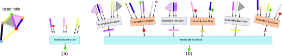
Figure 1: Two layers cell complex neural network (CXN) Hajij et al. (2020a) illustrated on a simplicial complex. The computations are illustrated with respect to the green target vertex.

3.2 Co-adjacency Message Passing Scheme (CMPS)

Co-adjacency message passing scheme is very similar to the AMPS we mentioned in Section 3. The only difference is that it utilizes the co-adjacency relations of a given face instead of the adjacency matrix. Specifically, let $H^{(0)}_{m}\in\mathbb{R}^{|X^{m}|\times d_{0}}$ be the initial cell feature vector on every $m$-cell in $X$. Let $L>0$ be the desired depth of the CXN one wants to define on a complex $X$, the Coadjacency Message Passing Scheme (CMPS) on $X$ consists of $L\times n$ embeddings and it is defined as

$$H^{(k)}_{n-m}:=M\left(A_{co},\mathbf{\partial}^{T},H^{(k-1)}_{n-m},H^{(k-1)}_{n-m-1};\theta^{(k)}_{n-m}\right),$$ (2)

where $0\leq m\leq n-1$, $1\leq k\leq L$, $H^{(k)}_{n-m}\in\mathbb{R}^{|X^{n-m}|\times d_{k}}$ are the embeddings computed after $k$ steps of applying Equation equation 2, $\mathbf{\partial}^{T}$ are the coboundary operators needed for the computations, and $\theta^{(k)}_{n-m}$ is a trainable weight vector at the layer $k$, $M$ is the message propagation function that depends on the weights $\theta^{(k)}_{n-m}$, the cell embeddings $H^{(k)}_{n-m}$ and the adjacency matrix of $X$. Observe also that the matrix $A_{adj}$ can be replaced by a version of the k-Hodge Laplacian matrix as well Roddenberry et al. (2021). See Figure 2 for an illustration of such message passing scheme on a simplicial complex.

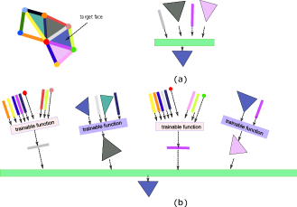
Figure 2: Coadjacency message passing scheme. The above illustrates the computation of a two layer cell complex network with respect the specified target face.

Note that with CMPS, the flow of information goes from higher cells to lower ones. This explains the strange index choice in Equation equation 2. Moreover, note that the feature vectors associated with the zero-cells are never updated.

3.3 Homology and Cohomology Message Passing Scheme (HCMPS)

Finally, the Homology and Cohomolgy Message Passing Scheme (HCMPS) is given by

$$H^{(k)}_{m}:=M\left(\partial,\mathbf{\partial}^{T},H^{(k-1)}_{m-1},H^{(k-1)}_{m+1};\theta^{(k)}_{m}\right),$$ (3)

where $0\leq m\leq n-1$, $1\leq k\leq L$, $H^{(k)}_{m}\in\mathbb{R}^{|X^{m}|\times d_{k}}$ are the embeddings computed after $k$ steps of applying Equation equation 3, $\partial,\mathbf{\partial}^{T}$ are the boundary and coboundary operators of the input complex. An example of applying the HCMPS is given in Figure 3.

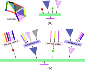
Figure 3: Homology and cohomology message passing scheme. The figure illustrates the computation of a two layers cell complex network with respect the specified edge.

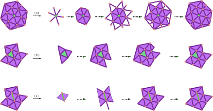
Figure 4: Illustration of the flow of information with various geometric message passing schemes (GMPS). (a) Flow of information with adjacency message passing schemes (AMPS). (b) Flow of information with co-adjacency message passing scheme (CMPS). (c) Flow of information with homology and cohomology message passing scheme (HCMPS). In all examples, the computations flow is given from the green simplex.

4 Entire Simplicial Complex Learning

Our proposed method for learning entire simplicial complex representation relies on collecting node-level simplicial representation and combining them together in order to obtain simplicial complex-level representation. In this section, we review the AMPS-simplicial autoencoder introduced in Hajij et al. (2020a). We then show how it can be utilized to obtain an entire-level simplicial representation by using metric learning.

4.1 Simplicial Complex AutoEncoders (SCAs)

Let $X$ be a simplicial complex of dimension $n$. A simplicial complex autoencoder (SCA) on $X$ consists of three components, namely of an encoder-decoder system, a user-defined similarity measure, and a user-defined loss function Hamilton et al. (2017b); Hajij et al. (2020a).

Firstly, the SCA encoder-decoder system is described. The encoder is a function of the form : $enc:X^{<n}\to\mathbb{R}^{d}$ and it associates to every $k-$ simplex $a^{k}$ in $X$ an embedding $\textbf{z}_{{a}^{k}}$ in $\mathbb{R}^{d}$. The decoder is a function of the form : $dec:\mathbb{R}^{d}\times\mathbb{R}^{d}\to\mathbb{R}^{+}$ and it associates to every pair of simplex embeddings $(\textbf{z}_{a^{k}},\textbf{z}_{c^{l}})$ a measure of similarity $dec(\textbf{z}_{a^{k}}\textbf{z}_{c^{l}})$ that quantifies some notion of relationship between $a^{k}$ and ${c^{l}}$. The functions $enc$ and $dec$ are trainable functions. In particular, the encoder can be chosen to be a cell complex network as illustrated in Section 3.

Secondly, a user-defined similarity measure is required by a SCA. We seek to train the encoder-decoder functions such that the trained similarity is as close as possible to the user-defined similarity: $dec(enc(a^{k}),enc(c^{l}))=dec(\textbf{z}_{a^{k}},\textbf{z}_{c^{l}})\approx sim_{X}(a^{k},c^{l}),$ where $sim_{X}:X^{<n}\times X^{<n}\to\mathbb{R}^{+}$ is a user-defined function such that $sim_{X}(a^{k},c^{l})$ reflects a user-defined similarity between the two simplicies $a^{k}$ and $c^{l}$ in $X^{<n}$. For instance, the similarity measure function on $X$ can be simply chosen the adjacency matrix $A_{adj}$ defined in Section 3.

Thirdly, a user-defined loss function is required by a SCA. Training the encoder-decoder system is done by specifying a loss function $l:\mathbb{R}\times\mathbb{R}\to\mathbb{R}$ and by defining

$$\mathcal{L}_{k}:=\sum_{\mathcal{CO}[a^{k},c^{k}]}l\left(dec(enc(\textbf{z}_{a^{k}}),enc(\textbf{z}_{c^{k}})),sim(a^{k},c^{k})\right)$$ (4)

and $\mathcal{L}:=\sum_{k=0}^{n-1}\mathcal{L}_{k}$. The sum in Equation equation 4 is taken over all possible $\mathcal{CO}[a^{k},c^{k}]\subset X^{k+1}$.

Table 1 shows several concert methods to define the autoencoders on simplicial complexes. Observe that any variant of the geometric message passing protocols can be used with any of the proposed simplicial complex autoencoders.

.

Table 1: Various definitions of simplicial somplex autoEncoders.

Method Decoder similarity Loss Laplacian eigenmaps Belkin & Niyogi (2001) $||\textbf{z}_{a}-\textbf{z}_{c}||_{2}^{2}$ general $dec(\textbf{z}_{a},\textbf{z}_{c}).sim(a,c)$ Inner product methods Ahmed et al. (2013) $\textbf{z}_{a}^{T}\textbf{z}_{c}$ $A_{adj}(a,c)$ $||dec(\textbf{z}_{a},\textbf{z}_{c})-sim(a,c)||_{2}^{2}$ Random walk methods Grover & Leskovec (2016); Perozzi et al. (2014) $\frac{e^{\textbf{z}_{a}^{T}\textbf{z}_{c}}}{\sum_{b\in X^{k}}e^{\textbf{z}_{a}^{T}\textbf{z}_{b}}}$ $p_{X}(a|c)$ $-log(dec(\textbf{z}_{a},\textbf{z}_{c}))$

4.2 Learning Entire Simplicial Complex Embedding

Let $enc:X^{<n}\to\mathbb{R}^{d}$ be a simplicial complex encoder. Denote by $\mathcal{U}_{X}\in\mathbb{R}^{\hat{N}\times d}$ to the simplices embeddings of $X^{<n}$ that are induced by the function $enc$. Our proposed method relies on learning a weighted sum of the simplex-level representations encoded in $\mathcal{U}_{X}$. Specifically, we seek to learn a simplicial complex-level embedding of the form

$$\mathbf{h}_{X}=\sum_{m=1}^{\hat{N}}w_{m}(\mathcal{U}_{X};W)\textbf{z}_{m},$$ (5)

where $w_{m}(\mathcal{U}_{X};W)\in\mathbb{R}$ is a weight of the simplex embedding $\textbf{z}_{m}$ that depends on $\mathcal{U}_{X}$ and parametrized by $W\in\mathbb{R}^{d\times d}$, a trainable weight matrix . The weight $w_{m}$ can be chosen in many different ways, here we simply follow Bai et al. (2019) and define the weight as

$$w_{m}(\mathcal{U}_{X};W)=\sigma\left((\textbf{z}_{m})^{T}\mathrm{RELU}\left(W\sum_{n=1}^{\hat{N}}\textbf{z}_{n}\right)\right),$$ (6)

where $\sigma(x)=\frac{1}{1+exp(-x)}$. Finally, the embedding $\mathbf{h}_{X}$ can be learned in multiple ways. For instance, given a collection of simplicial complex $\{X_{i}\}_{i=1}^{m}$ one may learn complex-to-complex proximity embeddings by minimizing the objective

$$\mathcal{L}=\sum_{i=1}^{m}\sum_{j=1}^{m}\left(||h_{X_{i}}-h_{X_{j}}||-d_{ij}\right)^{2},$$ (7)

where $D=[d_{ij}]$ is an appropriately chosen distance matrix on the simplicial complexes $\{X_{i}\}_{i=1}^{m}$. For example, the Haussdorf distance on simplicial complexes Marin (2020) can be employed to compute the distance matrix $D$. Alternatively, in special case when the simplicial complex is a triangulated mesh, more efficient methods to compute the metrics can be utilized such as persistence homology-based metrics Hajij et al. (2020b); Zhang et al. (2019) or Laplacian-based methods Crane et al. (2013).

5 Experiments

To test our proposed method, we train an AMPS-SCA on a publicly available datset. Initially, we experiment on a mesh dataset to help making a visual inspection of the SCA performance. This dataset, which is described in details in Sumner & Popović (2004), consists of 60 meshes that belong to 6 categories: cat, elephant, face, head, horse, and lion. Each category contains ten triangulated meshes. We train the model on the faces, heads, horses (total of thirty meshes); the rest of the dataset (i.e., elephants, horses and cats) were used to for testing. The model was trained using our PyTorch-based implementation. The final model consist of an AMPS single layer model that we described in Equation equation 1 with one additional dense layer at the end that operates on the vector $\mathbf{h}_{X}$. The model was trained using SGD techniques for $100$ epochs with a batch size of $1$; roughly, the model sees each model in the training dataset around three times. The final embedding dimension of the input mesh was chosen to be $2$ for visualization purposes. The results are shown in Figure 5. From the figure, we can observe that the model successfully clusters meshes with the same category close to each other. Moreover, meshes with related structure, quadruple animals, are also embedded in a spatially close neighborhood.

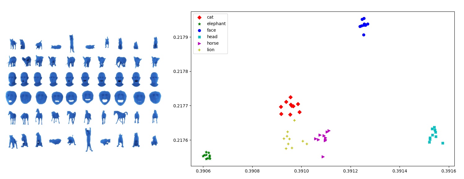
Figure 5: Initial results using our proposed simplicial complex autoencoder. The figure shows the entire simplicial complex embeddings of the whole dataset. The final embedding was chosen to be in $\mathbb{R}^{2}$. The model was trained on faces, heads, and horses. The inference indicated in the figure shows the entire embeddings for the 60 meshes. Note that while the model was never trained on the cat, camel and elephant meshes, it succeeded in clustering these meshes. Moreover, all animals with similar shapes are clustered together.

6 Discussion

In Section 4.2, we describe one way to learn the embeddings $\mathbf{h}_{X}$ in an unsupervised fashion. The method learns the proximity between simplical complexes that is encoded in a pre-computed matrix $D$ on a dataset of simplicial complexes. The problem with this method is that it requires the computation of the entire distance matrix which might be computationally inefficient. There are many other potentially good methods to learn such embeddings in an end-to-end fashion. For instance, a potential method to learn the metric of simplicial complex embeddings can be done by utilizing triplet loss method as proposed in Hoffer & Ailon (2015). Metric learning with the triplet loss method construct a triplet net which consists of three shared parameter feedforward networks. The network is fed three embeddings $\mathbf{h}_{X}$, $\mathbf{h}_{X^{+}}$ and $\mathbf{h}_{X^{-}}$ where $\mathbf{h}_{X}$ and $\mathbf{h}_{X^{+}}$ are of the same class, and $\mathbf{h}_{X}$ and $\mathbf{h}_{X^{-}}$ are of different class. We stress here the fact that while a binary label is utilized when choosing the triplet $(X,X^{+},X^{-})$, triplet network can effectively learn a metric and determine which simplicial complexes are closer to a given complex $X$. In other words, the interpretation of sharing the same class is correlated with embedding closeness in the embedding space Hoffer & Ailon (2015). The advantages of the triplet loss method is that we do not need to pre-compute a distance matrix on the simplicial complexes training set. However, the triplet loss method requires a labeled training dataset which might not be always available.

References

- Ahmed et al. (2013) Amr Ahmed, Nino Shervashidze, Shravan Narayanamurthy, Vanja Josifovski, and Alexander J Smola. Distributed large-scale natural graph factorization. In Proceedings of the 22nd international conference on World Wide Web, pp. 37–48, 2013.
- Angles & Gutierrez (2008) Renzo Angles and Claudio Gutierrez. Survey of graph database models. ACM Computing Surveys (CSUR), 40(1):1–39, 2008.
- Bai et al. (2019) Yunsheng Bai, Hao Ding, Yang Qiao, Agustin Marinovic, Ken Gu, Ting Chen, Yizhou Sun, and Wei Wang. Unsupervised inductive graph-level representation learning via graph-graph proximity. In IJCAI’19, pp. 1988–1994. AAAI Press, 2019.
- Belkin & Niyogi (2001) Mikhail Belkin and Partha Niyogi. Laplacian eigenmaps and spectral techniques for embedding and clustering. Advances in neural information processing systems, 14:585–591, 2001.
- Billings et al. (2019) Jacob Charles Wright Billings, Mirko Hu, Giulia Lerda, Alexey N Medvedev, Francesco Mottes, Adrian Onicas, Andrea Santoro, and Giovanni Petri. Simplex2vec embeddings for community detection in simplicial complexes. arXiv preprint arXiv:1906.09068, 2019.
- Chen & Koga (2019) Hong Chen and Hisashi Koga. Gl2vec: Graph embedding enriched by line graphs with edge features. In International Conference on Neural Information Processing, pp. 3–14. Springer, 2019.
- Crane et al. (2013) Keenan Crane, Clarisse Weischedel, and Max Wardetzky. Geodesics in heat: A new approach to computing distance based on heat flow. ACM Transactions on Graphics (TOG), 32(5):1–11, 2013.
- Cui et al. (2018) Peng Cui, Xiao Wang, Jian Pei, and Wenwu Zhu. A survey on network embedding. IEEE Transactions on Knowledge and Data Engineering, 31(5):833–852, 2018.
- de Lara & Pineau (2018) Nathan de Lara and Edouard Pineau. A simple baseline algorithm for graph classification. arXiv preprint arXiv:1810.09155, 2018.
- Ebli et al. (2020) Stefania Ebli, Michaël Defferrard, and Gard Spreemann. Simplicial neural networks. NeurIPS 2020 Workshop TDA and Beyond, 2020.
- Fey & Lenssen (2019) Matthias Fey and Jan Eric Lenssen. Fast graph representation learning with pytorch geometric. arXiv preprint arXiv:1903.02428, 2019.
- Glaze et al. (2021) Nicholas Glaze, T Mitchell Roddenberry, and Santiago Segarra. Principled simplicial neural networks for trajectory prediction. arXiv preprint arXiv:2102.10058, 2021.
- Grover & Leskovec (2016) Aditya Grover and Jure Leskovec. node2vec: Scalable feature learning for networks. In Proceedings of the 22nd ACM SIGKDD international conference on Knowledge discovery and data mining, pp. 855–864, 2016.
- Hacker (2020) Celia Hacker. k-simplex2vec: a simplicial extension of node2vec. NeurIPS workshop on Topological Data Analysis and Beyond, 2020.
- Hajij et al. (2018) Mustafa Hajij, Bei Wang, Carlos Scheidegger, and Paul Rosen. Visual detection of structural changes in time-varying graphs using persistent homology. In 2018 IEEE Pacific Visualization Symposium (PacificVis), pp. 125–134. IEEE, 2018.
- Hajij et al. (2020a) Mustafa Hajij, Kyle Istvan, and Ghada Zamzmi. Cell complex neural networks. NeurIPS 2020 Workshop TDA and Beyond, 2020a.
- Hajij et al. (2020b) Mustafa Hajij, Elizabeth Munch, and Paul Rosen. Fast and scalable complex network descriptor using pagerank and persistent homology. In 2020 International Conference on Intelligent Data Science Technologies and Applications (IDSTA), pp. 110–114. IEEE, 2020b.
- Hamilton et al. (2017a) William L Hamilton, Rex Ying, and Jure Leskovec. Inductive representation learning on large graphs. arXiv preprint arXiv:1706.02216, 2017a.
- Hamilton et al. (2017b) William L Hamilton, Rex Ying, and Jure Leskovec. Representation learning on graphs: Methods and applications. arXiv preprint arXiv:1709.05584, 2017b.
- Hatcher (2005) Allen Hatcher. Algebraic topology. Cambridge University Press, 2005.
- Heimann et al. (2018) Mark Heimann, Haoming Shen, Tara Safavi, and Danai Koutra. Regal: Representation learning-based graph alignment. In Proceedings of the 27th ACM international conference on information and knowledge management, pp. 117–126, 2018.
- Hoffer & Ailon (2015) Elad Hoffer and Nir Ailon. Deep metric learning using triplet network. In International workshop on similarity-based pattern recognition, pp. 84–92. Springer, 2015.
- Kipf & Welling (2016) Thomas N Kipf and Max Welling. Semi-supervised classification with graph convolutional networks. arXiv preprint arXiv:1609.02907, 2016.
- Love et al. (2021) E R Love, B Filippenko, V Maroulas, and G Carlsson. Toplogical deep learning. arXiv:2101.05778, 2021.
- Marin (2020) Ivan Marin. Hausdorff metric between simplicial complexes. arXiv preprint arXiv:2001.11707, 2020.
- Maroulas et al. (2019) Vasileios Maroulas, Joshua Mike, and Christopher Oballe. Nonparametric estimation of probability density functions of random persistence diagrams. Journal of Machine Learning Research, 20(151):1–49, 2019.
- Maroulas et al. (2021) Vasileios Maroulas, Cassie Putman Micucci, and Farzana Nasrin. Bayesian Topological Learning for Classifying the Structure of Biological Networks. Bayesian Analysis, pp. 1 – 26, 2021. doi: 10.1214/21-BA1270.
- Mikolov et al. (2013) Tomas Mikolov, Kai Chen, Greg Corrado, and Jeffrey Dean. Efficient estimation of word representations in vector space. arXiv preprint arXiv:1301.3781, 2013.
- Narayanan et al. (2017) Annamalai Narayanan, Mahinthan Chandramohan, Rajasekar Venkatesan, Lihui Chen, Yang Liu, and Shantanu Jaiswal. graph2vec: Learning distributed representations of graphs. arXiv preprint arXiv:1707.05005, 2017.
- Nasrin et al. (2019) Farzana Nasrin, Christopher Oballe, David Boothe, and Vasileios Maroulas. Bayesian topological learning for brain state classification. In 2019 18th IEEE International Conference On Machine Learning And Applications (ICMLA), pp. 1247–1252, 2019.
- Oballe et al. (2021) Christopher Oballe, David Boothe, Piotr J. Franaszczuk, and Vasileios Maroulas. Tofu: Topology functional units for deep learning. Foundations of Data Science, 2021. doi: 10.3934/fods.2021021.
- Perozzi et al. (2014) Bryan Perozzi, Rami Al-Rfou, and Steven Skiena. Deepwalk: Online learning of social representations. In Proceedings of the 20th ACM SIGKDD international conference on Knowledge discovery and data mining, pp. 701–710, 2014.
- Roddenberry et al. (2021) T Mitchell Roddenberry, Michael T Schaub, and Mustafa Hajij. Signal processing on cell complexes. arXiv preprint arXiv:2110.05614, 2021.
- Schaub et al. (2020) Michael T Schaub, Austin R Benson, Paul Horn, Gabor Lippner, and Ali Jadbabaie. Random walks on simplicial complexes and the normalized hodge 1-laplacian. SIAM Review, 62(2):353–391, 2020.
- Sumner & Popović (2004) Robert W Sumner and Jovan Popović. Deformation transfer for triangle meshes. ACM Transactions on graphics (TOG), 23(3):399–405, 2004.
- Tang et al. (2019) E. Tang, M.G. Mattar, C. Giusti, and et al. Effective learning is accompanied by high-dimensional and efficient representations of neural activity. Nat Neurosci, 22:1000–1009, 2019.
- Tsitsulin et al. (2018) Anton Tsitsulin, Davide Mottin, Panagiotis Karras, Alexander Bronstein, and Emmanuel Müller. Netlsd: hearing the shape of a graph. In Proceedings of the 24th ACM SIGKDD International Conference on Knowledge Discovery & Data Mining, pp. 2347–2356, 2018.
- Ying et al. (2018) Rex Ying, Jiaxuan You, Christopher Morris, Xiang Ren, William L Hamilton, and Jure Leskovec. Hierarchical graph representation learning with differentiable pooling. arXiv preprint arXiv:1806.08804, 2018.
- Zhang et al. (2019) Yunhao Zhang, Haowen Liu, Paul Rosen, and Mustafa Hajij. Mesh learning using persistent homology on the laplacian eigenfunctions. arXiv preprint arXiv:1904.09639, 2019.