Controlling Thermal Convection with Side Heating

Abstract

In Rayleigh-Bénard convection, a fluid volume is heated from below and cooled at the top. Due to buoyancy forces, hot fluid rises and cold fluid sinks, leading to an overall upward heat flux that has a power-law dependence on the imposed temperature difference. Our experiment shows that, adding sidewall heating modifies this power-law relation, thus brings control to this classical fluidic system. Through careful flow, temperature, and heat flux measurements, we investigate the effects of such side-heating to Rayleigh-Bénard convection and rationalize our observations with simple relations that describe how side-heating controls the overall heat transfer. Such control-response mechanism is conceptually analogous to that of electrical transistors, and our “thermal transistor" may serve as a potential building block for more complex thermal-fluidic circuits.

As a model system, Rayleigh-Bénard convection (RBC) has been extensively studied [1, 2, 3, 4, 5, 6], for its vastly broad applications in geophysics [7, 8, 9], solar physics [10, 11], atmospheric science [12, 13], ocean dynamics [12, 14], and many industrial processes [15]. In RBC, a domain of fluid is heated from below and cooled at the top, which causes hot fluid to ascend and cold fluid to descend. As the the warm and cold fluids move between the top and bottom plates, they effectively create an upward heat flux passing through the domain. At a fixed bottom-to-top temperature difference, this convective heat transfer rate $Q_{conv}$ is much greater than that would pass through a quiescent fluid body, $Q_{cond}$, the so-called conductive heat transfer rate. Defined as the ratio between the convective and conductive heat transfer rates, the Nusselt number $\mbox{Nu}=Q_{conv}/Q_{cond}$ measures the heat-passing capability in RBC, which depends on imposed control parameters such as the Rayleigh number, $\mbox{Ra}=\alpha gL^{3}\Delta T/\kappa\nu$, and the Prandtl number, $\mbox{Pr}=\nu/\kappa$. Here, $\Delta T$ is the imposed top-bottom temperature difference, and constants $g,L,\alpha,\kappa,\nu$ are the acceleration due to gravity, fluid depth, thermal expansion coefficient, thermal diffusivity and kinematic viscosity, respectively.

Once a fluid and its containing geometry are given, the heat flux is uniquely determined by the imposed temperature difference $\Delta T$. In particular, the famous scaling relationship $\mbox{Nu}\propto\mbox{Ra}^{\beta}$ with an exponent $\beta\approx 1/3$ has been observed in the range from $\mbox{Ra}=10^{6}$ to $\mbox{Ra}=10^{14}$ [3, 4], despite local deviations. Grossmann and Lohse [16, 5, 17] developed a theory – the GL theory – that incorporates the heat transfer contributed by the thermal boundary layers and the bulk, reveals the Nu-Ra relationship, and has been found to be consistent with many experiments [18, 5].

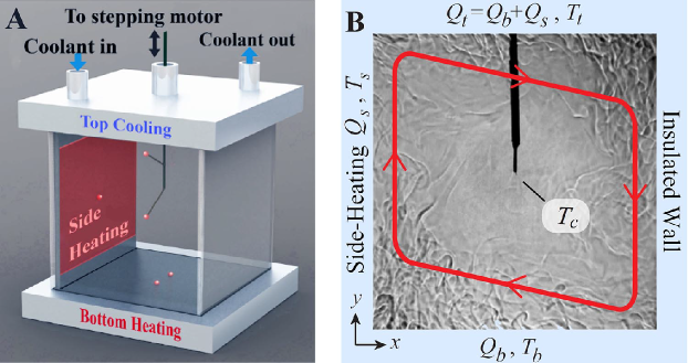
Figure 1: Cubical thermal convection cell with sidewall heating is filled with water as the working fluid. (A) Schematic showing the convection cell, side heater and thermistors (red dots) distributed to measure local temperature at various locations. (B) Shadowgraph visualizing the density differences and thus the flow structures, with bottom heating power $Q_{b}=100$ W and side-heating power $Q_{s}=40$ W. Heat injected from the bottom and the side exits the fluid through the top cooling plate, while the clockwise large-scale circulation is enhanced and dictated by the side-heating.

The monotonic dependency of Nu on Ra, or more directly of $Q_{conv}$ on $\Delta T$, is analogous to the dependency an electrical current has on an imposed voltage over a resistive element. Indeed, the Nu-Ra dependency is not linear, unlike any Ohmic material in electronics. At an imposed Rayleigh number, a controllable Nu or heat flux is often desired; anomalies that deviate from the usual scaling laws found in nature also demand explanations [19]. In the past, there have been attempts to modify the Nu-Ra dependency. For example, surface roughness was added to the heating/cooling plate that changes the boundary layer structure [20, 21], which enhances the Nusselt number. Adding rotation to the entire fluid changes the bulk flow structure [22, 23, 24] and increases the Nusselt number at moderate rotation rate. Stronger confinement on the convective fluid increases the flow structure coherence [25, 26, 27], and leads to higher Nusselt number. Horizontal vibration is also observed to disrupt the boundary layer structure and increase the Nusselt number significantly [28]. Bao et al. reported a strong Nu enhancement when vertical partition walls are inserted in the bulk fluid [29]. There, convective fluid self-organizes and circulates around these partitions, intruding the thermal boundary layers and leading to greatly increased heat flux.

Inspired by the fact that a horizontal temperature gradient induces enhanced bulk circulation in RBC [30], we aim to control the vertical heat flux by adding a sidewall heating. In this study, a classical RBC system in a cubical domain is perturbed by a heat flux injected from one of its four vertical sides, see Fig. 1. During each experiment, the top cooling temperature $T_{t}$ is fixed, and Ra and Nu numbers are measured as functions of the side and bottom heating powers $Q_{s}$ and $Q_{b}$. To the best of our knowledge, this unconventional configuration, which resembles an oversized electronic transistor (in that one flux controls another flux), has not been studied in the past. Indeed, many experiments have explored configurations such as sidewall heating-cooling without bottom heating [30], horizontal convection [31, 32, 33], and different sidewall boundary conditions [34]. Our goal is to find a simple means to control the vertical heat transfer rate $Q_{b}$ under perturbation $Q_{s}$.

As shown in Fig. 1A, our experiments are carried out in a cubical cell that has dimension $L=20$ cm on each side. The top and bottom plates are made of anodized aluminum that ensures high thermal conductivity and uniform temperature distribution within each plate. In the top plate, coolant water is circulated at a constant temperature $40^{\circ}$C that is regulated by a water circulator. An electrical film heater is embedded in the bottom plate of RBC, providing bottom heating to the fluid. Another film heater covered by an aluminum sheet, 2 mm in thickness, is attached to one side of the vertical walls. The use of the aluminum sheet is intended to improve temperature uniformity on this wall, and its top and bottom edges are cut away by 5 mm in order to prevent a “short circuit” of heat flowing from/to the bottom/top boundary layers. All other vertical walls are transparent to allow flow visualization. During all experiments excluding flow visualization, insulating materials cover the RBC cell to minimize heat leak. Local temperatures are measured with thermistors distributed in the convection cell. As shown in Fig. 1A, two thermistors, measuring the bottom temperature (labeled as red dots), are embedded 0.5 mm below the bottom surface. One thermistor is located at the center of the side heater to monitor the side temperature, and two thermistors are mounted on a support that can traverse vertically to measure vertical temperature profiles.

We perform all temperature and flow speed measurements at each $(Q_{b},Q_{s})$, while varying them independently in the range of 0 to 120 W. Whenever a control parameter (e.g., the side-heating power) is changed, the system runs for 4 hours to reach dynamic equilibrium, and each measurement takes another 4 hours to collect data. With degassed water as the working fluid, the system works at Rayleigh number in the range of $3\times 10^{8}$ to $5\times 10^{9}$ and Prandtl number in the range of $3.4$ to $4.1$, a turbulent regime that is often accompanied with a large-scale circulation (LSC).

A shadowgraph of the convection cell reveals local density differences of the fluid and thus allows visualization of the convective flows. A convex lens with focal length 20 cm converts light from a point source to near-parallel light, which passes through the convection cell and casts a shadow on a translucent screen. A typical shadowgraph image is shown in Fig. 1B. Bulk flow speed $U$ can be inferred from tracing thermal plumes at a given region of the recorded video. Typically, trajectories of 40 plumes are timed and metered during each experiment, flow speeds and error bar are then recorded.

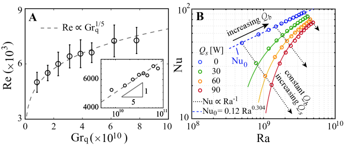
Figure 2: Flow speed and heat transfer measured by Reynolds and Nusselt numbers. (A) Plume speed and that of LSC increase with side-heating power. With bottom heating fixed at 100 W, Reynolds number $\mbox{Re}=UL/\nu$ measured close to the sidewall shows a monotonic dependence on the power Grashof number Gr_q, consistent with the power-law $\mbox{Re}\propto\mbox{Gr}_{q}^{1/5}$ from the boundary layer theory [35]. Inset: Logarithmic-scale plot of Reynolds number and power Grashof number. (B) Nusselt number Nu measured at various Rayleigh number Ra and side-heating power $Q_{s}$. The bottom heating power is $Q_{b}=10,20,\dots 120$ W. Without side-heating, Nu shows a classical power-law dependence on Ra. Fixing the bottom power, Nu is observed to decrease with increasing side power, while Nu $\propto$ Ra^-1. Colored solid curves are the Nu-Ra curve at each $Q_{s}$ predicted by a theory introduced later.

We expect that side-heating enhances the LSC, and perhaps also increases the vertical heat transfer rate. Indeed, the heated fluid is lighter around the side heater and forms an upwelling jet, which dictates the LSC as indicated in Fig. 1B. Here, the thermal energy is partially converted into the fluid kinetic energy of the LSC and partially stored in the bulk.

With a constant bottom heating power $Q_{b}=100$ W and side-heating power in the range of $Q_{s}=10-100$ W, the flow speed can be nondimensionalized as the Reynolds number $\mbox{Re}=UL/\nu$ in the bulk. The sidewall power can be represented by the power Grashof number $\mbox{Gr}_{q}=\alpha gL^{2}Q_{s}/\lambda\nu^{2}$, which is a measure of relative strength between the buoyancy force due to heating and that of viscosity [35]. Here, $\lambda$ is the thermal conductivity of the fluid. In comparison with the Grashof number $\mbox{Gr}=\alpha gL^{3}(T_{s}-T_{\infty})/\nu^{2}$, the power Grashof number is defined directly through the input heating power $Q_{s}$ instead of the heating-power-induced temperature difference $T_{s}-T_{\infty}$. The far field temperature $T_{\infty}$ in our case can be regarded as the bulk temperature, $T_{\infty}=T_{c}$.

The dependence of Re on the side-heating strength is shown in Fig. 2A. The monotonic increase of Re with Gr_q shows that the bulk flow speed is indeed accelerated by the side-heating power. From the boundary layer theory [35], the buoyancy-driven flow speed near a vertical wall scales with the Grashof number Gr as $U\propto\mbox{Gr}^{1/4}$. Using the relationship between the two Grashof numbers [35], namely $\mbox{Gr}\propto\mbox{Gr}_{q}^{4/5}$, we have the scaling law $\mbox{Re}(U)\propto\mbox{Gr}^{1/4}\propto\mbox{Gr}_{q}^{1/5}$. This is found to be consistent with our experimental data, as shown in Fig. 2A. As $Q_{s}$ reduces to 0, flow velocity drops to the conventional LSC value, which corresponds to Re $\sim 1000$ in our range of Ra [5], and the direction of LSC becomes arbitrary but along the diagonal planes of the convection cell.

The Nusselt number in the classical cubical RBC is Nu $=Q_{b}/\lambda\Delta TL$, which measures the vertical heat-passing capability. Figure 2B shows the Nusselt number measured at various $Q_{s}$ and $Q_{b}$. With sidewall heating added, the bulk circulation is enhanced as expected, but the bottom temperature $T_{b}$ and thus $\Delta T=T_{b}-T_{t}$ are found to increase. By definition Ra $\propto\Delta T$ and Nu $\propto 1/\Delta T$, so an increased $\Delta T$ due to side-heating causes Ra to increase and Nu to decrease. Moreover, with $Q_{b}$ fixed at a constant, the product Nu$\cdot$Ra is a constant that contains only fluid properties and fluid depth. Thus, the dotted lines in Fig. 2B have a common slope -1 in the log-log scale.

As a reference, the Nu-Ra measurement (Fig. 2B) with no sidewall heating Nu$|_{Q_{s}=0}=\mbox{Nu}_{0}$ shows good agreement with that from previous experiments [4, 5]. This is evident by plotting our data together with the power-law $\mbox{Nu}=0.12\mbox{Ra}^{0.304}$, which is a scaling relationship suggested by the GL theory in our range of Ra. When $Q_{s}\neq 0$, the observed data deviate from the power-law relation – a simple scaling relationship is absent, particularly at large $Q_{s}$. Such trend can also be seen in the numerical simulations for a wide range of Ra (Supplemental Information).

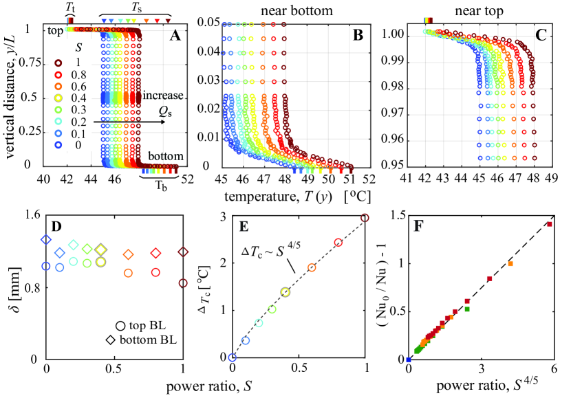
Figure 3: Vertical temperature profiles measured at $Q_{b}=100$ W and various $Q_{s}$. Measurements are taken along the center vertical line as shown in Fig. 1A. (A) Temperature measured throughout the cell. The bulk and bottom temperatures are found to rise with the heating power ratio $S=Q_{s}/Q_{b}$. Top, bottom and side temperatures ($T_{t},T_{b}$ and $T_{s}$) are marked with ticks and triangles. (B) Zoom-in profiles of the bottom boundary layer. $T_{b}$ increases with the bulk temperature, while the temperature gradient at bottom stays nearly constant. (C) Zoom-in profiles of the top boundary layer. With top temperature fixed, increased bulk temperature leads to a higher temperature gradient within the boundary layer. (D) Thermal boundary layer thicknesses $\delta$ of the top and bottom boundary layers. (E) With $Q_{b}$ fixed, the increase of bulk temperature $\Delta T_{c}=T_{c}|_{S}-T_{c}|_{S=0}$ has a $4/5$ power-law scaling relationship to the side-heating power $Q_{s}$. (F) Nusselt number as a function of power ratio $S$, $\mbox{Nu}_{0}/\mbox{Nu}=1+\frac{1}{4}S^{4/5}$. [(A)-(E) share the same color scheme; (F) has the same color scheme and definition of Nu and Nu₀ as in Fig. 2B]

To rationalize the changed Nu-Ra relationship due to sidewall heating, the vertical temperature profiles are carefully examined. Fig. 3A shows several profiles that have the same bottom power $Q_{b}=100$ W but different side power $Q_{s}$. The heating power ratio is defined as $S=Q_{s}/Q_{b}$. Among all these curves, temperature changes linearly within thermal boundary layers next to the top and bottom plates, through which heat transfers by diffusion. In the bulk, the time-averaged temperature remains nearly uniform at $T_{c}$, which, together with the bottom temperature $T_{b}$, rises with increasing $Q_{s}$.

Zooming in near the bottom, Fig. 3B shows that the bottom temperature $T_{b}$ increases with $Q_{s}$ while the temperature gradient $\partial T/\partial y$ stays roughly constant within the boundary layer. This is due to the fact that $\partial T/\partial y=-Q_{b}/\lambda L^{2}$ and the bottom power $Q_{b}$ is fixed at a constant. The bottom boundary layer thickness $\delta_{b}=1.4\pm 0.1$ mm or $\delta_{b}/L=(0.70\pm 0.05)\%$ is roughly constant for various $S$ as shown in Fig. 3D. Since $\partial T/\partial y\sim\Delta T_{b}/\delta_{b}$, the temperature difference between the bottom and the center (bulk) $\Delta T_{b}=T_{b}-T_{c}$ is not changing with $S$ either, as shown in Fig. 3B. Figure 3C shows the zoom-in temperature profiles near the top plate. The addition of the side-heating $Q_{s}$, which has to leave the system through the top plate, leads to a higher temperature gradient $\partial T/\partial y=-(Q_{b}+Q_{s})/\lambda L^{2}$ at the top. In our experiment, the top boundary layer thickness $\delta_{t}=1.1\pm 0.1$ mm or $\delta_{t}/L=(0.55\pm 0.05)\%$ decreases slightly when $S$ increases, as shown in Fig. 3D. In the bulk, the temperature is nearly uniform because of strong mixing [2]. The value of this temperature increases with $S$ as shown in Fig. 3A and Fig. 3E.

As one focuses on $Q_{conv}$ and $Q_{cond}$ in the vertical direction, the only variable in Nu $=Q_{b}/\lambda\Delta TL$ is $\Delta T$ when holding $Q_{b}$ constant. From the observations shown in Fig. 3B, the bottom to bulk temperature difference stays unchanged while the bulk temperature increases with $S$. Therefore, the increase of bulk temperature $\Delta T_{c}(S)=T_{c}|_{S}-T_{c}|_{S=0}$ directly leads to an increased bottom-top temperature difference $\Delta T|_{S}=\Delta T|_{S=0}+\Delta T_{c}(S)$. The quantity $\Delta T_{c}(S)$ can be estimated by applying the sidewall boundary layer scaling $T_{s}-T_{c}\propto S^{4/5}$ ($\mbox{Gr}\propto\mbox{Gr}_{q}^{4/5}$), which gives $\Delta T_{s}-\Delta T_{c}\propto S^{4/5}$ since $T_{s}|_{S=0}=T_{c}|_{S=0}$. It is reasonable to assume that $\Delta T_{c}\propto\Delta T_{s}$, and consequently $\Delta T_{c}\propto S^{4/5}$. This relationship is indeed observed in Fig. 3E.

The bottom-top temperature difference now becomes $\Delta T=(1+\gamma S^{4/5})\Delta T|_{S=0}$, where $\gamma$ is a positive constant. Substituting this into the Nusselt number, we have $\mbox{Nu}_{0}/\mbox{Nu}(S)=\Delta T/\Delta T|_{S=0}=1+\gamma S^{4/5}$. Plotting $\mbox{Nu}_{0}/\mbox{Nu}-1$ against $S^{4/5}$, all the data points in Fig. 2B land on a straight line as shown in Fig. 3F, whose slope (a fitting parameter, see Supplemental Information) is $\gamma=1/4$. We can also apply this relation to $S=Q_{s}/Q_{b}$ with fixed $Q_{s}$ and varying $Q_{b}$, shown as the Ra-Nu curve for each $Q_{s}$ in Fig. 2B, agreeing well with the experimental data.

The above analysis provides a rationale relationship between the changed Nu and side-heating $S$, so the latter can be seen as a control to the vertical heat-passing capability. Adding side-heating apparently decreases Nu, when it is defined classically as one only focuses on the vertical heat transfer $Q_{b}$. This result seems to contradict the fact that side-heating enhances LSC and promotes overall mixing – effects known to increase heat exchange and heat transfer.

Below, we consider all heat inputs to the RBC system as the overall convective heat $Q^{*}_{conv}$, and compare it with the overall conductive heat $Q^{*}_{cond}$ that incorporates changed temperature fields when side-heating is present. The resulting analysis will show that the newly defined Nusselt number Nu${}^{*}=Q^{*}_{conv}/Q^{*}_{cond}$, is in fact increasing with $S$.

Indeed, the sum of the side and bottom heat has to flow out through the top plate. In terms of power, the total convective power through the cell is $Q^{*}_{conv}=Q_{t}=Q_{b}+Q_{s}$, here $Q_{t},\ Q_{b}$ and $Q_{s}$ represent the magnitude of power passing through the top, bottom and side, respectively. The side-heating also leads to a side temperature $T_{s}>T_{c}>T_{t}$ and it contributes to the total conductive heat flow through the top plate. Hence $Q_{cond}^{*}$ has to be redetermined by solving a steady state heat equation with $T_{b},\ T_{t}$ and $T_{s}$ satisfying Dirichlet boundary conditions for the bottom, top and one sidewall, and $\partial_{n}T=0$ satisfying the adiabatic condition on other 3 sidewalls. To prevent short-circuiting, the heating sidewall is separated into three regions, one central region with constant temperature $T_{s}$ and two stripes on its top and bottom with adiabatic boundary conditions, with the size matching the experimental configuration of $5:190:5\mbox{ mm}$. The steady-state heat equation $\partial_{x}^{2}T+\partial_{y}^{2}T=0$, satisfying these mixed boundary conditions, can be solved with numerical methods, e.g., finite differences and finite elements. Here we use a finite elements package COMSOL Multiphysics with MATLAB Livelink and compute the conductive heat in 2D, as we assume no significant structural changes in the third direction. The overall conductive heat transfer rate is thus determined as $Q^{*}_{cond}=-\lambda L\int_{0}^{L}\frac{\partial T}{\partial y}(x,L)dx$.

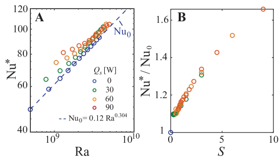
Figure 4: Redefined Nusselt number Nu^∗ (see text) as the ratio of total convective heat to total conductive heat. (A) With redefinition, data shown on Fig. 2B are now above the Ra-Nu₀ curve when $Q_{s}>0$, showing an enhancement of heat transfer. (B) The ratio Nu${}^{*}/$Nu₀ increases monotonically with the heating power ratio $S=Q_{s}/Q_{b}$, reaching the highest enhancement of $66\%$ at $S=9$ in the experiment. [(A)-(B) share the same color scheme as in Fig. 2B]

As shown in Fig. 4A, the redefined Nu${}^{*}=Q^{*}_{conv}/Q^{*}_{cond}$ for each Ra and $S$ lies above the unperturbed Ra-Nu₀ curve (dashed line in Fig. 4A), showing that side-heating and enhanced LSC indeed result in a higher heat transfer rate. This enhancement of Nu^∗ is also seen in numerical simulations (Supplemental Information). At large Ra (small $S$), contribution from the bottom heating $Q_{b}$ dominates the overall heat transfer, so the classical Nu₀-Ra relationship becomes the asymptotic limit. At small Ra (large $S$), however, the redefined Nu^∗ deviates from the power-law scaling when the side-heating presents. The degree of this enhancement, measured as Nu${}^{*}/$Nu₀, is plotted in Fig. 4B, where it increases monotonically with $S$ and reaches the highest enhancement of $66\%$ at $S=9$ in our experiments. We attribute this Nu^∗ boost to the strengthening of the large-scale circulation due to side-heating, which mixes temperature in the bulk more efficiently and perhaps thins the boundary layers (Fig. 3D). As an extreme example, the enhancement of Nu^∗ is most obvious when the system is around the critical Rayleigh number (Supplemental Information), as the side-heating initiates fluid motions in an otherwise non-convective, pure conductive system.

In electronics, NPN transistor is an element that has three leads termed emitter, base and collector. When a current $I_{B}$ flows into the base, the current flowing between collector and emitter $I_{E}$ increases (Supplemental Information). This forms the control-response mechanism of using NPN transistor in logic circuits. If we regard the Nusselt number Nu^∗ as $I_{E}$ and the side heating $S$ as $I_{B}$, the RBC system behaves exactly like a NPN electronic transistor with sidewall as the base, bottom wall as the collector and top wall as the emitter. In our thermal transistor, Nu^∗ increases when heat is added to the sidewall (higher $S$).

Like many other analogies between fluid and electronic systems, our thermal transistor functions like an electrical transistor as it controls a heat flux by introducing an additional heat input. Many questions regarding the feasibility of heat-flux control in other regimes of thermal convection and with complex geometries remain to be explored. Currently we are exploring the effect of a horizontal heat flux added to Rayleigh-Bénard convection – in addition to the side-heating, the same amount of heat is taken away from the opposite wall. Just like the way our current study introduces a thermal transistor, we aim to discover more elements for the thermal-fluidic circuits in the future.

References

- [1] Tilgner, A., Belmonte, A. & Libchaber, A. Temperature and velocity profiles of turbulent convection in water. \JournalTitlePhys. Rev. E 47, R2253 (1993).
- [2] Belmonte, A., Tilgner, A. & Libchaber, A. Temperature and velocity boundary layers in turbulent convection. \JournalTitlePhys. Rev. E 50, 269 (1994).
- [3] Niemela, J., Skrbek, L., Sreenivasan, K. & Donnelly, R. Turbulent convection at very high Rayleigh numbers. \JournalTitleNature 404, 837–840 (2000).
- [4] Funfschilling, D., Brown, E., Nikolaenko, A. & Ahlers, G. Heat transport by turbulent Rayleigh–Bénard convection in cylindrical samples with aspect ratio one and larger. \JournalTitleJ. Fluid Mech. 536, 145–154 (2005).
- [5] Ahlers, G., Grossmann, S. & Lohse, D. Heat transfer and large scale dynamics in turbulent Rayleigh-Bénard convection. \JournalTitleRev. Mod. Phys. 81, 503 (2009).
- [6] Lohse, D. & Xia, K.-Q. Small-scale properties of turbulent Rayleigh-Bénard convection. \JournalTitleAnnu. Rev. Fluid Mech. 42, 335–364, 10.1146/annurev.fluid.010908.165152 (2010).
- [7] Zhong, J.-Q. & Zhang, J. Thermal convection with a freely moving top boundary. \JournalTitlePhys. Fluids 17, 115105 (2005).
- [8] Meakin, P. & Jamtveit, B. Geological pattern formation by growth and dissolution in aqueous systems. \JournalTitleP. Roy. Soc. A-Math. Phy. 466, 659–694 (2010).
- [9] Huang, J. M., Zhong, J.-Q., Zhang, J. & Mertz, L. Stochastic dynamics of fluid–structure interaction in turbulent thermal convection. \JournalTitleJ. Fluid Mech. 854, R5, 10.1017/jfm.2018.683 (2018).
- [10] Nordlund, Å. Solar convection. \JournalTitleSol. Phys. 100, 209–235 (1985).
- [11] Stein, R. & Nordlund, Å. Topology of convection beneath the solar surface. \JournalTitleAstrophys. J. 342, L95–L98 (1989).
- [12] Vallis, G. K. Atmospheric and oceanic fluid dynamics (Cambridge University Press, 2017).
- [13] Emanuel, K. A. et al. Atmospheric convection (Oxford University Press, 1994).
- [14] Jorgensen, D. P. & LeMone, M. A. Vertical velocity characteristics of oceanic convection. \JournalTitleJ. Atmos. Sci. 46, 621–640 (1989).
- [15] Incropera, F. P., Lavine, A. S., Bergman, T. L. & DeWitt, D. P. Fundamentals of heat and mass transfer (Wiley, 2007).
- [16] Grossmann, S. & Lohse, D. Scaling in thermal convection: a unifying theory. \JournalTitleJ. Fluid Mech. 407, 27–56 (2000).
- [17] Stevens, R. J. A. M., van der Poel, E. P., Grossmann, S. & Lohse, D. The unifying theory of scaling in thermal convection: the updated prefactors. \JournalTitleJ. Fluid Mech. 730, 295–308, 10.1017/jfm.2013.298 (2013).
- [18] Grossmann, S. & Lohse, D. Scaling in thermal convection: a unifying theory. \JournalTitleJ. Fluid Mech. 407, 27–56, 10.1017/S0022112099007545 (2000).
- [19] Barry, R. G. Mountain weather and climate (Psychology Press, 1992).
- [20] Du, Y.-B. & Tong, P. Enhanced heat transport in turbulent convection over a rough surface. \JournalTitlePhys. Rev. Lett. 81, 987–990, 10.1103/PhysRevLett.81.987 (1998).
- [21] Jiang, H. et al. Controlling heat transport and flow structures in thermal turbulence using ratchet surfaces. \JournalTitlePhys. Rev. Lett. 120, 044501, 10.1103/PhysRevLett.120.044501 (2018).
- [22] Zhong, J.-Q. et al. Prandtl-, Rayleigh-, and Rossby-Number dependence of heat transport in turbulent rotating Rayleigh-Bénard convection. \JournalTitlePhys. Rev. Lett. 102, 044502, 10.1103/PhysRevLett.102.044502 (2009).
- [23] Stevens, R. J. A. M., Zhong, J.-Q., Clercx, H. J. H., Ahlers, G. & Lohse, D. Transitions between turbulent states in rotating Rayleigh-Bénard convection. \JournalTitlePhys. Rev. Lett. 103, 024503, 10.1103/PhysRevLett.103.024503 (2009).
- [24] Zhong, J.-Q. & Ahlers, G. Heat transport and the large-scale circulation in rotating turbulent Rayleigh–Bénard convection. \JournalTitleJ. Fluid Mech. 665, 300–333, 10.1017/S002211201000399X (2010).
- [25] Xia, K.-Q. & Lui, S.-L. Turbulent thermal convection with an obstructed sidewall. \JournalTitlePhys. Rev. Lett. 79, 5006 (1997).
- [26] Chong, K. L. & Xia, K.-Q. Exploring the severely confined regime in Rayleigh–Bénard convection. \JournalTitleJ. Fluid Mech. 805, 10.1017/jfm.2016.578 (2016).
- [27] Huang, S.-D. & Xia, K.-Q. Effects of geometric confinement in quasi-2-d turbulent Rayleigh–Bénard convection. \JournalTitleJ. Fluid Mech. 794, 639–654, 10.1017/jfm.2016.181 (2016).
- [28] Wang, B.-F., Zhou, Q. & Sun, C. Vibration-induced boundary-layer destabilization achieves massive heat-transport enhancement. \JournalTitleScience Advances 6, 10.1126/sciadv.aaz8239 (2020).
- [29] Bao, Y. et al. Enhanced heat transport in partitioned thermal convection. \JournalTitleJ. Fluid Mech. 784, 10.1017/jfm.2015.610 (2015).
- [30] Belmonte, A., Tilgner, A. & Libchaber, A. Turbulence and internal waves in side-heated convection. \JournalTitlePhys. Rev. E 51, 5681–5687, 10.1103/PhysRevE.51.5681 (1995).
- [31] Miller, R. C. A thermally convecting fluid heated non-uniformly from below. Ph.D. thesis, Massachusetts Institute of Technology (1968).
- [32] Wang, W. & Huang, R. X. An experimental study on thermal circulation driven by horizontal differential heating. \JournalTitleJ. Fluid Mech. 540, 49–73 (2005).
- [33] Hughes, G. O. & Griffiths, R. W. Horizontal convection. \JournalTitleAnnu. Rev. Fluid Mech. 40, 185–208 (2008).
- [34] Stevens, R. J. A. M., Lohse, D. & Verzicco, R. Sidewall effects in Rayleigh-Bénard convection. \JournalTitleJ. Fluid Mech. 741, 1–27, 10.1017/jfm.2013.664 (2014).
- [35] Schlichting, H. & Gersten, K. Boundary Layer Theory. 265–281 (Springer Berlin Heidelberg, 2003).