Estimation of Spatially-Correlated Ocean Currents from
Ensemble Forecasts and Online Measurements

Abstract

We present a method to estimate two-dimensional, time-invariant oceanic flow fields based on data from both ensemble forecasts and online measurements. Our method produces a realistic estimate in a computationally efficient manner suitable for use in marine robotics for path planning and related applications. We use kernel methods and singular value decomposition to find a compact model of the ensemble data that is represented as a linear combination of basis flow fields and that preserves the spatial correlations present in the data. Online measurements of ocean current, taken for example by marine robots, can then be incorporated using recursive Bayesian estimation. We provide computational analysis, performance comparisons with related methods, and demonstration with real-world ensemble data to show the computational efficiency and validity of our method. Possible applications in addition to path planning include active perception for model improvement through deliberate choice of measurement locations.

I Introduction

Estimates of ocean current are critical for many applications of marine robots, particularly in supporting autonomous mobility. However, currently available ocean forecast data is in a form that is not directly compatible with existing planning algorithms, and is difficult to update using online sensor measurements. We are interested in exploiting robots’ ability to take measurements of ocean current online as a way to augment forecast data in order to produce realistic flow field estimates in probabilistic form. Real-time estimates are relevant to marine robotics, and potentially also to marine science and related disciplines.

Forecast data from organisations such as the Australian Bureau of Meteorology (BOM) are often produced using ensemble forecasting, where a set (or, ensemble) of predicted flow fields is generated from a range of initial conditions. While none of the ensemble members themselves are likely to be exactly correct, the ensemble as a whole tends to contain instances of largely similar flow patterns (Fig. 1). Measurements taken by sensing systems could help to reduce uncertainty by observing true flow conditions locally.

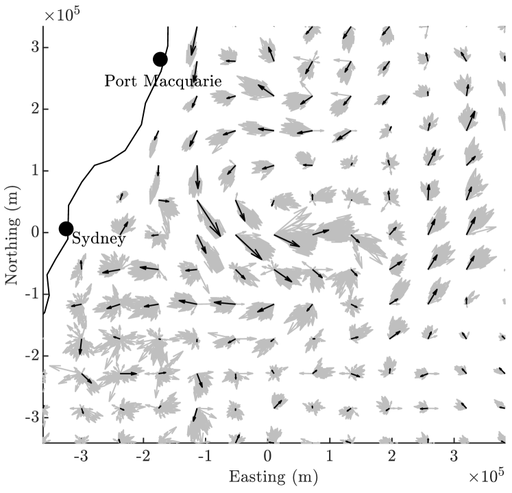
Figure 1: Subsampled ensemble flow field data from the Australian Bureau of Meteorology (BOM) off the coast of New South Wales, Australia. This ensemble forecast consists of ${N_{E}=96}$ flow fields, each predicting ocean surface conditions for 16${}^{\text{th}}$ November 2018. One of the 96 flow fields is shown in black, whilst others are shown in grey.

The ensemble format is awkward for robotics applications because planning algorithms typically assume a single probabilistic environment model, as opposed to a set of predictions [1, 2]. Ensemble forecasting models flow fields by incorporating information including temperature, salinity, and the application of Navier-Stokes equations. The challenge in producing a single model is how to distil the information contained in the ensemble in a way that captures uncertainty and that preserves spatial correlations seen in the ensemble data.

In this paper, we present a novel estimation method that produces a single probabilistic model using kernel methods and singular value decomposition (SVD). Intuitively, we find a set of basis flow fields and identify a compressed model, represented as a linear combination of these basis flows, that enforces spatial correlations found in the ensemble data. This compact representation is key to achieving computational efficiency. Then, we use a recursive Bayesian estimator to efficiently integrate online measurements.

We present the details of our method in the case of two-dimensional, time-invariant flows and provide computational analysis. Performance comparisons with the incompressible Gaussian process (GP) and kernel observer methods highlight the computational advantages of our method empirically. Further, we demonstrate the behaviour of our method using ensemble data from the Australian BOM. The results of this experiment suggest applications of our method in an active perception context where measurement locations are intentionally chosen to reduce model uncertainty.

II Related work

The problem of oceanic flow field estimation is certainly not new. Indeed, while an ensemble forecast is considered an input to our problem, the ensemble forecast itself (e.g. [3, 4]) is used to aid human meteorological forecasters in estimating atmospheric and oceanic conditions. Since an ensemble comprises many estimates, the use of filters has been previously proposed to give a single estimate of the most likely flow field. The ensemble Kalman filter [5, 6] is an extension of the celebrated Kalman filter [7] which uses the sample covariance of ensemble forecasts; additionally, particle filtering methods which do not depend on Gaussian assumptions have also been proposed for use with ensembles [8, 9]. However, direct implementation of these filters often requires copious amounts of computation power, due to their high dimensionality.

Another tool used for oceanic flow field estimation is the Gaussian process (GP), also known as “kriging”. A special GP formulation for oceanic flow field estimation has been proposed that imposes an incompressibility constraint, giving it faster convergence compared to a standard radial basis function kernel [10]. A closely related class of approaches is the kernel observer [11, 12, 13], which constructs an observer on the latent state of a kernel model. The use of these methods on an ensemble forecast has not been studied, however; typically kernel observers make use of a single dataset. Our method can be considered an extension of the kernel observer method which makes use of ensemble forecasts as a valuable prior, resulting in a lower-dimensional latent state and faster convergence rates.

Another related family of methods is based on the dynamic mode decomposition (DMD), which also has not been applied for ensemble data. DMD-based methods also seek to obtain a low-dimensional latent state with linear dynamics, and have been used successfully to represent dynamics of periodic fluid flows (e.g. [14]). Furthermore, the use of an observer on the “DMD latent state” has been investigated for fluid flow estimation [15, 16], and other time-series data [17], but not ensemble data. Our approach extends upon “DMD observer” idea by using a kernel embedding to enforce incompressibility, which is a common model for ocean currents (e.g. [18, 19]), and has been shown to improve error and convergence rate of a GP in real-world 2D oceanic flow fields [10].

In summary, the approach proposed in this paper can be seen as a novel combination of kernel methods, the SVD, and an observer for use with ensemble forecasts. It can be seen as a unification of the kernel observer with the “DMD observer”. Additionally, the proposed method leverages an ensemble forecast as a prior, leading to fast convergence to accurate estimates compared to these existing methods.

III Problem formulation and approach

We consider time-invariant ensemble forecasts on a compact subset of two-dimensional space $\mathds{R}^{2}$. An ensemble forecast $\mathscr{E}$, common in meteorological weather prediction, is a set of $N_{E}$ ensemble members ${\mathscr{e}_{i}\in\mathscr{E}}$. Each of the ensemble members $\mathscr{e}_{i}$ is deterministically generated using slightly different initial conditions which result in different sets of flow vectors, representing multiple predictions of the ocean current velocities at a discrete set of $N_{V}$ locations ${\mathscr{X}_{\text{ens}}\subset\mathds{R}^{2}}$. Each ensemble member is such that $\mathscr{e}_{i}=\{\mathbf{z}_{i,1},\cdots,\mathbf{z}_{i,N_{V}}\}$ where ${\mathbf{z}_{i,j}=[u_{i,j},v_{i,j}]^{\top}}$ is a flow vector for $i$-th ensemble member at position ${\mathbf{x}_{j}\in\mathscr{X}_{\text{ens}}}$.

A set of $N_{K}$ measurements, denoted as $\mathscr{Z}$, is taken at a set of positions $\mathscr{X}_{\text{mea}}$. While the positions are fully-known, each measurement $\tilde{\mathbf{z}}_{k}\in\mathscr{Z}$ at $\mathbf{x}_{k}\in\mathscr{X}_{\text{mea}}$ is subject to Gaussian noise, such that

$$\tilde{\mathbf{z}}_{k}=\mathbf{f}_{\text{tru}}(\mathbf{x}_{k})+\mathbf{n}_{k},$$ (1)

where $\mathbf{f}_{\text{tru}}:\mathds{R}^{2}\to\mathds{R}^{2}$ is the true, continuous, unknown flow field and ${\mathbf{n}_{k}\sim\mathcal{N}(\mathbf{0}_{2},\boldsymbol{\Sigma}_{\text{mea}}})$ is the i.i.d. measurement error with covariance $\boldsymbol{\Sigma}_{\text{mea}}\in\mathds{R}^{2\times 2}$.

We aim to estimate the continuous flow field ${\hat{\mathbf{f}}:\mathds{R}^{2}\to\mathds{R}^{2}}$ given the ensemble forecast $\mathcal{E}$ and a set of measurements $\mathscr{Z}$.

Problem 1.

Given a finite set of $N_{K}$ noisy measurements $\tilde{\mathbf{z}}_{k}\in\mathscr{Z}$, at locations $\mathbf{x}_{k}$, find a continuous flow field $\hat{\mathbf{f}}$ that minimises

$$\hat{\mathbf{f}}^{*}=\operatorname*{arg\,min}_{\hat{\mathbf{f}}\in C^{\infty}(\mathbf{x})}\sum_{k=1}^{N_{K}}\left\|\tilde{\mathbf{z}}_{k}-\hat{\mathbf{f}}(\mathbf{x}_{k})\right\|_{2}^{2}.$$ (2)

However, (2) is severely underdetermined; additional properties must be imposed to constrain the problem. The main desirable property of $\boldsymbol{\mathbf{f}}^{*}$ is to preserve spatial correlation (i.e. flow patterns) within the ensemble $\mathscr{E}$.

III-A Approach overview

Our proposed approach solves Prob. 1 with the property that $\hat{\mathbf{f}}^{*}$ preserves the spatial correlations in $\mathscr{E}$. To do this, we propose to construct $\hat{\mathbf{f}}^{*}(\mathbf{x})$ using a basis ${\boldsymbol{H}:\mathds{R}^{2}\to\mathds{R}^{2\times N_{W}}}$ and weight vector ${\mathbf{w}\in\mathds{R}^{N_{W}}}$:

$$\hat{\mathbf{f}}^{*}(\mathbf{x})=\boldsymbol{H}(\mathbf{x})\mathbf{w},$$ (3)

where $\mathbf{x}=[x,y]^{\top}$ is a location.

Our approach is to choose $\boldsymbol{H}(\mathbf{x})$ based on the ensemble data $\mathscr{E}$, and to choose $\mathbf{w}$ based on online measurements $\mathscr{Z}$. Choosing $\boldsymbol{H}(\mathbf{x})$ in this way ensures that the “flow patterns” (i.e. spatial correlations) of the resulting $\hat{\mathbf{f}}$ are consistent with the ensemble data $\mathscr{E}$. Additionally, this constrains the valid solutions to be in the span of $\boldsymbol{H}(\mathbf{x})$, excluding many spurious solutions allowed by (2), and hence aiding the ill-posedness of the problem.

We propose a two-stage estimation framework consisting of offline and online components. In our approach, since $\boldsymbol{H}(\mathbf{x})$ does not depend on $\mathscr{Z}$, it can be computed offline. The basis $\boldsymbol{H}(\mathbf{x})$ is chosen based on the ensemble forecast $\mathscr{E}$ and an additional incompressibility prior. The online component uses a recursive filter to iteratively update $\mathbf{w}$ since the measurements are often sequential.

IV Flow field representation

In this section, we describe the offline part of the proposed algorithm, comprising two steps: “regression” and “compression”. Firstly, we model each of the $N_{E}$ ensemble members resulting in continuous and incompressible representations of the ensemble flow fields encoded in latent states. Then, we extract the flow patterns from $\mathscr{E}$ with the SVD to construct a basis $\boldsymbol{H}(\mathbf{x})$ that preserves spatial correlations in $\mathscr{E}$.

IV-A Flow field regression via kernel embedding

Existing work [12, 13, 10] have successfully used kernel functions to represent flow fields in the past. The incompressible kernel [10] has recently been shown to be an apt description of smoothness and incompressibility of physical 2D flow fields. The incompressible kernel ${\boldsymbol{K}:\mathds{R}^{2}\times\mathds{R}^{2}\to\mathds{R}^{2\times 2}}$ can be expressed as

$$\boldsymbol{K}(\mathbf{x},\mathbf{x}^{\prime})=\mathbf{\mathcal{D}}(\mathbf{x})k(\mathbf{x},\mathbf{x}^{\prime})\mathbf{\mathcal{D}}\left(\mathbf{x^{\prime}}\right)^{\top},$$ (4)

where $\mathbf{\mathcal{D}}(\mathbf{x})=\begin{bmatrix}\frac{\partial}{\partial y}&-\frac{\partial}{\partial x}\end{bmatrix}^{\top}$, and ${k:\mathds{R}^{2}\times\mathds{R}^{2}\to\mathds{R}}$ is an “inner” kernel function describing how the flow vectors are expected to be given their proximity. Given prior knowledge of the underlying function, an appropriate inner kernel function can be chosen, which can lead to more accurate modelling and better convergence properties.

The Gram matrix $\boldsymbol{K}(\boldsymbol{X},\boldsymbol{X}^{\prime})$ is defined with $N_{P}$ positions $\mathbf{x}_{i}$ as columns of $\boldsymbol{X}\in\mathds{R}^{2\times N_{P}}$ and $N_{Q}$ positions $\mathbf{x}^{\prime}_{j}$ as columns of $\boldsymbol{X}^{\prime}\in\mathds{R}^{2\times N_{Q}}$:

$$\boldsymbol{K}(\boldsymbol{X},\boldsymbol{X}^{\prime})=\left[\boldsymbol{K}_{i,j}\right]\in\mathds{R}^{2N_{Q}\times 2N_{P}},$$ (5)

where $\boldsymbol{K}_{i,j}=\boldsymbol{K}(\mathbf{x}_{i},\mathbf{x}^{\prime}_{j})$. Then, given ensemble data positions $\boldsymbol{X}_{\text{ens}}=[\mathbf{x}_{1},\cdots,\mathbf{x}_{N_{V}}]$ and any spatial location ${\mathbf{x}\in\mathds{R}^{2}}$, the latent state vector $\beta\in\mathds{R}^{2N_{V}}$ encodes the flow vector $\hat{\mathbf{f}}(\mathbf{x})$ at $\mathbf{x}$ via

$$\hat{\mathbf{f}}(\mathbf{x})=\boldsymbol{K}(\mathbf{x},\boldsymbol{X}_{\text{ens}})\mathbf{\beta}.$$ (6)

For fixed $\beta$, evaluating all $\mathbf{x}\in\mathds{R}^{2}$ using (6) results in a continuous 2D flow field $\hat{\mathbf{f}}(\mathbf{x})$ that is incompressible. Then, for each ensemble member $\mathscr{e}_{i}\in\mathscr{E}$, the latent state $\beta_{i}$ is chosen by

$$\beta_{i}=\operatorname*{arg\,min}_{\mathbf{\beta}}\left\|\mathbf{\eta}_{i}-\boldsymbol{K}(\boldsymbol{X}_{\text{ens}},\boldsymbol{X}_{\text{ens}})\mathbf{\beta}\right\|_{2}^{2},$$ (7)

where $\mathbf{\eta}_{i}$ is the vectorised form of ensemble member $\mathscr{e}_{i}$, such that ${\mathbf{\eta}_{i}=[u_{i,1},v_{i,1},\cdots,u_{i,N_{V}},v_{i,N_{V}}]^{\top}}$.

In our approach, the estimated flow field is refined by adjusting values in the latent state representation. Our choice of the kernel function $\boldsymbol{K}$ ensures that the resulting flow field is always incompressible.

IV-B Model compression by SVD

In (6), $\boldsymbol{K}$ could be considered a candidate $\boldsymbol{H}(\mathbf{x})$. However, it would not preserve the spatial correlations in $\mathscr{E}$. This subsection addresses the construction of a $\boldsymbol{H}(\mathbf{x})$ so that the spatial correlations are preserved via the SVD. This admits a lower-dimensional representation of $\hat{\mathbf{f}}$ by additionally constraining $\hat{\mathbf{f}}$ at $\mathscr{X}_{\text{ens}}$ to be in the span of $\mathscr{E}$, hence the name “compression”.

First, the latent states of the ensemble members are concatenated for the latent matrix $\boldsymbol{B}\in\mathds{R}^{2N_{V}\times N_{E}}$

$$\boldsymbol{B}=\begin{bmatrix}\mathbf{\beta}_{1}&\mathbf{\beta}_{2}&\cdots&\mathbf{\beta}_{N_{E}}\end{bmatrix}.$$ (8)

Then the thin SVD provides the compact representation:

$$\boldsymbol{B}=\boldsymbol{U}\boldsymbol{\Sigma}\boldsymbol{V}^{H},$$ (9)

where $(\cdot)^{H}$ is the conjugate transpose operator. Since the number of ensembles is typically much less than that of the variables in the latent state ($N_{E}\ll 2N_{V}$), the left-singular vector ${\boldsymbol{U}\in\mathds{R}^{2N_{V}\times N_{E}}}$ is rectangular whilst the right-singular vector ${\boldsymbol{V}\in\mathds{R}^{N_{E}\times N_{E}}}$ and the diagonal matrix ${\boldsymbol{\Sigma}\in\mathds{R}^{N_{E}\times N_{E}}}$ of singular values $\sigma_{i}$ are square.

The columns of $\boldsymbol{U}$ are referred to as the latent state components $\mathbf{u}_{i}$, and corresponds to the latent states of the basis flow fields. The singular values $\sigma_{i}$ can be interpreted as the significance of the basis flow fields in the ensemble. The columns of $\boldsymbol{V}$ describe the relative contribution of basis flow fields for the corresponding ensemble flow field.

The weight matrix $\boldsymbol{W}\in\mathds{R}^{N_{E}\times N_{E}}$ is defined as

$$\boldsymbol{W}=\boldsymbol{\Sigma}\boldsymbol{V}^{H},$$ (10)

the columns of which are weight vectors $\mathbf{w}_{i}\in\mathds{R}^{N_{E}}$. The basis $\boldsymbol{H}$ can now be defined as

$$\boldsymbol{H}(\mathbf{x})=\boldsymbol{K}(\mathbf{x},\boldsymbol{X}_{\text{ens}})\boldsymbol{U}.$$ (11)

The basis flow fields can be visualised by plotting $\boldsymbol{H}(\mathbf{x})$ using only one latent state component $\mathbf{u}_{i}$ instead of $\boldsymbol{U}$. Figure 2 shows an example of model compression process using an ensemble consisting of flow fields similar to the one shown in Fig. 2(a). The ensemble data example can largely be represented with the three basis flow fields (Fig. 22(c)-2(e)), with the three largest singular values.

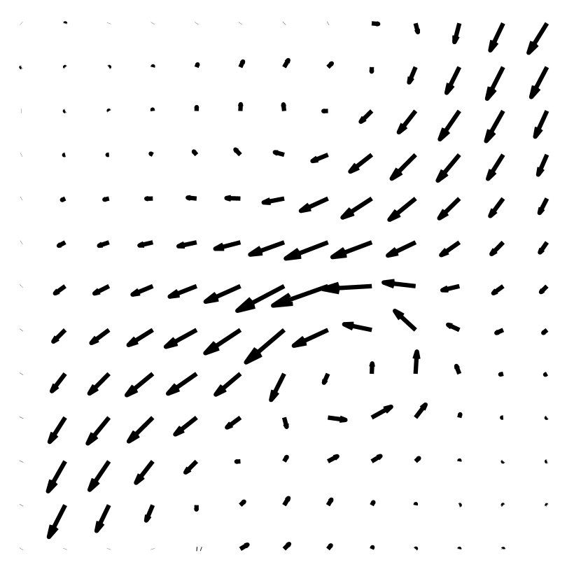
(a) Ensemble member $\mathbf{\eta}_{1}$

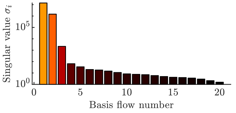
(b) Basis flow singular values

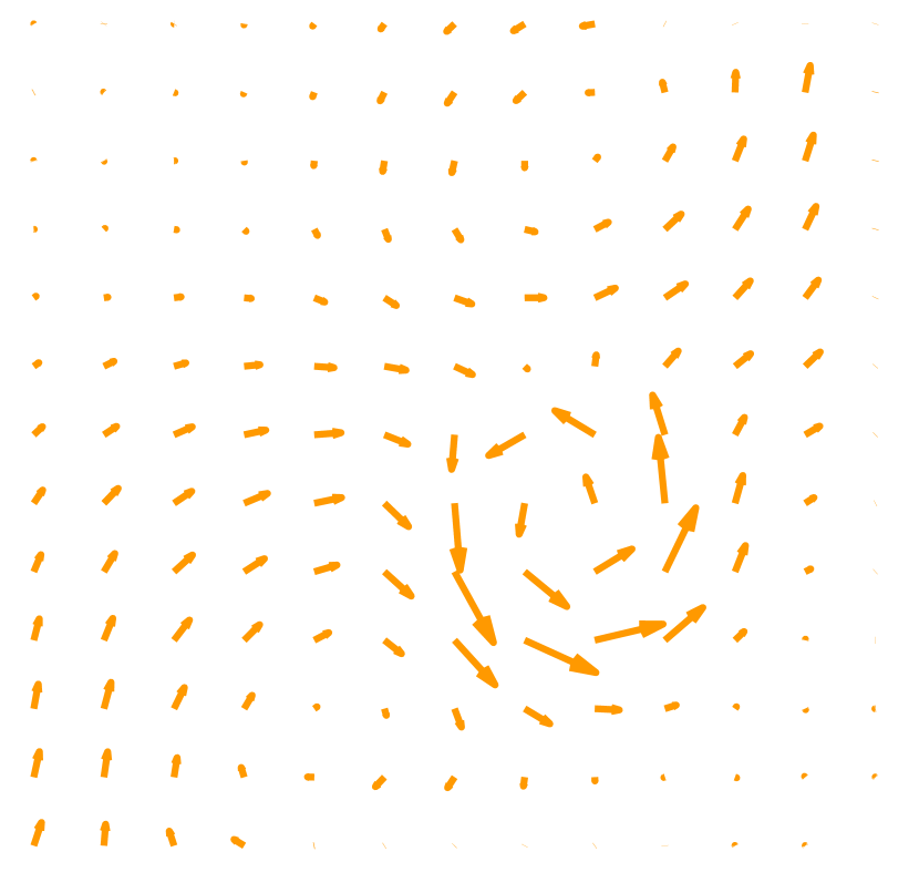
(c) $\boldsymbol{K}(\boldsymbol{X}_{\text{ens}},\boldsymbol{X}_{\text{ens}})\mathbf{u}_{1}$

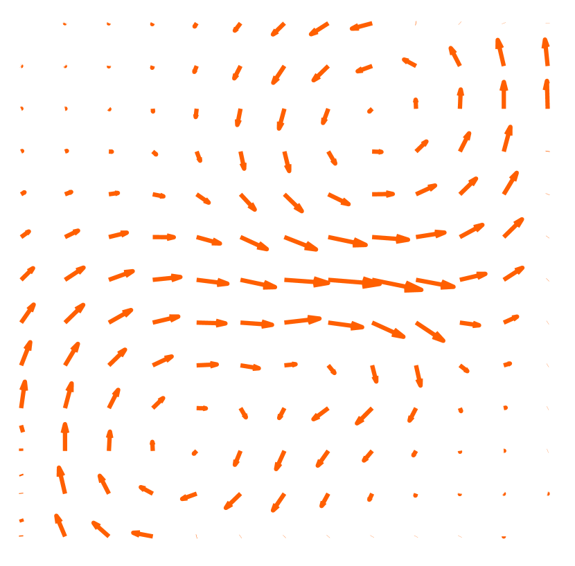
(d) $\boldsymbol{K}(\boldsymbol{X}_{\text{ens}},\boldsymbol{X}_{\text{ens}})\mathbf{u}_{2}$

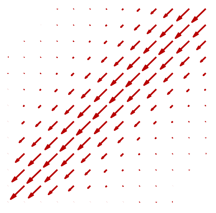
(e) $\boldsymbol{K}(\boldsymbol{X}_{\text{ens}},\boldsymbol{X}_{\text{ens}})\mathbf{u}_{3}$

Figure 2: Model compression for ensemble flow field models. (2(b)) shows the singular values in descending order. (2(c)-2(e)) shows the three most significant basis flow fields which can be used to reconstruct the flow field in (2(a)).

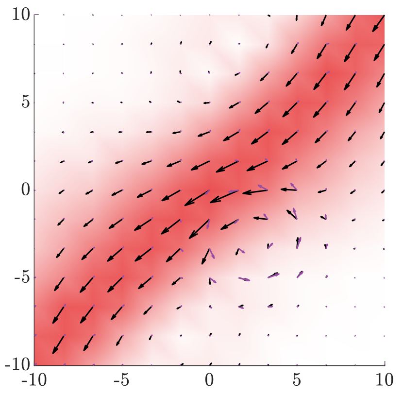
(a) $k=0$

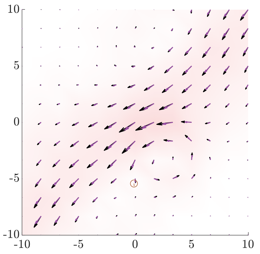
(b) $k=1$

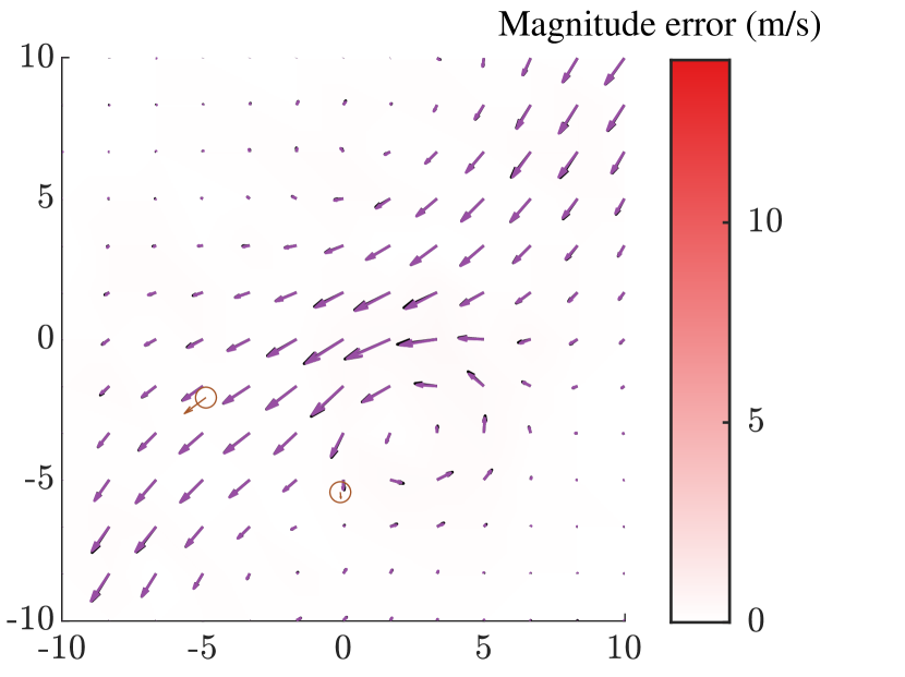
(c) $k=2$

Figure 3: Estimated flow fields after $k$ measurements. The estimated flow field (purple) quickly converges to the true flow field (black) after a few measurements. The red heatmap shows the magnitude flow field error across space. Measurements are shown as circled brown arrows.

We can choose to represent the flow field with $N_{W}\leq N_{E}$ weights by keeping only the highest $N_{W}$ singular values of the SVD and the corresponding columns of $\boldsymbol{U}$ and $\boldsymbol{V}$. In particular, choosing $N_{W}<N_{E}$ effectively ignores the effects of basis flow fields that vary less in the ensemble.

V Online flow field estimation

In the previous section, we described the offline stage of our approach, representing a flow field as a weight vector $\mathbf{w}$ with each weight corresponding to the basis flow fields of the ensemble data. In this section, we propose a process to incorporate information from noisy online measurements to improve estimation accuracy by recursively updating $\mathbf{w}$ given an initial estimate of the flow field.

Despite being static in this paper, we model the true flow field as a degenerate discrete-time linear dynamical system, which can easily be extended for use in the time-varying case. The process and measurement models of the true flow field are

$$\mathbf{w}_{k} =\boldsymbol{A}\mathbf{w}_{k-1}$$ (12)

$$\mathbf{z}_{k} =\boldsymbol{H}(\mathbf{x}_{k})\mathbf{w}_{k}+\mathbf{n}_{k},$$ (13)

where $\boldsymbol{A}=\boldsymbol{I}_{N_{W}\times N_{W}}$ is the state transition model for the static flow field, and ${\mathbf{n}_{k}\sim\mathcal{N}(\mathbf{0}_{2\times 1},\boldsymbol{\Sigma}_{\text{mea}})}$ is the i.i.d. measurement error with covariance $\boldsymbol{\Sigma}_{\text{mea}}$. The Kalman filter [7] is employed as it is the optimal estimator for measurements with Gaussian noise [20]; the Kalman filter equations are well-known (e.g. [21]) and are omitted for brevity.

As a recursive estimator, the Kalman filter needs to be initialised with some estimate. The columns of the weight matrix $\boldsymbol{W}$ are the weight vectors that correspond to each ensemble flow field, so an estimate can be obtained by aggregating them. An initial estimate weight vector $\hat{\mathbf{w}}_{0}$ and its covariance ${\boldsymbol{P}_{0}\in\mathds{R}^{N_{W}\times N_{W}}}$ is defined as the row-wise mean and the diagonal matrix of row-wise variances of the weight matrix $\boldsymbol{W}$.

Figure 3 shows an example of the estimated flow fields after $k$ measurements. The rapid convergence to the true flow field can be attributed to a good initial estimate from the ensemble data, and well-placed measurements.

VI Analysis

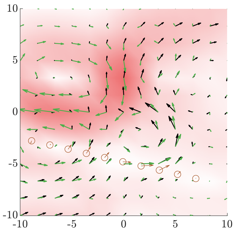
(a) Kernel observer [12] estimate

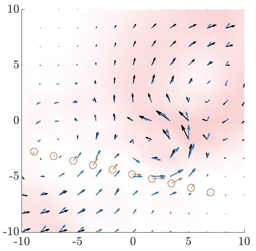
(b) Incompressible GP [10] estimate

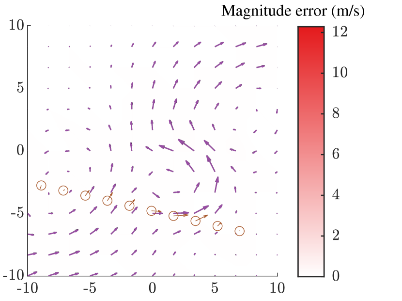
(c) Our approach

Figure 4: Comparison of flow field estimation using equally-spaced measurements (circled brown arrows) from the bottom right to the left. The magnitude error between the estimated and the true flow field (black) is shown as a red heatmap.

Assuming that the environment is large, the number of ensemble positions $N_{V}$ is greater than the number of ensemble members in $\mathscr{E}$ (i.e. $N_{E}\ll N_{V}$). Under this assumption, we demonstrate the worst-case computation time complexity in Table I for our framework as well as for kernel observer (KO) [12], Gaussian process (GP) [10], and least squares regression (LS) methods.

TABLE I: Computational complexity of compared approaches

	Initialise	Update	Query
KO	$\mathcal{O}\left(N_{V}^{3}\right)$	$\mathcal{O}\left(N_{V}^{3}\right)$	$\mathcal{O}\left(N_{V}\right)$
GP	$\mathcal{O}\left(N_{V}\right)$	$\mathcal{O}\left(1\right)$	$\mathcal{O}\left((N_{K}+N_{V})^{3}\right)$
LS	$\mathcal{O}\left(N_{V}^{3}\right)$	$\mathcal{O}\left(N_{W}^{3}+N_{K}N_{W}^{2}\right)$	$\mathcal{O}\left(N_{V}N_{W}\right)$
Ours	$\mathcal{O}\left(N_{V}^{3}\right)$	$\mathcal{O}\left(N_{W}^{3}+N_{V}N_{W}\right)$	$\mathcal{O}\left(N_{V}N_{W}\right)$

The kernel observer approach is proposed to estimate a time-varying latent state with very few measurements. For comparison, in the time-invariant case with ensembles, we adapt the framework by setting the transition operator to the identity, and initialising its estimate with the ensemble latent states. This adaptation is identical to our approach up to forming the latent matrix in (8), after which the mean and variance of $\boldsymbol{B}$ is used to initialise their Kalman filter. The GP approach utilises a kernel that allows for an estimate of incompressible flow fields from flow vector measurements and is adapted for use with ensembles by finding the set of flow vector mean and covariances over individual ensemble positions $\mathscr{X}_{\text{ens}}$, which is then added as prior flow field measurements. Whilst the Kalman filter shares the same estimation performance as least squares, a least squares variation of our approach is included to highlight the computational disadvantages in the context of our problem. A useful aspect of the least squares approach is that it does not need to be initialised with an estimate. Note that all the listed approaches generate incompressible flow fields through the use of the incompressible kernel [10].

In Table I, we have time complexities for three operations: 1) initialise (with ensemble forecast), 2) update where the estimate $\hat{\mathbf{f}}$ is updated with a single measurement, and 3) query where a flow vector estimate is queried at an arbitrary position. The complexities are described with the number of ensemble positions $N_{V}$, the number of weights $N_{W}$, and the number of accumulated measurements $N_{K}$.

For those methods with similar steps to our method (i.e. KO, LS), the time complexity is $\mathcal{O}\left(N_{V}^{3}\right)$, whereas that for the GP is $\mathcal{O}\left(N_{V}\right)$. This is because the GP computes the flow field lazily, and just stores the $N_{V}$ aggregated flow vectors from the ensemble. Ours computes the latent representation of each ensemble flow field for basis flow field extraction. The basis flow fields captures the spatial correlations of flow vectors in the ensemble data. Unlike our method, the GP loses significant amount of information since it is unable to capture this spatial correlation.

The complexity for update is also similar among the KO, LS and our method with two important differences. Our method reduces the number of estimated variables by compressing a representation with $\mathbf{\beta}$ to the low-dimensional representation $\mathbf{w}$, unlike the KO approach where compression is omitted. Since $N_{W}\leq N_{E}\ll N_{V}$, ours outperforms the KO even without truncation (i.e. when $N_{W}=N_{E}$). For the LS method, one particular implementation is to update the weight vector after each measurement, which requires all $N_{K}$ measurements to be considered. This particular implementation becomes intractable as the number of past measurements grows large over time. For the GP, the update is performed by concatenating the new measurement to the existing set.

For querying a position, the GP method requires an inversion of the Gram matrix (5) between the positions of the collected measurements and itself. This is an expensive operation that is cubic in complexity [22], so as the number of measurements becomes large, the time complexity approaches $\mathcal{O}\left(N_{K}^{3}\right)$.

As a whole, our method directly exploits the incompressible basis flow fields present in the ensemble members to fit the weights to the measurements. The compact representation of flow fields as weights significantly reduce the time complexities for update and query operations with compression and truncation. We show that these operations are not dependent on the number of past measurements. This is an important property, especially in long-term missions and closed-loop path planning where a robot continuously measures the flow field to update its estimate.

VII Empirical results

In this section, we compare the performance of our method against existing approaches. We show that our method reduces the estimation error across the environment while the existing approaches are limited to the neighbourhood of measurements. We also empirically validate the theoretical properties for update and query time. Then, we use real ensemble forecast provided by the BOM to discuss how different measurement policies affect the accuracy of flow estimation. We argue how our method could be implemented for various planning problems, especially active perception [23, 24, 25], where regular updates with measurements is necessary. In all demonstrations, we use the incompressible kernel in (4) with the squared exponential kernel [22]:

$$k(\mathbf{x},\mathbf{x}^{\prime})=k_{\text{SE}}(\mathbf{x},\mathbf{x}^{\prime})=\sigma_{\text{ker}}^{2}\exp{\left(\frac{\left\|\mathbf{x}^{\prime}-\mathbf{x}\right\|_{2}^{2}}{2\ell^{2}}\right)},$$ (14)

where $\ell$ and $\sigma_{\text{ker}}$ are hyperparameters to be tuned to the flow field of interest.

VII-A Estimation comparison with existing approaches

We compare our method against the incompressible GP (GP) [10], an adaptation of the kernel observer [12] with Kalman filter (KO), and the least squares implementation of our method (LS). We synthetically construct an ensemble of $N_{E}=20$ flow fields over $N_{V}=169$ positions, shown in Fig. 4. The true flow field $\mathbf{f}_{\text{tru}}$ is shown with black arrows. Starting at $\mathbf{x}=[6.98,-6.42]^{\top}$, the vehicle makes a set of $10$ measurements with noise ${\boldsymbol{\Sigma}_{\text{mea}}=10^{-3}\boldsymbol{I}_{2\times 2}}$ that are $2$ $\mathrm{m}$ apart while moving in a straight line. The measurement positions are shown with brown circles with measurement vectors as arrows.

In Fig. 4(a), the flow field estimate from KO is shown. The KO method utilises the latent state of the kernel $\mathbf{\beta}$ with the size of $338$ (i.e. $2N_{V}$). We observe large errors; we suspect that due to the large latent state, the problem is still underdetermined.

In Fig. 4(b), we show the estimates using incompressible GP [10] over the synthetic ensemble data. The estimation after the measurements is shown with blue arrows and the error magnitude is shown in red. As discussed in Sec. VI, the GP method is unable to make use of all the spatial correlations present in the ensemble resulting in lower sampling efficiency. As a consequence, the error is only reduced in the neighbourhood of measurements while the distant regions are virtually not affected.

The estimates from our method are shown in Fig. 4(c). Using our method, decomposition in Sec. IV found three representative basis flow fields. As a consequence, the number of basis flows can be reduced from $20$ (i.e. $N_{E}$) to $3$ (i.e. $N_{W}$) after truncation with virtually no degradation in estimation performance. We show that our method significantly reduces distant errors, unlike the GP and KO methods. Unlike the KO method, the number of unknown variables in our approach is also much smaller (i.e. $N_{W}\ll 2N_{V}$) so less measurements are required to properly determine the variables. The results also show that the distant positions from measurements are well estimated since our method considers spatial correlations in flow fields unlike the GP method.

In Fig. 5, we show how our method scales in the number of past measurements $N_{K}$. As claimed in Sec. VI, the update time shown in Fig. 5(a) stays almost constant in the number of measurements except the LS method. It is important to note that the update time for our method is much lower than the KO due to our compressed representation (i.e. $N_{W}\ll 2N_{V}$). Likewise, the query time shown in Fig. 5(b) stays constant for our method while it increases for the GP method which is shown to be $\mathcal{O}\left(N_{K}^{3}\right)$ in Sec. VI. Overall, the empirical comparison shows that our method scales in a suitable way for applications that take a large number of measurements.

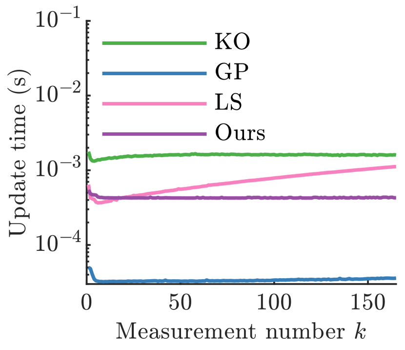
(a) Iteration time per measurement

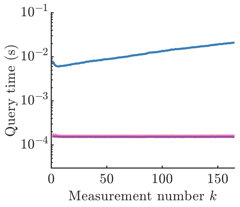
(b) Query time per position

Figure 5: Comparison of mean computational times between the kernel observer (KO) [12], incompressible Gaussian process (GP) [10], a least squares (LS) implementation of our approach, and our approach on the flow field shown in Fig. 4. Values are averaged over $1000$ trials, the $99.73\%$ confidence intervals of which are virtually imperceptible, and are omitted.

VII-B Measurement policies in real ensemble flow fields

We show how different measurement policies affect the estimation performance using our method. We use the ensemble forecast data provided by the BOM where a portion of the data is shown in Fig. 1. We compare three policies: uniform where measurement positions are randomly taken, subspace where measurements are only taken within a subsection with high uncertainty, and active where measurements are taken at positions with flow vector high uncertainty.

In Fig. 6, we show the root mean square (RMS) error with increasing number of past measurements. For reference, we have the ideal condition where measurements are taken exactly at ensemble positions $\mathscr{X}_{\text{ens}}$ such that the the final error after all measurements is shown with dashed orange line. Since ground-truth is not known for this forecast data, the error for each policy is evaluated using leave-one-out cross-validation (LOOCV) [26], where we initialise the estimates without one chosen ensemble member and compare the estimates against that chosen member. We then compute the RMS of the residuals at $\mathscr{X}_{\text{ens}}$. For each measurement policy, a trial is performed once with a fixed random seed. The RMS error is shown in coloured lines and its $3\sigma$ confidence interval is shown as a shaded band.

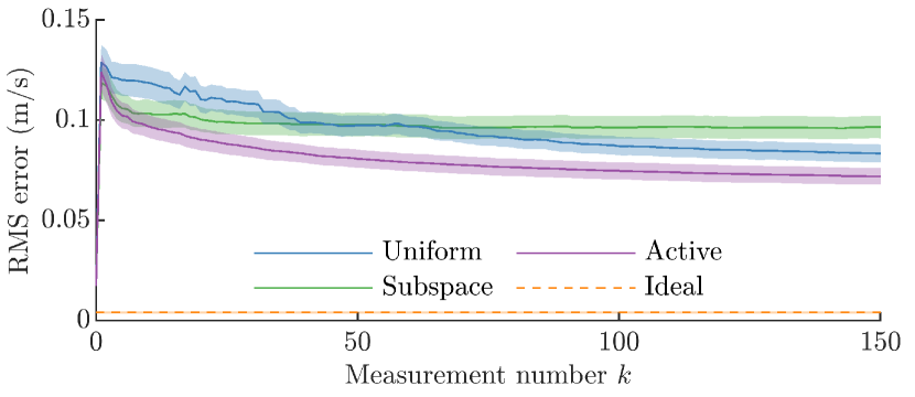
Figure 6: Root mean square (RMS) error from flow field estimation using different measurement policies using our approach. The flow field is based on the real ensemble data shown in Fig. 1. The $99.73\%$ confidence intervals for these errors are shown for each measurement policy.

The results show that the active policy outperforms all other policies. It is interesting to observe that the convergence rate to the ideal is much faster using our approach. The uniform policy initially underperforms compared to the subspace because the subspace policy focuses the measurements in a region with high uncertainty so its reduction in error is larger. However, as the number of measurements increases, the uniform policy starts to outperform the subspace policy. This is because the subspace policy is constrained to a small region whereas the uniform policy takes measurements across the environment.

The policy comparison result indicates that existing path planning approaches will benefit from our method in that a carefully-chosen measurement policy will greatly affect the quality of the estimated flow field which will in turn affect the quality of the planned path. For example, we can formulate an active perception problem that involves finding a set of unknown features over uncertain ocean currents. Unlike the traditional problems, we do not simply maximise our information over the features but also over ocean currents since practical ocean vehicles are typically advected by ocean currents [27, 28, 1]. Our method is both theoretically and empirically validated for use in such a problem setting.

VIII Conclusion and future work

In this paper we have presented a novel algorithm for ocean flow field estimation. By leveraging ensemble data as a prior and integrating sequential online measurements, fast convergence to a good estimate is achieved in synthetic and real-world conditions.

One limitation is the assumption of time-invariant flows, but ensemble data is available over large time windows. Blending dynamic mode decomposition (DMD) approaches for the corresponding approximate linear dynamical system could draw out the full potential of our method in the time-varying case. An interesting immediate application is to exploit the spatially-correlated probabilistic representation of the flow field in path planning [29, 30, 31, 32, 33, 34] in uncertain flows.

References

- [1] T. Wang, O. P. Le Maître, I. Hoteit, and O. M. Knio, “Path planning in uncertain flow fields using ensemble method,” Ocean Dyn., vol. 66, no. 10, pp. 1231–1251, 2016.
- [2] D. Kularatne, H. Hajieghrary, and M. A. Hsieh, “Optimal path planning in time-varying flows with forecasting uncertainties,” in Proc. of IEEE ICRA, 2018, pp. 4857–4864.
- [3] M. Leutbecher and T. N. Palmer, “Ensemble forecasting,” J. Comput. Phys., vol. 227, no. 7, pp. 3515–3539, 2008.
- [4] T. N. Krishnamurti, C. M. Kishtawal, Z. Zhang, T. LaRow, D. Bachiochi, E. Williford, S. Gadgil, and S. Surendran, “Multimodel ensemble forecasts for weather and seasonal climate,” J. Clim., vol. 13, no. 23, pp. 4196–4216, 2000.
- [5] P. L. Houtekamer and H. L. Mitchell, “A sequential ensemble Kalman filter for atmospheric data assimilation,” Mon. Weather Rev., vol. 129, no. 1, pp. 123–137, 2001.
- [6] G. Evensen, “The ensemble Kalman filter: Theoretical formulation and practical implementation,” Ocean Dyn., vol. 53, no. 4, pp. 343–367, 2003.
- [7] R. E. Kalman, “A new approach to linear filtering and prediction problems,” J. Basic Eng., vol. 82, no. 1, pp. 35–45, 1960.
- [8] H. Moradkhani, K.-L. Hsu, H. Gupta, and S. Sorooshian, “Uncertainty assessment of hydrologic model states and parameters: Sequential data assimilation using the particle filter,” Water Resour. Res., vol. 41, no. 5, 2005.
- [9] H. H. Holm, M. L. Sætra, and A. R. Brodtkorb, “Data assimilation for ocean drift trajectories using massive ensembles and GPUs,” in Finite Volumes for Complex Applications IX - Methods, Theoretical Aspects, Examples, 2020, pp. 715–723.
- [10] K. M. B. Lee, C. Yoo, B. Hollings, S. Anstee, S. Huang, and R. Fitch, “Online estimation of ocean current from sparse GPS data for underwater vehicles,” in Proc. of IEEE ICRA, 2019, pp. 3443–3449.
- [11] K. V. Mardia, C. Goodall, E. J. Redfern, and F. J. Alonso, “The kriged Kalman filter,” Test, vol. 7, no. 2, pp. 217–282, 1998.
- [12] H. A. Kingravi, H. Maske, and G. Chowdhary, “Kernel observers: Systems-theoretic modeling and inference of spatiotemporally evolving processes,” in Proc. of NIPS, 2016, pp. 3990–3998.
- [13] J. Whitman and G. Chowdhary, “Learning dynamics across similar spatiotemporally-evolving physical systems,” in Proc. of CoRL, vol. 78, 2017, pp. 472–481.
- [14] J. N. Kutz, S. L. Brunton, B. W. Brunton, and J. L. Proctor, Dynamic Mode Decomposition: Data-Driven Modeling of Complex Systems. SIAM, 2016.
- [15] J. H. Tu, J. Griffin, A. Hart, C. W. Rowley, L. N. Cattafesta, and L. S. Ukeiley, “Integration of non-time-resolved PIV and time-resolved velocity point sensors for dynamic estimation of velocity fields,” Exp. Fluids, vol. 54, no. 2, p. 1429, 2013.
- [16] T. Nonomura, H. Shibata, and R. Takaki, “Dynamic mode decomposition using a Kalman filter for parameter estimation,” AIP Adv., vol. 8, no. 10, pp. 1–27, 2018.
- [17] M. F. Fathi, A. Baghaie, A. Bakhshinejad, R. H. Sacho, and R. M. D’Souza, “Time-resolved denoising using model order reduction, dynamic mode decomposition, and kalman filter and smoother,” J. Comput. Dyn., vol. 7, no. 2, pp. 469–487, 2020.
- [18] Z. Kowalik and T. S. Murty, Numerical modeling of ocean dynamics. World Scientific, 1993, vol. 5.
- [19] G. Madec, NEMO ocean engine. Note du Pôle de modélisation, Institut Pierre-Simon Laplace (IPSL), France, No 27, 2008.
- [20] J. Humpherys, P. Redd, and J. West, “A fresh look at the kalman filter,” SIAM Rev., vol. 54, no. 4, pp. 801–823, 2012.
- [21] S. Thrun, W. Burgard, and D. Fox, Probabilistic Robotics. MIT Press, 2005.
- [22] C. E. Rasmussen and C. K. I. Williams, Gaussian Processes for Machine Learning. The MIT Press, 2006.
- [23] F. Sukkar, G. Best, C. Yoo, and R. Fitch, “Multi-robot region-of-interest reconstruction with Dec-MCTS,” in Proc. of IEEE ICRA, 2019, pp. 9101–9107.
- [24] K. M. B. Lee, J. J. H. Lee, C. Yoo, B. Hollings, and R. Fitch, “Active perception for plume source localisation with underwater gliders,” in Proc. of ARAA ACRA, 2018, pp. 1–10.
- [25] R. Bajcsy, Y. Aloimonos, and J. K. Tsotsos, “Revisiting active perception,” Auton. Robot., vol. 42, no. 2, pp. 177–196, 2018.
- [26] C. M. Bishop, Pattern Recognition and Machine Learning. Springer-Verlag New York, 2006.
- [27] T. Inanc, S. C. Shadden, and J. E. Marsden, “Optimal trajectory generation in ocean flows,” in Proc. of IEEE ACC, 2005, pp. 674–679.
- [28] B. Claus, R. Bachmayer, and C. D. Williams, “Development of an auxiliary propulsion module for an autonomous underwater glider,” Proc. Inst. Mech. Eng. M, vol. 224, no. 4, pp. 255–266, 2010.
- [29] K. Y. C. To, K. M. B. Lee, C. Yoo, S. Anstee, and R. Fitch, “Streamlines for motion planning in underwater currents,” in Proc. of IEEE ICRA, 2019, pp. 4619–4625.
- [30] K. Y. C. To, J. J. H. Lee, C. Yoo, S. Anstee, and R. Fitch, “Streamline-based control of underwater gliders in 3D environments,” in Proc. of IEEE CDC, 2019, pp. 8303–8310.
- [31] K. Y. C. To, C. Yoo, S. Anstee, and R. Fitch, “Distance and steering heuristics for streamline-based flow field planning,” in Proc. of IEEE ICRA, 2020, pp. 1867–1873.
- [32] C. Yoo, J. J. H. Lee, S. Anstee, and R. Fitch, “Path planning in uncertain ocean currents using ensemble forecasts,” in Proc. of IEEE ICRA, 2021.
- [33] C. Yoo, S. Anstee, and R. Fitch, “Stochastic path planning for autonomous underwater gliders with safety constraints,” in Proc. of IEEE/RSJ IROS, 2019, pp. 3725–3732.
- [34] G. D’urso, J. J. H. Lee, O. Pizarro, C. Yoo, and R. Fitch, “Hierarchical MCTS for scalable multi-vessel multi-float systems,” in Proc. of IEEE ICRA, 2021.