Accumulations of Projections—A Unified Framework for Random Sketches in Kernel Ridge Regression

Abstract

Building a sketch of an $n$-by-$n$ empirical kernel matrix is a common approach to accelerate the computation of many kernel methods. In this paper, we propose a unified framework of constructing sketching methods in kernel ridge regression (KRR), which views the sketching matrix $S$ as an accumulation of $m$ rescaled sub-sampling matrices with independent columns. Our framework incorporates two commonly used sketching methods, sub-sampling sketches (known as the Nyström method) and sub-Gaussian sketches, as special cases with $m=1$ and $m=\infty$ respectively. Under the new framework, we provide a unified error analysis of sketching approximation and show that our accumulation scheme improves the low accuracy of sub-sampling sketches when certain incoherence characteristic is high, and accelerates the more accurate but computationally heavier sub-Gaussian sketches. By optimally choosing the number $m$ of accumulations, we show that a best trade-off between computational efficiency and statistical accuracy can be achieved. In practice, the sketching method can be as efficiently implemented as the sub-sampling sketches, as only minor extra matrix additions are needed. Our empirical evaluations also demonstrate that the proposed method may attain the accuracy close to sub-Gaussian sketches, while is as efficient as sub-sampling-based sketches.

To appear in the 24th International Conference on Artificial Intelligence and Statistics (AISTATS 2021)

1 Introduction

Kernel methods are widely used in the machine learning community. As a powerful tool, they map data to a higher dimensional feature space and hence can be widely applied to capture nonlinear structures. A well-known representative of kernel methods is the kernel ridge regression (KRR) (Shawe-Taylor et al., 2004; Hastie et al., 2005), which leads to a closed-form estimator and a solid theoretical guarantee on the statistical performance (Stone, 1982; Kanagawa et al., 2018; Tuo et al., 2020). Despite the attractive merits, a practical drawback of KRR is the expensive computational cost. As is common in many other kernel-based machine learning algorithms, solving the KRR with massive data requires manipulating and inverting large matrices usually beyond the capacity of the memory and the time constraint. For example, the evaluation of the empirical kernel matrix $K$ takes $\Theta(n^{2})$ time, which already becomes formidable for datasets with hundreds to thousands of samples.

To overcome the limitation, some random projection methods are raised to accelerate the KRR by finding a low-rank approximation to the empirical kernel matrix $K$. Popular methods include Nyström methods (Williams and Seeger, 2001; Rudi et al., 2015), random features (Rahimi and Recht, 2008), and sketching methods (Woodruff, 2014; Yang et al., 2017; Ahle et al., 2020), the theme of our paper. Actually the sketching method is a general concept that can incorporate many other methods as special cases. One of the most famous examples is the Nyström method, which approximates $K$ by using a subset of “landmark” samples. This procedure to construct an approximation to the kernel matrix is equivalent to the usage of a sub-sampling sketching matrix under our framework. Another example is the sub-Gaussian sketching method.

Different sketching methods have their own advantages and disadvantages. A common observation is that the Nyström method with uniform sampling distribution needs more “landmark” data points to achieve the same accuracy as a sub-Gaussian sketch (Alaoui and Mahoney, 2015; Yang et al., 2017). To resolve the issue, many works propose data-dependent sampling schemes (Wang and Zhang, 2013; Gittens and Mahoney, 2013; Li et al., 2016) to select the landmarks that improve the approximation of $K$, Among those weighted sampling schemes statistical leverage-score-based approaches (Alaoui and Mahoney, 2015; Musco and Musco, 2017; Rudi et al., 2018) have attracted most attention due to their superior empirical performances and strong theoretical support. On the other hand, sub-Gaussian sketching methods, although attaining higher statistical accuracy, still suffer from a practically intractable computational cost of at least $\Theta(n^{2})$ for evaluating $K$.

To fully understand the gap in statistical performance between different sketching methods and provide a unified perspective, in this paper we propose a new framework for approximate KRR via randomized sketches. Under this framework, a sketching matrix is taken as an accumulation of $m$ re-scaled sub-sampling matrices with independent columns. The framework incorporates the Nyström method and sub-Gaussian sketches mentioned above as two special cases, by setting $m=1$ and $m=\infty$ (according to the central limit theorem) respectively. We also analyze the approximation error between the estimator obtained by a sketching method and the original KRR estimator. From the analysis, we find that both the projection dimension $d$ and the number of sub-sampling matrices $m$ contribute to the reduction of the approximation error. Concretely, $d$ addresses the intrinsic difficulty of the KRR problem and is required to be at least $\widetilde{\mathcal{O}}(d_{stat})$ (complexity modulo poly-log term), where $d_{stat}$ is the statistical dimension of the problem; while the number of non-zero elements, or the density of the sketching matrix, indicated by $m\cdot d$, helps mitigate the impact of the high incoherence of the data. More precisely, the incoherence measures the sparsity of the singular vectors of $K$, and low incoherence means that all coordinates of the singular vectors of $K$ have similar magnitudes instead of few coordinates having dominating values.

Our framework naturally motivates a new method to construct the sketching matrix. Accumulating $m$ sub-sampling matrices by optimally selecting $m$, the resulting sketching method can achieve the best of two worlds—it achieves high statistical accuracy close to sub-Gaussian sketches, and still retains the high computational efficiency compared to the Nyström methods. The following toy example in Figure 1 illustrates the performance of our method. We run the tests on several synthetic datasets generated from the same distribution while with different sample sizes. (The complete setting of this toy example can be found in the appendix.) We remark here that our method utilizes the sparsity of the sketching matrix to accelerate the training of KRR estimators, and with a medium $m$ it improves the trade-off between accuracy and efficiency.

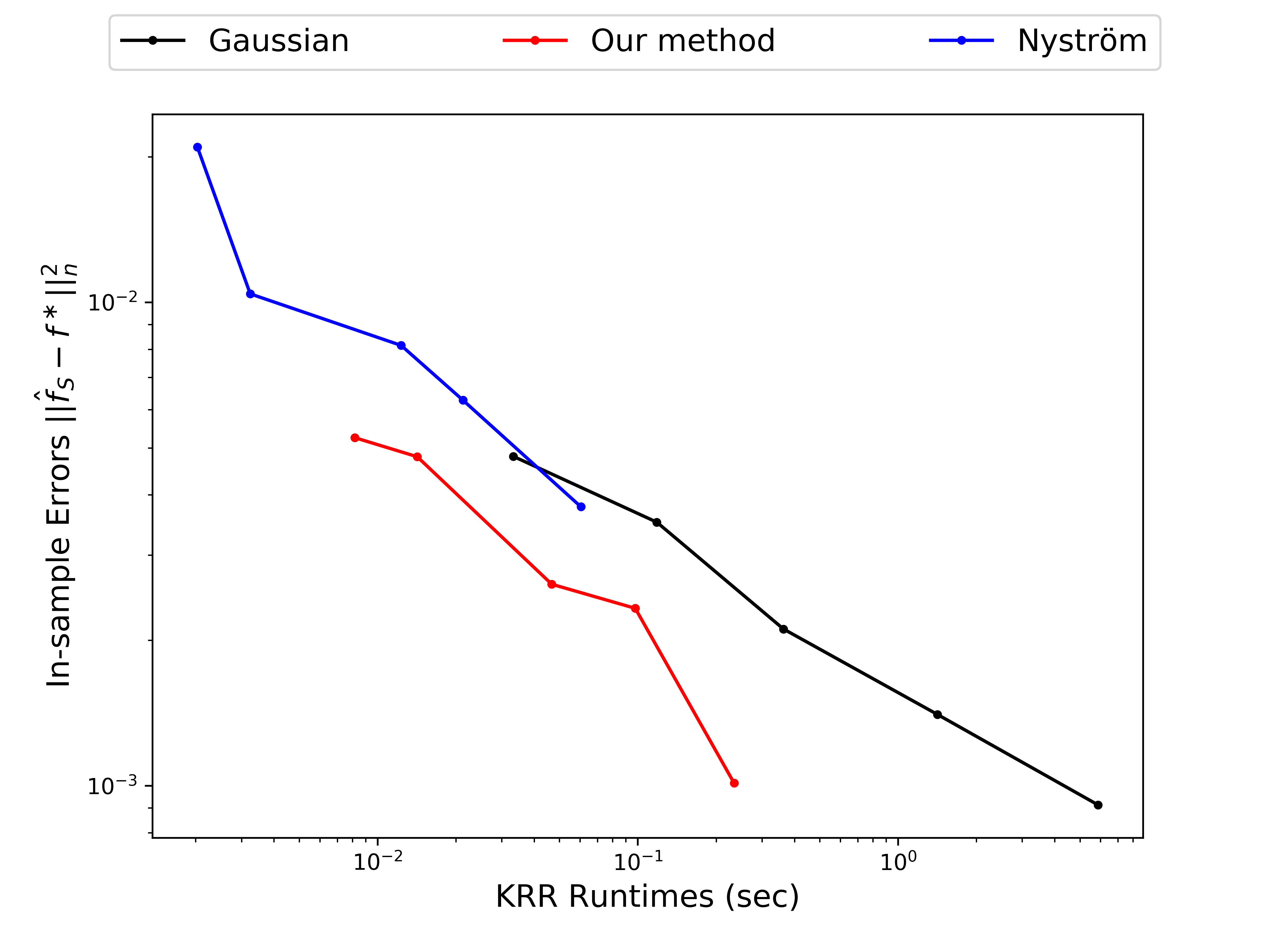
Figure 1: A Toy Example

A similar idea of utilizing sparsity has also appeared in some previous works. Localized sketching (Srinivasa et al., 2020) chooses to use a block-diagonal sketching matrix. Sparse random projections (Achlioptas, 2003; Li et al., 2006) instead randomly set some elements in the projection matrix as zero to increase sparsity. However, there are several important differences between our method and theirs. First, localized sketching assumes the data is partitioned in advance and is mainly designed for distributed or streaming settings. Second, sparse random projections require i.i.d. elements, while our method only requires i.i.d. columns of the sketching matrix—the coordinates in each column are correlated and can follow different distributions. Third, in contrast to sparse random projections, our method exploits some properties of the matrix $K(K+n\lambda I_{n})^{-1}$ rather than assume $K$ is a general matrix to be projected. As a result, our method leads to a much sparser sketching matrix than sparse random projections—their matrix density is usually $\sqrt{n}$ times greater than ours.

We also notice that our framework may motivate a broader class of sketching schemes, for example, by using $m\cdot d$ landmarks in the Nyström method, or applies a non-uniform sampling distribution (i.e. leverage-based Nyström method). Our empirical evaluations also compare and show superior performance, with another state-of-the-art variant of the Nyström method—Falkon (Rudi et al., 2017).

1.1 Our contributions

In this work, we propose a framework to unify two common and state-of-the-art random sketching methods, and explain the difference in their statistical performances. Specifically, we consider the construction of sketching matrices as the accumulation of $m$ rescaled sub-sampling matrices, which provides a unified perspective to understand how the projection dimension (or size), and the density level of the sketching matrix together influence the approximation error of randomized sketching for KRR, under situations where the incoherence of the data is high and the vanilla Nyström approach fails.

With this framework, we unify existing theoretical results on random sketches and develop a new sketching method to accelerate the training of KRR. This method can be efficiently implemented in practice. Compared to the Nyström method, only some extra parallelizable matrix additions are needed, thereby allowing efficient implementation scalable to massive data. In short, the framework allows the new method to achieve “best of both worlds”: it attains the accuracy close to sub-Gaussian sketching while retains the computational efficiency as the sub-sampling sketching.

1.2 Paper outline

The rest of the paper is arranged as follows. In Section 2, we introduce some background on KRR and sketching methods. In Section 3, we illustrate our new framework, provide some theoretical analysis on approximation error, and propose a new sketching method induced by the framework. Finally, in Section 4, we do some numerical experiments to validate our claims in the paper.

2 Preliminaries and notations

Before we present a new framework for random sketches and the related theoretical analysis, we briefly discuss some preliminaries and set up some notations in this section.

2.1 Kernel ridge regression

Consider $n$ pairs of points $\{(x_{i},y_{i})\}_{i=1}^{n}$ in $\mathcal{X}\times\mathcal{Y}$, where $\mathcal{X}\subseteq\mathbb{R}^{d_{X}}$ is the input (predictor) space and $\mathcal{Y}\subseteq\mathbb{R}$ is the response space. We assume the underlying data generating process is given by the following standard non-parametric regression model,

$$y_{i}=f^{\ast}(x_{i})+\varepsilon_{i},\quad i=1,2,\ldots,n,$$

where $f^{\ast}:\,\mathcal{X}\to\mathcal{Y}$ is the unknown true regression function, and the noises $\{\varepsilon_{i}\}_{i=1}^{n}$ are i.i.d. sub-Gaussian with mean zero and variance $\sigma^{2}$. In this paper, we follow the common regularity assumption that the true regression function $f^{\ast}\in\mathbb{H}$, where $\mathbb{H}$ is the reproducing kernel Hilbert space induced by a positive semi-definite kernel function $\mathcal{K}(\cdot,\cdot):\mathcal{X}\times\mathcal{X}\to\mathbb{R}$ specified beforehand. The true regression function $f^{\ast}$, can be estimated by the kernel ridge regression (KRR) (Shawe-Taylor et al., 2004; Hastie et al., 2005), which is cast as the following minimization problem,

$$\widehat{f}_{n}=\operatorname*{arg\,min}_{f\in\mathbb{H}}\Big{\{}\frac{1}{n}\sum_{i=1}^{n}(y_{i}-f(x_{i}))^{2}+\lambda\|f\|_{\mathbb{H}}^{2}\Big{\}}.$$ (1)

With the representer theorem, the solution to the optimization problem (1) can be obtained by solving an $n$-dimensional quadratic program (Kimeldorf and Wahba, 1971). More precisely, after defining $K$ as the $n$-by-$n$ empirical kernel matrix with $K_{ij}=\mathcal{K}(x_{i},x_{j})$, $X=(x_{1},x_{2},\cdots,x_{n})^{T}\in\mathbb{R}^{n\times d_{X}}$ as the input matrix, $Y\in\mathbb{R}^{n}$ as the response vector, the solution $\hat{f}_{n}$ has a closed-form expression as

$$\hat{f}(x) \vcentcolon=\mathcal{K}(x,X)\,(K+n\lambda I_{n})^{-1}\,Y,$$ (2)

where the notation $\mathcal{K}(x,X)$ represents a $1$-by-$n$ matrix, whose $i$-th element is $\mathcal{K}(x,x_{i})$.

2.2 Sketching methods

One key issue regarding KRR is that directly solving the problems requires $\mathcal{O}(n^{3})$ time complexity and $\mathcal{O}(n^{2})$ space complexity, as we need to store and invert an $n$-by-$n$ matrix $K+n\lambda I_{n}$. Because of the favorable theoretical properties and the conceptual simplicity of the KRR, researchers have developed a large volume of approximation algorithms to speed up its computation, including sketching methods, the theme of our paper. Sketching methods borrow the idea that random projections can nearly preserve the pairwise distances among column vectors of the empirical kernel matrix $K$ (Arriaga and Vempala, 1999). Concretely, sketching methods utilize the following expression to approximate the empirical kernel matrix $K$:

$$K_{S}\vcentcolon=KS(S^{T}KS)^{-1}S^{T}K,$$

where $S\in\mathbb{R}^{n\times d}$ is the so-called sketching matrix and $d$ is the projection dimension. To obtain the corresponding estimator, we replace $K$ with $K_{S}$ in the expression (2), and then apply Woodbury matrix identity to calculate an approximate estimator as

$$\hat{f}_{S}(x)\vcentcolon= K(x,X)S\,(S^{T}K^{2}S$$ (3)

$$+n\lambda S^{T}KS)^{-1}S^{T}KY.$$

As the dimension of the matrix inverted is reduced from $n$ to $d$, the direct time cost for solving the KRR drops from $\mathcal{O}(n^{3})$ to $\mathcal{O}(n^{2}d)$.

A representative of such methods is sub-Gaussian sketching. The name “sub-Gaussian” comes from the property that the columns in a sub-Gaussian sketching matrix are sub-Gaussian random vectors(Pilanci and Wainwright, 2015). In particular, a column $s$ is said to be $\sigma$-sub-Gaussian if it’s zero-mean, and for any fixed unit vector $u\in\mathbb{S}^{n-1}$, we have

$$\mathbb{P}\left\{{|\left\langle u,s\right\rangle|\geq t}\right\}\leq 2\exp(-\frac{nt^{2}}{2\sigma^{2}}),\quad\forall t\geq 0.$$

As we implied before, a standard Gaussian sketching matrix with i.i.d. ${\mathrm{N}}(0,1)$ entries will satisfy the condition and is commonly applied in practice. For sub-Gaussian sketching based on a dense $S$, such as the standard Gaussian sketching, the $\mathcal{O}(n^{2}d)$ computational bottleneck to evaluate the matrix product $KS$ is unavoidable.

To further reduce the $\mathcal{O}(n^{2}d)$ time complexity, some researchers turn to sparse sketching matrices. Very sparse random projection (Li et al., 2006) utilizes the random matrices with i.i.d. randomly signed Bernoulli elements (which is a special case of sub-Gaussian sketching); Srinivasa et al. (2020) proposed the localized sketching method that uses a block-diagonal sketching matrix $S$ determined by a partition of the dataset; even more extreme, sub-sampling matrices, in which each column has exactly one non-zero element, are also used in sketching method, known as the Nyström method.

We first give a formal definition of the sub-sampling matrix throughout this paper, which is the basis of many algorithms.

Definition 2.1 (Sub-sampling matrix).

Let $P$ be a discrete distribution which draws $J=j$ with probability $p_{j}>0,\forall j\in[n]$. Consider a random matrix $S\in\mathbb{R}^{n\times d}$. If $S$ has i.i.d. columns of the form

$$\frac{1}{\sqrt{dp_{J}}}e_{J},\quad J\sim P,$$

where $e_{j}$ is the $j$-th column of the $n$-by-$n$ identity matrix $I_{n}$, then $S$ is a sub-sampling matrix with sampling distribution $P$. Specifically, if a random matrix $S_{R}$ is generated by $S_{R}=SR_{d}$, where $R_{d}$ is a $d$-by-$d$ diagonal matrix whose entries are i.i.d. Rademacher variables, we call $S_{R}$ a randomly signed sub-sampling matrix with sampling distribution $P$.

Remark 2.2.

Sub-sampling matrices above are also sub-Gaussian sketching matrices, due to the fact any bounded random variable is sub-Gaussian. However, the sub-Gaussian parameter $\sigma$ for a random column vector in a sub-sampling matrix grows with $n$ and can be as large as $\mathcal{O}(\sqrt{n})$ for uniform sampling. Therefore we conceptually do not view a sub-sampling matrix as sub-Gaussian (Vershynin, 2010), and prefer to develop distinct theoretical tools for it.

The classical Nyström method directly uses a sub-sampling matrix with uniform distribution as the sketching matrix $S$, which reduces the time complexity of computing $KS$ further down to $\mathcal{O}(nd)$ since we only need to store the $d$ chosen columns. Despite the significant reduction of computation complexity, Nyström method is known to suffer from low approximation accuracy (Alaoui and Mahoney, 2015; Yang et al., 2017). We usually need orders of magnitude larger projection dimension $d$ to make the accuracy of sub-sampling sketching comparable to that of sub-Gaussian sketching.

To improve the accuracy of the Nyström method, some papers (Alaoui and Mahoney, 2015; Musco and Musco, 2017; Rudi et al., 2018) suggest to apply a non-uniform sampling distribution $P$ to attain the minimax optimal rate of KRR, via the statistical leverage scores defined below to capture the importance of each sample $x_{i}$,

$$\ell_{i}=\big{(}K(K+n\lambda I_{n})^{-1}\big{)}_{ii},\forall i\in[n],$$

where the sampling probability is set as $p_{i}=\frac{\ell_{i}}{\sum_{j=1}^{n}\ell_{j}}$.

It is also worthy mentioning a related concept, statistical dimension $d_{stat}\vcentcolon=\sum_{i=1}^{n}\ell_{i}$, motivated by linear regression. Note that $d_{stat}$ can be viewed as an effective rank of the matrix $K(K+n\lambda I_{n})^{-1}$, which serves as the theoretical lower bound for any sketching matrix $S$ to maintain the statistical accuracy of the KRR. We will come back shortly in the next section to illustrate this.

3 A unified framework for random sketches

After introducing some notations, in this section, we present our framework, some theoretical results, and our proposed method.

3.1 Introduction to the new framework

We begin by stating an important observation that any $n$-by-$d$ deterministic dense matrix can be formally taken as the summation of multiple rescaled sub-sampling matrices. Our framework is motivated by the key observation and naturally considers the number of rescaled sub-sampling matrices $m$ as a tunable parameter. This framework induces a new approach to construct the sketching matrix, providing a better trade-off between statistical accuracy and computational efficiency than existing methods as extreme cases. We use Algorithm 1 below to present the complete setting and procedure to construct a sketching matrix under our framework.

Input: the size of empirical kernel matrix $n$, the projection dimension $d$, the number of sub-sampling matrix $m$, and the sampling distribution $P$

Output: An $n$-by-$d$ sketching matrix $S$ with independent columns

Initialize the matrix $S=0\in\mathbb{R}^{n\times d}$;

for i=1:m do

       Sample $d$ numbers $n_{1},\cdots,n_{d}$ from $P$ with replacement;

       Construct an $n$-by-$d$ rescaled randomly signed sub-sampling matrix $S_{(i)}$, by setting its $j$-th column as $\frac{r_{j}}{\sqrt{dmp_{n_{j}}}}e_{n_{j}}$ where $r_{j}$’s are i.i.d. Rademacher variables and $e_{n_{j}}$ is the $n_{j}$-th column of an $n$-by-$n$ identity matrix;

       Update $S$ as $S+S_{(i)}$;

      

end for

Algorithm 1 Construction of a sketching matrix under the new framework

Under this framework, we can recover some important results of prior works introduced in the preliminaries. To show the classical Nyström method with uniform sampling distribution is a special case, we simply set $m=1$ and $P$ as the uniform distribution over the index set $[n]$. Specifically, the extra random sign due to $r_{j}$’s will cancel out eventually in forming $KS$, and the scheme reduces to the Nyström method. As for sub-Gaussian sketching, it can be obtained as the other extreme by letting $m\to\infty$. After element-wisely applying central limit theorem (CLT), $S$ can well approximate a Gaussian sketching matrix, which has sub-Gaussian columns.

3.2 A unified error analysis of randomized KRR

In this subsection, we discuss the influence of $m$ and $d$ on the approximation error for KRR

$$\|\hat{f}_{S}-\hat{f}_{n}\|_{n}^{2}\vcentcolon=\sum_{i=1}^{n}|\hat{f}_{S}(x_{i})-\hat{f}_{n}(x_{i})|^{2},$$

which is the in-sample squared error between the estimators given by our framework and by the original KRR. Previous works (Yang et al., 2017; Liu et al., 2018) proved that the approximation error is affected by an important property, $K$-satisfiability, which shows how well the random sketch preserves top eigenspaces of the empirical kernel matrix $K$. To give the formal definition of $K$-satisfiability, we need to introduce some heavier notations. Through this paper we denote the $n$ eigenvalues of $\frac{1}{n}K$ as $\sigma_{1}\geq\sigma_{2}\geq\cdots\geq\sigma_{n}$, and define $d_{\delta}\vcentcolon=\min\{i:\sigma_{i}\leq\delta\}-1$, $U_{1}\in\mathbb{R}^{n\times d_{\delta}}$ as the first $d_{\delta}$ columns of $U$, and $U_{2}\in\mathbb{R}^{n\times(n-\delta)}$ as the rest columns. Similarly, $\Sigma_{1}$, and $\Sigma_{2}$ are defined as the diagonal eigenvalue matrices corresponding to $U_{1}$ and $U_{2}$. We remark here that $\delta$ might be unequal to the regularization parameter $\lambda$ in KRR.

With those notations we define $K$-satisfiability as follows:

Definition 3.1 ($K$-satisfiability).

A sketching matrix $S$ is said to be $K$-satisfiable (for ${\delta}$) if there exists a constant $c>0$ such that

$$\|U_{1}^{T}SS^{T}U_{1}-I_{d_{\delta}}\|_{op} \leq 1/2$$

$$\|S^{T}U_{2}\Sigma_{2}^{\frac{1}{2}}\|_{op} \leq c{\delta}^{\frac{1}{2}}$$

The $K$-satisfiability plays an important role in our main result. Having a sketching matrix with $K$-satisfiability for $\delta<\lambda$, we can control the squared error $\|\hat{f}_{S}-\hat{f}_{n}\|_{n}^{2}$ by the following theorem adapted from a previous work (Liu et al., 2018, Theorem 3.8). This theorem assumes some theoretical assumptions of the kernel function $\mathcal{K}$ to control the behavior of the eigenvalues of the kernel function and the empirical kernel matrix (see more details in Section B in the appendix). Denoting the spectral expansion of $\mathcal{K}$ as $\mathcal{K}(x,x^{\prime})=\sum_{i=1}^{\infty}\mu_{i}\phi_{i}(x)\phi_{i}(x^{\prime}),\forall x,x^{\prime}\in\mathcal{X}$, we state the two assumptions made by Liu et al. (2018) as follows.

Assumption 3.2

Let $c_{K}\vcentcolon=\sup_{i\geq 1}\|\phi_{i}\|_{\sup}<\infty$, and $\sup_{k\geq 1}\frac{\sum_{i=k+1}^{\infty}\mu_{i}}{k\mu_{k}}<\infty$.

Assumption 3.2 requires the kernel function to have a fast eigenvalue decay rate. Fortunately, many common kernel functions satisfy the assumption. For example, the Matérn kernel with smoothness parameter $\nu$ has a decay rate as $\mu_{i}\asymp i^{-\frac{2\nu+d_{X}}{d_{X}}}$ (Bach, 2017), and we can check the rate of this type will satisfy Assumption 3.2; the Gaussian kernels have an even faster decay rate $\mu_{i}\asymp\exp(-\gamma\cdot i^{c})$, (where $\gamma,c$ are some constants) and also satisfy the assumption.

The next assumption has further requirements on the eigenvalue sequence:

Assumption 3.3

Let $s_{\lambda}\vcentcolon=\min\{i:\mu_{i}\leq\lambda\}-1$. $s_{\lambda}$ diverges as $\lambda\to 0$.

With this assumption, kernels will have a sequence of positive eigenvalues converging to $0$. Most infinitely dimensional kernels satisfy this assumption, including the two examples above, Matérn and Gaussian kernels.

Theorem 3.4 (Approximation error for KRR).

Assume the true regression function $f^{\ast}$ lies within the RKHS $\mathbb{H}_{K}$ induced by the kernel function $\mathcal{K}(\cdot,\cdot)$ and the noise vector $\epsilon=Y-f^{\ast}(X)$ are i.i.d. sub-Gaussian. $\mathcal{K}$ is further assumed to satisfy Assumption 3.2 and 3.3. Let $\delta>0$ satisfying $\delta<\lambda$. Suppose $d\geq cd_{\delta}$ for a sufficiently large constant $c$, and the sketching matrix $S\in\mathbb{R}^{n\times d}$ is $K$-satisfiable for $\delta$, then with probability approaching $1$ we have

$$\|\hat{f}_{S}-\hat{f}_{n}\|_{n}^{2}\leq\delta+\frac{d_{\delta}\delta}{n\lambda}\leq\lambda+\frac{d_{\lambda}}{n}.$$

When $\delta\ll\lambda$ and $\lambda\to 0$ as $n\to\infty$,

$$\|\hat{f}_{S}-\hat{f}_{n}\|_{n}^{2}=o_{P}(\lambda+\frac{d_{\lambda}}{n}).$$

Remark 3.5.

We briefly discuss how the input dimension $d_{X}$ affects the error above. Specifically, as the dimension $d_{X}$ increases, the statistical dimension $d_{\lambda}$ will become larger, and therefore the optimal regularization parameter $\lambda$, the best possible error ($\mathcal{O}(\lambda)$) (Yang et al., 2017), and the projection dimension $d$ accordingly increase. Taking the Matérn kernel with smoothness parameter $\nu$ as an example, its statistical dimension is $\mathcal{O}(n^{\frac{d_{X}}{2\nu+2d_{X}}})$ (Yang et al., 2017), and the exponent $\frac{d_{X}}{2\nu+2d_{X}}$ increases with $d_{X}$. We further remark here that the influence of an increasing dimension $p$ is universal, not specific to our proposed method, and all prospective methods have to use a larger projection dimension $d$. This is because even the optimal approximation, the truncated SVD, needs to have rank at least $d_{\lambda}$.

The result guarantees a small estimation error $\|\hat{f}_{S}-f^{\ast}\|_{n}^{2}$. The error upper bound $\lambda+\frac{d_{\lambda}}{n}$ is comparable to the estimation error $\|\hat{f}_{n}-f^{\ast}\|_{n}^{2}$ (Yang et al., 2017). Hence the theorem suggests that the key is to verify the $K$-satisfiability of $S$. The next theorem provides conditions to guarantee the $K$-satisfiability to hold with high probability. The complete statement and the proof are deferred to the appendix.

Theorem 3.6 (Conditions on $d$ and $m$).

Let $\delta$ be a regularization parameter which might be different than $\lambda$, and $\rho\in(0,1/2)$. Define the incoherence

$$M\vcentcolon=\max\left\{\max_{i}\frac{\|\tilde{\psi}_{i}\|^{2}}{p_{i}},\max_{i}\frac{\|\psi_{i}\|^{2}-\|\tilde{\psi}_{i}\|^{2}}{p_{i}}\right\},$$

where $\{p_{i}\}_{i=1}^{n}$ is the sub-sampling probability and $\tilde{\psi}_{i}$ is the sub-vector of the first $d_{\delta}$ elements in the $i$-th column $\psi_{i}$ of $\Psi_{\delta}=\left[\Sigma(\Sigma+n\delta I_{n})\right]^{-1/2}U^{T}$. Given the assumptions in Theorem 3.4, there exist two constants $c_{1},c_{2}>0$ such that if a sketching matrix $S\in\mathbb{R}^{n\times d}$ constructed by Algorithm 1 with $m$ accumulations satisfies

$$d \geq c_{1}d_{\delta}\log^{2}(\frac{n}{\rho})$$ (4)

$$md \geq c_{2}M\log^{3}(\frac{n}{\rho}),$$

then with probability at least $1-\rho$, the sketching matrix $S$ satisfies $K$-satisfiability with $\delta$ as the regularization parameter.

Theorem 3.6 reveals that $d$ needs at least to be $d_{\delta}$ to address the intrinsic difficulty of KRR, while it is unnecessary to have a larger $d$ as $m$ can make up for the gap between $d$ and $M$. It also gives the reason why sub-Gaussian sketches ($m=\infty$) outperform uniform sub-sampling sketches with the same size $d$, in terms of the statistical performance.

We further point out when the classical Nyström method with uniform sampling distribution is applied, the incoherence $M$ can be of the same magnitude as $n$. For example, suppose the kernel function $\mathcal{K}$ used is compactly supported, and we intentionally manipulate the input $X$ to have two clusters far away from each other, one dense cluster of size $d_{\delta}$ and the other sparse cluster of size $n-d_{\delta}$. As the kernel function is compactly supported, $\mathcal{K}(x_{i},x_{j})=0$ for $x_{i}$ and $x_{j}$ from two clusters respectively. The empirical kernel matrix $K$ thus becomes block-diagonal, and the eigendecomposition of $K=U\Sigma U^{T}$ shares the same property that after rearranging the order of columns, $U$ becomes block-diagonal as well. Since the small cluster is denser than the other, assuming the large cluster is extremely sparse, it is possible to assign the greatest $d_{\delta}$ eigenvalues all to the dense cluster, and we can verify (in this certain case)

$$M \geq\frac{\|\tilde{\psi}_{1}\|^{2}}{1/n}\geq\frac{n}{2}\|\tilde{u}_{1}\|^{2}=\frac{n}{2},$$

where $\tilde{u}_{1}$ is the truncated vector of the first $d_{\delta}$ elements in $U$’s first column $u_{1}$. The second inequality holds as $\frac{\sigma_{i}}{\sigma_{i}+\delta}\geq\frac{1}{2}\,\forall i\leq d_{\delta}$; the final equation holds as $U$ is block diagonal and $\|\tilde{u}_{1}\|^{2}=\|u_{1}\|^{2}=1$.

This example implies that unbalanced multimodal data brings high incoherence to the KRR problem, which explains why the classical Nyström method fails in certain cases (Yang et al., 2017).

Remark. Theorem 3.6 recovers the statistical leverage scores based Nyström methods. When the sub-sampling probability $p_{i}$, as suggested by previous literature (Alaoui and Mahoney, 2015; Musco and Musco, 2017; Rudi et al., 2018), is proportional to the statistical leverage score $\ell_{i}$, we have

$$M \leq\max_{i}\frac{\|\psi_{i}\|^{2}}{p_{i}}=\|\Psi_{\delta}\|_{F}^{2}$$

$$=d_{stat}\vcentcolon=\sum_{i=1}^{n}\frac{\sigma_{i}}{\sigma_{i}+\delta}\sim d_{\delta}.$$

The last equivalence relation means that $d_{\delta}$ and $d_{stat}$ have the same magnitude with high probability (Liu et al., 2018, Lemma 3.1). Fixing $m=1$, the special sampling distribution substantially reduces the incoherence $M$, and thus mitigates the lower bound requirement on $d$. Theorem 3.6 also explains why sub-Gaussian sketches can attain the same statistical accuracy as the original KRR without explicit correction.

3.3 A new sketching method

Our unified framework naturally introduces a tunable parameter $m$ for Algorithm 1 to construct a best random sketch in practice. Specifically, after picking $d=\widetilde{\mathcal{O}}(d_{\delta}),m=\widetilde{\mathcal{O}}(\frac{M}{d_{\lambda}})$, we first generate $md$ samples from the given sampling distribution $P$, then construct $m$ rescaled sub-sampling matrix $S_{(i)}$’s, and finally sum them up to obtain the sketching matrix $S$.

At first sight, we may lose the computational advantage of sketching via a sub-sampling matrix, and may suffer from the high computational cost of using a sub-Gaussian sketch. Fortunately, similar to the very sparse random projection (Li et al., 2006), the sketch of the empirical kernel matrix can be efficiently constructed by few extra matrix addition steps. For the approximate KRR estimator (3), we observe that the main bottleneck is the computation of $KS$ and $S^{T}KS$. To address the issue, we can utilize the equations

$$KS=\sum_{i=1}^{m}KS_{(i)},\quad S^{T}KS=\sum_{i=1}^{m}S_{(i)}^{T}(KS),$$

to reduce the time cost of computing $KS$ and $S^{T}KS$ from $\mathcal{O}(n^{2}d)$ and $\mathcal{O}(nd^{2})$, to $\mathcal{O}(nmd)$ and $\mathcal{O}(md^{2})$ respectively. The overall time cost to solve KRR problems then becomes $\mathcal{O}(nd^{2})$, assuming no other approximation methods are used. Compared to the Nyström method, we improve the statistical performance at the cost of some extra matrix additions. The extra cost can be further reduced under a parallel computation architecture, since matrix addition is highly parallelizable on a GPU.

According to Theorem 3.6 our proposed method above has some advantages over commonly used schemes implied by Theorem 3.6, namely using Nyström method while increasing the size of the sketch to $\widetilde{\mathcal{O}}(M)$, or using the leverage-based Nyström method. To make the comparison fair, throughout the subsection we consider a vanilla scheme that uses a sub-sampling sketch with dimension $n\times md$, where $m,d$ are the parameters used in our method. The first benefit of our method is, by picking the smallest possible $d$, the sketching matrix $S$, as well as the matrix $S^{T}K^{2}S$, maintains a small size. As the computation of the matrix $S^{T}K^{2}S$ is the bottleneck, the total runtime of the vanilla scheme is roughly $m^{2}$ times more than ours. We remark here that the factor $m^{2}$ is not always negligible, as our example in the last section shows that $M$ can be much larger than $d_{\delta}$. Besides the higher time cost, $m>1$ also implies the vanilla method needs to invert a bigger matrix while solving the KRR problem, which may deteriorate the numerical stability. As for the leverage-based Nyström method, we point out it will cost $\mathcal{O}(n^{3})$ time to exactly compute the statistical leverage scores. Recently some approximation methods have been proposed to estimate statistical leverage scores. However, the multiplicative error between the leverage scores and their approximation demands a larger projection dimension $d$.

Now we discuss and compare some other methods for accelerating the training of KRR. Since the development of approximation methods to train KRR is irrelevant to the theme of our work, we only introduce one of the most representative models, Falkon (Rudi et al., 2017). This method combines several different algorithmic principles. Besides sketching methods, it also incorporates early stopping and preconditioning to reduce the KRR training time to $\mathcal{O}(nd_{stat}\log n)$. To attain this complexity, we need to additionally assume an access to the $q$-approximate leverage scores $\hat{\ell}_{i}(\lambda)$’s, satisfying $q^{-1}\ell_{i}(\lambda)\leq\hat{\ell}_{i}(\lambda)\leq q\ell_{i}(\lambda),\forall i\in[n]$, as the runtime of Falkon also depends on the quality of the sketching matrix.

In this case, the total runtime for the vanilla scheme with Falkon is $\mathcal{O}(nmd\log n)$, while the time cost for us is $\mathcal{O}(nmd+nd\log n)$. Note that there is no $m$ in the last term as the runtime of Falkon is related to the dimension of $S$. In addition to the time complexity comparison, we add a closing remark that considering Falkon is an iterative method with multiple matrix inversions in each step, our method may benefit Falkon by reducing the matrix size from $md$ to $d$. Some numerical experiments in the appendix further demonstrate our method will have the best comprehensive performance among all the candidate approaches.

4 Experiments

In this section, we test our results based on a range of datasets. All the experiments below are implemented in unoptimized Python code, run with four cores of a server CPU (Intel Xeon-Gold 6248 @ 2.50GHZ) on Red Hat 4.8. Due to the limited space of the paper, the complete experiment settings and more details are deferred to the appendix.

In Section 4.1, we corroborate our theories by comparing the approximation error for different choices of $m$ on synthetic datasets. The result in Figure 2 demonstrates that for the classical Nyström method with uniform sampling, a medium $m$ is enough to attain the high statistical accuracy close to sub-Gaussian sketches. This is remarkable as the sketching matrix constructed by our method is much sparser than sub-Gaussian sketches, and only requires a fraction of the computational resources. In Section 4.2, we compare the prediction accuracy of the estimators obtained by Gaussian sketching (Yang et al., 2017), very sparse random projections (Li et al., 2006), the Nyström method with leverage scores approximated by BLESS (Rudi et al., 2018), and our accumulation method using uniform sampling distribution on a certain real dataset. The results are displayed in Figure 3. We also consider the usage of Falkon (Rudi et al., 2017), and provide some more experiment results in the appendix to show our method still attain the optimal trade-off between statistical accuracy and computational efficiency.

4.1 Approximation error

In this experiment, we compare the approximation error $\|\hat{f}_{S}-\hat{f}_{n}\|_{n}^{2}$ among the KRR estimators obtained by the sketching matrices with different $m$, including the Gaussian sketching as an instance of $m=\infty$. In particular, we ran the experiment on a bimodal distribution over $\mathbb{R}^{3}$. The bimodal distribution has two components: with probability $\frac{n}{n+n^{\gamma}}$ generating a Unif$[0,1]^{3}$; and with probability $\frac{n^{\gamma}}{n+n^{\gamma}}$ generating a random variable with pdf $\prod_{j=1}^{3}(5-2x_{j})$ for $x_{j}\in[2,2.5]^{3}$, where $n$ is the sample size varying from $n=1,000$ to $8,000$ and $\gamma=0.6$. In addition, by cross validation the Gaussian kernel with bandwidth $\sigma=1.5n^{-\frac{1}{7}}$ is chosen, and the regularization parameter of the KRR $\lambda$ is set as $0.5n^{-\frac{4}{7}}$. The true regression function $f^{\ast}$ we use is

$${f^{*}(x)=1.6|(x-0.4)(x-0.6)|-x(x-1)(x-2)-0.5},$$

and i.i.d. noises follow $\mathcal{N}(0,0.25)$. We use a uniform sub-sampling distribution for all the applicable methods. The results reported in Figure 2 are averaged over 30 replicates, and the error bars are computed as the standard error of the corresponding average values.

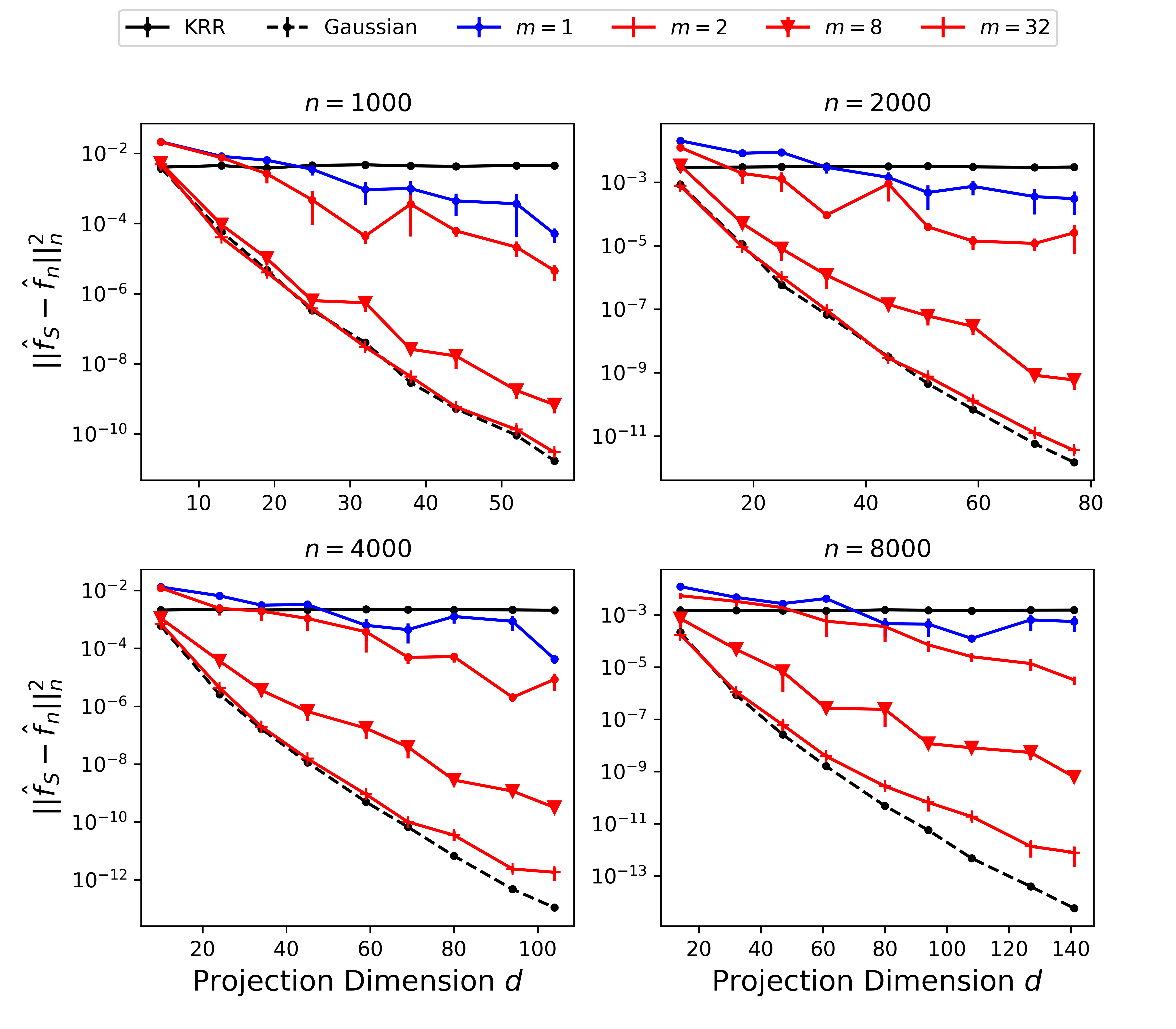
Figure 2: Approximation Errors of Different Methods

In Figure 2, we actually take the Nyström method ($m=1$, the blue solid line) and the Gaussian sketching method ($m=\infty$, the black dashed line) as two benchmarks. The estimation error $\|\hat{f}_{n}-f^{\ast}\|_{n}^{2}$ of the original KRR (the black solid line) is also provided in the figure as a reference. As expected, with the same projection dimension $d$, Gaussian sketches attain the approximation error orders of magnitude lower than the Nyström method. However, as implied by Theorem 3.6, with a medium $m\leq 32$ the approximation error can be reduced to a similar scale as the Gaussian sketch. The phenomenon validates the effectiveness of Theorem 3.6, and suggests that in practice a medium $m$ is enough to make our sketching method as accurate as Gaussian sketching.

4.2 Accuracy versus efficiency trade-off

To show the improvement on the comprehensive performance, we evaluate our method on RadiusQueriesAggregation (Savva et al., 2018; Anagnostopoulos et al., 2018)(denoted by RQA), a dataset downloaded from the UCI ML Repository (Dua and Graff, 2017). This dataset contains 200000 data points and 4 features. Due to the space limit, here we only present a partial result, and the rest parts will be provided in the appendix.

To show the evolving trend, we set a sequence of sample sizes beforehand and in each round run the experiment on a subset of the whole data points with the given sample size $n$. The testing errors are estimated on a random subset ($20\%$ of the original dataset) which is not used in the training. We begin by normalizing the features to have variance $1$ in the randomly drawn dataset, before obtaining the empirical kernel matrix using Matérn kernel (the smoothness parameter $\nu=1.5$). The regularization parameter $\lambda$ of KRR is $0.9\cdot n^{-7/11}$. We set the projection dimension as $\lfloor 1.5\cdot n^{4/11}\rfloor$ for all sketching methods. The candidate methods include the Gaussian sketching method, very sparse random projection (Li et al., 2006), the Nyström method with BLESS (Rudi et al., 2018), and our accumulation method with $m=4$. All the results reported below in Figure 3 are averaged over 30 replicates, and the error bars are computed as before.

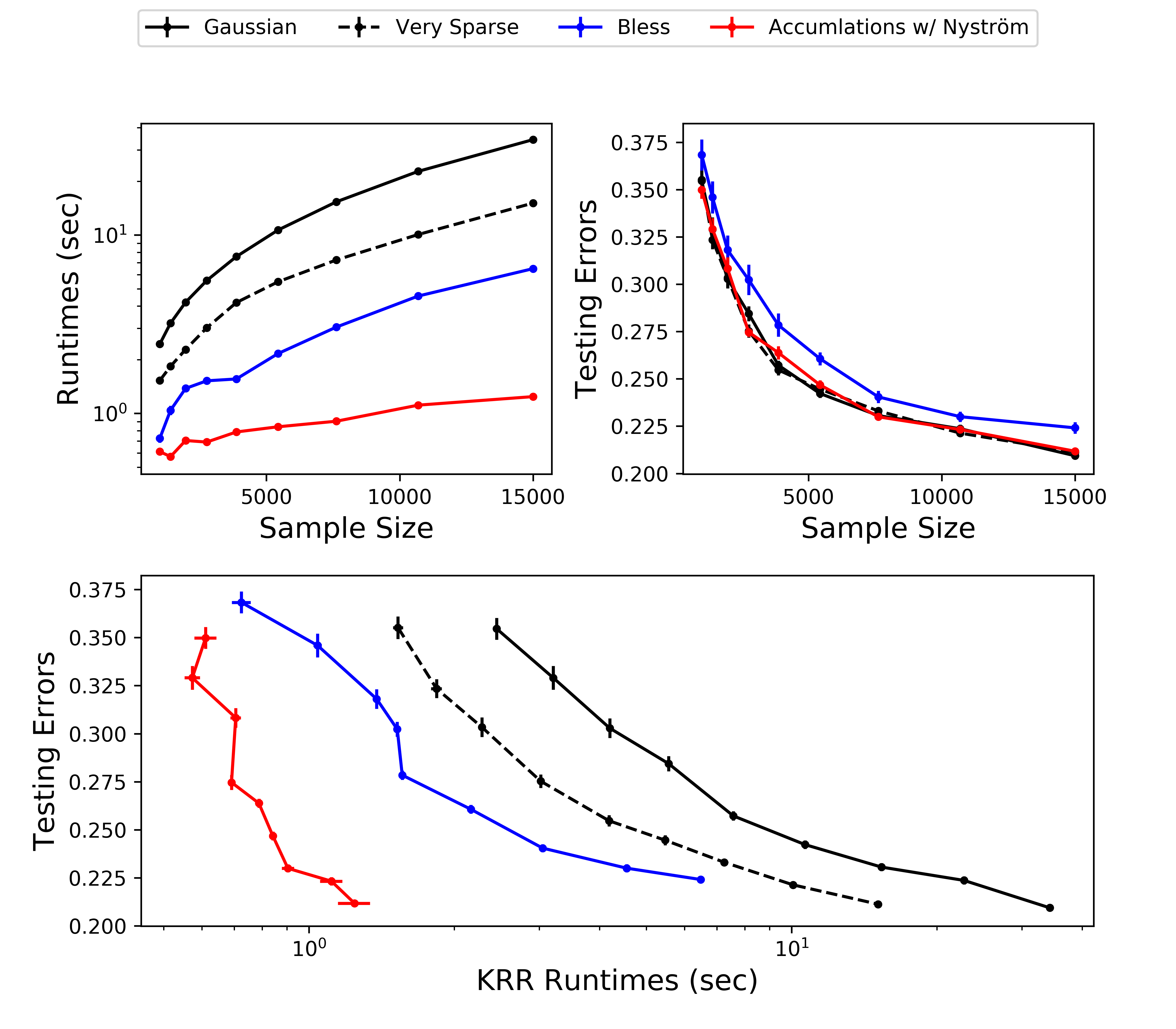
Figure 3: Trade-off between Accuracy and Efficiency

In Figure 3 we compare the comprehensive performance of those methods. The comprehensive performance is composed of two factors, statistical accuracy, and computational efficiency. As we can see in the last subplot of Figure 3, our method attains the best trade-off between in-sample error and runtime among all the candidate methods. Taking a closer look, we can even observe that our method achieves the advantages of the two extremes in our framework: it can attain an accuracy similar to Gaussian sketching, and enjoy the low runtime of the same order as the Nyström method. As for very sparse random projection, since it is designed for a general matrix and does not utilize the leverage information, its performance falls somewhere in between the above-described methods. We ascribe the remarkable performance of our method to the proper sparsity of the sketching matrix and the high efficiency of the matrix addition.

4.3 Additional empirical results

In the appendix, we verify the effect of our method on the other two datasets PPGasEmission (KAYA et al., 2019) and CASP (Dua and Graff, 2017), and also confirm the usage of Falkon (Rudi et al., 2017) does not affect the main claim above. Basically, those experiments demonstrate that in practice, a medium $m$ substantially improves the accuracy of the classical Nyström method with uniform sub-sampling distribution, and the extra cost is much lower compared to other advanced methods.

5 Conclusion and future work

We have introduced a unified framework for randomized sketches in kernel ridge regression. This framework unifies two common methods, sub-Gaussian and sub-sampling sketching, by introducing an accumulation parameter $m$. Our theoretical results state that a medium $m$ improves the prediction performance of the approximate KRR, while still maintaining a low projection dimension even when the sub-sampling probability $p_{i}$’s are not optimal. The empirical experiments complement our theory by showing that our proposed method with medium $m$ and simple uniform sampling scheme can achieve high accuracy close to sub-Gaussian sketching, and be as efficient as sub-sampling-based sketching.

One possible extension of our work is applying the proposed sketching method to approximate matrix multiplication and how the approximation error translates when the new sketching method is utilized to approximate some classical machine learning models, such as $k$-means and PCA. Another direction of future research is the extension of our method to broader classes of positive semidefinite kernels, for example graph kernels (Vishwanathan et al., 2010) and string kernels (Vishwanathan and Smola, 2002).

This work is supported by NSF grant DMS-1810831.

Appendix A APPENDIX OUTLINE

This appendix is arranged as follows. In Section B, we introduce some useful facts to help illustrate the assumptions in Theorem 3.4 in the main paper, and some matrix inequalities to prepare for the proof in Section C. With those matrix inequalities, we prove Theorem 3.6 in the main paper, the condition to guarantee $K$-satisfiability with high probability. Finally, in Section D, we provide more details on the experiments in the main paper, and some additional experiments to comprehensively compare our sketching method with the other candidates.

Appendix B USEFUL FACTS

In this section, we will first introduce some preliminary knowledge of RKHS kernels, and then provide some useful matrix inequalities heavily used later.

B.1 Preliminaries

Theorem 3.4 in the main paper guarantees that for a $K$-satisfiable sketching matrix $S$, with high probability the approximation error $\|\hat{f}_{S}-\hat{f}_{n}\|_{n}^{2}$ would be bounded by $\lambda+\frac{d_{\lambda}}{n}$. The result of this theorem is powerful, while it relies on some assumptions on the kernel function and the sketching matrix used. The authors of the previous work (Liu et al., 2018) have summarized three assumptions for Theorem 3.4, and in this subsection, we provide the necessary introduction to the eigendecomposition of the kernel function $\mathcal{K}$, to ease the explanation of the assumptions.

In the preliminaries in the main paper, we have known that the associated kernel function $\mathcal{K}$ of an RKHS $\mathbb{H}$ is positive semi-definite. Further by Mercer’s theorem, $\mathcal{K}$ has the following spectral expansion:

$$\mathcal{K}(x,x^{\prime})=\sum_{i=1}^{\infty}\mu_{i}\phi_{i}(x)\phi_{i}(x^{\prime}),\quad\forall x,x^{\prime}\in\mathcal{X},$$

where $\mu_{1}\geq\mu_{2}\geq\cdots\geq 0$ are denoted as the eigenvalues of $\mathcal{K}$, and $\{\phi_{i}\}_{i=1}^{\infty}$ actually form a basis in $L^{2}(\mathcal{X})$, i.e.

$$\left\langle\phi_{i},\phi_{j}\right\rangle_{L^{2}(\mathcal{X})}=\delta_{ij},\quad\left\langle\phi_{i},\phi_{j}\right\rangle_{\mathbb{H}}=\delta_{ij}/\mu_{i}.$$

The eigenvalues $\{\mu_{i}\}_{i=1}^{\infty}$ of the kernel function $\mathcal{K}$ are closely related to the eigenvalues $\{\sigma_{i}\}_{i=1}^{n}$ of the rescaled empirical kernel matrix $\frac{1}{n}K$. The eigenvalue pair $(\mu_{i},\sigma_{i})$ of the same index $i$ would roughly have the same magnitude, and more details can be found in the work (Braun, 2006).

B.2 Useful Matrix Inequalities

The key step in the proof of $K$-satisfiability is to control the operator norm of a random matrix. Here we give a sequence of matrix inequalities used later in Section C. More details and proofs of those matrix inequalities could be found in the note (Tropp, 2012).

Theorem B.1 (Matrix Chernoff).

Consider a finite sequence $\{{X}_{k}\}$ of independent, random, self-adjoint matrices with dimension $n$. Assume that each random matrix satisfies

$${X}_{k}\succcurlyeq\bm{0}\quad\text{and}\quad\lambda_{\max}({X}_{k})\leq R\quad\text{almost surely}.$$

Define

$$\mu_{\max}\vcentcolon=\lambda_{\max}\left(\sum\nolimits_{k}\operatorname{\mathbb{E}}{X}_{k}\right).$$

Then for $\delta>0$,

$$\mathbb{P}\left\{{\lambda_{\max}\left(\sum\nolimits_{k}{X}_{k}\right)\geq(1+\delta)\mu_{\max}}\right\}\leq n\cdot\left[\frac{\mathrm{e}^{-\delta}}{(1+\delta)^{1+\delta}}\right]^{\mu_{\max}/R}.$$

The matrix Chernoff inequalities describe the behavior of a sum of independent, random, positive-semidefinite matrices. Specifically, they are well suited to study the operator norm of an arbitrary random matrix ${A}$ with independent columns $a_{k}$’s, due to the fact $\|{A}\|^{2}=\|{A}{A}^{T}\|=\|\sum\nolimits_{k}a_{k}a_{k}^{T}\|$, and the property that $(a_{k}a_{k}^{T})$’s are independent, random, self-adjoint matrices.

We also introduce Bernstein matrix inequality to show the normal concentration near the mean of the random matrices.

Theorem B.2 (Matrix Bernstein).

Consider a finite sequence $\{{X}_{k}\}$ of independent, random, self-adjoint matrices with dimension $n$. Assume that each random matrix satisfies

$$\operatorname{\mathbb{E}}{X}_{k}=\bm{0}\quad\text{and}\quad\|{X}_{k}\|\leq R\quad\text{almost surely}.$$

Then, for all $t\geq 0$,

$$\mathbb{P}\left\{{\|\sum\nolimits_{k}{X}_{k}\|\geq t}\right\}\leq 2n\cdot\exp\left(\frac{-t^{2}/2}{\sigma^{2}+Rt/3}\right)\quad\text{where}\quad\sigma^{2}\geq\left\|\sum\nolimits_{k}\operatorname{\mathbb{E}}\big{(}{X}_{k}^{2}\big{)}\right\|.$$

Similar to the ordinary Bernstein inequality for random variables, the decaying rate of the tail of the sum would be determined by the variance of the matrix sum and the uniform bound on the maximum eigenvalue of each summand. As in our framework, each column of $S$ is also an accumulation of $m$ independent columns, we further introduce a rectangular version of the matrix Bernstein inequality, which is an immediate corollary of Theorem B.2.

Theorem B.3 (Matrix Bernstein: Rectangular Case).

Consider a finite sequence $\{{Z}_{k}\}$ of independent, random matrices with dimensions $n_{1}\times n_{2}$. Assume that each random matrix satisfies

$$\operatorname{\mathbb{E}}{Z}_{k}=\bm{0}\quad\text{and}\quad\left\|{Z}_{k}\right\|\leq R\quad\text{almost surely}.$$

Define

$$\sigma^{2}:=\max\left\{\left\|\sum\nolimits_{k}\operatorname{\mathbb{E}}({Z}_{k}{Z}_{k}^{*})\right\|,\ \left\|\sum\nolimits_{k}\operatorname{\mathbb{E}}({Z}_{k}^{*}{Z}_{k})\right\|\right\}.$$

Then, for all $t\geq 0$,

$$\mathbb{P}\left\{{\left\|\sum\nolimits_{k}{Z}_{k}\right\|\geq t}\right\}\leq(n_{1}+n_{2})\cdot\exp\left(\frac{-t^{2}/2}{\sigma^{2}+Rt/3}\right).$$

Appendix C MISSING PROOFS

In this section, we will present the proof for Theorem 3.6 in the main paper.

Proof C.1.

The main idea of the proof is to utilize Theorem B.3, the rectangular version matrix Bernstein inequality, to control the upper bound of the column $\ell_{2}$ norm in the sketching matrix $S$, and then further address the properties of the whole matrix $S$.

We start with the first condition in $K$-satisfiability. Observing the form of the matrix $U_{1}^{T}SS^{T}U_{1}-I$, we find its expectation is zero and thus matrix Bernstein inequality (Theorem B.2) can be applied. Before that, we need to give a high probability operator norm upper bound $R$ for the summand $U_{1}^{T}S_{k}S_{k}^{T}U_{1}-I/d$, which can be derived from the norm upper bound for the vector $U_{1}^{T}S_{k}$.

Based on Algorithm 1 in the main paper, $S_{k}$ can be decomposed as

$$S_{k}=\sum_{j=1}^{m}\frac{1}{\sqrt{m}}S_{k,j},\quad\forall k\in[d],$$

where $S_{k,j}$ is a single sub-sampling column which would be $\frac{1}{\sqrt{dp_{i}}}e_{i}$ with probability $p_{i}$. We take $\frac{1}{\sqrt{m}}U_{1}^{T}S_{k,j}$’s as the random matrices and apply Theorem B.3 to them. We then need to specify the parameters $R$ and $\sigma^{2}$ in Theorem B.3. Here we let $R=\sqrt{\frac{2M}{md}}$, as $M\geq\max_{i}\frac{\|\tilde{\psi}_{i}\|^{2}}{p_{i}}\geq\max_{i}\frac{\|\tilde{u}_{i}\|^{2}}{2p_{i}}$, where $\tilde{u}_{i}$ is the sub-vector of the first $d_{\delta}$ elements in the $i$-th column $u_{i}$ of $U$. We can verify $R\geq\|\frac{1}{\sqrt{m}}U_{1}^{T}S_{k,j}\|,\forall j\in[m]$. Another parameter $\sigma^{2}=\frac{d_{\delta}}{d}$ is induced by the fact $\operatorname{\mathbb{E}}S_{k,j}S_{k,j}^{T}=\frac{1}{d}I$.

By Theorem B.3 we have the following probability inequality

$$\mathbb{P}\left\{{\|U_{1}^{T}S_{k}\|>t}\right\}\leq(d_{\delta}+1)\exp(\frac{-t^{2}/2}{\frac{d_{\delta}}{d}+\sqrt{\frac{2M}{md}}t/3}),$$

and further by union bound we obtain

$$\mathbb{P}\left\{{\max_{k\in[d]}\|U_{1}^{T}S_{k}\|>t}\right\} \leq d(d_{\delta}+1)\exp(\frac{-t^{2}/2}{\frac{d_{\delta}}{d}+\sqrt{\frac{2M}{md}}t/3})$$

$$\mathbb{P}\left\{{\max_{k\in[d]}\|U_{1}^{T}S_{k}\|>t=\frac{1}{3}uR+\sqrt{\frac{1}{9}u^{2}R^{2}+2u\sigma^{2}}}\right\} \leq d(d_{\delta}+1)\exp(-u),$$

where we substitute $u$ for $t$ in the last inequality to better control the probability. After the substitution, we upper bound the right hand side by $\rho/4$, and have $u\sim\log\frac{n}{\rho}$. Thus with probability $1-\frac{\rho}{4}$, we upper bound the vector norm $\|U_{1}^{T}S_{k}\|$ by $t$, and further bound the norm of the zero mean matrix $\|U_{1}^{T}S_{k}S_{k}^{T}U_{1}-\frac{1}{d}I\|$ by $t^{2}$.

For the simplicity of notation, we would denote $U_{1}^{T}S_{k}S_{k}^{T}U_{1}-\frac{1}{d}I$ as $X_{k}$ in this paragraph. We still need to control $\|\operatorname{\mathbb{E}}X_{k}^{2}\|$ to apply Theorem B.2. We first expand $\operatorname{\mathbb{E}}X_{k}^{2}$ as

$$\operatorname{\mathbb{E}}X_{k}^{2}=\operatorname{\mathbb{E}}\sum_{i_{1},i_{2},i_{3},i_{4}\in[n]}(\frac{Z_{i_{1}}Z_{i_{2}}}{md}-\frac{\delta_{i_{1}i_{2}}}{d})(\frac{Z_{i_{3}}Z_{i_{4}}}{md}-\frac{\delta_{i_{3}i_{4}}}{d})\tilde{u}_{i_{1}}\tilde{u}_{i_{2}}^{T}\tilde{u}_{i_{3}}\tilde{u}_{i_{4}}^{T},$$ (5)

where $S_{k}^{T}=\frac{1}{\sqrt{md}}(Z_{1},Z_{2},\cdots,Z_{n})$, and further $Z_{i}=\frac{1}{\sqrt{p_{i}}}\sum_{j=1}^{m}Z_{ij}$, where $Z_{ij}$’s are i.i.d and they would be $\pm 1$ with probability $\frac{p_{i}}{2}$ respectively, or be $0$ with probability $1-p_{i}$. The setting represents the fact that $S_{k}$ is the accumulation of $m$ independent columns $\frac{1}{\sqrt{m}}S_{k,j}$. By some calculation, we have $\operatorname{\mathbb{E}}Z_{i_{1}}Z_{i_{2}}=m\delta_{i_{1}i_{2}}$, and for most combination of $i_{1},i_{2},i_{3},i_{4}$ the summand in equation (5) would be zero. To exactly compute equation (5), we only need to consider the following four cases:

1. $i_{1}=i_{2}=i_{3}=i_{4}$,

2. $i_{1}=i_{2}\neq i_{3}=i_{4}$,

3. $i_{1}=i_{3}\neq i_{2}=i_{4}$,

4. $i_{1}=i_{4}\neq i_{2}=i_{3}$.

For the first case, we have

$$\operatorname{\mathbb{E}}\sum_{i_{1}=i_{2}=i_{3}=i_{4}}(\frac{Z_{i_{1}}^{2}}{md}-\frac{1}{d})^{2}\tilde{u}_{i_{1}}\tilde{u}_{i_{1}}^{T}\tilde{u}_{i_{1}}\tilde{u}_{i_{1}}^{T}=\frac{1}{d^{2}}\sum_{i=1}^{n}(\frac{1}{mp_{i}}+\frac{3(m-1)}{m}-1)\tilde{u}_{i_{1}}\tilde{u}_{i_{1}}^{T}\tilde{u}_{i_{1}}\tilde{u}_{i_{1}}^{T};$$

for the second case we have

$$\operatorname{\mathbb{E}}\sum_{i_{1}=i_{2}\neq i_{3}=i_{4}}(\frac{Z_{i_{1}}^{2}}{md}-\frac{1}{d})(\frac{Z_{i_{3}}^{2}}{md}-\frac{1}{d})\tilde{u}_{i_{1}}\tilde{u}_{i_{1}}^{T}\tilde{u}_{i_{3}}\tilde{u}_{i_{3}}^{T}=-\frac{1}{md^{2}}\sum_{i_{1}\neq i_{3}}\tilde{u}_{i_{1}}\tilde{u}_{i_{1}}^{T}\tilde{u}_{i_{3}}\tilde{u}_{i_{3}}^{T};$$

for the third case we have

$$\operatorname{\mathbb{E}}\sum_{i_{1}=i_{3}\neq i_{2}=i_{4}}(\frac{Z_{i_{1}}Z_{i_{2}}}{md})^{2}\tilde{u}_{i_{1}}\tilde{u}_{i_{2}}^{T}\tilde{u}_{i_{1}}\tilde{u}_{i_{2}}^{T}=\frac{m-1}{md^{2}}\sum_{i_{1}\neq i_{2}}\tilde{u}_{i_{1}}\tilde{u}_{i_{2}}^{T}\tilde{u}_{i_{1}}\tilde{u}_{i_{2}}^{T};$$

for the fourth case we have

$$\operatorname{\mathbb{E}}\sum_{i_{1}=i_{4}\neq i_{2}=i_{3}}(\frac{Z_{i_{1}}Z_{i_{2}}}{md})^{2}\tilde{u}_{i_{1}}\tilde{u}_{i_{2}}^{T}\tilde{u}_{i_{2}}\tilde{u}_{i_{1}}^{T}=\frac{m-1}{md^{2}}\sum_{i_{1}\neq i_{2}}\tilde{u}_{i_{1}}\tilde{u}_{i_{2}}^{T}\tilde{u}_{i_{2}}\tilde{u}_{i_{1}}^{T}.$$

Combining the pieces together, we obtain

$$\operatorname{\mathbb{E}}X_{k}^{2}=\frac{1}{md^{2}}\sum_{i=1}^{n}\frac{\|\tilde{u}_{i}\|^{2}}{p_{i}}\tilde{u}_{i_{1}}\tilde{u}_{i_{1}}^{T}+\frac{m-1}{md^{2}}d_{\delta}I+\frac{m-2}{md^{2}}I,$$

which implies

$$\|\operatorname{\mathbb{E}}X_{k}^{2}\|\leq\frac{1}{d^{2}}(\frac{2}{m}M+\frac{m-1}{m}d_{\delta}+\frac{m-2}{m}),$$

and hence we let $\|\sum_{k}\operatorname{\mathbb{E}}X_{k}^{2}\|\leq\sigma_{b}^{2}\vcentcolon=\frac{1}{d}(\frac{2}{m}M+d_{\delta}+1)$.

Applying Theorem B.2, we have the following probability inequality:

$$\mathbb{P}\left\{{\|U_{1}^{T}SS^{T}U_{1}-I_{d_{\delta}}\|_{op}\geq 1/2}\right\}\leq 2d_{\delta}\exp(\frac{-1/8}{\sigma_{b}^{2}+\frac{1}{6}t^{2}})\leq\frac{\rho}{4}.$$

To make the last inequality hold, we need

$$\sigma_{b}^{2}+\frac{1}{6}t^{2}\lesssim 1/\log\frac{n}{\rho},$$

which turns out to imply

$$d \gtrsim d_{\delta}\log^{2}(\frac{n}{\rho})$$

$$md \gtrsim M\log^{3}(\frac{n}{\rho}).$$

To complete the proof for the theorem, we still need to validate the requirements on $m,d$ above can induce the second condition in $K$-satisfiability. We first rewrite the target $\|S^{T}U_{2}\Sigma_{2}^{\frac{1}{2}}\|$ as $\|\overline{(\Sigma+\delta I)}^{\frac{1}{2}}\Psi_{\delta}S\|$, where $\overline{(\Sigma+\delta I)}^{\frac{1}{2}}$ means the matrix $\Sigma+\delta I$ would set the first $d_{\delta}$ diagonal elements as zero and only keep the rest ones.

As above we start with the control over the maximal norm of the column $\overline{(\Sigma+\delta I)}^{\frac{1}{2}}\Psi_{\delta}S_{k}$. For simplicity we will reuse the notation $\sigma^{2},R$ to apply Theorem B.3. Recall $S_{k}=\sum_{j=1}^{m}\frac{1}{\sqrt{m}}S_{k,j}$, this time $\|\frac{1}{\sqrt{m}}\overline{(\Sigma+\delta I)}^{\frac{1}{2}}\Psi_{\delta}S_{k,j}\|$ is bounded by

$$\frac{1}{\sqrt{md}}\sqrt{2\delta}\sqrt{\max_{i}\frac{\|\psi_{i}\|^{2}-\|\tilde{\psi}_{i}\|^{2}}{p_{i}}}\leq R\vcentcolon=\sqrt{\frac{2\delta M}{md}},$$

and

$$\operatorname{\mathbb{E}}\sum_{j}\frac{1}{{m}}S_{k,j}^{T}\Psi_{\delta}^{T}\overline{(\Sigma+\delta I)}\Psi_{\delta}S_{k,j}=\frac{{\rm Tr}(\Sigma_{2})}{d}\leq\sigma^{2}\vcentcolon=\frac{Cd_{\delta}}{d}\delta,$$

in which the last inequality is induced by the fast eigenvalue decay rate in Assumption 3.2 (Liu et al., 2018, Lemma 3.1). Again by Theorem B.3 and the union bound, we have

$$\mathbb{P}\left\{{\max_{k\in[d]}\|\Sigma_{2}U_{2}^{T}S_{k}\|>t=\frac{1}{3}uR+\sqrt{\frac{1}{9}u^{2}R^{2}+2u\sigma^{2}}}\right\} \leq d(n+1)\exp(-u)\leq\rho/4.$$

Given the high probability norm upper bound $t$, to apply Theorem B.1 we re-define ${X}_{k}=\overline{\Sigma}^{\frac{1}{2}}U^{T}S_{k}S_{k}^{T}U\overline{\Sigma}^{\frac{1}{2}}$, and $\mu_{\max}=\lambda_{\max}\left(\sum\nolimits_{k}\operatorname{\mathbb{E}}{X}_{k}\right)=\delta$. We finally have

$$\mathbb{P}\left\{{\lambda_{\max}\left(\sum\nolimits_{k}{X}_{k}\right)\geq(1+1)\mu_{\max}}\right\}\leq n\cdot\left[\frac{\mathrm{e}^{-1}}{4}\right]^{\mu_{\max}/t^{2}}\leq\rho/4.$$

To make the second condition in $K$-satisfiability hold we only need to validate

$$t^{2}/\delta\lesssim 1/\log\frac{n}{\rho},$$

which is actually satisfied by the derived requirements on $m,d$ above.

Appendix D MORE ON SIMULATIONS

In this section, we provide the complete experiment settings and several additional figures to further illustrate our method.

D.1 Experiment Settings in Figure 1 in the Main Paper

This figure is only shown for illustration, and the settings are relatively simple. In Figure 1 we consider three representative sketching methods, the Gaussian sketching method, the classical Nyström method, and our accumulation method with $m=5$. We compare the estimation error $\|\hat{f}_{S}-\hat{f}_{n}\|_{n}^{2}$ of each other and also report the total runtime in Figure 1.

Specifically, we run the experiment on a bimodal distribution over $\mathbb{R}^{3}$. The bimodal distribution has two components: with probability $\frac{n}{n+n^{\gamma}}$ generating a Unif$[0,1]^{3}$; and with probability $\frac{n^{\gamma}}{n+n^{\gamma}}$ generating a random variable with pdf $\prod_{j=1}^{3}(5-2x_{j})$ for $x_{j}\in[2,2.5]$, where $n$ is the sample size varying from $n=1,000$ to $16,000$ and $\gamma=0.5$. In addition, by cross validation the Matérn kernel with smoothness parameter $\nu=0.5$ is chosen, and the regularization parameter of the KRR $\lambda$ is set as $0.3n^{-\frac{4}{7}}$. The true regression function we use is $f^{\ast}(x)=g(\|x\|/3)$, with

$$g(x)=1.6|(x-0.4)(x-0.6)|-x(x-1)(x-2)-0.5,$$

and i.i.d. noises follow $\mathcal{N}(0,0.25)$. We use uniform sub-sampling distribution for all the applicable methods, and the projection dimension $d$ is chosen as $\lfloor 1.3n^{\frac{3}{7}}\rfloor$. The results finally reported in Figure 1 are averaged over 30 replicates.

D.2 Experiment Settings in Figure 2 in the Main Paper

In this experiment, we compare the approximation error $\|\hat{f}_{S}-\hat{f}_{n}\|_{n}^{2}$ among the KRR estimators obtained by the sketching matrices with different $m$, including the Gaussian sketch as an instance of $m=\infty$. As above, we run the experiment on a bimodal distribution over $\mathbb{R}^{3}$. The bimodal distribution has two components: with probability $\frac{n}{n+n^{\gamma}}$ generating a Unif$[0,1]^{3}$; and with probability $\frac{n^{\gamma}}{n+n^{\gamma}}$ generating a random variable with pdf $\prod_{j=1}^{3}(5-2x_{j})$ for $x_{j}\in[2,2.5]$, where $n$ is the sample size varying from $n=1,000$ to $8,000$ and $\gamma=0.6$. In addition, by cross validation the Gaussian kernel with bandwidth $\sigma=1.5n^{-\frac{1}{7}}$ is chosen, and the regularization parameter of the KRR $\lambda$ is set as $0.5n^{-\frac{4}{7}}$. The true regression function $f^{\ast}$ we use is $f^{\ast}(x)=g(\|x\|/3)$, with

$$g(x)=1.6|(x-0.4)(x-0.6)|-x(x-1)(x-2)-0.5,$$

and i.i.d. noises follow $\mathcal{N}(0,0.25)$. We use uniform sub-sampling distribution for all the applicable methods, and the projection dimension $d$ varies from $\lfloor 0.3n^{\frac{3}{7}}\rfloor$ to $\lfloor 3n^{\frac{3}{7}}\rfloor$. The results reported in Figure 2 are averaged over 30 replicates.

D.3 Additional Experiments and Experiment Settings in Figure 3 in the Main Paper

As mentioned in the main paper, we evaluate the comprehensive performance of our accumulation method on three real datasets and also consider the usage of Falkon (Rudi et al., 2017). Due to the space limit in the main paper, we move the complete experiment settings and results to this section and will demonstrate them as follows, including the settings in Figure 3 in the main paper.

We verify the effect of our method on three datasets, RadiusQueriesAggregation (Savva et al., 2018; Anagnostopoulos et al., 2018)(denoted by RQA), CASP (Dua and Graff, 2017), and PPGasEmission (KAYA et al., 2019)(denoted by GAS), all downloaded from the UCI ML Repository (Dua and Graff, 2017). For those datasets, RQA contains $200,000$ data points and $4$ features; CASP contains $45,730$ data points and $9$ features; GAS contains $36,733$ data points and $10$ features; in this subsection we use $d_{X}$ to represent the number of the features. To show the evolving trend, we set a sequence of sample sizes beforehand (from $1,000$ to $15,000$, at the limit of our computational feasibility) and in each round run the experiment on a subset of the whole data points with the given sample size $n$. The testing errors are estimated on a random subset ($20\%$ of the original dataset) which is not used in the training. We begin by normalizing the features to have variance $1$ in the randomly drawn dataset, before obtaining the empirical kernel matrix using Matérn kernel (the smoothness parameter $\nu=1.5$). The regularization parameter $\lambda$ of KRR is $0.9\cdot n^{-\frac{3+d_{X}}{3+2d_{X}}}$. We set the projection dimension as $\lfloor 1.5\cdot n^{\frac{d_{X}}{3+2d_{X}}}\rfloor$ for all sketching methods. The candidate methods include the Gaussian sketching method, very sparse random projection (Li et al., 2006), the Nyström method with Bless (Rudi et al., 2018), and our accumulation method with $m=4$. Among all the experiments, the number of sub-samples used in Bless is chosen as $\lfloor 3\cdot n^{\frac{d_{X}}{3+2d_{X}}}\rfloor$. The usage of Falkon (Rudi et al., 2017) is also considered, and we provide some experimental results to show our method still attain the optimal trade-off between statistical accuracy and computational efficiency. All the results reported below in Figure 4 (in which the first subplot is Figure 3 in the main paper) and Figure 5 are averaged over 30 replicates.

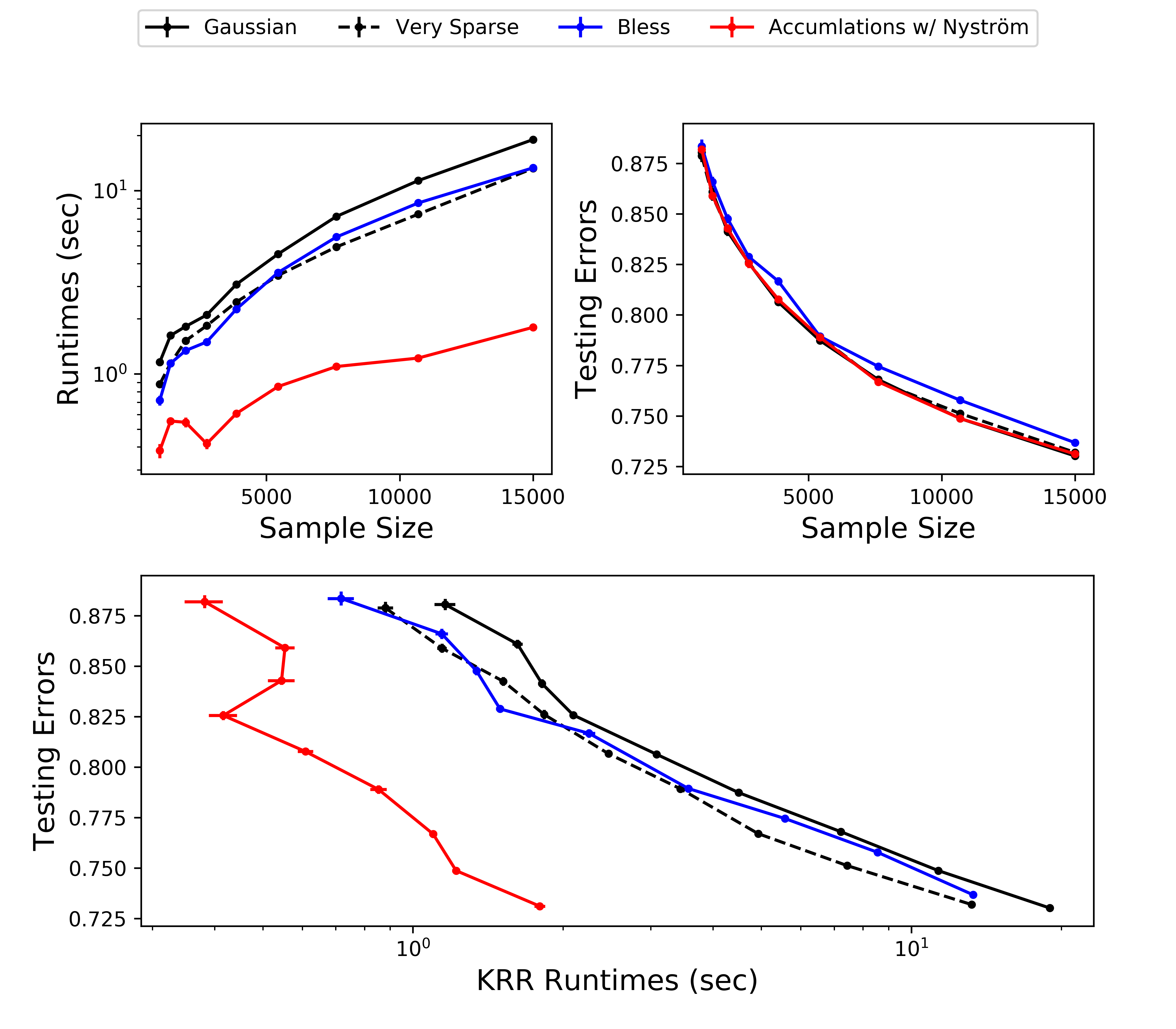
[RQA]  [CASP]  [GAS]

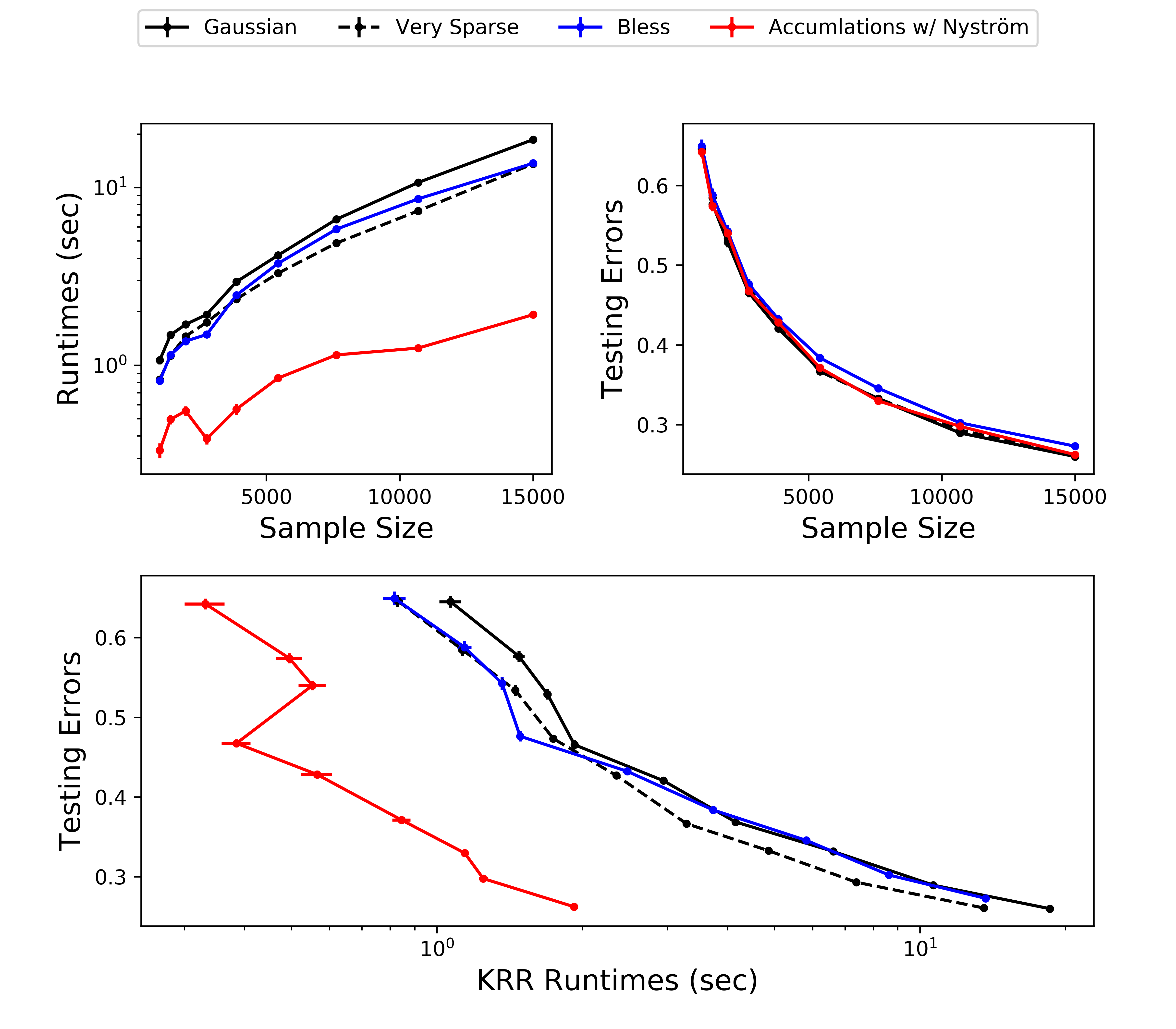
Figure 4: Trade-off between Accuracy and Efficiency without Falkon

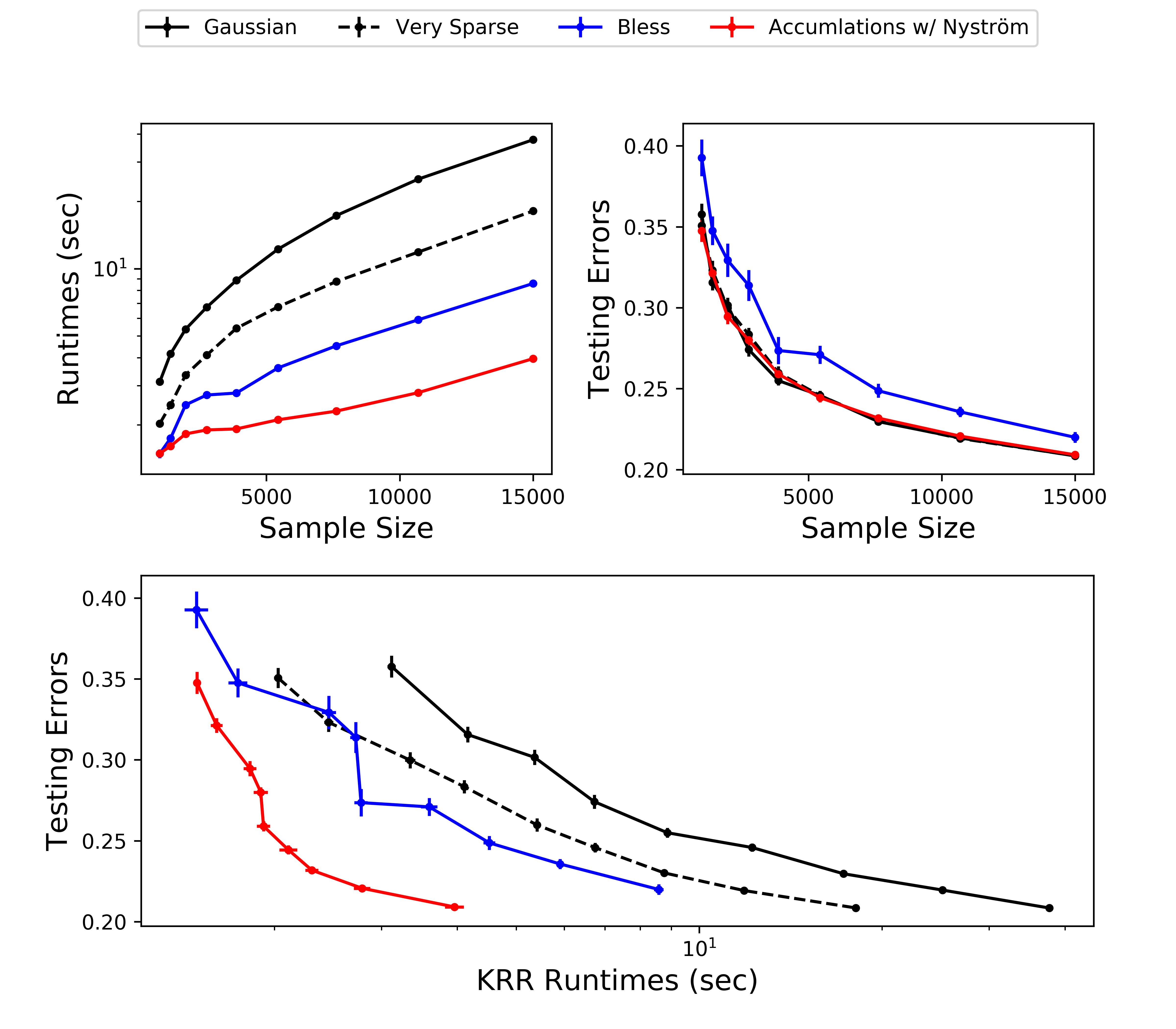
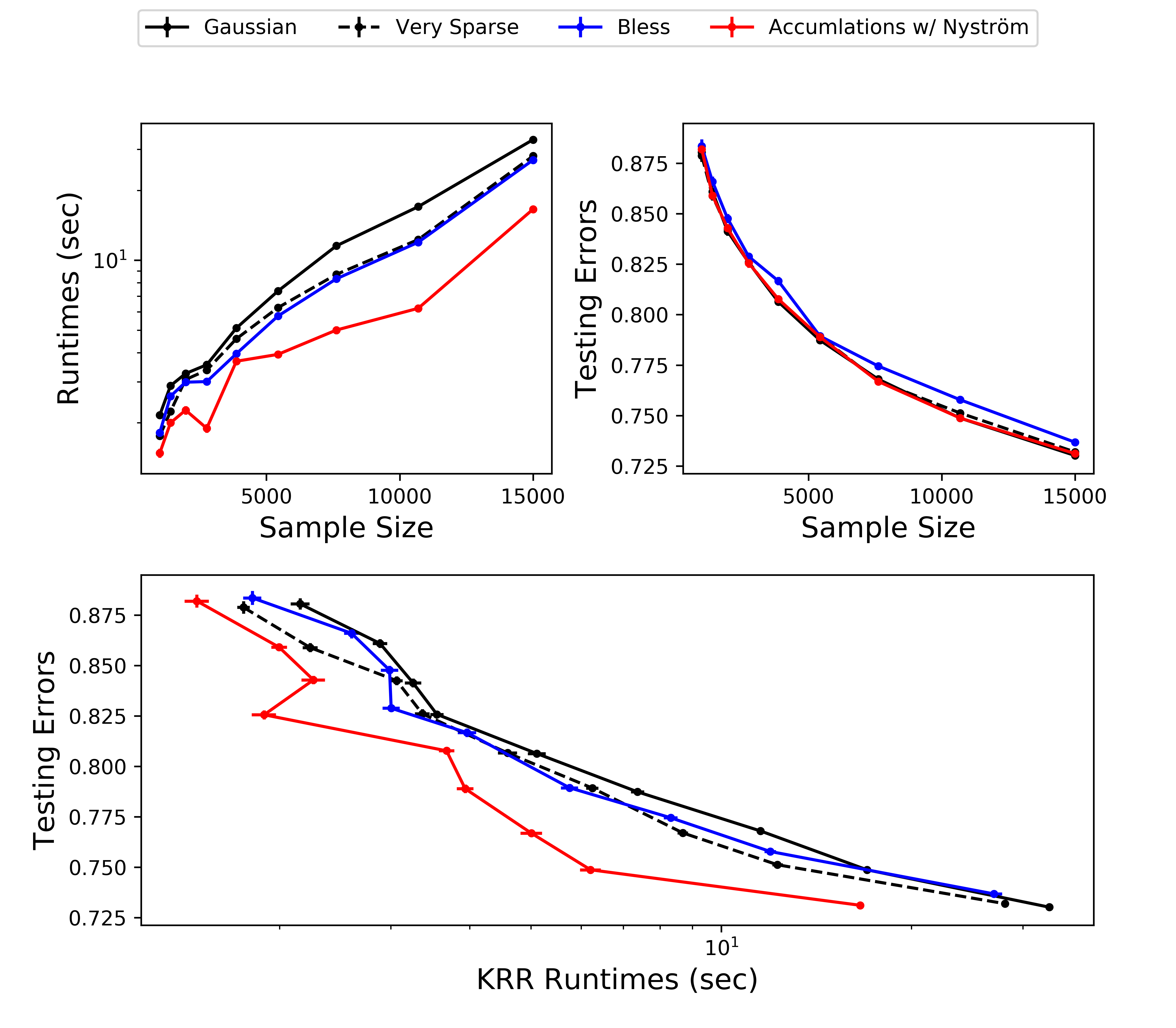
[RQA]  [CASP]  [GAS]

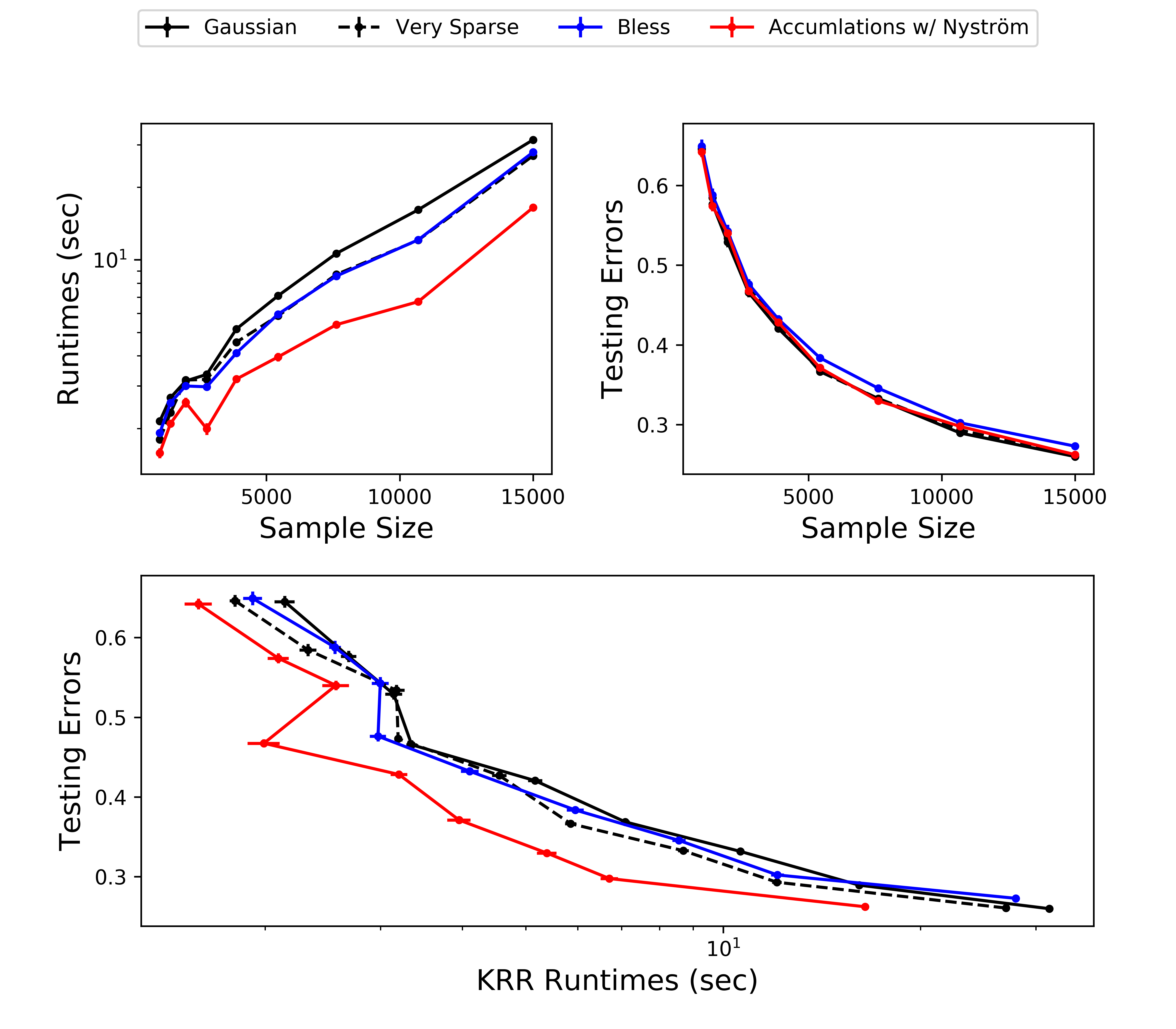
Figure 5: Trade-off between Accuracy and Efficiency with Falkon

Basically, those experiments demonstrate that in practice, a medium $m$ could substantially improve the accuracy of the classical Nyström method with uniform sub-sampling distribution, and the extra cost is much lower compared to other advanced methods. Specifically, all the methods above can be combined with a fast KRR solving method Falkon. Under our experiment settings, Falkon maintains the estimation accuracy, while not accelerate the training much since the sample size is not large enough. As shown in Figure 5, the usage of Falkon would not change the main conclusion that our accumulation method (the red solid curve) provides the optimal trade-off between statistical accuracy and computational efficiency, among all the candidate sketching methods.

References

- Achlioptas (2003) Dimitris Achlioptas. Database-friendly random projections: Johnson-lindenstrauss with binary coins. Journal of computer and System Sciences, 66(4):671–687, 2003.
- Ahle et al. (2020) Thomas D Ahle, Michael Kapralov, Jakob BT Knudsen, Rasmus Pagh, Ameya Velingker, David P Woodruff, and Amir Zandieh. Oblivious sketching of high-degree polynomial kernels. In Proceedings of the Fourteenth Annual ACM-SIAM Symposium on Discrete Algorithms, pages 141–160. SIAM, 2020.
- Alaoui and Mahoney (2015) Ahmed Alaoui and Michael W Mahoney. Fast randomized kernel ridge regression with statistical guarantees. In Advances in Neural Information Processing Systems, pages 775–783, 2015.
- Anagnostopoulos et al. (2018) Christos Anagnostopoulos, Fotis Savva, and Peter Triantafillou. Scalable aggregation predictive analytics. Applied Intelligence, 48(9):2546–2567, 2018.
- Arriaga and Vempala (1999) Rosa I Arriaga and Santosh Vempala. An algorithmic theory of learning: Robust concepts and random projection. In 40th Annual Symposium on Foundations of Computer Science (Cat. No. 99CB37039), pages 616–623. IEEE, 1999.
- Bach (2017) Francis Bach. On the equivalence between kernel quadrature rules and random feature expansions. The Journal of Machine Learning Research, 18(1):714–751, 2017.
- Braun (2006) Mikio L Braun. Accurate error bounds for the eigenvalues of the kernel matrix. Journal of Machine Learning Research, 7(Nov):2303–2328, 2006.
- Dua and Graff (2017) Dheeru Dua and Casey Graff. UCI machine learning repository, 2017. URL http://archive.ics.uci.edu/ml.
- Gittens and Mahoney (2013) Alex Gittens and Michael Mahoney. Revisiting the nystrom method for improved large-scale machine learning. In International Conference on Machine Learning, pages 567–575. PMLR, 2013.
- Hastie et al. (2005) Trevor Hastie, Robert Tibshirani, Jerome Friedman, and James Franklin. The elements of statistical learning: data mining, inference and prediction. The Mathematical Intelligencer, 27(2):83–85, 2005.
- Kanagawa et al. (2018) Motonobu Kanagawa, Philipp Hennig, Dino Sejdinovic, and Bharath K Sriperumbudur. Gaussian processes and kernel methods: A review on connections and equivalences. arXiv preprint arXiv:1807.02582, 2018.
- KAYA et al. (2019) Heysem KAYA, Pınar TÜFEKCİ, and Erdinç UZUN. Predicting CO and NOxemissions from gas turbines: novel data and abenchmark PEMS. TURKISH JOURNAL OF ELECTRICAL ENGINEERING & COMPUTER SCIENCES, 27(6):4783–4796, nov 2019. 10.3906/elk-1807-87. URL https://doi.org/10.3906%2Felk-1807-87.
- Kimeldorf and Wahba (1971) George Kimeldorf and Grace Wahba. Some results on tchebycheffian spline functions. Journal of mathematical analysis and applications, 33(1):82–95, 1971.
- Li et al. (2016) Chengtao Li, Stefanie Jegelka, and Suvrit Sra. Fast dpp sampling for nystr” om with application to kernel methods. arXiv preprint arXiv:1603.06052, 2016.
- Li et al. (2006) Ping Li, Trevor J Hastie, and Kenneth W Church. Very sparse random projections. In Proceedings of the 12th ACM SIGKDD international conference on Knowledge discovery and data mining, pages 287–296, 2006.
- Liu et al. (2018) Meimei Liu, Zuofeng Shang, and Guang Cheng. Nonparametric testing under random projection. arXiv preprint arXiv:1802.06308, 2018.
- Musco and Musco (2017) Cameron Musco and Christopher Musco. Recursive sampling for the nystrom method. In Advances in Neural Information Processing Systems, pages 3833–3845, 2017.
- Pilanci and Wainwright (2015) Mert Pilanci and Martin J Wainwright. Randomized sketches of convex programs with sharp guarantees. IEEE Transactions on Information Theory, 61(9):5096–5115, 2015.
- Rahimi and Recht (2008) Ali Rahimi and Benjamin Recht. Random features for large-scale kernel machines. In Advances in neural information processing systems, pages 1177–1184, 2008.
- Rudi et al. (2015) Alessandro Rudi, Raffaello Camoriano, and Lorenzo Rosasco. Less is more: Nyström computational regularization. In Advances in Neural Information Processing Systems, pages 1657–1665, 2015.
- Rudi et al. (2017) Alessandro Rudi, Luigi Carratino, and Lorenzo Rosasco. Falkon: An optimal large scale kernel method. In Advances in Neural Information Processing Systems, pages 3888–3898, 2017.
- Rudi et al. (2018) Alessandro Rudi, Daniele Calandriello, Luigi Carratino, and Lorenzo Rosasco. On fast leverage score sampling and optimal learning. In Advances in Neural Information Processing Systems, pages 5672–5682, 2018.
- Savva et al. (2018) Fotis Savva, Christos Anagnostopoulos, and Peter Triantafillou. Explaining aggregates for exploratory analytics. In 2018 IEEE International Conference on Big Data (Big Data), pages 478–487. IEEE, 2018.
- Shawe-Taylor et al. (2004) John Shawe-Taylor, Nello Cristianini, et al. Kernel methods for pattern analysis. Cambridge university press, 2004.
- Srinivasa et al. (2020) Rakshith S Srinivasa, Mark A Davenport, and Justin Romberg. Localized sketching for matrix multiplication and ridge regression. arXiv preprint arXiv:2003.09097, 2020.
- Stone (1982) Charles J Stone. Optimal global rates of convergence for nonparametric regression. The annals of statistics, pages 1040–1053, 1982.
- Tropp (2012) Joel A Tropp. User-friendly tail bounds for sums of random matrices. Foundations of computational mathematics, 12(4):389–434, 2012.
- Tuo et al. (2020) Rui Tuo, Yan Wang, and CF Wu. On the improved rates of convergence for mat’ern-type kernel ridge regression, with application to calibration of computer models. arXiv preprint arXiv:2001.00152, 2020.
- Vershynin (2010) Roman Vershynin. Introduction to the non-asymptotic analysis of random matrices. arXiv preprint arXiv:1011.3027, 2010.
- Vishwanathan et al. (2010) S Vichy N Vishwanathan, Nicol N Schraudolph, Risi Kondor, and Karsten M Borgwardt. Graph kernels. Journal of Machine Learning Research, 11:1201–1242, 2010.
- Vishwanathan and Smola (2002) SVN Vishwanathan and Alexander J Smola. Fast kernels for string and tree matching. In Proceedings of the 15th International Conference on Neural Information Processing Systems, pages 585–592, 2002.
- Wang and Zhang (2013) Shusen Wang and Zhihua Zhang. Improving cur matrix decomposition and the nyström approximation via adaptive sampling. The Journal of Machine Learning Research, 14(1):2729–2769, 2013.
- Williams and Seeger (2001) Christopher KI Williams and Matthias Seeger. Using the nyström method to speed up kernel machines. In Advances in neural information processing systems, pages 682–688, 2001.
- Woodruff (2014) David P Woodruff. Sketching as a tool for numerical linear algebra. arXiv preprint arXiv:1411.4357, 2014.
- Yang et al. (2017) Yun Yang, Mert Pilanci, Martin J Wainwright, et al. Randomized sketches for kernels: Fast and optimal nonparametric regression. The Annals of Statistics, 45(3):991–1023, 2017.