Simultaneously Localize, Segment and Rank the Camouflaged Objects

Abstract

Camouflage is a key defence mechanism across species that is critical to survival. Common strategies for camouflage include background matching, imitating the color and pattern of the environment, and disruptive coloration, disguising body outlines [35]. Camouflaged object detection (COD) aims to segment camouflaged objects hiding in their surroundings. Existing COD models are built upon binary ground truth to segment the camouflaged objects without illustrating the level of camouflage. In this paper, we revisit this task and argue that explicitly modeling the conspicuousness of camouflaged objects against their particular backgrounds can not only lead to a better understanding about camouflage and evolution of animals, but also provide guidance to design more sophisticated camouflage techniques. Furthermore, we observe that it is some specific parts of the camouflaged objects that make them detectable by predators. With the above understanding about camouflaged objects, we present the first ranking based COD network (Rank-Net) to simultaneously localize, segment and rank camouflaged objects. The localization model is proposed to find the discriminative regions that make the camouflaged object obvious. The segmentation model segments the full scope of the camouflaged objects. Further, the ranking model infers the detectability of different camouflaged objects. Moreover, we contribute a large COD testing set to evaluate the generalization ability of COD models. Experimental results show that our model achieves new state-of-the-art, leading to a more interpretable COD network.

1 Introduction

Camouflage is one of the most important anti-predator defences that prevents the prey from being recognized by predators [41]. Two main strategies have been widely used among prey to become camouflaged, namely background matching and disruptive coloration [35]. The prey that rely on the former approach usually share similar color or pattern with their habitats, while for complex habitats, the background matching approach may increase their visibility. Disruptive coloration works better in complex environments, where prey evolve to have relative high contrast markings near the body edges.

Both background matching and disruptive coloration aim to hide prey in the environment, or greatly reduce their saliency, which is closely related to the perception and cognition of perceivers. By delving into the process of camouflaged object detection, the mechanisms of the human visual system can be finely explored. Further, an effective camouflaged object detection model has potential to be applied in the field of agriculture for insect control, or in medical image segmentation to detect an infection or tumor area [11, 12]. Further, it can improve performance for general object detection, for example where objects appear against similar backgrounds [10].

Existing camouflaged object detection models [10, 22, zhai2021Mutual, mei2021Ming, aixuan2021joint] are designed based on binary ground truth camouflaged object datasets [22, 10, 42] as shown in Fig. 1, which can only reveal the existence of the camouflaged objects without illustrating the level of camouflage. We argue that the estimation of the conspicuousness of camouflaged object against its surrounding can lead to a better understanding about evolution of animals. Further, understanding the level of camouflage can help to design more sophisticated camouflage techniques [35], thus the prey can avoid being detected by predators. To model the detectability of camouflaged objects, we introduce the first camouflage ranking model to infer the level of camouflage. Different from existing binary ground truth based models [10, 22, zhang2020learning], we can produce the instance-level ranking-based camouflaged object prediction, indicating the global difficulty for human to observe the camouflaged objects.

Moreover, since most camouflaged objects lack obvious contrast with the background in terms of low-level features [44], the detection of camouflaged objects may resort to features relevant to some “discriminative patterns”, such as face, eyes or antenna. We argue that it is those “discriminative patterns” that make the prey apparent to predators. For background matching, these patterns have different colors to the surroundings, and for disruption coloration, they are low contrast body outlines in the complex habitats. To better understand the camouflage attribute of prey, we also propose to reveal the most detectable region of the camouflaged objects, namely the camouflaged object discriminative region localization.

As there exists no ranking based camouflaged object detection dataset, we relabel an existing camouflaged object dataset [10, 22] with an eye tracker to record the detection delay of each camouflaged instance. We assume that the longer it takes for the observer to notice the camouflaged object, the higher level of this camouflaged instance. Taking a fixation based camouflaged object detection dataset, we obtain the ranking dataset based on the detection delay, as shown in Fig. 1. At the same time, the fixation dataset can be used to estimate the discriminative regions of the camouflaged objects.

As far as we know, there only exists one large camouflaged object testing dataset, the COD10K [10], while the sizes of other testing datasets [22, 42] are less than 300. We then contribute another camouflaged object testing dataset, namely NC4K, which includes 4,121 images downloaded from the Internet. The new testing dataset can be used to evaluate the generalization ability of existing models.

Our main contributions can be summarized as: 1) We introduce camouflaged object ranking (COR) and camouflaged object localization (COL) as two new tasks to estimate the difficulty of camouflaged objects and identify the regions that make the camouflaged object obvious. 2) We provide corresponding training and testing datasets for the above two tasks. We also contribute the largest camouflaged object detection testing dataset. 3) We propose a triplet tasks learning model to simultaneously localize, segment and rank the camouflaged objects.

2 Related Work

Camouflaged object detection dataset: There mainly exist three camouflaged object detection datasets, namely the CAMO [22] dataset, the CHAMELEMON [42] dataset and the COD10K [8, 10] dataset. The CAMO dataset [22] includes 1,250 camouflaged images divided into eight categories, where 1,000 camouflaged images are for training, and the remaining 250 images are for testing. The CHAMELEON dataset [42] has 76 images downloaded from the Internet for testing. Fan et al.[10] provided a more challenging dataset, named COD10K. They released 3,040 camouflaged images for training and 2,026 images for testing. Compared with existing camouflaged object datasets, which include only the binary ground truth, we provide extra ranking-based and discriminative region-based annotations. Further, we provide the largest testing dataset with 4,121 images for effective model evaluation.

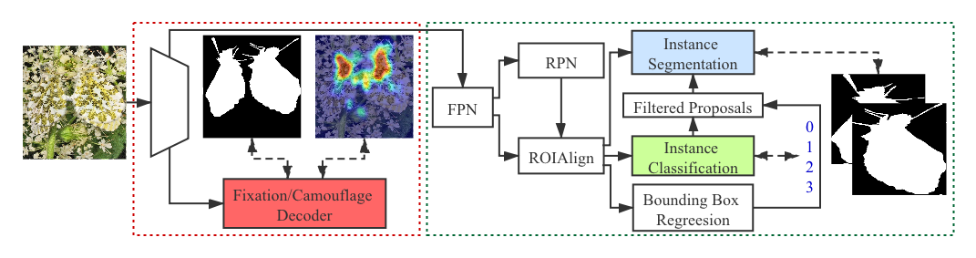
Figure 2: Overview of the proposed network. We have two main tasks in our framework, namely the camouflaged object ranking which is supervised by the ranking ground truth and each rank based binary segmentation map, and a joint learning framework for camouflaged object discriminative region localization and segmentation. With the input image, our model is trained end-to-end to produce discriminative region localization, camouflaged object segmentation and camouflage ranking. “FPN” and “RPN” are the Feature Pyramid Network [27] and the Region Proposal Network [37], respectively.

Camouflaged object detection: Camouflage is a useful technique for animals to conceal themselves from visual detection by others [32, 46]. In early research, most methods use low-level features, including texture, edge, brightness and color features, to discriminate objects from the background [3, 54, 45, 55, 25, 34]. However, these methods usually fell into the trap of camouflage, as the low-level features are often disrupted in camouflage to deceive the perceivers. Therefore, recent research usually resorts to the huge capacity of deep network to recognize the more complex properties of camouflage. Among those, Le et al.[22] introduced the joint image classification and camouflaged object segmentation framework. Yan et al.[56] presented an adversarial segmentation stream using a flipped image as input to enhance the discriminative ability of the main segmentation stream for camouflaged object detection. Fan et al.[10] proposed SINet to gradually locate and search for the camouflaged object. All of the above methods try to mimic the perception and cognition of observers performing on camouflaged objects. However, they ignored an important attribute: the time that observers spend on searching for the camouflaged object varies in a wide range and heavily depends on the effectiveness of camouflage [46]. Therefore, they fail to consider that the features employed to detect the objects are also different when they have different camouflage degrees, which is a useful indicator in camouflage research [35]. To reveal the degree of camouflage, and discover the regions that make camouflaged objects detectable, we introduce the first camouflaged object ranking method and camouflaged object discriminative region localization solution to effectively analyse the attribute of camouflage.

Ranking based dense prediction models: For some attributes, saliency, it’s natural to have ranking in the annotation for better understanding of the task. Islam et al.[2] argued that saliency is a relative concept when multiple observers are queried. Toward this, they collected a saliency ranking dataset based on the PASCAL-S dataset [26] with 850 images labeled by 12 observers. Based on this dataset, they designed an encoder-decoder model to predict saliency masks of different levels to achieve the final ranking prediction. Following their idea, Yildirim et al.[58] evaluated saliency ranking based on the assumption that objects in natural images are perceived to have varying levels of importance. Siris et al.[40] defined ranking by inferring the order of attention shift when people view an image. Their dataset is based on the fixation data provided by SALICON [18]. As far as we know, there exist no camouflaged object ranking models. Similar to saliency, camouflaged object have levels, and the camouflaged objects of higher level background matching or disruptive coloration may hide better in the environment, indicating a higher level of camouflage. Based on this, our ranking based solution leads to better understanding about evolution of animals. Different from saliency ranking, which is relative within a single image, we define camouflage ranking as relative and progressive across the entire dataset, which is generated based on the median fixation time of multiple observers.

Discriminative region localization technique: The discriminative regions [63] are those leading to accurate classification, , the head of the animals and . Zhou et al.[63] introduced the class activation map (CAM) to estimate the discriminative region of each class, which is the basis of many weakly supervised methods [1, 51, 17, 50, 24, 43, 47]. Selvaraju et al.[39] extended CAMs by utilizing the gradient of the class score w.r.t. activation of the last convolutional layer of CNN to investigate the importance of each neuron. Chattopadhay et al.[6] used a linear combination of positive gradients w.r.t. activation maps of the last convolutional layer to capture the importance of each class activation map for the final classification. Zhang et al.[61] erased the high activation area iteratively to force a CNN to learn all relevant features and therefore expanded the discriminative region. Similar to the existing discriminative region localization techniques, we introduce the first camouflaged object discriminative region localization method to reveal the most salient region of the camouflaged objects.

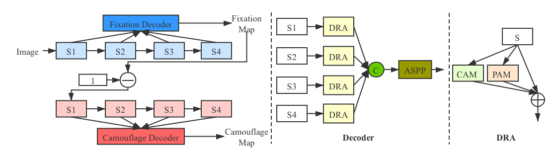
Figure 3: Overview of the joint fixation and segmentation prediction network. The first part indicates the pipeline that the Fixation Decoder and Camouflage Decoder generates the corresponding maps. The second part is the structrue of the decoders, where “ASPP” is the denseaspp module [57]. The third part is the structure of the dual residual attention module “DRA” in decoder, in which “CAM” and “PAM” are channel attention module and position attention module from [13].

3 Our Method

As there exists no localization or ranking based camouflage dataset, we will first discuss our new dataset, and then present our model.

3.1 The new dataset

Dataset collection: To achieve camouflaged object localization and ranking, we first relabel some images from existing camouflaged object detection datasets CAMO [22] and COD10K [10] to have both localization (fixation) annotation and ranking annotation. We denote the reprocessed dataset as CAM-FR. The basic assumption is that the longer it takes for the viewer to find the camouflaged object, the higher level of the camouflaged object [46]. Based on this, we record the detection delay for each camouflaged object, and use it as the indicator for camouflage ranking.

To do so, we use an eye tracker (SMI RED250) and record the time for each camouflaged object to be noticed. SMI RED250 provides three sampling rates, 60Hz, 120Hz and 250Hz, representing the accuracy of the recorded detection delay. We use the 250Hz sampling rate in our experiment. The operating distance is 60-80cm, which is the distance from observers to the camouflaged image. The movement range is 40cm in the horizontal direction and 20cm in the vertical direction, which is the range for the observers to move in order to discover the camouflaged objects.

With the existing camouflaged object detection training datasets, , the COD10K [10] and CAMO datasets [22], we invite six observers to view each image with the task of camouflaged object detection. We define the median observation time across different observers as the detection delay for each camouflaged instance, with the help of instance-level annotations. Specifically, we define the observation time for the $j$-th observer towards the $i$-th instance as:

$$\triangle t_{ij}=\mathrm{median}(\boldsymbol{\delta t_{ij}}),\ \boldsymbol{\delta t_{ij}}=\{t_{ij}^{k}-t_{j}^{0}\}_{k=1}^{K}$$ (1)

$K$ is the number of fixation points on the instance, $t_{j}^{0}$ is the start time for observer $j$ to watch the image and $t_{ij}^{k}$ is the time of the $k$-th fixation point on the instance $i$ with observer $j$. To avoid the influence of extreme high or low fixation time, we use the median instead of the mean value:

$$\mathrm{median}(\boldsymbol{x})=\left\{\begin{array}[]{cc}x_{(n+1)/2},&\mathrm{n}/2\neq 0\\ \frac{x_{\lfloor{n/2\rfloor}}+x_{\lfloor{n/2\rfloor}+1}}{2},&\mathrm{n}/2=0\end{array}\right.$$ (2)

in which $\boldsymbol{x}=\{x_{l}\}_{l=1}^{n}$ is a set indexed in ascending order. Considering different perception ability of observers, we define the final detection delay for instance $i$ as the median across the six observers: $\triangle t_{i}=\mathrm{median}_{j}(\triangle t_{ij})$, which is then used to get our ranking dataset.

There exist two different cases that may result into no fixation points in the camouflaged instance region. The first is caused by a mechanical error of the eye tracker or incorrect operation by observers. The second is caused by the higher level of camouflage, which makes it difficult to detect the camouflaged object. We set a threshold to distinguish these two situations. If more than half of the observers ignore the instance, we consider it as a hard sample and the search time is set to 1 (after normalization). Otherwise, values of the corresponding observers are deleted and the median is computed from the remaining detection decays.

Dataset information: Our dataset CAM-FR contains 2,000 images for training and 280 images for testing. The training set includes 1,711 images from the COD10K-CAM training set [10] and 289 images are from the CAMO training set [22]. Then, we relabel 238 images from the COD10K-CAM training set and 42 images from the CAMO training set as the testing set. In CAM-FR, we have different ranks (rank 0 is the background), where rank 1 is the hardest level, rank 2 is median and rank 3 is the easiest level.

Model design with the new dataset: Based on our new dataset, we propose to simultaneously localize, segment and rank the camouflaged objects. Given an input image, the first two tasks regress the fixation map and segmentation map respectively, while the third task involves instance segmentation (camouflaged object detection) and classification (camouflaged object ranking). We build the three tasks within one unified framework as shown in Fig. 2, where the localization network and segmentation network are integrated in one joint learning framework. The ranking model shares the backbone network with the joint learning framework to produce camouflage ranking.

3.2 Joint localization and segmentation

Task analysis: We define the “discriminative region” as a region that makes the camouflaged object apparent. Compared with other regions of the camouflaged object, the discriminative region should have a higher contrast with it’s surroundings than the other regions of the camouflaged object. Based on this observation, we design a reverse attention module based joint camouflaged object discriminative region localization and segmentation network in Fig. 3, which can simultaneously regress the discriminative regions that make the camouflaged objects obvious and segment the camouflaged objects.

Network design: We built our joint learning framework with ResNet50 [16] as backbone shown in Fig. 3. Given an input image $I$, we feed it to the backbone to obtain feature representation $s_{1},s_{2},s_{3},s_{4}$, representing feature maps from different stages of the backbone network. Similar to existing ResNet50 based networks, we define a group of convolutional layers that produce the same spatial size as belonging to the same stage of the network. Then we design the “Fixation Decoder” and “Camouflage Decoder” modules with the same network structure, as “Decoder” in Fig. 3, to regress the fixation map and segmentation map respectively. Each $s_{i}$, $i=1,...,4$ is fed to a convolutional layer of kernel size $3\times 3$ to achieve the new feature map $\{s_{i}^{\prime}\}_{i=1}^{4}$ of channel dimension $C=32$ respectively. Then, we propose the dual residual attention model as “DRA” in Fig. 3 by modifying the dual attention module [13], to obtain a discriminative feature representation with a position attention module (PAM) and channel attention module (CAM). The “ASPP” in the decoder is the denseaspp module in [57] to achieve a multi-scale receptive field.

With the proposed “Fixation Decoder” module, we obtain our discriminative region, which will be compared with the provided ground truth fixation map to produce our loss function for the fixation branch. Then, based on our observation that the fixated region usually has higher saliency than the other parts of the object, we introduce a reverse attention based framework to jointly learn the discriminative region and regress the whole camouflaged object. Specifically, given the discriminative region prediction $F$, we obtain the reverse attention as $1-F$. Then we treat it as the attention and multiply it with the backbone feature $s_{1}$ to generate the reverse attention guided feature $\{s_{i}^{r}\}_{i=1}^{4}$ similar to [52]. Then, we have the “Camouflage Decoder” to generate our saliency prediction $S$ from $\{s_{i}^{r}\}_{i=1}^{4}$.

Objective function: We have two loss functions in the joint learning framework: the discriminative region localization loss and the camouflaged object detection loss. For the former, we use the binary cross-entropy loss $\mathcal{L}_{f}$. For the latter, we adopt the pixel position aware loss as in [49] to produce predictions with higher structure accuracy. Then we define our joint learning framework based loss function as:

$$\mathcal{L}_{fc}=\mathcal{L}_{f}+\lambda\mathcal{L}_{c},$$ (3)

where $\lambda$ is a weight to measure the importance of each task, and empirically we set $\lambda=1$ in this paper.

3.3 Inferring the ranks of camouflaged objects

Instance segmentation based rank model: We construct our camouflage ranking model on the basis of Mask R-CNN [15] to learn the degree of camouflage. Similar to the goal of Mask R-CNN [15], the aim of the camouflage ranking model is jointly segmenting the camouflaged objects and inferring their ranks. Following the standard pipeline of Mask R-CNN, we design a camouflaged object ranking model as shown in Fig. 2, with the “Instance Segmentation” branch supervised by the binary ground truth of each camouflaged instance, and an “Instance Classification” branch to produce the camouflaged object ranking.

Firstly, we feed the image $I\in\mathbb{R}^{h\times w\times 3}$ into the backbone network (ResNet50 [16] in particular) to extract image features. Then the “Feature Pyramid Network” (FPN) [27] is employed to integrate the feature maps of different levels. The final set of feature maps is denoted as $P=\{P_{1},\cdots,P_{n}\}$, where $n$ is the number of layers. Then the “Region Proposal Network” (RPN) [37] is adopted, which takes the feature of the whole image as input, and detects the regions that are likely to contain the camouflaged instances, the regions of interest (ROIs). Two branches are included in RPN: 1) a classification branch, which determines whether the candidate bounding box contains the camouflaged object; and 2) a regression branch, which regresses the coordinates of the ground truth camouflaged object bounding box.

With features produced by FPN, the ROIAlign module [15] is used to extract feature maps of the ROIs. Then, we predict the rank and regress the location of the camouflaged object, respectively. Finally, features of the detected camouflaged object are fed into a segmentation branch to output a binary mask for each camouflaged instance.

During training, a multi-task loss with three components is minimized:

$$\mathcal{L}=\mathcal{L}_{rpn}+\mathcal{L}_{rank}+\mathcal{L}_{mask},$$ (4)

where $\mathcal{L}_{rpn}$ is to train the RPN, $\mathcal{L}_{rank}$ is the loss for the ranking model, and $\mathcal{L}_{mask}$ is only defined on the region where the prediction of rank is not 0 (background) and allows the network to segment instances of each rank. Both $\mathcal{L}_{rpn}$ and $\mathcal{L}_{rank}$ consist of classification loss and regression loss. For RPN, it aims to check the existence of the camouflaged instance in the proposal and regress its location. For the rank model, it infers the rank of camouflage and regresses object location.

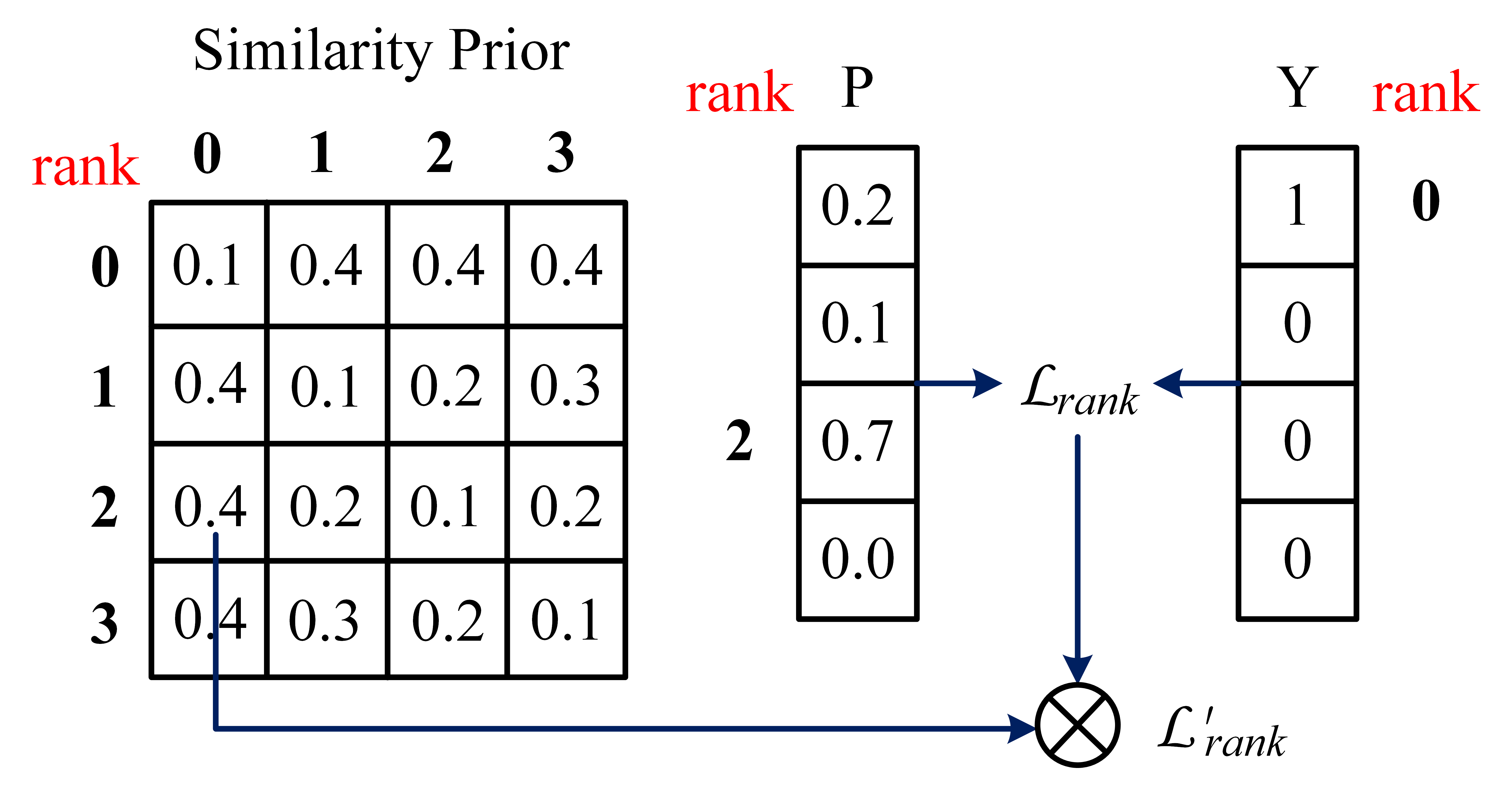
Figure 4: Label similarity as a prior to consider the rank label dependency of our ranking dataset. $\mathrm{P}$ and $\mathrm{Y}$ denote the prediction and the one-hot ground truth, respectively.

Label similarity as prior: Directly inferring ranks of camouflage with Mask-RCNN may produce unsatisfactory results due to the independence of labels in the instance segmentation dataset. However, in our ranking scenario, the ranks are progressive, camouflaged object of rank 3 (the easiest level) is easier to notice than rank 2 (the median). Moreover, the instance of rank 1 should be penalized more if it’s misclassified as rank 3 instead of rank 2. Towards this, we intend to employ such a constraint on $\mathcal{L}_{rank}$ in Eq. 4. Specifically, we define a camouflaged instance similarity prior $S_{p}$, which is a $4\times 4$ matrix as shown in Fig. 4, with each $S_{p}(m,n)$ representing the penalty for predicting rank $n$ as rank $m$. Given the prediction of the instance classification network in Fig. 2, and the ground truth instance rank, we first compute the original rank loss $\mathcal{L}_{rank}$ (before we compute the mean of $\mathcal{L}_{rank}$). Then, we weight it with the specific similarity prior $S_{p}(m,n)$. As is illustrated in Fig. 4, the predicted rank is 2, and the ground truth rank is 0, then we get penalty $S_{p}(2,0)=0.4$, and multiply it with the original rank loss $\mathcal{L}_{rank}$ to obtain the weighted loss $\mathcal{L}^{\prime}_{rank}$. Although we pay more attention to misclassified samples, a weight should be assigned to the loss of correct samples, making them produce more confident scores.

Table 1: Performance of baseline models trained with our CAM-FR dataset on benchmark testing sets.

	CAMO				CHAMELEON				COD10K				NC4K
Method	$S_{\alpha}\uparrow$	$F^{\mathrm{mean}}_{\beta}\uparrow$	$E^{\mathrm{mean}}_{\xi}\uparrow$	$\mathcal{M}\downarrow$	$S_{\alpha}\uparrow$	$F^{\mathrm{mean}}_{\beta}\uparrow$	$E^{\mathrm{mean}}_{\xi}\uparrow$	$\mathcal{M}\downarrow$	$S_{\alpha}\uparrow$	$F^{\mathrm{mean}}_{\beta}\uparrow$	$E^{\mathrm{mean}}_{\xi}\uparrow$	$\mathcal{M}\downarrow$	$S_{\alpha}\uparrow$	$F^{\mathrm{mean}}_{\beta}\uparrow$	$E^{\mathrm{mean}}_{\xi}\uparrow$	$\mathcal{M}\downarrow$
SCRN [53]	0.702	0.632	0.731	0.106	0.822	0.726	0.833	0.060	0.756	0.623	0.793	0.052	0.793	0.729	0.823	0.068
CSNet[14]	0.704	0.633	0.753	0.106	0.819	0.759	0.859	0.051	0.745	0.615	0.808	0.048	0.785	0.729	0.834	0.065
UCNet [59]	0.703	0.640	0.740	0.107	0.833	0.781	0.890	0.049	0.756	0.650	0.823	0.047	0.792	0.751	0.854	0.065
BASNet [36]	0.644	0.578	0.588	0.143	0.761	0.657	0.797	0.080	0.640	0.579	0.713	0.072	0.724	0.648	0.780	0.089
SINet [10]	0.697	0.579	0.693	0.130	0.820	0.731	0.835	0.069	0.733	0.588	0.768	0.069	0.779	0.696	0.800	0.086
Ours_cod_new	0.708	0.645	0.755	0.105	0.842	0.794	0.896	0.046	0.760	0.658	0.831	0.045	0.797	0.758	0.854	0.061

4 Experimental Results

4.1 Setup

Dataset: We train our framework with CAM-FR training set to provide a baseline to simultaneously achieve camouflaged object detection (Ours_cod_new), discriminative region localization (Ours_fix_new) and camouflage ranking (Ours_rank_new) and test on the testing set of CAM-FR. Further, to compare our performance with benchmark models, we further train a single camouflaged object detection model (Ours_cod_full) with the conventional training dataset which contains 3,040 images from COD10K and 1,000 images from CAMO, and test on the existing testing datasets, including CAMO [22], COD10K [10], CHAMELEMON [42] and our NC4K testing dataset.

Training details: A pretrained ResNet50 [16] is employed as our backbone network. During training, the input image is resized to $352\times 352$. Candidate bounding boxes spanning three scales (4, 8, 16) and three aspect ratios (0.5, 1.0, 2.0) are selected from each pixel. In the RPN module of the ranking model, the IoU threshold with the ground truth is set to 0.7, which is used to determine whether the candidate bounding box is positive (IoU$>$0.7) or negative (IoU$<$0.7) in the next detection phase. The IoU threshold is set to 0.5 to determine whether the camouflaged instances are detected and only positive ones are sent into the segmentation branch. Our model in Fig. 2 is trained on one GPU (Nvidia RTX 1080 Ti) for 10k iterations (14 hours) with a mini-batch of 10 images, using the Adam optimizer with a learning rate of 5e-5.

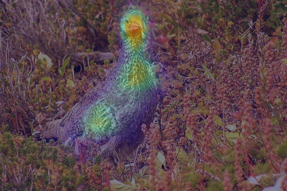
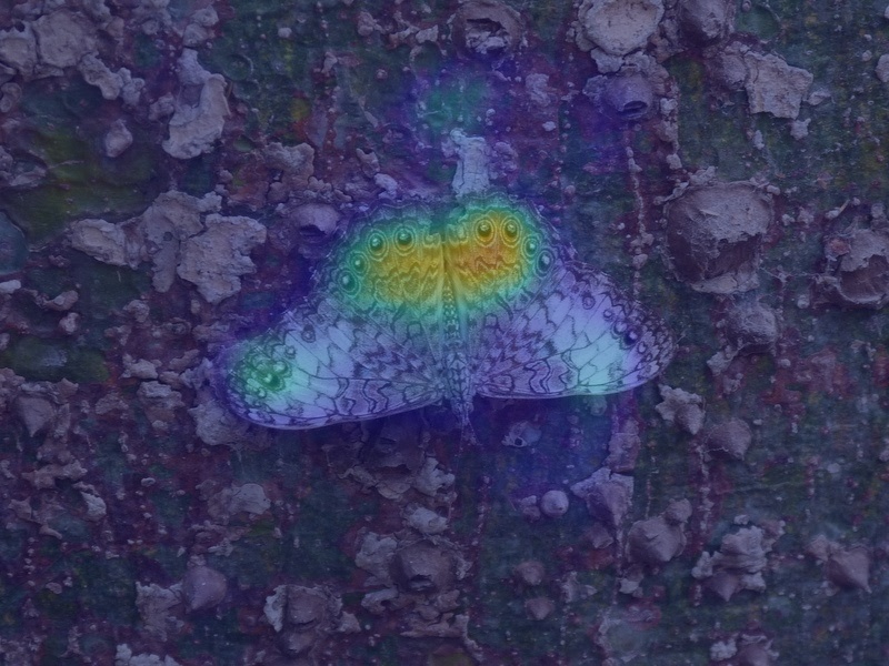
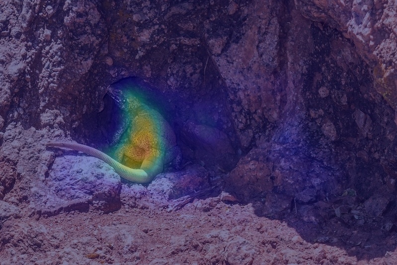
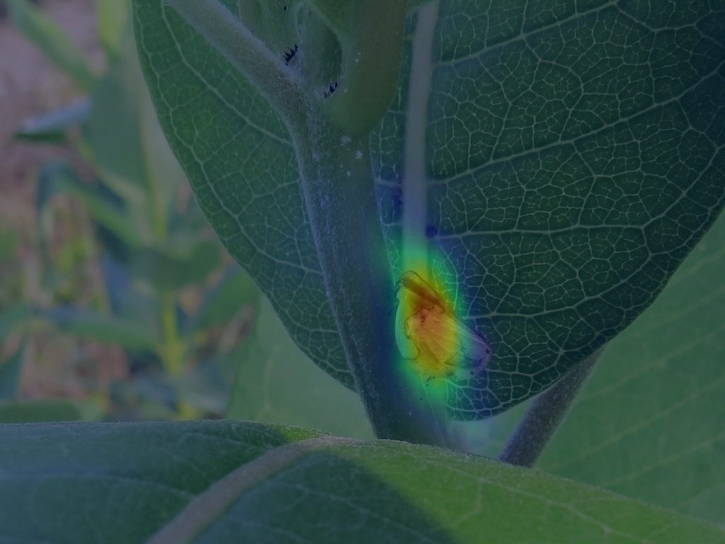
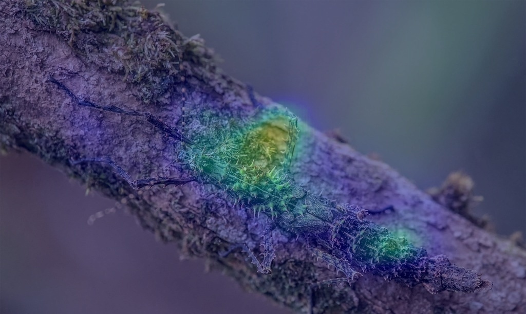
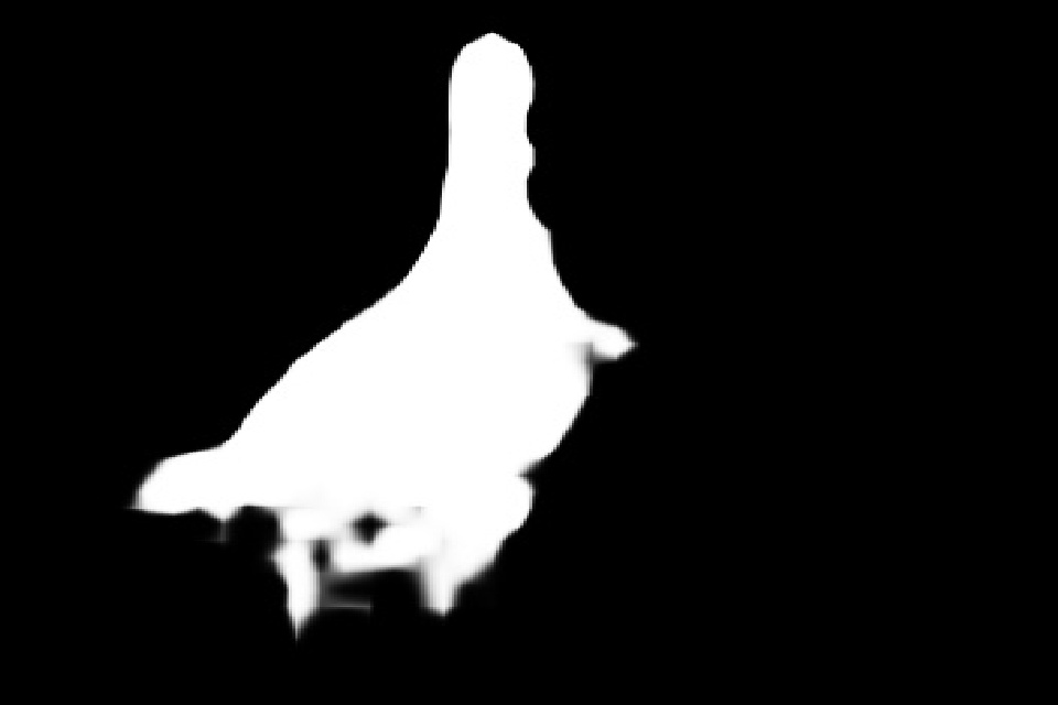
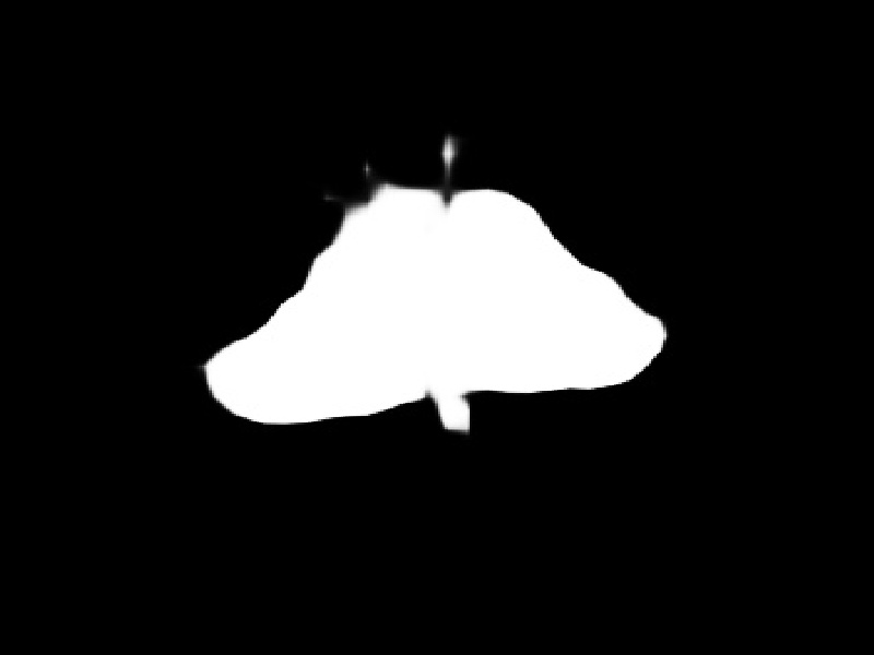
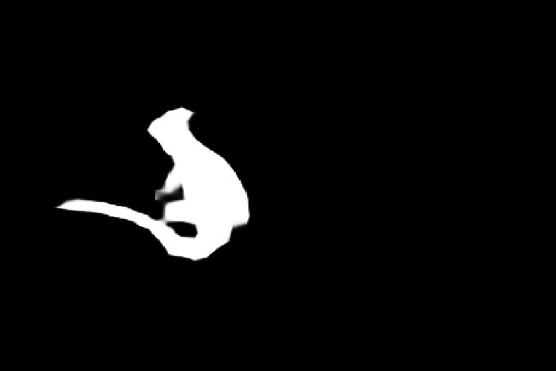
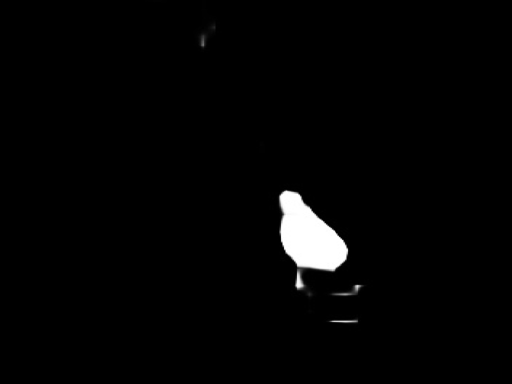
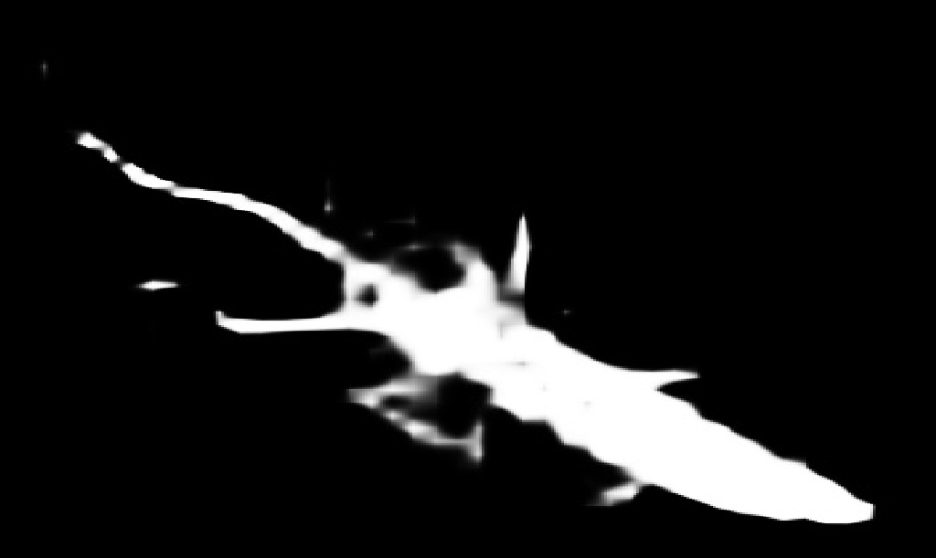
Figure 5: Visual performance of the proposed algorithm. From top to bottom: fixation, camouflaged object detection and ranking predictions. The green, orange and blue annotations in the third row indicate camouflage rank 3 (easiest), 2 (median) and 1 (hardest), respectively.

Evaluation metrics: Conventionally, camouflaged object detection is defined as a binary segmentation task, and the widely used evaluation metrics include Mean Absolute Error, Mean F-measure, Mean E-measure [9] and S-measure [7] denoted as $\mathcal{M}$, $F_{\beta}^{\mathrm{mean}}$, $E_{\xi}^{\mathrm{mean}}$, $S_{\alpha}$, respectively.

We find that the above four evaluation metrics cannot evaluate the performance of ranking based prediction. For the ranking task, [2] introduced the Salient Object Ranking (SOR) metric to measure ranking performance, which is defined as the Spearman’s Rank-Order Correlation between the ground truth rank order and the predicted rank order of salient objects. However, it cannot be used in our scenario, as Spearman’s Rank-Order Correlation is based on at least two different ranking levels. However, in our ranking based dataset, most of the images have only one camouflaged object. To deal with this, we introduce $r_{MAE}$:

$$r_{MAE}=\frac{\sum_{i=1}^{w}\sum_{j=1}^{h}|r_{ij}-\hat{r}_{ij}|}{N},$$ (5)

where $N$ is the number of pixels, $w$ and $h$ are the width and height of the image. $\hat{r}_{ij}$ and $r_{ij}$ are the predicted and ground truth ranks respectively with values $0,1,2,3$ corresponding to “background”, “hardest”, “median” and “easiest”, respectively. If the prediction is consistent with the ground truth, their difference is supposed to be 0. In $r_{MAE}$, an “easiest” sample is punished less when it is predicted as a “median” sample than as a “hardest” sample. Accordingly, it is a convincing metric to evaluate the performance of ranking. For the discriminative region localization, we adopt the widely used fixation prediction evaluation metrics including Similarity ($SIM$) [19], Linear Correlation Coefficient ($CC$) [23], Earth Mover’s Distance ($EMD$) [38], Kullback–Leibler Divergence ($KLD$) [21], Normalized Scanpath Saliency ($NSS$) [33], AUC_Judd ($AUC\_J$) [20], AUC_Borij ($AUC\_B$)[5], shuffled AUC ($sAUC$) [4] as shown in Table 2.

Table 2: Performance of the discriminative region localization.

$SIM\uparrow$	$CC\uparrow$	$EMD\downarrow$	$KLD\downarrow$	$NSS\uparrow$	$AUC\_J\uparrow$	$AUC\_B\uparrow$	$sAUC\uparrow$
0.622	0.776	3.361	0.995	2.608	0.901	0.844	0.658

Table 3: Comparison of camouflage ranking methods.

Method	$MAE$	$r_{MAE}$
Ours_rank_new	0.049	0.139
SOLOv2[48]	0.049	0.210
MS-RCNN[30]	0.053	0.142
RSDNet[2]	0.074	0.293

Table 4: Performance comparison with baseline models on benchmark dataset and our NC4K dataset.

	CAMO				CHAMELEON				COD10K				NC4K
Method	$S_{\alpha}\uparrow$	$F_{\beta}^{\mathrm{mean}}\uparrow$	$E_{\xi}^{\mathrm{mean}}\uparrow$	$\mathcal{M}\downarrow$	$S_{\alpha}\uparrow$	$F_{\beta}^{\mathrm{mean}}\uparrow$	$E_{\xi}^{\mathrm{mean}}\uparrow$	$\mathcal{M}\downarrow$	$S_{\alpha}\uparrow$	$F_{\beta}^{\mathrm{mean}}\uparrow$	$E_{\xi}^{\mathrm{mean}}\uparrow$	$\mathcal{M}\downarrow$	$S_{\alpha}\uparrow$	$F_{\beta}^{\mathbf{\mathrm{mean}}}\uparrow$	$E_{\xi}^{\mathbf{\mathrm{mean}}}\uparrow$	$\mathcal{M}\downarrow$
PiCANet[29]	0.701	0.573	0.716	0.125	0.765	0.618	0.779	0.085	0.696	0.489	0.712	0.081	0.758	0.639	0.773	0.088
CPD [52]	0.716	0.618	0.723	0.113	0.857	0.771	0.874	0.048	0.750	0.595	0.776	0.053	0.790	0.708	0.810	0.071
SCRN [53]	0.779	0.705	0.796	0.090	0.876	0.787	0.889	0.042	0.789	0.651	0.817	0.047	0.832	0.759	0.855	0.059
CSNet[14]	0.771	0.705	0.795	0.092	0.856	0.766	0.869	0.047	0.778	0.635	0.810	0.047	0.819	0.748	0.845	0.061
PoolNet [28]	0.730	0.643	0.746	0.105	0.845	0.749	0.864	0.054	0.740	0.576	0.776	0.056	0.785	0.699	0.814	0.073
UCNet [59]	0.739	0.700	0.787	0.094	0.880	0.836	0.930	0.036	0.776	0.681	0.857	0.042	0.813	0.777	0.872	0.055
F3Net [49]	0.711	0.616	0.741	0.109	0.848	0.770	0.894	0.047	0.739	0.593	0.795	0.051	0.782	0.706	0.825	0.069
ITSD[64]	0.750	0.663	0.779	0.102	0.814	0.705	0.844	0.057	0.767	0.615	0.808	0.051	0.811	0.729	0.845	0.064
BASNet [36]	0.615	0.503	0.671	0.124	0.847	0.795	0.883	0.044	0.661	0.486	0.729	0.071	0.698	0.613	0.761	0.094
NLDF[31]	0.665	0.564	0.664	0.123	0.798	0.714	0.809	0.063	0.701	0.539	0.709	0.059	0.738	0.657	0.748	0.083
EGNet [62]	0.737	0.655	0.758	0.102	0.856	0.766	0.883	0.049	0.751	0.595	0.793	0.053	0.796	0.718	0.830	0.067
SSAL[60]	0.644	0.579	0.721	0.126	0.757	0.702	0.849	0.071	0.668	0.527	0.768	0.066	0.699	0.647	0.778	0.092
SINet [10]	0.745	0.702	0.804	0.092	0.872	0.827	0.936	0.034	0.776	0.679	0.864	0.043	0.810	0.772	0.873	0.057
Ours_cod_full	0.793	0.725	0.826	0.085	0.893	0.839	0.938	0.033	0.793	0.685	0.868	0.041	0.839	0.779	0.883	0.053

Table 5: Ablation experiments of the proposed model.

	Metrics for FIX								Metrics for COD				Metrics for Ranking
Model	$SIM\uparrow$	$CC\uparrow$	$EMD\downarrow$	$KLD\downarrow$	$NSS\uparrow$	$AUC\_J\uparrow$	$AUC\_B\uparrow$	$sAUC\uparrow$	$S_{\alpha}\uparrow$	$F^{\mathrm{mean}}_{\beta}\uparrow$	$E^{\mathrm{mean}}_{\xi}\uparrow$	$\mathcal{M}\downarrow$	$MAE\downarrow$	$r_{MAE}\downarrow$
FIX	0.619	0.765	3.398	1.457	2.567	0.892	0.842	0.644	‡	‡	‡	‡	‡	‡
COD	‡	‡	‡	‡	‡	‡	‡	‡	0.723	0.542	0.808	0.052	‡	‡
Ranking	‡	‡	‡	‡	‡	‡	‡	‡	‡	‡	‡	‡	0.046	0.143
Ours	0.622	0.776	3.398	0.995	2.608	0.901	0.844	0.658	0.756	0.594	0.824	0.045	0.049	0.139

Competing methods: As the number of the competing methods (SINet [10] is the only deep model with code and camouflage maps available) is too limited, and considering the similarity of salient object detection and camouflaged object detection, we re-train state-of-the-art salient object detection models on the camouflaged object detection dataset [10], and treat them as competing methods. As there exist no camouflaged object ranking models, we then implement three rank or instance based object segmentation methods for camouflage rank estimation, including RSDNet [2] for salient ranking prediction, SOLOv2 [48] and Mask Scoring-RCNN (MS-RCNN) [30] for instance segmentation. For the discriminative region localization task, we provide baseline performance.

4.2 Performance comparison

Discriminative region localization: We show the discriminative region of camouflaged objects in the first row of Fig. 5, which indicates that the discriminative region, heads of animals and salient patterns, could be correctly identified. Furthermore, we show the baseline performance in Table 2 to quantitatively evaluate our method.

Camouflaged object detection: We show the camouflaged detection map in the second row of Fig. 5, which is trained using our ranking dataset. We further show the quantitative results in Table 1, where the competing methods are re-trained using our ranking dataset. Our results in both Fig. 5 and Table 1 illustrate the effectiveness of our solution. Moreover, as the only code-available camouflaged model, SINet [10], is trained with 4,040 images from COD10K [10] and CAMO [22], for a fair comparison, we also train our camouflaged object detection branch with the 4,040 images, and show performance in Table 4, which further illustrates effectiveness of our method.

Camouflaged object ranking: We show the ranking prediction in the third row of Fig. 5. The stacked representation of the ground truth in RSDNet is designed specifically for salient objects. We rearrange the stacked masks based on the assumption that the higher degree of camouflage corresponds to the lower degree of saliency. As is shown in Table 3, the performance of MS-RCNN is inferior to our method in both $MAE$ and $r_{MAE}$. Besides, although SOLOv2 achieves comparable performance with ours in terms of $MAE$, its ranking performance in $r_{MAE}$ is far from satisfactory. In order to determine the saliency rank, RSDNet borrows the instance-level ground truth to compute and descend average saliency scores of instances in an image. Therefore, the ranking is unavailable if there exists no instance-level ground truth. While analysing the model setting and performance in Table 3, we clear observe the superior performance of the ranking model we proposed.

4.3 Ablation Study

We integrate three different tasks in our framework to achieve simultaneous discriminative region localization, camouflaged object detection and camouflaged object ranking. We then train them separately on the ranking dataset to further evaluate our solution, and show the performance on our ranking testing set in Table 5. Since the experiment for each task does not have values on metrics for the other two tasks, we use ${\ddagger}$ to denote that the value is unavailable. For the discriminative region localization model (“FIX”), we keep the backbone network with the “Fixation Decoder” in Fig. 3. For the camouflaged object detection model (“COD”), as illustrated above, we keep the backbone network with the “Camouflage Decoder”. For the ranking model, we remove the “Joint Fixation and Segmentation prediction” module in Fig. 2, and train the camouflaged object ranking network alone with the ranking annotation.

In Table 5, “Ours” is achieved through jointly training the three tasks. Comparing “FIX” and “COD” with “Ours”, we observe consistently better performance of the joint fixation baseline and our joint camouflaged prediction, which explains the effectiveness of the joint learning framework. While, we observe similar performance of the ranking based solution alone (“Ranking” in Table 5) compared with our joint learning ranking performance (“Ours” in Table 5), which indicates that the ranking model benefits less from the other two tasks in our framework.

Further, we adopt the dual residual attention modules (DRA) [13] in our framework as shown in Fig. 3 to provide both global context information and dircriminative feature representation. We then remove the DRA modules from our triple task learning framework, and observe slightly decreased performance. The main reason is that camouflaged object detection is context-based, and the effective modelling of object context information is very beneficial.

5 Conclusion

We introduce two new tasks for camouflaged object detection, namely camouflaged object discriminative region localization and camouflaged object ranking, along with relabeled corresponding datasets. The former aims to find the discriminative regions that make the camouflaged object detectable, while the latter tries to explain the level of camouflage. We built our network in a joint learning framework to simultaneously localize, segment and rank the camouflaged objects. Experimental results show that our proposed joint learning framework can achieve state-of-the-art performance. Furthermore, the produced discriminative region and rank map provide insights toward understanding the nature of camouflage. Moreover, our new testing dataset NC4K can better evaluate the generalization ability of the camouflaged object detection models.

References

- [1] Jiwoon Ahn and Suha Kwak. Learning pixel-level semantic affinity with image-level supervision for weakly supervised semantic segmentation. In IEEE Conf. Comput. Vis. Pattern Recog., pages 4981–4990, 2018.
- [2] Md Amirul Islam, Mahmoud Kalash, and Neil DB Bruce. Revisiting salient object detection: Simultaneous detection, ranking, and subitizing of multiple salient objects. In IEEE Conf. Comput. Vis. Pattern Recog., pages 7142–7150, 2018.
- [3] Nagappa U Bhajantri and P Nagabhushan. Camouflage defect identification: a novel approach. In International Conference on Information Technology (ICIT), pages 145–148. IEEE, 2006.
- [4] Ali Borji, Dicky N Sihite, and Laurent Itti. Quantitative analysis of human-model agreement in visual saliency modeling: A comparative study. IEEE T. Image Process., 22(1):55–69, 2012.
- [5] Ali Borji, Hamed R Tavakoli, Dicky N Sihite, and Laurent Itti. Analysis of scores, datasets, and models in visual saliency prediction. In Int. Conf. Comput. Vis., pages 921–928, 2013.
- [6] Aditya Chattopadhay, Anirban Sarkar, Prantik Howlader, and Vineeth N Balasubramanian. Grad-cam++: Generalized gradient-based visual explanations for deep convolutional networks. In Proc. IEEE Winter Conf. on App. of Comp. Vis., pages 839–847. IEEE, 2018.
- [7] Deng-Ping Fan, Ming-Ming Cheng, Yun Liu, Tao Li, and Ali Borji. Structure-measure: A new way to evaluate foreground maps. In Int. Conf. Comput. Vis., pages 4548–4557, 2017.
- [8] Deng-Ping Fan, Ge-Peng Ji, Ming-Ming Cheng, and Ling Shao. Concealed object detection. arXiv preprint arXiv:2102.10274, 2021.
- [9] Deng-Ping Fan, Ge-Peng Ji, Xuebin Qin, and Ming-Ming Cheng. Cognitive vision inspired object segmentation metric and loss function. SCIENTIA SINICA Informationis, 2021.
- [10] Deng-Ping Fan, Ge-Peng Ji, Guolei Sun, Ming-Ming Cheng, Jianbing Shen, and Ling Shao. Camouflaged object detection. In IEEE Conf. Comput. Vis. Pattern Recog., pages 2777–2787, 2020.
- [11] Deng-Ping Fan, Ge-Peng Ji, Tao Zhou, Geng Chen, Huazhu Fu, Jianbing Shen, and Ling Shao. Pranet: Parallel reverse attention network for polyp segmentation. In International Conference on Medical Image Computing and Computer-Assisted Intervention, pages 263–273. Springer, 2020.
- [12] Deng-Ping Fan, Tao Zhou, Ge-Peng Ji, Yi Zhou, Geng Chen, Huazhu Fu, Jianbing Shen, and Ling Shao. Inf-net: Automatic covid-19 lung infection segmentation from ct images. IEEE Trans. Med. Imaging, 39(8):2626–2637, 2020.
- [13] Jun Fu, Jing Liu, Haijie Tian, Yong Li, Yongjun Bao, Zhiwei Fang, and Hanqing Lu. Dual attention network for scene segmentation. In IEEE Conf. Comput. Vis. Pattern Recog., pages 3146–3154, 2019.
- [14] Shang-Hua Gao, Yong-Qiang Tan, Ming-Ming Cheng, Chengze Lu, Yunpeng Chen, and Shuicheng Yan. Highly efficient salient object detection with 100k parameters. In Eur. Conf. Comput. Vis., 2020.
- [15] Kaiming He, Georgia Gkioxari, Piotr Dollár, and Ross Girshick. Mask r-cnn. In Int. Conf. Comput. Vis., pages 2961–2969, 2017.
- [16] Kaiming He, Xiangyu Zhang, Shaoqing Ren, and Jian Sun. Deep residual learning for image recognition. In IEEE Conf. Comput. Vis. Pattern Recog., pages 770–778, 2016.
- [17] Zilong Huang, Xinggang Wang, Jiasi Wang, Wenyu Liu, and Jingdong Wang. Weakly-supervised semantic segmentation network with deep seeded region growing. In IEEE Conf. Comput. Vis. Pattern Recog., pages 7014–7023, 2018.
- [18] Ming Jiang, Shengsheng Huang, Juanyong Duan, and Qi Zhao. Salicon: Saliency in context. In IEEE Conf. Comput. Vis. Pattern Recog., pages 1072–1080, 2015.
- [19] Tilke Judd, Frédo Durand, and Antonio Torralba. A benchmark of computational models of saliency to predict human fixations. MIT tech report, Tech. Rep., 2012.
- [20] Tilke Judd, Krista Ehinger, Frédo Durand, and Antonio Torralba. Learning to predict where humans look. In Int. Conf. Comput. Vis., pages 2106–2113, 2009.
- [21] Solomon Kullback and Richard A Leibler. On information and sufficiency. The annals of mathematical statistics, 22(1):79–86, 1951.
- [22] Trung-Nghia Le, Tam V Nguyen, Zhongliang Nie, Minh-Triet Tran, and Akihiro Sugimoto. Anabranch network for camouflaged object segmentation. Comput. Vis. Image Unders., 184:45–56, 2019.
- [23] Olivier Le Meur, Patrick Le Callet, and Dominique Barba. Predicting visual fixations on video based on low-level visual features. Vision research, 47(19):2483–2498, 2007.
- [24] Jungbeom Lee, Eunji Kim, Sungmin Lee, Jangho Lee, and Sungroh Yoon. Ficklenet: Weakly and semi-supervised semantic image segmentation using stochastic inference. In IEEE Conf. Comput. Vis. Pattern Recog., pages 5267–5276, 2019.
- [25] Shuai Li, Dinei Florencio, Yaqin Zhao, Chris Cook, and Wanqing Li. Foreground detection in camouflaged scenes. In IEEE Int. Conf. Image Process., pages 4247–4251. IEEE, 2017.
- [26] Yin Li, Xiaodi Hou, Christof Koch, James M Rehg, and Alan L Yuille. The secrets of salient object segmentation. In IEEE Conf. Comput. Vis. Pattern Recog., pages 280–287, 2014.
- [27] Tsung-Yi Lin, Piotr Dollár, Ross Girshick, Kaiming He, Bharath Hariharan, and Serge Belongie. Feature pyramid networks for object detection. In IEEE Conf. Comput. Vis. Pattern Recog., pages 936–944, 2017.
- [28] Jiang-Jiang Liu, Qibin Hou, Ming-Ming Cheng, Jiashi Feng, and Jianmin Jiang. A simple pooling-based design for real-time salient object detection. In IEEE Conf. Comput. Vis. Pattern Recog., pages 3917–3926, 2019.
- [29] Nian Liu, Junwei Han, and Ming-Hsuan Yang. Picanet: Learning pixel-wise contextual attention for saliency detection. In IEEE Conf. Comput. Vis. Pattern Recog., pages 3089–3098, 2018.
- [30] Shu Liu, Lu Qi, Haifang Qin, Jianping Shi, and Jiaya Jia. Path aggregation network for instance segmentation. In IEEE Conf. Comput. Vis. Pattern Recog., pages 8759–8768, 2018.
- [31] Zhiming Luo, Akshaya Mishra, Andrew Achkar, Justin Eichel, Shaozi Li, and Pierre-Marc Jodoin. Non-local deep features for salient object detection. In IEEE Conf. Comput. Vis. Pattern Recog., pages 6609–6617, 2017.
- [32] Sami Merilaita, Nicholas E Scott-Samuel, and Innes C Cuthill. How camouflage works. Philosophical Transactions of the Royal Society B: Biological Sciences, 372(1724):20160341, 2017.
- [33] Robert J Peters, Asha Iyer, Laurent Itti, and Christof Koch. Components of bottom-up gaze allocation in natural images. Vision research, 45(18):2397–2416, 2005.
- [34] Thomas W Pike. Quantifying camouflage and conspicuousness using visual salience. Methods in Ecology and Evolution, 9(8):1883–1895, 2018.
- [35] Tasha Price, Samuel Green, Jolyon Troscianko, Tom Tregenza, and Martin Stevens. Background matching and disruptive coloration as habitat-specific strategies for camouflage. Scientific Reports, 9, 12 2019.
- [36] Xuebin Qin, Zichen Zhang, Chenyang Huang, Chao Gao, Masood Dehghan, and Martin Jagersand. Basnet: Boundary-aware salient object detection. In IEEE Conf. Comput. Vis. Pattern Recog., pages 7479–7489, 2019.
- [37] Shaoqing Ren, Kaiming He, Ross Girshick, and Jian Sun. Faster r-cnn: Towards real-time object detection with region proposal networks. In C. Cortes, N. Lawrence, D. Lee, M. Sugiyama, and R. Garnett, editors, Advances in Neural Information Processing Systems, volume 28, pages 91–99. Curran Associates, Inc., 2015.
- [38] Yossi Rubner, Carlo Tomasi, and Leonidas J Guibas. The earth mover’s distance as a metric for image retrieval. Int. J. Comput. Vis., 40(2):99–121, 2000.
- [39] Ramprasaath R Selvaraju, Michael Cogswell, Abhishek Das, Ramakrishna Vedantam, Devi Parikh, and Dhruv Batra. Grad-cam: Visual explanations from deep networks via gradient-based localization. In Int. Conf. Comput. Vis., pages 618–626, 2017.
- [40] Avishek Siris, Jianbo Jiao, Gary KL Tam, Xianghua Xie, and Rynson WH Lau. Inferring attention shift ranks of objects for image saliency. In IEEE Conf. Comput. Vis. Pattern Recog., pages 12133–12143, 2020.
- [41] John Skelhorn and Candy Rowe. Cognition and the evolution of camouflage. Proceedings of the Royal Society B: Biological Sciences, 283(1825):20152890, 2016.
- [42] Przemysław Skurowski, Hassan Abdulameer, Jakub Baszczyk, Tomasz Depta, Adam Kornacki, and Przemysław Kozie. Animal camouflage analysis: Chameleon database. In Unpublished Manuscript, 2018.
- [43] Nasim Souly, Concetto Spampinato, and Mubarak Shah. Semi and weakly supervised semantic segmentation using generative adversarial network. arXiv preprint arXiv:1703.09695, 2017.
- [44] Martin Stevens and Sami Merilaita. Animal camouflage: current issues and new perspectives. Philosophical Transactions of the Royal Society B: Biological Sciences, 364(1516):423–427, 2009.
- [45] Ariel Tankus and Yehezkel Yeshurun. Convexity-based visual camouflage breaking. Comput. Vis. Image Unders., 82(3):208–237, 2001.
- [46] Tom Troscianko, Christopher P Benton, P George Lovell, David J Tolhurst, and Zygmunt Pizlo. Camouflage and visual perception. Philosophical Transactions of the Royal Society B: Biological Sciences, 364(1516):449–461, 2009.
- [47] Lijun Wang, Huchuan Lu, Yifan Wang, Mengyang Feng, Dong Wang, Baocai Yin, and Xiang Ruan. Learning to detect salient objects with image-level supervision. In IEEE Conf. Comput. Vis. Pattern Recog., pages 136–145, 2017.
- [48] Xinlong Wang, Rufeng Zhang, Tao Kong, Lei Li, and Chunhua Shen. Solov2: Dynamic, faster and stronger. arXiv preprint arXiv:2003.10152, 2020.
- [49] Jun Wei, Shuhui Wang, and Qingming Huang. F3net: Fusion, feedback and focus for salient object detection. In AAAI Conf. Art. Intell., pages 12321–12328, 2020.
- [50] Yunchao Wei, Jiashi Feng, Xiaodan Liang, Ming-Ming Cheng, Yao Zhao, and Shuicheng Yan. Object region mining with adversarial erasing: A simple classification to semantic segmentation approach. In IEEE Conf. Comput. Vis. Pattern Recog., pages 1568–1576, 2017.
- [51] Yunchao Wei, Huaxin Xiao, Honghui Shi, Zequn Jie, Jiashi Feng, and Thomas S Huang. Revisiting dilated convolution: A simple approach for weakly-and semi-supervised semantic segmentation. In IEEE Conf. Comput. Vis. Pattern Recog., pages 7268–7277, 2018.
- [52] Zhe Wu, Li Su, and Qingming Huang. Cascaded partial decoder for fast and accurate salient object detection. In IEEE Conf. Comput. Vis. Pattern Recog., pages 3907–3916, 2019.
- [53] Zhe Wu, Li Su, and Qingming Huang. Stacked cross refinement network for edge-aware salient object detection. In Int. Conf. Comput. Vis., pages 7264–7273, 2019.
- [54] Feng Xue, Guoying Cui, Richang Hong, and Jing Gu. Camouflage texture evaluation using a saliency map. Multimedia Systems, 21(2):169–175, 2015.
- [55] Feng Xue, Chengxi Yong, Shan Xu, Hao Dong, and Yuetong Luo. Camouflage performance analysis and evaluation framework based on features fusion. Multimedia Tools and Applications, 75:4065–4082, 2016.
- [56] Jinnan Yan, Trung-Nghia Le, Khanh-Duy Nguyen, Minh-Triet Tran, Thanh-Toan Do, and Tam V Nguyen. Mirrornet: Bio-inspired adversarial attack for camouflaged object segmentation. arXiv preprint arXiv:2007.12881, 2020.
- [57] Maoke Yang, Kun Yu, Chi Zhang, Zhiwei Li, and Kuiyuan Yang. Denseaspp for semantic segmentation in street scenes. In IEEE Conf. Comput. Vis. Pattern Recog., pages 3684–3692, 2018.
- [58] Gökhan Yildirim, Debashis Sen, Mohan Kankanhalli, and Sabine Süsstrunk. Evaluating salient object detection in natural images with multiple objects having multi-level saliency. arXiv preprint arXiv:2003.08514, 2020.
- [59] Jing Zhang, Deng-Ping Fan, Yuchao Dai, Saeed Anwar, Fatemeh Sadat Saleh, Tong Zhang, and Nick Barnes. Uc-net: Uncertainty inspired rgb-d saliency detection via conditional variational autoencoders. In IEEE Conf. Comput. Vis. Pattern Recog., pages 8582–8591, 2020.
- [60] Jing Zhang, Xin Yu, Aixuan Li, Peipei Song, Bowen Liu, and Yuchao Dai. Weakly-supervised salient object detection via scribble annotations. In IEEE Conf. Comput. Vis. Pattern Recog., pages 12546–12555, 2020.
- [61] Xiaolin Zhang, Yunchao Wei, Jiashi Feng, Yi Yang, and Thomas S Huang. Adversarial complementary learning for weakly supervised object localization. In IEEE Conf. Comput. Vis. Pattern Recog., pages 1325–1334, 2018.
- [62] Jia-Xing Zhao, Jiang-Jiang Liu, Deng-Ping Fan, Yang Cao, Jufeng Yang, and Ming-Ming Cheng. Egnet: Edge guidance network for salient object detection. In Int. Conf. Comput. Vis., pages 8779–8788, 2019.
- [63] Bolei Zhou, Aditya Khosla, Agata Lapedriza, Aude Oliva, and Antonio Torralba. Learning deep features for discriminative localization. In IEEE Conf. Comput. Vis. Pattern Recog., pages 2921–2929, 2016.
- [64] Huajun Zhou, Xiaohua Xie, Jian-Huang Lai, Zixuan Chen, and Lingxiao Yang. Interactive two-stream decoder for accurate and fast saliency detection. In IEEE Conf. Comput. Vis. Pattern Recog., pages 9141–9150, 2020.