Calibration of beam position monitors for high energy accelerators based on average trajectories

Abstract

This article presents a method that uses turn-by-turn beam position data and k-modulation data to measure the calibration factors of beam position monitors in high energy accelerators. In this method, new algorithms have been developed to reduce the effect of coupling and other sources of uncertainty, allowing accurate estimates of the calibration factors. Simulations with known sources of errors indicate that calibration factors can be recovered with an accuracy of 0.7% rms for arc beam position monitors and an accuracy of 0.4% rms for interaction region beam position monitors. The calibration factors are also obtained from LHC experimental data and are used to evaluate the effect this calibration has on a quadrupole correction estimated with the action and phase jump method for a interaction region of the LHC.

I Introduction

Beam position monitor (BPM) calibration is important for various techniques that measure optical parameters in accelerators, such as quadrupole errors, beta functions, and others. In this paper a method to find those calibration factors, partially based on the tools used in action and phase jump (APJ) analysis, is developed for a high energy accelerator such as the LHC. This method has three parts: the first part is used to find the calibration factors of arc BPMs and the other two are used to find the calibration factors of high-luminosity interaction region (IR) BPMs. The first part uses a measured beam position $z_{meas}$ and a true beam position $z_{true}$ so that the calibration factors $C_{i}$ are found with

$$C_{i}=\frac{z_{meas}}{z_{true}},$$ (1)

where $i$ is the BPM index, $z$ is the horizontal or vertical component of the beam position and $z_{true}$ is estimated with

$$z=\sqrt{2J_{c}\beta_{r}(s)}\sin\left[\psi_{r}(s)-\delta_{c}\right],$$ (2)

where $\beta_{r}(s)$ and $\psi_{r}(s)$ are the lattice functions with all gradient errors included, and $J_{c}$ and $\delta_{c}$ are the action and phase constants. Electronic noise, uncertainties in the determination of the lattice functions, and BPM calibration factors have been identified as the main sources of uncertainty in Eq. (2). Although is not possible to completely suppress the effect of these sources of uncertainty, significant reductions can be achieved by using average trajectories Cardona et al. (2017), the most up-to-date techniques for finding lattice function Carlier et al. (2019), and statistical techniques as described in Sec. IV of reference Cardona et al. (2020). Several other improvements that can be made when using Eq. (2) are studied in this paper. For example, the sensitivity to uncertainties in $\psi_{r}(s)$ and $\delta_{c}$ can be almost completely suppressed using multiple average trajectories, as explained in Sec. II. Coupling can also affect the validity of Eq. (2). This effect is studied in Sec. III and compared with the other know sources of uncertainty. Then, in Sec. IV is shown how to build average trajectories to significantly reduce the coupling effects. All these improvements are used in simulations for which arc BPM gain errors are intentionally introduced and then measured to determine the accuracy of method in Sec. V. This section also presents estimates of calibration factors from experimental data and the effects this calibration has on action and phase plots.

The second and third parts of the method are introduced in Sec. VI and, as in the previous case, accuracy studies are carried out using simulations. In addition, in this section, a list of calibration factors for the IR1 BPMs is obtained from experimental data. Finally, as an application of the presented calibration method, the sensitivity of APJ to BPM calibrations is evaluated in Sec. VII.

II Reducing the effect of $\psi_{r}(s)$ and $\delta_{c}$ uncertainties

Equation (2) may be susceptible to $\delta_{c}$ uncertainties. This dependency can be minimized if $\delta_{c}$ is chosen such that

$$\psi_{r}(s)-\delta_{c}=p\frac{\pi}{2},$$ (3)

where $p$ is an odd, positive or negative number. A particular average trajectory will not meet this condition for all BPMs in the ring since $\delta_{c}$ is constant. however, it is possible to build an average trajectory for every BPM in the ring such that the condition (3) can always be met. This procedure involves the construction of several hundred average trajectories, which can be time-consuming and resource-intensive. Instead, some average trajectories can be built with equally spaced $\delta_{c}$ values, and the average trajectory for which $\delta_{c}$ is closest to meeting condition (3) is chosen as the optimal trajectory for a particular BPM. Simulations indicate that an average trajectory with $\delta_{c}$ 15 degrees apart from the condition (3) is still good enough to hide any possible dependence of the Eq. (2) on the uncertainties of $\delta_{c}$. This means that only 24 average trajectories are needed. In practice, several average trajectories out of 24 are chosen to estimate the calibration constant for a particular BPM. The criterion for selecting these trajectories is

$$\left|\sin\left[\psi_{r}(s)-\delta_{c}\right]\right|<0.9,$$ (4)

which still provides enough independence from the uncertainties of $\delta_{c}$. It should also be noted that following this procedure, the propagated uncertainty in Eq. (2) due to the uncertainties of $\psi_{r}(s)$ also become negligible.

III Coupling and the action and phase constants

Action and phase as a function of the axial coordinate $s$ are expected to be horizontal straight lines with values equal to $J_{c}$ and $\delta_{c}$. However, action and phase plots obtained with 2016 LHC turn-by-turn (TBT) data and lattice functions measured with the most up-to-date techniques Carlier et al. (2019) show small variations, as can be seen in Fig. 1.

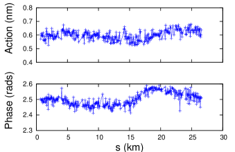
Figure 1: Action and phase plots of an average trajectory obtained from an experimental TBT data set collected at the 2016 LHC run.

These variations are a combination of slow and fast oscillations that can be understood by simulations with different sources of errors. The slow oscillations can be attributed to quadrupole tilt errors, as can be seen from the red curve of Fig. 2. This curve corresponds to the action plot of a simulated average trajectory generated with a quadrupole tilt error distribution with 2 mrad standard deviation.

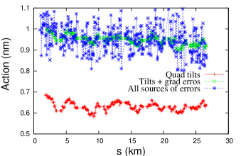
Figure 2: Action plots of simulated average trajectories with coupling and other sources of errors.

The fast oscillations can be attributed to BPM gain and noise errors and uncertainties related to the determination of the lattice functions. This is confirmed by the action plot (blue curve of Fig. 2) of a simulated TBT data set generated with error distributions with the currently accepted rms values for the LHC: 3% rms BPM gain errors Valdivieso and Tomás (2020), 0.1 mm rms BPM noise Malina (2019), 1% rms uncertainties in the determination of the beta functions Langner and Tomás (2015); Wegscheider et al. (2017), 6 mrads rms uncertainties in the determination of the betatron phases Skowroński et al. (2016), 2 mrad rms quadrupole tilt errors, and $5*10^{-6}$ $m^{-2}$ rms gradient errors. It should be noted that the amplitude of the slow oscillations can be comparable to the amplitude of the fast oscillations, indicating that the quadrupole tilt errors may be as important as the other sources of errors in accurately finding $J_{c}$ and $\delta_{c}$. It should also be noted that the amplitude of the fast oscillations in the simulations is larger than in the experimental data. This may indicate that one or all of the sources of these oscillations are smaller than the currently accepted values. In Sec. V, in fact, it is found that the rms values of the calibration factors are somewhat smaller than the 3% mentioned earlier.

Gradient errors alone shift the action and phase plots vertically, changing the $J_{c}$ and $\delta_{c}$ values that can be estimated from these plots. These changes, however, do not affect the estimate of $z_{true}$ as long as the lattice functions that include the gradient errors are used in Eq. (2). The displacement of the action plot can be seen by comparing the red and the green curves in Fig. 2. The green curve is an action plot obtained with the 2 mrad rms quadrupole tilt error distribution used in the red curve plus a $5*10^{-6}$ $m^{-2}$ rms gradient error distribution.

IV Building average trajectories to reduce the effect of coupling

Average trajectories are built by selecting trajectories from a TBT data set according to (complete procedure in Sec. V of Cardona et al. (2017))

$$\left|\tilde{\delta}_{z}(n_{m})-\tilde{\delta}_{z}(n)\right|<\frac{\pi}{2},$$ (5)

where $\tilde{\delta}_{z}(n)$ is the phase (as defined in Cardona et al. (2017)) associated with the trajectory with turn number $n$, and

$$\tilde{\delta}_{z}(n_{m})=\psi_{z}(s_{e})-p\frac{\pi}{2},$$ (6)

where $\psi_{z}(s_{e})$ is the nominal betatron phase at the axial position where the average trajectory should be a maximum, and $p$ is an odd, positive or negative number. Regular average trajectories are built using one-turn trajectories that satisfy the condition (5) in both planes simultaneously. As a consequence, about a thousand of one-turn trajectories are selected from the 6600 turns contained on a TBT data set. Now, if this condition is imposed to only one plane, the number of selected trajectories increases to half the total number of trajectories in the TBT data set. More importantly, the average trajectory in the plane for which the condition is not imposed tends to be negligible. If this procedure is applied to an experimental TBT data set (the same one used to obtain Fig. 1), the corresponding average trajectory has significantly smaller oscillations in one plane than in the other, as expected (Fig. 3).

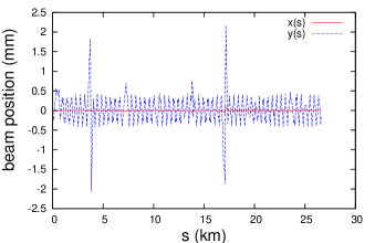
Figure 3: Average trajectory obtained by selecting one-turn trajectories from experimental TBT data that satisfy the condition (5) only in the vertical plane. As a consequence, the oscillations in the vertical plane are significantly larger than in the horizontal plane. It is also possible to built average trajectories with large oscillations in the horizontal plane and significantly smaller in the vertical plane.

Significantly reducing the amplitude of the oscillations in one of the planes also reduces the effect of linear coupling in the other plane, as can be seen in the action and phase plots in Fig.  4.

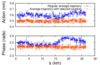
Figure 4: Action and phase plots obtained with average trajectories built by applying condition 5 to both planes and to a single plane. The slow oscillations, corresponding to quadrupole tilt errors, are significantly decreased with the new average trajectories.

In addition to the average trajectory with a maximum at $s_{e}$ (max trajectory), it is also possible to built an average trajectory with a minimum at $s_{e}$ (min trajectory). These two trajectories can be subtracted to obtain a max trajectory that now is built from all the 6600 turns in the TBT data set.

V Measuring Gain Errors in Arc BPMs

All improvements mentioned in previous sections are used to find arc BPM calibration factors with Eqs. (1) and (2), where all relevant variables are found from average trajectories derived from TBT data and lattice functions. Both, simulations and experimental analysis are presented in the following subsections where two conventions are adopted: first, the “measured” calibration factors correspond to the factors obtained with Eqs. (1) and (2) regardless of whether simulated or experimental data is used, and second, the gain errors $\varepsilon_{g,i}$ and the calibration factors $C_{i}$ are related by

$$\varepsilon_{g,i}=C_{i}-1$$ (7)

V.1 Arc BPM calibration factors from simulations

To evaluate the accuracy (as defined in of the Joint Committee for Guides in Metrology (2008)) of this part of the calibration method, simulated TBT data with the errors listed in Table 1 are generated with MADX Grote et al. (2015). The new lattice functions (nominal lattice plus gradient errors) are also generated by MADX and, in addition, the uncertainties associated with the determination of the lattice functions listed in Table 1 are added. TBT data and lattice functions are then used to obtain the action and phase plots and the measured BPM gain errors.

Table 1: Rms values of known errors in the LHC lattice (first three rows) and uncertainties associated with the determination of lattice functions (last two rows).

Errors	Rms value	Extracted from:
Gradients	$5*10^{-6}$ $m^{-2}$	Fol et al. (2019)
BPM gains	3%	Valdivieso and Tomás (2020)
Arc BPMs noise	0.1 mm	Malina (2019)
$\qquad\beta_{r}(s)$	1%	Langner and Tomás (2015); Wegscheider et al. (2017)
$\qquad\psi_{r}(s)$	6 mrads	Skowroński et al. (2016)

An histogram of all the measured arc BPM gain errors obtained in this simulation for the vertical plane of beam 2 can be seen in Fig. 5 (red bars). The same figure also shows the histogram of the differences between the measured BPM gain errors and their corresponding true values (green bars). These histograms illustrate that calibration factors with an original 3% rms distribution can be reduced to a 0.8% rms calibration factors distribution.

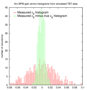
Figure 5: The red histogram corresponds to the measured gain errors of the arc BPMs obtained from a simulated TBT data set. The standard deviation of the distribution is around 3% as expected. The green histogram is the difference between the measured BPM gain errors and the true gain errors used in the simulation. The standard deviation of this histogram indicates that the accuracy of the calibration for the arc BPMs is approximately 0.8% rms.

If the measured gain errors are used to calibrate the original simulated TBT data set, clear reductions in the variations of their corresponding action and phase plots can be seen ( Fig. 6 ).

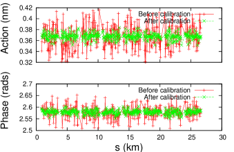
Figure 6: The action and phase plots of the simulated average trajectory with errors in Table 1 show a significant reduction of oscillations after calibration.

V.2 Arc BPM calibration factors from experimental data

A few TBT data sets taken during the 2016 LHC run are used to find the calibration factors of the arc BPMs. These TBT data sets were taken after global and local coupling corrections were applied on the IRs, but there were no quadrupole corrections for gradient errors in the IRs. The lattice functions are obtained directly from the same TBT data sets using the most up-to-date algorithms, currently used in the LHC and automatically provided by the orbit and measurement correction (OMC) software Carlier et al. (2019). Once the experimental TBT data and lattice functions are available, same procedure used to obtain calibration factors from simulated data is also used with 5 TBT data set of beam 1 and 5 TBT data sets of beam 2. As an example, the gain error histogram for the BPMs in the vertical plane of beam 2 is shown in Fig. 7.

Figure 7: Histogram of arc BPM gain errors (vertical plane) measured from an experimental TBT data of beam 2. Calibration factors in this histogram are distributed within a standard deviation of 2.2% rms (2.3% rms in the horizontal plane).

This histogram indicates that the rms gain error in the arc BPMs is around 2%, which is slightly smaller than the 3% reported in Valdivieso and Tomás (2020). Using the measured gain errors, the experimental TBT data set is calibrated, leading to cleaner action and phase plots, as seen in Fig 8.

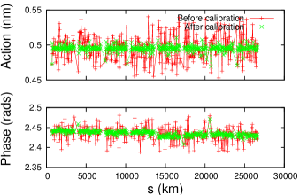
Figure 8: Action and phase plots of an experimental TBT data set before and after the calibration factors in Fig. 7 are applied.

VI Measuring Gain Errors in IR BPMs

In each quadrupole triplet of the low $\beta^{*}$ IRs there are 3 BPMs: BPMSW, BPMS and BPMYS. To find their calibration factors two different methods are used.

VI.1 Method to find calibration factors of BPMSWs

The calibration method for these BPMs is essentially the same as for the BPM arcs. The difference is that the beta functions are estimated from k-modulation experiments Carlier and Tomás (2017). These experiments provide the minimum value of the beta function between the triplets $\beta_{w}$ (commonly known as the beta function at the waist), and the distance between the position of the waist and the center of the inter-triplet space $w$ (commonly known as the waist shift). The beta functions at the BPMSWs are

$$\beta(s^{\pm}_{b})=\beta_{w}+\frac{(L\pm w)^{2}}{\beta_{w}}$$ (8)

where $s^{\pm}_{b}$ are the axial position of the BPMSWs located in the left and right triplets and $L$ is half the length of the inter-triplet space. The equation (8) leads to very accurate measurement of the $\beta$ functions at the two BPMSWs, which should also allow a more accurate BPM calibration.

VI.2 Method to find calibration factors of BPMS and BPMYS

For BPMS and BPMYS, the k-modulation technique is currently not available, but a modification of the method for finding the calibration factors can take advantage of the accurate calibration of the BPMSWs.

Suppose that a particle of beam 1, coming from the inter-triplet space of IR1, passes through BPMSW registering a beam position $z(s_{b})$. The particle then passes through the first quadrupole of the right triplet (Q1) and then arrives to BPMS, where a beam position $z(s_{s})$ is recorded. According to the action and phase method, any one-turn particle trajectory can be described by

$$z(s)=\sqrt{J(s)\beta_{n}(s)}\sin\left[\psi_{n}(s)-\delta(s)\right],$$ (9)

where the subscripts $n$ are used to refer to the nominal variables. Hence,

$$z(s_{b}) = \sqrt{J(s_{b})\beta_{n}(s_{b})}\sin\left[\psi_{n}(s_{b})-\delta(s_{b})\right]$$ (10)

$$z(s_{s}) = \sqrt{J(s_{s})\beta_{n}(s_{s})}\sin\left[\psi_{n}(s_{s})-\delta(s_{s})\right].$$ (11)

On the other hand, $z(s_{s})$ can also be expressed based on the original action and phase $J(s_{b})$ and $\delta(s_{b})$ plus the kick $\theta$ experienced by the particle due to a magnetic error present in Q1 at $s_{e}$ (see Eq. (1) of reference Cardona et al. (2017))

$$z(s_{s}) = \sqrt{J(s_{b})\beta_{n}(s_{s})}\sin\left[\psi_{n}(s_{s})-\delta(s_{b})\right]+$$

$$\theta\sqrt{\beta_{n}(s_{s})\beta_{n}(s_{e})}\sin\left[\psi_{n}(s_{s})-\psi_{n}(s_{e})\right],$$

The phase advance between $s_{s}$ and $s_{e}$ is negligible and hence

$$z(s_{s})=\sqrt{J(s_{b})\beta_{n}(s_{s})}\sin\left[\psi_{n}(s_{s})-\delta(s_{b})\right].$$ (13)

Finally, using Eqs. (10) and (13)

$$z(s_{s})=z(s_{b})\sqrt{\frac{\beta_{n}(s_{s})}{\beta_{n}(s_{b})}}\frac{\sin\left[\psi_{n}(s_{s})-\delta(s_{b})\right]}{\sin\left[\psi_{n}(s_{b})-\delta(s_{b})\right]},$$ (14)

which allows estimating $z(s_{s})$ from the nominal lattice functions and $z(s_{b})$ that is already calibrated. $\delta(s_{b})$ corresponds to the phase in the inter-triplet space $\delta_{t}$ and can be estimated with the formulas developed and tested in Cardona et al. (2020). A similar procedure can be used to estimate the beam position at BPMSY.

VI.3 IR BPM calibration factors from simulations

Two hundred simulated TBT data sets with the errors listed in Table 2 are generated with MADX to asses the accuracy of the calibration methods presented in this section.

Table 2: In addition to the errors and uncertainties listed in Table 1, the uncertainties associated to k-modulation experiments are included since the beta functions derived from these experiments are used for calibration of IR BPMs.

Errors	Rms value	Extracted from:
Grads	$5*10^{-6}$ $m^{-2}$	Fol et al. (2019)
BPM gains	3%	Valdivieso and Tomás (2020)
Arc BPMs noise	0.1 mm	Malina (2019)
$\qquad\beta_{r}(s)$	1%	Langner and Tomás (2015); Wegscheider et al. (2017)
$\qquad\psi_{r}(s)$	6 mrads	Skowroński et al. (2016)
Trip. quad grads	$2*10^{-5}$ $m^{-2}$	Persson et al. (2017)
Match quad grads	$1*10^{-4}$ $m^{-2}$	Cardona et al. (2020)
$\qquad w_{r}$	1 cm	k-modulation experiments
$\qquad\beta_{w_{r}}$	0.3 mm	k-modulation experiments

Random calibration factors with a standard deviation of 3% rms are assigned to the triplet BPMs plus a systematic shift of 5% with respect to the calibration factors of the arcs (as suggested by Valdivieso and Tomás (2020)). Since there are two hundred simulations, there are two hundred measured calibration factors obtained with Eq. (14) and two hundred true calibration factors for every IR BPM. The rms differences of these two quantities are reported in Table 3 for the six beam-2 BPMs in IR1. Also, Fig. 9 shows a histogram of the measured gain error minus the true gain errors for BPMSW.1L1. Similar histograms can be found for the other 5 BPMs.

Table 3: Rms differences between measured calibration factors and true calibration factors for 200 simulations. The errors listed in Table 2 are added to each simulation according to a Gaussian distribution with the indicated standard deviations.

	Rms accuracy
BPM	(%)
BPMSW.1L1.B2	0.34
BPMSW.1R1.B2	0.3
BPMSY.4L1.B2	0.42
BPMS.2L1.B2	0.23
BPMS.2R1.B2	0.28
BPMSY.4R1.B2	0.28

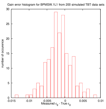
Figure 9: Histogram of the differences between the measured gain errors and the true gain errors in BPMSW.1L1 for 200 hundred simulations with the random errors in Table 2 . The standard deviation of this histogram indicates that the calibration accuracy for BPMSW.1L1 is approximately 0.3% rms with the method presented in this section.

VI.4 IR BPM calibration factors from experimental data

The same 5 experimental TBT data sets of beam 1 and the 5 TBT data sets of beam 2 mentioned in Sec. V are used to find the calibration factors for the IR BPMs. Furthermore, data from k-modulation experiments performed simultaneously while taking the experimental TBT data are used to estimate the beta functions in the BPMSWs with Eq. (8). These analyses finally lead to calibration factors for the 6 triplet BPMs of beam 1 and the six triplet BPMs of beam 2 in both planes, as can be seen in Table 4 5.

Table 4: Calibration Factor for IR1 BPMs obtained from 2016 experimental TBT and k-modulation data of beam 1.

	Beam 1 Calibration Factors
BPM Name	HOR	VERT
BPMSW.1L1	$0.968\pm 0.001$	$0.942\pm 0.001$
BPMSW.1R1	$0.961\pm 0.001$	$0.906\pm 0.001$
BPMS.2L1	$0.954\pm 0.001$	$0.926\pm 0.001$
BPMS.2R1	$0.981\pm 0.001$	$0.941\pm 0.002$
BPMSY.4R1	$0.928\pm 0.001$	$0.939\pm 0.001$

Table 5: Calibration Factor for IR1 BPMs obtained from 2016 experimental TBT and k-modulation data of beam 2.

	Beam 2 Calibration Factors
BPM Name	HOR	VERT
BPMSW.1L1	$0.953\pm 0.002$	$0.942\pm 0.001$
BPMSW.1R1	$0.935\pm 0.001$	$0.944\pm 0.001$
BPMSY.4L1	$0.951\pm 0.001$	$0.948\pm 0.002$
BPMS.2L1	$0.942\pm 0.001$	$0.941\pm 0.001$
BPMS.2R1	$0.947\pm 0.002$	$0.954\pm 0.002$
BPMSY.4R1	$0.955\pm 0.001$	$0.979\pm 0.001$

IR BPM Calibration factor are shifted about 5% as reported in Valdivieso and Tomás (2020). The experimental uncertainty is estimated as the standard deviation of the five measurements available for every calibration factor and it is remarkably small.

VII BPM gain errors and quadrupole corrections in the IRs

Corrections to linear magnetic errors in the IRs can be estimated with the action and phase jumps that can be seen in action and phase plots obtained with nominal lattice functions Cardona et al. (2017, 2020). Since these plots are derived from BPM measurements, it is necessary to asses their sensitivity to BPM calibrations. To evaluate this sensitivity, the calibration factors found for the arc and IR BPMs in Secs. V and VI are applied to the same experimental TBT data sets used in those sections and the corresponding action and phase plots are obtained (Fig. 10). Comparisons between the action and phase plots before and after calibration show significant improvements, particularly in the action plots.

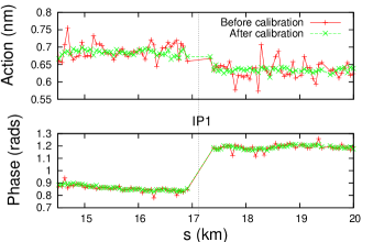
Figure 10: Action and Phase jump in the horizontal plane of beam 2 at IR1 before and after applying the BPM calibration. The calibration procedure make it possible to define the jump more clearly, especially in the action plot.

Also, since now the average trajectories are much larger in one plane than the other, the simplified expressions

$${B_{1}}_{x,e} = -\frac{\theta_{x,e}}{x_{e}},$$ (15)

$${B_{1}}_{y,e} = \frac{\theta_{y,e}}{y_{e}}$$ (16)

can be used to estimate the quadrupole components ${B_{1}}_{z,e}$ of the equivalent kick $\theta_{x,e}$ instead of Eqs. (7) of Cardona et al. (2020). Once these components are known, the corrections are estimated before and after calibration and no significant variations are found (Table 6). The equivalence between the two corrections can also be verified through the beta-beating that they produce as can seen in Fig. 11.

Table 6: Quadrupole correction estimated for IR1 from experimental TBT data before and after the calibration procedure. Most of the proposed corrections in the 12 quadrupoles have only small variations between the two cases.

	Correction strengths
	($10^{-5}$ $m^{-2}$)
Magnet	Before calibration	After calibration
Q2L	$1.24$	$1.19$
Q2R	$-0.84$	$-0.76$
Q3L	$1.44$	$1.36$
Q3R	$-2.75$	$-2.60$
Q4L.B1	$11.3$	$10.2$
Q4L.B2	$-11.3$	$10.2$
Q4R.B1	$-8.0$	$-8.2$
Q4R.B2	$8.0$	$8.2$
Q6L.B1	$-41.1$	$-35.9$
Q6L.B2	$34.2$	$29.9$
Q6R.B1	$25.4$	$27.4$
Q6R.B2	$-22.2$	$-24.0$

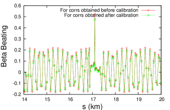
Figure 11: Beta-beating generated by the corrections obtained before and after BPM calibration. Based on the small differences in the two plots, it can be stated that the two corrections are equivalent.

VIII Other Simulations

The results of Sec. V indicate that arc BPM gain errors are approximately 2.3% rms. Also, the current number of turns has been increased to 10000, which reduces the effect of electronic noise. Except fo these changes, TBT data sets are simulated with the same errors listed in Table 1. The calibrations factors of the BPM arcs can now be recovered with 0.7% accuracy instead of the original 0.8% quoted in Sec. V. The IR BPMs calibrations also have a better associated accuracy, as can be seen comparing Tables 7 and 3.

Table 7: Rms differences between measured calibration factors and true calibration factors for 200 simulations. Table 2 is still used in the simulations, except that gain errors are now 2.3% and the electronic noise corresponds to what would exist for 10000 turns.

	Rms accuracy
BPM	(%)
BPMSW.1L1.B2	0.26
BPMSW.1R1.B2	0.25
BPMSY.4L1.B2	0.38
BPMS.2L1.B2	0.19
BPMS.2R1.B2	0.26
BPMSY.4R1.B2	0.26

IX Conclusions

A method has been developed to find calibrations factors based on average trajectories. Simulations show that the calibration factors for arc BPMs can be recovered with an accuracy of 0.7% rms and the calibatrion factors for IR BPMs can be recovered with an accuracy of 0.4% rms. The method has been used to obtain the calibration factors of six BPMs of beam 1 and six BPMs of beam 2 at the IR1 of the LHC. For these estimates, several TBT data sets, measured lattice functions, and k-modulation measurements in the IRs are needed.

This method has also been used to test the BPM calibration sensitivity of the action and phase jump method. Although the calibration helps to more clearly define the action and phase jump in the IR, its effect on the estimation of corrections is negligible.

References

- Cardona et al. (2017) J. F. Cardona, A. C. García Bonilla, and R. Tomás García, Phys. Rev. Accel. Beams 20, 111004 (2017).
- Carlier et al. (2019) F. Carlier, J. Coello, J. Dilly, E. Fol, A. Garcia-Tabares, M. Giovannozzi, M. Hofer, E. H. Maclean, L. Malina, T. Persson, P. Skowronski, M. Spitznagel, R. Tomás, A. Wegscheider, J. Wenninger, J. Cardona, and Y. Rodriguez, in Proceedings of the 2019 International Particle Accelerator Conference (2019) p. 2773.
- Cardona et al. (2020) J. F. Cardona, Y. Rodríguez, and R. Tomás, “A twelve-quadrupole correction for the interaction regions of high-energy accelerators,” (2020), arXiv:2002.05836 [physics.acc-ph] .
- Valdivieso and Tomás (2020) A. G.-T. Valdivieso and R. Tomás, Phys. Rev. Accel. Beams 23, 042801 (2020).
- Malina (2019) L. Malina, “Lhc bpm performance: noise,” OMC-BI meeting (2019).
- Langner and Tomás (2015) A. Langner and R. Tomás, Phys. Rev. ST Accel. Beams 18, 031002 (2015).
- Wegscheider et al. (2017) A. Wegscheider, A. Langner, R. Tomás, and A. Franchi, Phys. Rev. Accel. Beams 20, 111002 (2017).
- Skowroński et al. (2016) P. Skowroński, F. Carlier, J. C. de Portugal, A. Garcia-Tabares, A. Langner, E. Maclean, L. Malina, M. McAteer, T. Persson, B. Salvant, and R. Tomás, in Proceedings of IPAC 2016 (2016).
- of the Joint Committee for Guides in Metrology (2008) W. G. . of the Joint Committee for Guides in Metrology, Evaluation of measurement data — Guide to the expression of uncertainty in measurement, BIPM, IEC, IFCC, ILAC, ISO, IUPAC, IUPAP and OIML (2008).
- Note (1) Closeness of the agreement between the result of a measurement and a true value of the measurand.
- Grote et al. (2015) H. Grote, F. Schmidt, L. Deniau, and G. Roy, The MAD-X Program, European Organization for Nuclear Research (2015).
- Fol et al. (2019) E. Fol, J. C. de Portugal, G. Franchetti, and R. Tomás, in Proceedings of IPAC 2019 (2019) p. 3990.
- Carlier and Tomás (2017) F. Carlier and R. Tomás, Phys. Rev. Accel. Beams 20, 011005 (2017).
- Persson et al. (2017) T. Persson, F. Carlier, J. Coello de Portugal, A. Garcia-Tabares Valdiveso, A. Langner, E. H. Maclean, L. Malina, P. Skowronski, B. Salvant, R. Tomás, and A. C. García Bonilla, PRAB 20, 061002 (2017).