Flat and Correlated Plasmon Bands in Graphene/$\alpha$-RuCl₃ Heterostructures

Abstract

We develop a microscopic theory for plasmon excitations of graphene/$\alpha$-RuCl₃ heterostructures. Within a Kondo-Kitaev model with various interactions, a heavy Fermi liquid hosting flat bands emerges in which the itinerant electrons of graphene effectively hybridize with the fractionalized fermions of the Kitaev quantum spin liquid. We find novel correlated plasmon bands induced by the interplay of flat bands and interactions and argue that our theory is consistent with the available experimental data on graphene/$\alpha$-RuCl₃ heterostructures. We predict novel plasmon branches beyond the long-wavelength limit and discuss the implications for probing correlation phenomena in other flat band systems.

Introduction.— Plasmons are collective charge oscillations whose properties are normally dominated by the long-range Coulomb interactions in low density systems Pines and Bohm (1952); Pines (1956). However, strong correlations can drastically alter their behavior which allows to probe new quantum many-body physics with optical experiments. For example, Kondo interactions can give rise to new low energy plasmon modes in heavy fermion materials Millis et al. (1987); Millis and Coppersmith (1990); Freytag and Keller (1990) or can distort the surface collective modes in topological Kondo insulators Efimkin and Galitski (2014). A local Hubbard interaction also leads to a strong renormalization of the plasmon dispersion and a shift of spectral weight van Loon et al. (2014); Greco et al. (2016); Yin et al. (2019). Apart from strong interactions, it is of course the form of the electronic bandstructure which determines the properties of plasmons. For example, monolayer graphene serves as an outstanding platform for the study of Dirac plasmons Wunsch et al. (2006); Hwang and Das Sarma (2007); Bonaccorso et al. (2010); Avouris (2010); Ju et al. (2011); Koppens et al. (2011); Grigorenko et al. (2012); Chen et al. (2012); Stauber (2014) with a low-energy and long-wavelength dispersion, $\omega\propto{}\sqrt{q}$, and the van Hove singularity of the dispersion leads to so-called $\pi$ plasmons which have been observed in monolayer graphene with electron energy loss spectroscopy Eberlein et al. (2008); Kinyanjui et al. (2012); Stauber et al. (2010).

The advent of two-dimensional (2D) heterostructures has paved the way for investigating new correlation and bandstructure effects on plasmon modes. For instance, twisted bilayer graphene (TBG), the moiré material which hosts strongly correlated flat bands Cao et al. (2018a, b), shows novel collective plasmon excitations Stauber and Kohler (2016); Lewandowski and Levitov (2019); Khaliji et al. (2020); Novelli et al. (2020); Hesp et al. (2019); Hu et al. (2017); Fahimniya et al. (2020). Apart from the conventional 2D Dirac plasmons which are damped as momentum $q$ increases and merge with the particle-hole (p-e) continuum Wunsch et al. (2006); Hwang and Das Sarma (2007), it is reported that the plasmons in TBG and other narrow-band materials exhibit flat and weakly damped dispersions piercing through the p-e continuum Lewandowski and Levitov (2019); Khaliji et al. (2020); Novelli et al. (2020).

Recently a new graphene/$\alpha-$RuCl₃ heterostructure has attracted significant attention Zhou et al. (2019); Mashhadi et al. (2019); Wang et al. (2020); Rizzo et al. (2020), since the Mott insulating $\alpha-$RuCl₃ layer is a promising candidate for realizing the seminal Kitaev quantum spin liquid (QSL) Kitaev (2006); Rau et al. (2016); Winter et al. (2017); Hermanns et al. (2018); Takagi et al. (2019). The quasi-2D material $\alpha-$RuCl₃ has long-ranged magnetism at low temperatures due to additional interactions beyond the bond oriented Kitaev exchange but is believed to be in proximity to a QSL phase Banerjee et al. (2016). The lattice-mismatch between graphene and $\alpha-$RuCl₃ induces strain which has been shown to enhance the Kitaev spin exchange Biswas et al. (2019); Gerber et al. (2020) bringing the system closer to the Kitaev QSL with its fractionalized Majorana fermion excitations. However, the graphene layer is also strongly affected because of a charge transfer from the itinerant to the insulating layer as observed experimentally Mashhadi et al. (2019); Wang et al. (2020); Rizzo et al. (2020) and in accordance with ab-initio calculations Biswas et al. (2019). Graphene becomes hole-doped and $\alpha-$RuCl₃ electron-doped with the Fermi energy lying within the correlated narrow Ru-band which is almost flat in the Brillouin zone except for a small hybridization region Biswas et al. (2019). Recent experiments have observed plasmons in graphene/$\alpha-$RuCl₃ heterostructures with an excess damping mechanism attributed to the correlated insulating layer Rizzo et al. (2020). However, it is an outstanding question how the unusual excitations are linked to correlation effects of $\alpha-$RuCl₃? More generally, it has remained unexplored whether plasmonic excitations can be used to probe correlation effects related to QSL fluctuations in correlated heterostructures?

In this work, we show that the interplay of correlated flat bands and strong local interactions can lead to novel plasmon excitations. We develop a microscopic theory of collective charge excitations in a minimal bilayer Kondo-Kitaev lattice model of $\alpha-$RuCl₃ on top of graphene with interlayer spin-only Kondo couplings. The Kondo-Kitaev model has a rich phase diagram displaying a fractionalized Fermi liquid, $p$-wave superconductivity, and heavy Fermi-liquid (hFL) phase as calculated within a self-consistent Abrikosov fermion mean-field theory Choi et al. (2018); Seifert et al. (2018). In the hFL phase, the fractionalized fermions of the Kitaev QSL acquire charge by hybridizing with the itinerant electrons from graphene which results in an almost flat Dirac band at the Fermi energy whose bandwidth is set by the Kitaev exchange and a hybridization by the local Kondo coupling, see Fig.1 (a). Recently, it was shown that ab-initio calculations and experimental constraints can be used to determine the microscopic parameters of the effective low energy hFL band structure, which has been employed to explain the non-Lifshitz Kosevich temperature dependence of quantum oscillations measured in graphene/$\alpha$-RuCl₃ heterostructures Leeb et al. (2021).

Here, we calculate the dynamical charge susceptibility for the hFL phase and study the plasmon dispersions over the Brillouin zone in both low- and high-energy scales taking into account the effect of different local interactions. As the main result, we find new plasmonic modes whose small momentum behavior is consistent with recent experiments on graphene/$\alpha$-RuCl₃ heterostructure Rizzo et al. (2020).

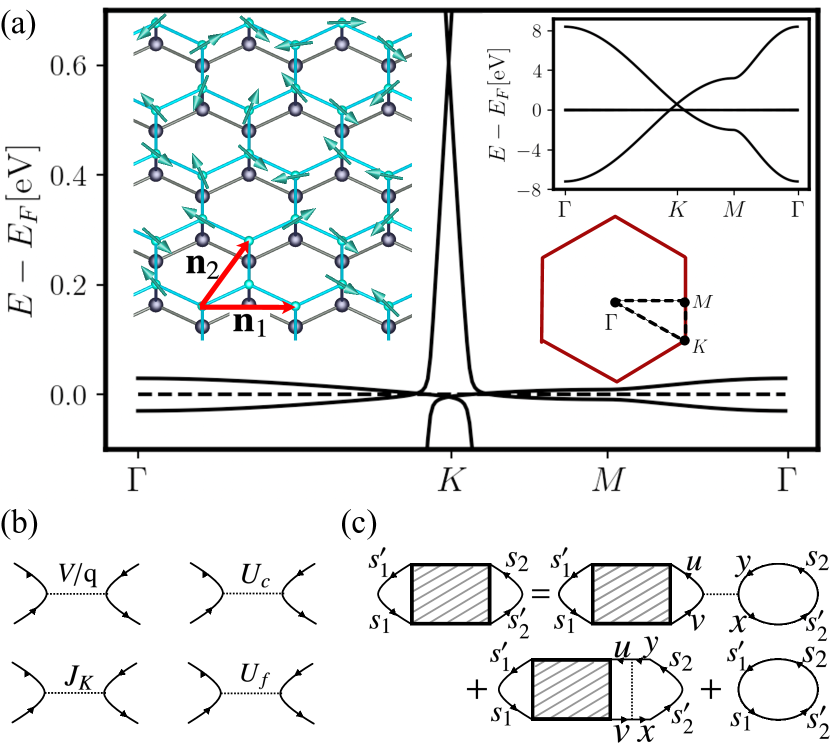
Figure 1: (a) The band structures of the effective model Eq. (13) with $u=0.6$ eV, $t=2.6$ eV, $J=0.1$ eV, and $K=0.01$ eV Leeb et al. (2021). The dashed line is the Fermi energy $E_{F}=0$. The left inset plot shows the schematic picture of the Kitaev-graphene lattice and corresponding lattice vectors $\bm{n}_{1}$ and $\bm{n}_{2}$. The upper layer with $S=1/2$ spins depicts for Kitaev Mott insulator and the other one the itinerant graphene layer. The right inset plots shows the whole band structure and the Brillouin zone of honeycomb lattice. (b) Diagrammatic representations of the Coulomb interaction $V/{q}$, on-site Hubbard repulsion $U_{c}(f)$ and $U_{f}$, and Kondo couplings $J_{K}$. (c) The diagrammatic representation of the Dyson equation for the RPA charge susceptibility.

Effective model of a Kitaev-Graphene system.— Our starting point is the Kondo-Kitaev lattice model with a ferromagnetic Kitaev layer in which the $S=1/2$ spins $\bm{S}_{i}$ are coupled to conduction electrons via the on-site antiferromagnetic Heisenberg Kondo coupling. Within the framework of a parton theory, the $S=1/2$ spins can be represented as bilinear forms of Abrikosov fermions, $\bm{S}_{i}=\frac{1}{2}f^{\dagger}_{i\sigma}\bm{\tau}_{\sigma\sigma^{\prime}}f_{i,\sigma^{\prime}}$, where $\bm{\tau}=(\tau^{x},\tau^{y},\tau^{z})$ are three Pauli matrix and the summation over repeated spin indices $\sigma$’s is assumed. This representation enlarges the Hilbert space and a local constraint $\sum_{\sigma}f^{\dagger}_{i\sigma}f_{i\sigma}=1$ has to be imposed to restore the physical Hilbert space of spin-1/2’s. Within a self-consistent parton mean-field solution, a hFL phase is realized in a large part of the phase diagram Choi et al. (2018); Seifert et al. (2018) described by a quadratic Hamiltonian $H_{0}$, which has recently been shown to capture the essential aspects of the graphene/$\alpha-$RuCl₃ electronic structure Leeb et al. (2021). In momentum space, it is expressed in terms of itinerant electrons $c_{s,\bm{k},\sigma}$ and Abrikosov fermions $f_{s,\bm{k},\sigma}$ ($s=1,2$) as Seifert et al. (2018); Leeb et al. (2021)

$$H_{0}=\sum_{\sigma,\bm{k}}\left(\begin{array}[]{l}c_{1,\bm{k},\sigma}\\ c_{2,\bm{k},\sigma}\\ f_{1,\bm{k},\sigma}\\ f_{2,\bm{k},\sigma}\end{array}\right)^{\dagger}\left(\begin{array}[]{cccc}W&t\theta^{*}_{\bm{k}}&J/2&0\\ t\theta_{\bm{k}}&W&0&J/2\\ J/2&0&0&K\theta^{*}_{\bm{k}}\\ 0&J/2&K\theta_{\bm{k}}&0\\ \end{array}\right)\left(\begin{array}[]{l}c_{1,\bm{k},\sigma}\\ c_{2,\bm{k},\sigma}\\ f_{1,\bm{k},\sigma}\\ f_{2,\bm{k},\sigma}\end{array}\right),$$ (13)

where $\theta_{\bm{k}}=1+\exp(i\bm{k}\cdot\bm{n}_{1})+\exp(i\bm{k}\cdot\bm{n}_{2})$, $t$ ($K$) is the band parameter of $c$- ($f$-) fermions , $J$ is the hybridization strength, and $W$ is the energy shift between the graphene Dirac cone of $c$-fermions and the Kitaev Dirac cone of $f$-fermions. Note that the low energy scales $K,J$ are set by the Kitaev and Kondo exchange. Throughout this work, we consider the regime $t\gg{}K$ and $t>J$, where the Kitaev Dirac bands are almost flat. For convenience, we also adapt the notation of $c_{3(4),\bm{k},\sigma}\equiv{}f_{1(2),\bm{k},\sigma}.$ The characteristic energy spectrum of $H_{0}$ is shown in Fig. 1 (a). The hopping parameter is fixed as $t=2.6$ eV to adapt the slope of the graphene Dirac cone and the large energy shift $W\approx 0.6$ eV is in accordance with the charge transfer from graphene to $\alpha$-RuCl₃ Biswas et al. (2019). The Fermi energy ($E_{F}=0$) lies with the two flat Kitaev Dirac bands.

We are interested in the interaction induced fluctuations on top of this effective electronic structure and, therefore, concentrate on the following Hamiltonian

$$H_{\text{hetero}}=H_{0}+H^{(f)}_{\text{U}}+H^{(c)}_{\text{U}}+H_{\text{C}}+H_{\text{K}},$$ (14)

where the last four terms are quartic interaction terms. As mentioned above, the Abrikosov fermions have a local singly-occupancy constraint which can be effectively imposed by an on-site Hubbard term $H^{(f)}_{\text{U}}=U_{f}/2\sum_{s,\bm{r},\sigma}\left(f^{\dagger}_{s,\bm{r},\sigma}f_{s,\bm{r},{\sigma}}f^{\dagger}_{s,\bm{r},-\sigma}f_{s,\bm{r},-\sigma}\right)$, where the convention that $\sigma=1~{}(-1)$ for spin $\uparrow$ ($\downarrow$) has been adapted. In practice, we will keep the on-site Hubbard $U_{f}$ very large but finite to enforce the constraint of $f-$fermions. $H^{(c)}_{\text{U}}$ is an additional Hubbard term for $c$-fermions parameterized by repulsive strength $U_{c}$. The fourth term, $H_{\text{C}}$, is the Coulomb interaction and reads $H_{\text{C}}=\frac{1}{\mathcal{N}}\sum_{s,s^{\prime}=1}^{4}\sum_{\bm{k,k^{\prime},p},\sigma,\sigma^{\prime}}\frac{V}{{q}}e^{-\bm{q}\cdot{}\bm{r}_{ss^{\prime}}}\left(c^{\dagger}_{s,\bm{k+q},\sigma}c_{s,\bm{k},{\sigma}}c^{\dagger}_{s^{\prime},\bm{k^{\prime}-q},{\sigma}^{\prime}}c_{s^{\prime},\bm{k^{\prime}},{\sigma}^{\prime}}\right)$, where $\mathcal{N}$ denotes the number of total sites, $q\equiv|\bm{q}|$, and $\bm{r}_{ss^{\prime}}=0$ [$(\bm{n}_{1}+\bm{n}_{2})/3$] if $s$ and $s^{\prime}$ are on the same (different) sublattice(s). Finally, $H_{\text{K}}$ is the Kondo coupling of strength $J_{K}$ between localized $c$- and $f$-fermions, which reads $H_{\text{K}}=J_{K}/4\sum_{s,\bm{r}}\left(c^{\dagger}_{s,\bm{r},\sigma_{1}}\bm{\tau}_{\sigma_{1}\sigma_{1}^{\prime}}c_{s,\bm{r},\sigma_{1}^{\prime}}\right)\cdot{}\left(f^{\dagger}_{s,\bm{r},\sigma_{2}}\bm{\tau}_{\sigma_{2}\sigma_{2}^{\prime}}f_{s,\bm{r},\sigma_{2}^{\prime}}\right)$. We note that in principle, the hybridization strength $J$ and the Kondo coupling $J_{K}$ only differ by a renormalized mean-field parameter Choi et al. (2018); Seifert et al. (2018); Leeb et al. (2021), but here we treat $J_{K}$ as an independent parameter to investigate its qualitative effect on excitations.

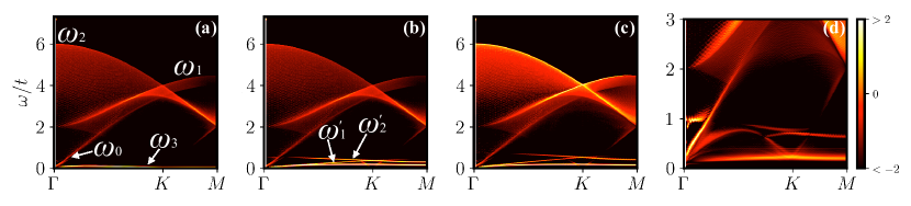
Figure 2: The RPA energy loss function $1/{\rm Im}[\epsilon^{\text{RPA}}(\bm{q},\omega)]$ on a log scale along the $\bm{\Gamma-K-M}$ direction for parameters $J=0.1$ eV, $K=0.01$ eV, $V=6$ eV, and (a) $U_{f}=U_{c}=J_{K}=0$ eV, (b) $U_{f}=120$ eV, $U_{c}=J_{K}=0$ eV, and (c) $U_{f}=240$ eV, $U_{c}=J_{K}=3$ eV. (d) $1/{\rm Im}[\epsilon^{\text{RPA}}(\bm{q},\omega)]$ on a log scale with finite sublattice-symmetry-breaking term of $\sum_{s}(-1)^{s}f^{\dagger}_{s,\bm{k},\sigma}f_{s,\bm{k},\sigma}$ for $J=0.1$ eV, $K=0.01$ eV, $V=3$ eV, $U_{f}=120$ eV, and $U_{c}=J_{K}=3$ eV. For numerical purposes we set the damping constant $\delta\approx{}0.01$ eV app .

Plasmons within a Random Phase Approximation.— As a collective oscillating charge density mode, a plasmon is described by the total response of the systems to external potentials. Thus, it can be characterized by the total dynamical charge correlation function defined as

$$P(\bm{q},\omega)=\sum_{s,s^{\prime}=1}^{4}\sum_{\sigma\sigma^{\prime}}\int_{0}^{\beta}d\tau{}e^{i\omega\tau}\langle{}T_{\tau}\rho_{s\sigma}(\bm{q},\tau)\rho_{s^{\prime}\sigma^{\prime}}(-\bm{q},0)\rangle,$$ (15)

where $\rho_{s\sigma}(\bm{q})=\frac{1}{\mathcal{N}}\sum_{\bm{k}}c^{\dagger}_{s,\bm{k},\sigma}c_{s,\bm{k+q},\sigma}$ is the total density operator ($s=1,...,4$). In order to account for all kinds of interactions in Eq. (14), we define the bare dynamical charge susceptibility tensor as

$$\begin{split}&[\chi^{0}(\bm{q},\omega)]^{s_{1}s_{1}^{\prime}}_{s_{2}s_{2}^{\prime}}=\frac{1}{\mathcal{N}^{2}}\sum_{\bm{k}\bm{k}^{\prime}\sigma\sigma^{\prime}}\int_{0}^{\beta}d\tau{}e^{i\omega\tau}\\ &\langle{}T_{\tau}c^{\dagger}_{s_{1},\bm{k},\sigma}(\tau)c_{s_{1}^{\prime},\bm{k+q},\sigma}(\tau)c^{\dagger}_{s_{2},\bm{k}^{\prime},\sigma^{\prime}}(0)c_{s_{2}^{\prime},\bm{k^{\prime}-q},\sigma^{\prime}}(0)\rangle_{0},\\ \end{split}$$ (16)

where $\langle...\rangle_{0}$ is a canonical ensemble average with respect to the bare Hamiltonian Eq. (13). Up to the zeroth order in interactions, the bare charge correlation function reads $P^{0}(\bm{q},\omega)=\sum_{s,s^{\prime}=1}^{4}[\chi^{0}(\bm{q},\omega)]^{ss}_{s^{\prime}s^{\prime}}$. The interactions then need to be treated self-consistently, leading to the following total dynamical dielectric function $\epsilon(\bm{q},\omega)=P(\bm{q},\omega)/P^{0}(\bm{q},\omega)$ with plasmon excitations given by the zeros of the energy loss function, e.g., the inverse of the imaginary part of $\epsilon(\bm{q},\omega)$.

For analyzing the effect of the different interaction channels we treat the dynamical correlation functions within the random phase approximation (RPA). For graphene, this is well justified for $q\ll{}k_{F}$ with $k_{F}$ the Fermi wavenumber. Plasmon dispersions are determined by the zeros of imaginary part of the RPA dielectric function as $\epsilon^{\text{RPA}}(\bm{q},\omega)=P^{\text{RPA}}(\bm{q},\omega)/P^{\text{0}}(\bm{q},\omega)$ where $P^{\text{RPA}}(\bm{q},\omega)\equiv{}\sum_{ss^{\prime}}[\chi^{\text{RPA}}(\bm{q},\omega)]^{ss}_{s^{\prime}s^{\prime}}$. The RPA charge susceptibility tensor $\chi^{\text{RPA}}(\bm{q},\omega)]^{s_{1}s_{2}}_{s_{1}^{\prime}s_{2}^{\prime}}$ is obtained via a generalized Dyson equation Schrieffer et al. (1989); Chubukov and Frenkel (1992); Knolle et al. (2010) given by

$$\begin{split}&[\chi^{\text{RPA}}]^{s_{1}s_{1}^{\prime}}_{s_{2}s_{2}^{\prime}}=[\chi^{0}]^{s_{1}s_{1}^{\prime}}_{s_{2}s_{2}^{\prime}}+[\chi^{\text{RPA}}]^{s_{1}s_{1}^{\prime}}_{uv}[V^{{l}}-V^{{b}}]^{uv}_{xy}[\chi^{0}]^{xy}_{s_{2}s_{2}^{\prime}},\end{split}$$ (17)

where $V^{b}$ ($V^{l}$) is a vertex for bubble (ladder) diagrams and repeated indices $u,v,x,y$ are summed over. The Dyson equation is schematically shown in Fig. 1 (c). All the tensors in Eq. (17) can be treated as matrices with row index $s_{1}s_{1}^{\prime}$ and column index $s_{2}s_{2}^{\prime}$ and then the solution of Eq. (17) in matrix form is $\chi^{\text{RPA}}=\chi^{0}[1-(V^{{l}}-V^{{b}})\chi^{0}]^{-1}$. The spin indices of the vertices $V^{{b(l)}}$ vanish in Eq.(17) because we have summed over all spin degrees of freedom. The nonzero elements of the bubble contribution are $[V^{{b}}]^{11(33)}_{11(33)}=[V^{{b}}]^{22(44)}_{22(44)}=\frac{4V}{{q}}+U_{c}(U_{f})$, $[V^{{b}}]^{11}_{33}=[V^{{b}}]^{22}_{44}=\frac{4V}{{q}}$, $[V^{{b}}]^{11}_{22(44)}=[V^{{b}}]^{33}_{22(44)}=\frac{4V}{{q}}e^{-\bm{q}\cdot(\bm{n}_{1}+\bm{n}_{2})/3}$ and we have $[V^{{b}}]^{aa}_{cc}=[V^{{b}}]^{cc}_{aa}$. When calculating the ladder diagrams, we ignore the contributions from $\bm{q}$-dependent Coulomb interactions which carry momentum-transfer processes. Consequently, the remaining nonzero elements of the ladder vertex read $[V^{{l}}]^{13}_{31}=[V^{{l}}]^{31}_{13}=[V^{{l}}]^{24}_{42}=[V^{{l}}]^{42}_{24}=J_{K}$. Notice that the contributions from on-site Hubbard repulsion $U_{c}~{}(U_{f})$ for ladder diagrams and from Kondo coupling $J_{K}$ for bubble diagrams are zero after summing over all spin indices.

Numerical results.— For a realistic graphene/$\alpha$-RuCl₃ system, we follow earlier work Leeb et al. (2021) and fix $W=0.6$ eV, $t=2.6$ eV, and $E_{F}=0$ eV to numerically compute $\chi^{(0)}$ and $\chi^{\text{RPA}}$. In general, we are interested in collective excitations over the whole Brillouin zone of the honeycomb model. The results of our calculations are presented in Fig. 2 at zero temperature and for several values of the different interaction parameters.

The graphene subsystem hosts three plasmon bands induced by Coulomb interactions, e.g., one acoustic-like band $\omega_{0}$ as well as two optical bands $\omega_{1}$ and $\omega_{2}$, see Fig. 2 (a). Similar plasmon dispersions in pure graphene systems have been studied beyond the $\bm{k}\cdot\bm{p}$ approximation Stauber et al. (2010); Stauber (2010); Hill et al. (2009). As the graphene Dirac cone at $\mu=0.6$ eV is far away from the Fermi energy, $\omega_{0}$ is dispersing as $\propto{}{q}$ rather than $\propto\sqrt{{q}}$ at lower frequencies and plunges into a p-e continuum at higher frequencies. The two optical bands $\omega_{1}$ and $\omega_{2}$ are degenerate at the $\bm{K}$ point and form a big crossing in the high-symmetry direction $\bm{\Gamma-K-M}$. $\omega_{2}$ hosts co-called $\pi$ plasmons associated with the Van Hove singularity at the $\bm{M}$ point Eberlein et al. (2008); Kinyanjui et al. (2012); Stauber et al. (2010).

In addition to the three graphene plasmon bands, we find a novel low energy plasmon, $\omega_{3}\sim{}J$, see Fig. 2 (a). Note that for illustrative purposes, we have chosen a much larger value of $J\sim{}0.1$ eV than determined in Ref. Leeb et al. (2021). The flat plasmon band originates from the flat electronic bands of the Kitaev layer and barely changes as the interaction couplings vary. However, a finite on-site repulsion $U_{f}$ of the formerly Mott insulating layer leads to two extra plasmon branches above $\omega_{3}$, namely $\omega_{1}^{\prime}$ and $\omega_{2}^{\prime}$, forming a smaller and flatter crossing in the $\bm{\Gamma-K-M}$ direction with an intersection at $\bm{K}$ point, as shown in Fig. 2 (b) and (c). This flatter crossing at low energies only depends on $U_{f}$. It is enlarged and pushed to higher energy region as $U_{f}$ increases, see Fig. 2(c) . Finally, we find that the main effect of moderate Kondo and Hubbard interactions, $J_{K}$ and $U_{c}$, is to enhance the signals of $\omega_{1}$ and $\omega_{3}$ [see Fig. 2 (c)].

We note that there exist a temperature scale above which a crossover from the hFL phase to the decoupled phase occurs Seifert et al. (2018). In the decoupled phase, the hybridization strength renormalizes to zero and consequently the flat plasmon band $\omega_{3}$ and the two emergent bands $\omega^{\prime}_{1}$ and $\omega^{\prime}_{2}$ all disappear. More details about finite temperature effects and disorder broadening can be found in the Supplemental Material app .

An experimentally important aspect so far not accounted for in our minimal model is the lattice mismatch between the two layers, which is expected to gap the flat Dirac cone of the Kitaev layer around $E_{F}$. This can be effectively mimicked by introducing a “$\tau_{z}$” term of $\sum_{s=1,2}(-1)^{s}f^{\dagger}_{s,\bm{k},\sigma}f_{s,\bm{k},\sigma}$ which breaks the sublattice symmetry for the Kitaev layer. We find that a finite and small “$\tau_{z}$” term does not change our main results. However, it pushes the flat plasmon band $\omega_{3}$ to higher energy and opens a small gap at the flat crossing around the $\bm{K}$ point, see Fig. 2 (d). A similar effect on plasmons due to a correlation-driven sublattice asymmetry has been discussed recently in connection with TBG Fahimniya et al. (2020). The sublattice asymmetry endows the plasmons with a dipole moment which is expected to lead to a stronger experimental response.

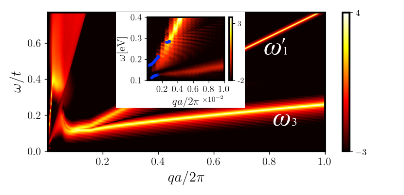
Figure 3: The imaginary part of the inverse RPA dielectric functions $1/{\rm Im}[\epsilon^{\text{RPA}}(\bm{q},\omega)]$ of the linearized Hamiltonian in a log scale with $K=0.05$ eV, $J=0.12$ eV, $V=3$ eV, $U_{c}=J_{K}=1$ eV, and $U_{f}=20$ eV. Inset: Comparison of the plasmon dispersions from experimental data (blue circles) and the linearized low energy model Eq. (14). The model parameters are the same as those in the main plot. The experimental data are collected from Fig. 2 in Ref. Rizzo et al. (2020).

Comparison to experiment.— In experiments, the scattering-scanning near-field optical microscopy (s-SNOM) method Atkin et al. (2012); Basov et al. (2016); Low et al. (2017); Sunku et al. (2018); Ni et al. (2015); Hu et al. (2017) can be used to measure the dispersions of collective charge modes, for example, plasmons in (twisted bilayer) graphene Basov et al. (2016); Low et al. (2017); Woessner et al. (2015); Hesp et al. (2019). In Ref. Rizzo et al. (2020), the authors recently performed s-SNOM experiments on the new graphene/$\alpha$-RuCl₃ heterostructures on a SiO₂/Si substrate encapsulated with hexagonal boron nitride (hBN) and extract the dispersions for plasmons. The experimental data resolves two long-wavelength plasmon dispersions shown as blue circles in Fig. 3: a lower branch in the region of $\omega=0.111\sim 0.136$ eV and $qa=0.004\sim{}0.0094$ and an upper branch spanning the region of $\omega=0.171\sim 0.285$ eV and $qa=0.0018\sim{}0.025$. Here, $a\approx 0.25$ nm is the lattice constant of graphene. These two plasmon bands are separated by a region of SiO₂ and hBN phonons Dai et al. (2015); Rizzo et al. (2020). Therefore, it was argued that the experimental response can be well explained by the interplay of surface plasmon polaritons of doped graphene and the hyperbolic phonon polaritons in hBN Wu et al. (2015); Dai et al. (2015); Hwang et al. (2010). However, the unusually large damping measured for these modes was an indication of potential correlation effects from the $\alpha$-RuCl₃ layer Rizzo et al. (2020).

Alternatively, we can compare our flat and correlated plasmon bands of the correlation driven hFL phase with the experimental data on the graphene/$\alpha$-RuCl₃ interface Rizzo et al. (2020). Since we are now interested in the long-wavelength limit with ${q}\ll{}k_{F}$, we expand the terms of $\theta_{\bm{K}+\bm{k}}$ in Eq. (13) around momentum $\bm{K}$ to obtain a $\bm{k}\cdot\bm{p}$ Hamiltonian $\tilde{H}_{0}$. The plasmon bands $\omega_{0}$, $\omega_{3}$, and $\omega^{\prime}_{1}$ from $\tilde{H}_{0}$ are shown in Fig. 3. It turns out that $\omega_{0}$ is gapped at $q=0$ which differs from the usual Dirac plasmons and $\omega_{3}$ merges with $\omega^{\prime}_{1}$ around the momentum point where $\omega_{0}$ becomes damped. Notice that $\omega_{3}$ is not an exactly flat band at large $q$ anymore but has a finite slope due to the $\bm{k}\cdot\bm{p}$ approximation. In the inset panel of Fig. 3, we compare our dispersion with the experimental measurements. Intriguingly, it reproduces the available data for the upper plasmon band with $\omega_{0}$, and the other lower band roughly matches the tail of the $\omega_{3}$ and/or $\omega^{\prime}_{1}$ branch originating from the correlated Kitaev layer.

Discussion and summary.— We have analyzed the charge response of graphene/$\alpha$-RuCl₃ heterostructures within a minimal model. At low temperatures, the Kondo-Kitaev lattice leads to a peculiar electronic structure of a hFL with the formerly fractionalized excitations of the correlated Kitaev layer hybridized with the Dirac electrons. Within an RPA treatment, we investigated the effect of various interactions on the dynamical charge susceptibility, e.g, Coulomb interaction, on-site Hubbard repulsion for both layers, and interlayer Kondo coupling. We found a novel low energy branch of flat plasmon bands over the entire Brillouin zone which originates from the Kitaev layer. A large Hubbard repulsion which is generically expected because of the Mott insulating nature of the $\alpha$-RuCl₃ film leads to two correlated optical plasmon branches above the flat plasmon band which look like a zoomed-out version of two optical plasmon bands of the doped graphene layer at much higher energy.

From a linearized Hamiltonian, we examined the plasmons in the low energy limit with ${q}\ll{}k_{F}$ and argue that our theory is consistent with the recent experimental data on graphene/$\alpha$-RuCl₃ heterostructures Rizzo et al. (2020). It would be desirable to extend the experimental measurements to larger momenta which could directly verify our predictions of flat and correlated plasmon bands with the potential to shed new light on the proximate QSL of $\alpha$-RuCl₃. Similarly, we expect that signatures of the hFL will be visible in scanning tunneling microscopy and photo-emission spectroscopy.

In general, we showed that the collective charge response provides a direct probe of correlation effects in heterostructures, e.g., for understanding the interplay of fractionalized excitations and itinerant electrons. We expect our theory to be applicable in other systems like Bi₂Se₃ grown on $\alpha$-RuCl₃ Park et al. (2020), the Dirac hFL of graphene intercalated with Cerium Hwang et al. (2018) or in quantum many-body phases of TBG.

Acknowledgments.— We acknowledge helpful discussion and collaboration on related work with R. Valenti, M. Burghard, K. Burch and V. Leeb. H.-K. Jin is funded by the European Research Council (ERC) under the European Unions Horizon 2020 research and innovation program (grant agreement No. 771537).

Supplemental material for “Flat and Correlated Plasmon Bands in Graphene/$\alpha$-RuCl₃ Heterostructures”

In this Supplemental Material, we discuss disorder and finite temperature effects on the plasmon bands in the graphene/$\alpha$-RuCl₃ heterostructures.

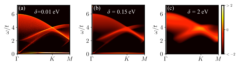
Figure S1: The energy loss function (the imaginary part of the inverse dielectric function ) $1/{\rm Im}[\epsilon^{\text{RPA}}(\bm{q},\omega)]$ on a log scale along the $\Gamma-K-M$ direction for parameters of $J=0.1$ eV, $K=0.1$ eV, $V=6$ eV, $U_{c}=J_{K}=0$ eV, and $U_{f}=20$ eV with variant damping constants $\delta$.

I Disorder effects

In graphene/$\alpha$-RuCl3 heterostructures, the disorder induced by, for instance, impurities and crystal defects are inevitable. This disorder effect usually will impact the lifetime of plasmon excitations. Here, we discuss the qualitative impact of disorder which will effectively result in a very large damping constant $\delta$ when calculating the bare charge susceptibility tensor $\chi^{0}(\bm{q},\omega)$ which explicitly reads

$$\begin{split}&[\chi^{(0)}(\bm{q},\omega)]^{s_{1}s_{1}^{\prime}}_{s_{2}s_{2}^{\prime}}=-\frac{2}{\mathcal{N}}\sum_{\bm{k}\mu\nu}\frac{n_{f}(\omega_{\mu,\bm{k}})-n_{f}(\omega_{\nu,\bm{k+q}})}{\omega_{\mu,\bm{k}}-\omega_{\nu,\bm{k+q}}+\omega+i\delta}[U_{\mu,\bm{k}}^{*}]_{s_{1}}[U_{\nu,\bm{k+q}}]_{s^{\prime}_{1}}[U_{\nu,\bm{k+q}}^{*}]_{s_{2}}[U_{\mu,\bm{k}}]_{s^{\prime}_{2}}.\end{split}$$ (S1)

Here $n_{f}$ is the Fermi function, $\omega_{\mu,\bm{k}}$ is the energy of the $\mu$-th band of quadratic Hamiltonian $H_{0}$ defined in the main text, and $U_{\mu,\bm{k}}$ is the four-component eigenvector associated with energy $\omega_{\mu,\bm{k}}$. In Fig. S1, we plot the energy loss functions for different damping constants $\delta$. In the main text, we usually set the damping constant $\delta\approx{}0.01$ eV. As we can see, a moderately large damping constant of $\delta=0.15$ eV broadens the peak of the energy loss function $1/{\rm Im}[\epsilon^{\text{RPA}}(\bm{q},\omega)]$, i.e., weakening the signals of plasmon excitations. Crucially, the low-energy plasmons will be totally eliminated for strong disorder as shown via a large damping constant of $\delta\approx{}2$ eV, e.g..

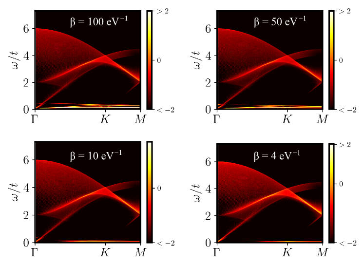
Figure S2: The energy loss function (the imaginary part of the inverse dielectric function ) $1/{\rm Im}[\epsilon^{\text{RPA}}(\bm{q},\omega)]$ on a log scale along the $\Gamma-K-M$ direction for parameters of $J=0.1$ eV, $K=0.1$ eV, $V=6$ eV, $U_{c}=J_{K}=0$ eV, and $U_{f}=20$ eV with different temperatures $\beta$.

II Finite temperature effects

There are two qualitatively different effects of increasing temperature. First and most importantly, the finite temperature effect may destroy the heavy Fermi liquid phase, i.e., the quadratic Hamiltonian $H_{0}$ in the main text with its effective hybridization which allows coupling to the insulating layer. There exists a temperature scale $\beta^{\ast}\approx 4\ {\rm eV}^{-1}$ above which a crossover (manifest as a phase transition in the mean field treatment) from the heavy Fermi liquid phase to the decoupled phase occurs. Notice that the transition temperature $\beta^{*}$ is just a rough estimate and more details can be found in Ref. Seifert et al. (2018). In the decoupled phase, the interlayer hybridization strength is effectively $J=0$ and consequently, the flat plasmon band $\omega_{3}$ and other two emergent bands $\omega^{\prime}_{1}$ and $\omega^{\prime}_{2}$ disappear. Second, within the heavy Fermi liquid phase, increasing temperature will lead to the standard broadening effects from the smearing of the Fermi function. The plasmon bands for different temperatures are shown in Fig. S2, where we have assumed that the interlayer hybridization strength $J$ does not change a lot as a function of temperature within the heavy Fermi liquid phase. We find that finite temperature does not have a significant effect on the plasmon excitations. The flat plasmon band $\omega_{3}$ is still observable for $\beta>4$ eV^-1, whereas the emergent two plasmon bands $\omega^{\prime}_{1}$ and $\omega^{\prime}_{2}$ will gradually disappear around the critical temperature $\beta^{*}\approx 4\ {\rm eV}^{-1}$.

References

- Pines and Bohm (1952) D. Pines and D. Bohm, Phys. Rev. 85, 338 (1952).
- Pines (1956) D. Pines, Rev. Mod. Phys. 28, 184 (1956).
- Millis et al. (1987) A. J. Millis, M. Lavagna, and P. A. Lee, Phys. Rev. B 36, 864 (1987).
- Millis and Coppersmith (1990) A. J. Millis and S. N. Coppersmith, Phys. Rev. B 42, 10807 (1990).
- Freytag and Keller (1990) R. Freytag and J. Keller, Zeitschrift für Physik B Condensed Matter 80, 241 (1990).
- Efimkin and Galitski (2014) D. K. Efimkin and V. Galitski, Phys. Rev. B 90, 081113 (2014).
- van Loon et al. (2014) E. G. C. P. van Loon, H. Hafermann, A. I. Lichtenstein, A. N. Rubtsov, and M. I. Katsnelson, Phys. Rev. Lett. 113, 246407 (2014).
- Greco et al. (2016) A. Greco, H. Yamase, and M. Bejas, Phys. Rev. B 94, 075139 (2016).
- Yin et al. (2019) X. Yin, C. S. Tang, S. Zeng, T. C. Asmara, P. Yang, M. A. Naradipa, P. E. Trevisanutto, T. Shirakawa, B. H. Kim, S. Yunoki, et al., ACS Photonics 6, 3281 (2019).
- Wunsch et al. (2006) B. Wunsch, T. Stauber, F. Sols, and F. Guinea, New Journal of Physics 8, 318 (2006).
- Hwang and Das Sarma (2007) E. H. Hwang and S. Das Sarma, Phys. Rev. B 75, 205418 (2007).
- Bonaccorso et al. (2010) F. Bonaccorso, Z. Sun, T. Hasan, and A. Ferrari, Nature photonics 4, 611 (2010).
- Avouris (2010) P. Avouris, Nano letters 10, 4285 (2010).
- Ju et al. (2011) L. Ju, B. Geng, J. Horng, C. Girit, M. Martin, Z. Hao, H. A. Bechtel, X. Liang, A. Zettl, Y. R. Shen, et al., Nature nanotechnology 6, 630 (2011).
- Koppens et al. (2011) F. H. Koppens, D. E. Chang, and F. J. Garcia de Abajo, Nano letters 11, 3370 (2011).
- Grigorenko et al. (2012) A. Grigorenko, M. Polini, and K. Novoselov, Nature photonics 6, 749 (2012).
- Chen et al. (2012) J. Chen, M. Badioli, P. Alonso-González, S. Thongrattanasiri, F. Huth, J. Osmond, M. Spasenović, A. Centeno, A. Pesquera, P. Godignon, et al., Nature 487, 77 (2012).
- Stauber (2014) T. Stauber, Journal of Physics: Condensed Matter 26, 123201 (2014).
- Eberlein et al. (2008) T. Eberlein, U. Bangert, R. R. Nair, R. Jones, M. Gass, A. L. Bleloch, K. S. Novoselov, A. Geim, and P. R. Briddon, Phys. Rev. B 77, 233406 (2008).
- Kinyanjui et al. (2012) M. K. Kinyanjui, C. Kramberger, T. Pichler, J. C. Meyer, P. Wachsmuth, G. Benner, and U. Kaiser, EPL (Europhysics Letters) 97, 57005 (2012).
- Stauber et al. (2010) T. Stauber, J. Schliemann, and N. M. R. Peres, Phys. Rev. B 81, 085409 (2010).
- Cao et al. (2018a) Y. Cao, V. Fatemi, A. Demir, S. Fang, S. L. Tomarken, J. Y. Luo, J. D. Sanchez-Yamagishi, K. Watanabe, T. Taniguchi, E. Kaxiras, et al., Nature 556, 80 (2018a).
- Cao et al. (2018b) Y. Cao, V. Fatemi, S. Fang, K. Watanabe, T. Taniguchi, E. Kaxiras, and P. Jarillo-Herrero, Nature 556, 43 (2018b).
- Stauber and Kohler (2016) T. Stauber and H. Kohler, Nano letters 16, 6844 (2016).
- Lewandowski and Levitov (2019) C. Lewandowski and L. Levitov, Proceedings of the National Academy of Sciences 116, 20869 (2019).
- Khaliji et al. (2020) K. Khaliji, T. Stauber, and T. Low, Phys. Rev. B 102, 125408 (2020).
- Novelli et al. (2020) P. Novelli, I. Torre, F. H. L. Koppens, F. Taddei, and M. Polini, Phys. Rev. B 102, 125403 (2020).
- Hesp et al. (2019) N. C. H. Hesp, I. Torre, D. Rodan-Legrain, P. Novelli, Y. Cao, S. Carr, S. Fang, P. Stepanov, D. Barcons-Ruiz, H. Herzig-Sheinfux, K. Watanabe, T. Taniguchi, D. K. Efetov, E. Kaxiras, P. Jarillo-Herrero, M. Polini, and F. H. L. Koppens, “Collective excitations in twisted bilayer graphene close to the magic angle,” (2019), arXiv:1910.07893 [cond-mat.str-el] .
- Hu et al. (2017) F. Hu, S. R. Das, Y. Luan, T.-F. Chung, Y. P. Chen, and Z. Fei, Phys. Rev. Lett. 119, 247402 (2017).
- Fahimniya et al. (2020) A. Fahimniya, C. Lewandowski, and L. Levitov, “Dipole-active collective excitations in moiré flat bands,” (2020), arXiv:2011.02982 [cond-mat.mes-hall] .
- Zhou et al. (2019) B. Zhou, J. Balgley, P. Lampen-Kelley, J.-Q. Yan, D. G. Mandrus, and E. A. Henriksen, Phys. Rev. B 100, 165426 (2019).
- Mashhadi et al. (2019) S. Mashhadi, Y. Kim, J. Kim, D. Weber, T. Taniguchi, K. Watanabe, N. Park, B. Lotsch, J. H. Smet, M. Burghard, et al., Nano letters 19, 4659 (2019).
- Wang et al. (2020) Y. Wang, J. Balgley, E. Gerber, M. Gray, N. Kumar, X. Lu, J.-Q. Yan, A. Fereidouni, R. Basnet, S. J. Yun, et al., Nano Letters 20, 8446 (2020).
- Rizzo et al. (2020) D. J. Rizzo, B. S. Jessen, Z. Sun, F. L. Ruta, J. Zhang, J.-Q. Yan, L. Xian, A. S. McLeod, M. E. Berkowitz, K. Watanabe, T. Taniguchi, S. E. Nagler, D. G. Mandrus, A. Rubio, M. M. Fogler, A. J. Millis, J. C. Hone, C. R. Dean, and D. N. Basov, Nano Letters 20, 8438 (2020), pMID: 33166145.
- Kitaev (2006) A. Kitaev, Annals of Physics 321, 2 (2006), january Special Issue.
- Rau et al. (2016) J. G. Rau, E. K.-H. Lee, and H.-Y. Kee, Annual Review of Condensed Matter Physics 7, 195 (2016).
- Winter et al. (2017) S. M. Winter, A. A. Tsirlin, M. Daghofer, J. van den Brink, Y. Singh, P. Gegenwart, and R. Valentí, Journal of Physics: Condensed Matter 29, 493002 (2017).
- Hermanns et al. (2018) M. Hermanns, I. Kimchi, and J. Knolle, Annual Review of Condensed Matter Physics 9, 17 (2018).
- Takagi et al. (2019) H. Takagi, T. Takayama, G. Jackeli, G. Khaliullin, and S. E. Nagler, Nature Reviews Physics 1, 264 (2019).
- Banerjee et al. (2016) A. Banerjee, C. Bridges, J.-Q. Yan, A. Aczel, L. Li, M. Stone, G. Granroth, M. Lumsden, Y. Yiu, J. Knolle, et al., Nature materials 15, 733 (2016).
- Biswas et al. (2019) S. Biswas, Y. Li, S. M. Winter, J. Knolle, and R. Valentí, Phys. Rev. Lett. 123, 237201 (2019).
- Gerber et al. (2020) E. Gerber, Y. Yao, T. A. Arias, and E.-A. Kim, Phys. Rev. Lett. 124, 106804 (2020).
- Choi et al. (2018) W. Choi, P. W. Klein, A. Rosch, and Y. B. Kim, Phys. Rev. B 98, 155123 (2018).
- Seifert et al. (2018) U. F. P. Seifert, T. Meng, and M. Vojta, Phys. Rev. B 97, 085118 (2018).
- Leeb et al. (2021) V. Leeb, K. Polyudov, S. Mashhadi, S. Biswas, R. Valentí, M. Burghard, and J. Knolle, Phys. Rev. Lett. 126, 097201 (2021).
- (46) See the Supplemental Material for more details .
- Schrieffer et al. (1989) J. R. Schrieffer, X. G. Wen, and S. C. Zhang, Phys. Rev. B 39, 11663 (1989).
- Chubukov and Frenkel (1992) A. V. Chubukov and D. M. Frenkel, Phys. Rev. B 46, 11884 (1992).
- Knolle et al. (2010) J. Knolle, I. Eremin, A. V. Chubukov, and R. Moessner, Phys. Rev. B 81, 140506 (2010).
- Stauber (2010) T. Stauber, Phys. Rev. B 82, 201404 (2010).
- Hill et al. (2009) A. Hill, S. A. Mikhailov, and K. Ziegler, EPL (Europhysics Letters) 87, 27005 (2009).
- Note (1) For illustration purposes and imposing the local constraint of Abrikosov fermions, we have used very large Hubbard repulsion to demonstrate and . These two bands do not qualitatively change as increases, and the higher order corrections Sodemann and Fogler (2012) must be considered to quantitatively determine and .
- Atkin et al. (2012) J. M. Atkin, S. Berweger, A. C. Jones, and M. B. Raschke, Advances in Physics 61, 745 (2012).
- Basov et al. (2016) D. N. Basov, M. M. Fogler, and F. J. García de Abajo, Science 354 (2016), 10.1126/science.aag1992.
- Low et al. (2017) T. Low, A. Chaves, J. D. Caldwell, A. Kumar, N. X. Fang, P. Avouris, T. F. Heinz, F. Guinea, L. Martin-Moreno, and F. Koppens, Nature materials 16, 182 (2017).
- Sunku et al. (2018) S. S. Sunku, G. X. Ni, B. Y. Jiang, H. Yoo, A. Sternbach, A. S. McLeod, T. Stauber, L. Xiong, T. Taniguchi, K. Watanabe, P. Kim, M. M. Fogler, and D. N. Basov, Science 362, 1153 (2018).
- Ni et al. (2015) G. Ni, H. Wang, J. Wu, Z. Fei, M. Goldflam, F. Keilmann, B. Özyilmaz, A. C. Neto, X. Xie, M. Fogler, et al., Nature materials 14, 1217 (2015).
- Woessner et al. (2015) A. Woessner, M. B. Lundeberg, Y. Gao, A. Principi, P. Alonso-González, M. Carrega, K. Watanabe, T. Taniguchi, G. Vignale, M. Polini, et al., Nature materials 14, 421 (2015).
- Dai et al. (2015) S. Dai, Q. Ma, M. Liu, T. Andersen, Z. Fei, M. Goldflam, M. Wagner, K. Watanabe, T. Taniguchi, M. Thiemens, et al., Nature nanotechnology 10, 682 (2015).
- Wu et al. (2015) J.-S. Wu, D. N. Basov, and M. M. Fogler, Phys. Rev. B 92, 205430 (2015).
- Hwang et al. (2010) E. H. Hwang, R. Sensarma, and S. Das Sarma, Phys. Rev. B 82, 195406 (2010).
- Park et al. (2020) J. Y. Park, J. Jo, J. A. Sears, Y.-J. Kim, M. Kim, P. Kim, and G.-C. Yi, Phys. Rev. Materials 4, 113404 (2020).
- Hwang et al. (2018) J. Hwang, K. Kim, H. Ryu, J. Kim, J.-E. Lee, S. Kim, M. Kang, B.-G. Park, A. Lanzara, J. Chung, et al., Nano letters 18, 3661 (2018).
- Sodemann and Fogler (2012) I. Sodemann and M. M. Fogler, Phys. Rev. B 86, 115408 (2012).