Information entropy in AdS/QCD: mass spectroscopy of isovector mesons

Abstract

The mass spectra of isovector $\Upsilon$, $\psi$, $\phi$, and $\omega$ meson resonances are investigated, in the AdS/QCD and information entropy setups. The differential configurational entropy is employed to obtain the mass spectra of radial $S$-wave resonances, with higher excitation levels, in each one of these meson families, whose respective first undisclosed states are discussed and matched up to candidates in the Particle Data Group.

I Introduction

In Shannon’s theory, the information entropy of some random variable consists of the average level of information that is inherent to the possible outcomes of this variable Shannon:1948zz . It can be performed by the theory configurational entropy (CE), which comprises the amount of entropy endowing a discrete system that governs correlations among its constituents. The CE estimates how information can be encrypted in wave modes, in momentum space, still describing the whole system under scrutiny. The maximal CE is attained by a source having a probability distribution that is uniform and, in this way, uncertainty attains the maximal value in the case of equiprobable events. When one takes the continuous limit, the differential configurational entropy (DCE) plays the role of the CE, once the information dimension vanishes Bernardini:2016hvx . The DCE has been employed to study physical systems in a variety of circumstances Gleiser:2018kbq ; Gleiser:2011di ; Gleiser:2012tu , once a localized scalar field that portrays the system is taken into account Karapetyan:2018oye ; Karapetyan:2018yhm .

In the precise context of AdS/QCD, the DCE has been playing a prominent role in the investigation of hadrons, estimating new features of hadronic states in AdS/QCD Bernardini:2018uuy ; Ferreira:2019inu ; daRocha:2021imz ; Ferreira:2019nkz and also corroborating to existing hadronic properties. Recent studies in the DCE setup of AdS/QCD investigated light-flavor mesons, heavy mesons encompassing charmonia and bottomonia resonances, tensorial mesons, baryons, glueball fields, pomerons, odderons, and baryons, including finite-temperature regimes Colangelo:2018mrt ; Ferreira:2020iry ; Braga:2018fyc ; Braga:2020myi ; Braga:2020hhs ; MarinhoRodrigues:2020yzh ; Bernardini:2016qit ; Braga:2017fsb ; Karapetyan:2016fai ; Karapetyan:2017edu ; Karapetyan:2019ran ; Karapetyan:2019fst ; Karapetyan:2020yhs ; Barbosa-Cendejas:2018mng ; Ma:2018wtw . Some of the obtained results were confirmed by the Particle Data Group (PDG) pdg and also matched up to new meson candidates that were previously unattached to some of the studied meson families. Other relevant implementations of the DCE paradigm in QFT and AdS/CFT were reported in Refs. Correa:2015vka ; Correa:2016pgr ; Cruz:2019kwh ; Lee:2019tod ; Bazeia:2018uyg ; Bazeia:2021stz ; Alves:2014ksa ; Alves:2017ljt ; Gleiser:2018jpd ; Braga:2019jqg ; Braga:2020opg ; Casadio:2016aum ; Fernandes-Silva:2019fez ; Bernardini:2019stn ; Lee:2018zmp ; Thakur:2020sko .

With the aid of data from experiments and theoretical developments, meson spectroscopy composes a paradigm asserting that mesons present ubiquitous features. Important studies support universal properties that include all the meson spectrum, running from light-flavor ones to heavy charmonium and bottomonium amsler ; Simonov:1989fd ; Badalian:2016ttl ; Frederico:2014bva ; dePaula:2009za . Meson spectroscopy has been successfully scrutinized in the context of the AdS/QCD duality. In this setup, there is an AdS bulk that places a weakly-coupled gravity sector, which is the dual theory of conformal field theory (CFT) living on the codimension one AdS boundary. In the duality, physical fields that reside in the bulk are equivalent to operators in strongly-coupled QCD on the AdS boundary. The bulk extra dimension implements the QCD energy scale Csaki ; Karch:2006pv ; Branz:2010ub . Among possible models endowing AdS/QCD, the soft wall prescribes Regge trajectories to come out from confinement, being implemented by a dilaton that is a quadratic function of the energy scale Colangelo:2008us ; MartinContreras:2020cyg . Linear Regge trajectories successfully describe the mass spectrum of light-flavor meson families, at least when considering the radial $S$-wave resonances that have not so high excitation $n$ levels. The range wherein the linearity holds can vary for each light-flavor meson family. When hadronic states are constituted by strange, charm, bottom, or top quarks, the linear regime $m_{n}^{2}\propto n$ is no longer verified MartinContreras:2020cyg ; Afonin:2014nya . The Bohr–Sommerfeld quantization technique applied to the Salpeter-like equation was used to derive nonlinear Regge trajectories for meson states constituted by distinct quarks, presenting similar profiles as the ones for quarkonia MartinContreras:2020cyg , complying with experimental data and also to the theoretical predictions Chen:2018nnr . Besides, due to the chasm among the heavy and light quark masses, more recent models regard massive quarks that constitute mesons. Therefore, more realistic scenarios can encompass nonlinear Regge trajectories, induced by the quark constituent mass. Light-flavor quarks comprehend up, down, and strange ones, that are much less massive than heavy quarks as the bottom, charm, and top ones. Heavy quarks can form quarkonia, as the $J/\psi$ meson ground state, and the $\Upupsilon$ mesons as well.

Isovector mesons are characterized by the isobaric spin $I^{G}=0^{-}$ with negative $G$-parity, and unit total angular momentum $J^{PC}=1^{--}$, with both parity ($P$) and charge conjugation ($C$) negative quantum numbers. Isovector mesons encompass $\Upupsilon$ mesons, consisting of a quarkonium state – the bottomonium – formed by a bottom quark ($b$) and its antiparticle ($\bar{b}$); $\phi$ mesons, formed of a strange quark and a strange antiquark; $\psi$ mesons, consisting of a charm quark ($c$) and a charm antiquark ($\bar{c}$) and forming charmonia states; and $\omega$ mesons as bound states of up and down quarks, with their correspondent antiquarks. The top quark has a much bigger mass when compared to the other quarks, being five orders of magnitude more massive than the up and down quarks and two orders of magnitude more massive than the bottom and charm heavy quarks. Although toponium, formed by a top quark ($t$) and its antiquark ($\bar{t}$) is more difficult to detect since top quarks decay through the electroweak gauge force before bound states set in, there are recently reported signatures of toponium formation by gluon fusion, in the LHC run 2 data Fuks:2021xje . Contrary to bottomonium and charmonium, toponium resonances decay instantly, as $t$ and $\bar{t}$ have a $5\times 10^{-25}$ s lifetime. Toponium has also a huge decay width.

In this work, the DCE of the isovector mesons families will be computed, as a function of both the radial $S$-wave resonances excitation level and their experimental mass spectra as well. Hence, the mass spectra of radial $S$-wave resonances with higher excitation levels can be obtained. It is accomplished when plotting the associated graphics and, when interpolating them, two types of DCE Regge trajectories can be then produced. The first ones relate the DCE to the radial $S$-wave resonances, whereas the second ones associate the DCE with the isovector families experimental mass spectra. Working with the polynomial interpolation formulæ  of each interpolation curve for the four families of isovector mesons ($\Upupsilon$, $\psi$, $\omega$, and $\phi$) yields the mass spectra of higher $n$ resonances in these families. They comprise candidates in the next generations proposed to be detected in experiments, as well as candidates that match up to states in PDG pdg .

This work is organized as follows: Sec. II is dedicated to introducing the basics on AdS/QCD, with a deviation from the soft wall dilaton background that is induced by the massive quarks that constitute isovector mesons. This emulates the standard soft wall when the deviation parameter equals zero and encompasses the light-flavor meson states with massless constituent quarks, in this limit. The mass spectra of isovector $\Upupsilon$, $\psi$, $\phi$, and $\omega$ meson resonances are then derived. Sec. III is hence devoted to the essentials of the DCE setup. The DCE of the isovector $\Upupsilon$, $\psi$, $\phi$, and $\omega$ meson families is calculated as a function of both the radial $S$-wave resonances excitation level and their experimental mass spectra. Extrapolating both DCE Regge trajectories yields the mass spectra of heavier isovector resonances in each one of the $\Upupsilon$, $\psi$, $\phi$, and $\omega$ meson families, whose first undisclosed states are analyzed and matched up to existing candidates in PDG. In particular, a precise mass spectrum of bottomonia and charmonia is derived. Sec. IV encloses discussion, analysis, and relevant perspectives.

II AdS/QCD fundamentals

Isovector mesons are represented, in the soft wall model Karch:2006pv , by a vector field $V_{M}=(V_{\mu},V_{z})\,$ where greek indexes run from $0$ to $3$, living in AdS space. These fields can be thought of as being dual objects that correspond to the current density ${\rm J}^{\mu}(x)=\bar{q}(x)\upgamma^{\mu}q(x)$ in the CFT on the boundary, where $q(x)$ denote quark fermionic fields and $\upgamma^{\mu}$ stand for the gamma Dirac matrices, whereas here $\bar{q}(x)\equiv{q}^{\dagger}(x)\upgamma^{0}$. These vector field are governed by the action

$$I\,=-\frac{1}{g_{5}^{2}}\int dz\,{\rm d}^{4}x\,\sqrt{-g}\,\,\mathcal{L},$$ (1)

where

$$\mathcal{L}=\frac{1}{4}\,e^{-\upphi(z)}F^{*}_{MN}F^{MN}$$ (2)

denotes the Lagrangian and $F_{MN}=\mbox{\hskip 5.30904pt{1 0 -.25 1}\hbox to0.0pt{\hss\leavevmode\hbox{\set@color$\partial$}}}\kern-0.8pt_{M}V_{N}-\mbox{\hskip 5.30904pt{1 0 -.25 1}\hbox to0.0pt{\hss\leavevmode\hbox{\set@color$\partial$}}}\kern-0.8pt_{N}V_{M}$. The AdS bulk is equipped with the metric

$$ds^{2}=g_{MN}dx^{M}dx^{N}=e^{2A(z)}(\upeta_{\mu\nu}dx^{\mu}dx^{\nu}+dz^{2})\,,$$ (3)

with warp factor ${A}(z)=-\log(z/R)$, where $\upeta_{\mu\nu}$ denotes the boundary metric.

Ref. MartinContreras:2020cyg proposed a deviation for the soft wall standard quadratic dilaton,

$$\upphi(z)=(\upkappa z)^{2-\upalpha},$$ (4)

where the energy parameter $\upkappa$ is related to the mass scale and $\upalpha$ is the shift parameter driven by constituent massive quarks. Leading $\upalpha$ to zero, light-flavor mesons with massless constituent quarks are recovered, emulating the standard AdS/QCD soft wall.

Using (1) and imposing the gauge where $V_{z}=0$ yields an EOM ruling the bulk field

$$\left[\mbox{\hskip 5.30904pt{1 0 -.25 1}\hbox to0.0pt{\hss\leavevmode\hbox{\set@color$\partial$}}}\kern-0.8pt_{z}^{2}-B^{\prime}(z)\mbox{\hskip 5.30904pt{1 0 -.25 1}\hbox to0.0pt{\hss\leavevmode\hbox{\set@color$\partial$}}}\kern-0.8pt_{z}-q^{2}\right]V_{\mu}(z,q)=0,$$ (5)

where $B(z)=\upphi(z)-A(z)$ and the prime denotes the derivative with respect to $z$. The bulk isovector field can be split off as

$$V_{\mu}(z,q)=V_{\mu}(q)\,\xi(z,q),$$ (6)

where $\xi(z,q)$ denotes the bulk-to-boundary propagator. Hence, the EOM ruling the bulk isovector field is led to a Schrödinger-like equation. The Bogoliubov mapping $\xi(z,q)=e^{\upphi(z)/2}\upxi(z,q)$ yields MartinContreras:2020cyg

$$\left[-\mbox{\hskip 5.30904pt{1 0 -.25 1}\hbox to0.0pt{\hss\leavevmode\hbox{\set@color$\partial$}}}\kern-0.8pt_{z}^{2}+U(z)\right]\,\upxi(z,q)=-q^{2}\upxi(z,q),$$ (7)

with the potential

$$U(z) = -\frac{1}{2}B^{\prime\prime}(z)+\frac{1}{4}B^{\prime 2}(z).$$ (8)

For the term $V_{\mu}(q)$, defined in the splitting (6) to correspond to the source of the correlators of gauge theory current densities, one must impose the Dirichlet boundary condition $\lim_{z\to 0}\xi(z,q)=1$. The CFT boundary value of the vector field $V_{\mu}(q)\equiv\lim_{z\to 0}V_{\mu}(z,q)$ emulates a source that generates correlators of the boundary current operator ${\rm J}^{\mu}(x)$

$$\!\!\langle\,0\,|\,{\rm J}_{\mu}(x){\rm J}_{\nu}(x^{\prime})\,|\,0\,\rangle=\frac{\updelta}{\updelta V_{\mu}(x)}\frac{\updelta}{\updelta V_{\nu}(x^{\prime})}e^{-I_{\scalebox{0.59}{{on-shell}}}},$$ (9)

where $I_{\scalebox{0.64}{{on-shell}}}$ denotes the on-shell action, obtained by the boundary term

$$\!\!\!\!\!\!\!\!I_{\scalebox{0.64}{{on-shell}}}\!=\!-\frac{1}{2\mathring{g}_{5}^{2}}\lim_{z\to 0}\left[\int{\rm d}^{4}x\,\,\frac{1}{z}{e^{-(\upkappa z)^{2-\upalpha}}V_{\nu}\mbox{\hskip 5.30904pt{1 0 -.25 1}\hbox to0.0pt{\hss\leavevmode\hbox{\set@color$\partial$}}}\kern-0.8pt_{z}V^{\nu}}\right],$$ (10)

for $\mathring{g}_{5}^{2}={g_{5}^{2}}/{R}$. Eq. (10) generalizes, for the deviated quadratic dilaton (4), the results that take into account the quadratic dilaton Braga:2015jca . The correlator reads

$$\!\Pi(q^{2})\!=\!-\frac{1}{\mathring{g}_{5}^{2}q^{2}}\lim_{z\to 0}\left[\frac{1}{z}e^{-(\upkappa z)^{2-\upalpha}}\xi(z,q)\mbox{\hskip 5.30904pt{1 0 -.25 1}\hbox to0.0pt{\hss\leavevmode\hbox{\set@color$\partial$}}}\kern-0.8pt_{z}\xi(z,q)\right]\,.$$ (11)

The AdS/QCD correspondence asserts that mesonic states can be established through the conformal dimension $\Updelta$ playing the role of a scaling dimension. The Regge angle for a given mesonic trajectory is defined by the dilaton energy scale $\upkappa$. Bulk fields are dual objects to an $\mathbb{O}$ operator that is driven by the CFT on the AdS boundary, whose correlator is given by $\left\langle\mathbb{O}(x^{\mu})\,\mathbb{O}(\mathbf{0})\right\rangle\propto\|\,x^{\mu}\,\|^{-2\Updelta}$ Witten:1998qj . The spin $S$, the bulk mass, $\mathbb{M}$, and the conformal dimension, $\Updelta$, are fine-tuned by the following expression Witten:1998qj ,

$$\mathbb{M}_{5}^{2}R^{2}=(\Updelta-S)(\Updelta+S-4).$$ (12)

Eq. (12) holds for the $S$-wave, $\ell=0$, approach of isovector mesons, with $\Updelta=3$ and $S=1$.

Eq. (7) yields the mass spectrum $m_{n}^{2}=-q^{2}$ of isovector mesons states, with radial excitation level $n$, as eigenvalues of the Schrödinger-like operator. When replacing the shift of the standard quadratic dilaton (4) in the potential (8) yields MartinContreras:2020cyg

$$\!\!\!\!\!\!\!\!\!\!\!U(z,\upkappa,\upalpha)\! \!=\! \!\frac{3}{4z^{2}}+\left(\frac{3\upalpha}{2}-\frac{\upalpha^{2}}{2}-\upkappa^{2}\right)\upkappa^{2}(\upkappa z)^{-\upalpha}$$ (13)

$$\!+\! \!\!\frac{\upkappa^{2}}{4}\left(\upalpha\!-\!2\right)^{2}\!(\upkappa z)^{2-2\upalpha}\!+\!\frac{\upkappa}{z}\left(1\!-\!\frac{\upalpha}{2}\right)\!(\upkappa z)^{1\!-\!\upalpha}.$$

If the quarks that constitute the isovector mesons are taken in the massless limit, corresponding to $\upalpha=0$, the potential (13) leads to the vector meson fields Karch:2006pv . The parameter $\upalpha$ encodes the massive quarks constituents and their flavor within isovector mesons MartinContreras:2020cyg . Different isovector meson states, with different masses and radial quantum numbers, are distinguished when one adopts, as usual, eigenvalues $-q^{2}=m_{n}^{2}=4\kappa^{2}n$, for $n=1,2,3,\ldots$, corresponding to the mass spectrum derived in Eq. (7). Different radial excitation levels $n$ yield different mesonic excitations in each one of the isovector meson families.

To obtain the radial $S$-wave resonances of the isovector families, the generalized potential in Eq. (13) must be substituted into Eq. (7) , whose numerical solutions, for the isovector meson families, are encoded in Tables 1 – 4, with the $\upkappa$ and $\upalpha$ parameters that are appropriate to fit the mass spectra of each isovector meson family, respectively MartinContreras:2020cyg . It is worth to emphasize that to fit the mass spectra of the four isovector meson families, appropriate values of the two parameters $\upalpha$ and $\upkappa$ must be chosen. For the $\Upupsilon$ meson family, the values $\upalpha=0.863$ and $\upkappa=11.209$ GeV best fit the experimental data, whereas $\upalpha=0.541$ and $\upkappa=2.150$ GeV are more suitable for describing the family of $\psi$ isovector mesons. Besides, the $\omega$ meson family is best described by adopting $\upalpha=0.040$ and $\upkappa=0.498$ GeV, and to match the mass spectrum of $\phi$ isovector mesons requires $\upalpha=0.070$ and $\upkappa=0.585$ GeV.

————–  $\Upupsilon$ mesons mass spectrum  —————

$n$	State	$M_{\scalebox{0.67}{{Experimental}}}$ (MeV)	$M_{\scalebox{0.67}{{Theory}}}$ (MeV)
1	$\Upupsilon(1S)\;$	$9460.30\pm 0.26$	9438.51
2	$\Upupsilon(2S)\;$	$10023.26\pm 0.32$	9923.32
3	$\Upupsilon(3S)\;$	$10355\pm 0.5$	10277.2
4	$\Upupsilon(4S)\!=\!\Upupsilon(10580)\;$	$10579.4\pm 1.2$	10558.6
5	$\Upupsilon(10860)\;$	$10889.9^{+3.2}_{-2.6}$	10793.5
6	$\Upupsilon(11020)\;$	$11000\pm 4$	10995.7

Table 1: Experimental and theoretical mass spectrum of $S$-wave resonances in the $\Upupsilon$ meson family. For the masses in the fourth column, obtained by solving Eq. (7), $\upalpha=0.863$ and $\upkappa=11.209$ GeV.

In particular regarding Table 1, some issues on the heavier bottomonia, which were detected around a quarter of a century ago, still consist of a conundrum in QCD. Thorough investigations concerning the $\Upupsilon$ meson family, involving the in-depth analysis of available data provided by CLEO, CUSB, and BaBar collaborations, have been accomplished pdg ; Besson:1984bd ; Chen:2016mjn . It is worth emphasizing that the $\Upupsilon(10580)$ resonance is the bottomonium state of lowest mass, that is above the so-called open-bottom threshold, that decays into two mesons that are composed by a bottom antiquark and either an up, a down, a strange, or a charm quark, originating respectively the $B^{+}$, $B^{0}$, $B^{0}_{s}$, and $B^{+}_{c}$ mesons Aubert:2004pwa .

————–  $\psi$ mesons mass spectrum  —————

$n$	State	$M_{\scalebox{0.67}{{Experimental}}}$ (MeV)	$M_{\scalebox{0.67}{{Theory}}}$ (MeV)
1	$J/\psi(1S)\;$	$3096.900\pm 0.006$	3077.09
2	$\psi(2S)\;$	$3686.10\pm 0.06$	3689.62
3	$\psi(4040)\;$	$4039\pm 1$	4137.5
4	$\psi(4415)\;$	$4421\pm 4$	4499.4
5	$\psi(4660)\;$	$4633\pm 7$	4806.3

Table 2: Experimental and theoretical mass spectrum of $S$-wave resonances in the $\psi$ meson family. For the masses in the fourth column, obtained by solving Eq. (7), $\upalpha=0.541$ and $\upkappa=2.150$ GeV.

Regarding Tables 2 and 3, Belle, CDF, and LHCb collaborations produced relevant data, in particular about the $\omega$ resonances, whose narrow width can induce relevant effects of scattering involving the $J/\psi$, $\omega$, and charmonium Braaten:2013poa .

————–  $\omega$ mesons mass spectrum  —————

$n$	State	$M_{\scalebox{0.67}{{Experimental}}}$ (MeV)	$M_{\scalebox{0.67}{{Theory}}}$ (MeV)
1	$\omega(782)\;$	$782.65\pm 0.12$	981.43
2	$\omega(1420)\;$	$1410\pm 60$	1374
3	$\omega(1650)\;$	$1670\pm 30$	1674
4	$\omega(1960)\;$	$1960\pm 25$	1967
5	$\omega(2205)\;$	$2205\pm 30$	2149
6	$\omega(2290)\;$	$2290\pm 20$	2348

Table 3: Experimental and theoretical mass spectrum of $S$-wave resonances in the $\omega$ meson family. For the masses in the fourth column, obtained by solving Eq. (7), $\upalpha=0.040$ and $\upkappa=0.498$ GeV.

————–  $\phi$ mesons mass spectrum  —————

$n$	State	$M_{\scalebox{0.67}{{Experimental}}}$ (MeV)	$M_{\scalebox{0.67}{{Theory}}}$ (MeV)
1	$\phi(1020)\;$	$1019.461\pm 0.016$	1139.43
2	$\phi(1680)\;$	$1680\pm 20$	1583
3	$\phi(2170)\;$	$2160\pm 80$	2204

Table 4: Experimental and theoretical mass spectrum of the $S$-wave resonances in the $\phi$ meson family. For the masses in the fourth column, obtained by solving Eq. (7), $\upalpha=0.070$ and $\upkappa=0.585$ GeV.

Data in Tables 1 – 4 are displayed in Figs. 1 and 2.

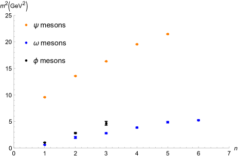
Figure 1: Experimental squared mass spectrum of the isovector meson families, with respect to the $S$-wave resonances excitation levels, $n$, with error bars. The orange points correspond to the $\psi$ meson family, for $n=1,\ldots,5$, respectively coinciding to the $J/\psi(1S)$, $\psi(2S)$, $\psi(4040)$, $\psi(4415)$, and $\psi(4660)$ $S$-wave resonances; the blue points regards the $\omega$ meson family, for $n=1,\ldots,6$, respectively corresponding to the $\omega(782)$, $\omega(1420)$, $\omega(1650)$, $\omega(1960)$, $\omega(2205)$, and $\omega(2290)$ $S$-wave resonances; and the black points depict the $\phi$ meson family, for $n=1,\ldots,3$, respectively corresponding to the $\phi(1020)$, $\phi(1680)$, and $\phi(2170)$ $S$-wave resonances in PDG pdg .

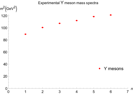
Figure 2: Experimental squared mass spectrum of the $\Upupsilon$ family, for $n=1,\ldots,6$, with error bars, respectively corresponding to the $\Upupsilon(1S)$, $\Upupsilon(2S)$, $\Upupsilon(3S)$, $\Upupsilon(4S)=\Upupsilon(10580)$, $\Upupsilon(10860)$, and $\Upupsilon(11020)$ $S$-wave resonances in PDG pdg .

III Mass spectroscopy of isovector mesons from DCE

The DCE quantifies the correlations out of the oscillations of energy configurations associated with physical systems under scrutiny. For it, the energy density, namely the temporal $\tau_{00}({\bf r})$ component of the stress-energy tensor field, for ${\bf r}=(x_{1},\ldots,x_{k})\in\mathbb{R}^{k}$, emulates a measurable Lebesgue-integrable localized scalar field. The correlator

$$\Uppi({\bf r})=\int_{\mathbb{R}^{k}}{\rm d}^{k}x\,\tau_{00}(\mathring{\bf r})\tau_{00}(\mathring{\bf r}+{\bf r})$$ (14)

sets the DCE to be thought of as the Shannon’s information entropy that regulates the correlations among the system constituents Braga:2018fyc . Now denoting by ${\bf q}$ the spatial part of the 4-momentum $q$, the protocol to derive the DCE has a first step of computing the Fourier transform,

$$\tau_{00}({\bf q})=\frac{1}{(2\pi)^{k/2}}\int_{\mathbb{R}^{k}}{\rm d}^{k}x\,\tau_{00}({\bf r})e^{-i{\bf q}\cdot{\bf r}}.$$ (15)

Any given wave mode enclosed by a $k$-volume ${\rm d}^{k}{q}$, which has center at ${\bf q}$, is related to a probability, $\mathcal{P}$, corresponding to the spectral density in the given wave mode, that reads Gleiser:2018kbq

$$\mathcal{P}\left({\bf q}\,|\,{\rm d}^{k}q\right)\propto\left|\tau_{00}({\bf q})\right|^{2}{\rm d}^{k}q.$$ (16)

The probability distribution (15) engenders the modal fraction Gleiser:2012tu ,

$$\uptau_{00}({\bf q})=\frac{\left|\tau_{00}({\bf q})\right|^{2}}{\int_{\mathbb{R}^{k}}\,{\rm d}^{k}{q}\,\left|\tau_{00}({\bf q})\right|^{2}}.$$ (17)

The weight of information that is necessary to encode $\tau_{00}$, with respect to wave modes, is calculated by the DCE,

$${\rm DCE}_{\tau_{00}}=-\int_{\mathbb{R}^{k}}\,{\rm d}^{k}q\,{\uptau_{00}^{\scalebox{0.73}{$\,\triangleright$}}}({\bf q})\log{\uptau_{00}^{\scalebox{0.73}{$\,\triangleright$}}}({\bf q})\,,$$ (18)

where $\uptau_{{00}}^{\scalebox{0.73}{$\,\triangleright$}}({\bf q})=\uptau_{00}({\bf q})/\uptau_{{00}}^{\scalebox{0.68}{sup}}({\bf q})$, and ${\uptau_{{00}}^{\scalebox{0.68}{sup}}({\bf q})}$ denotes the supremum value of $\uptau_{00}$ attained in $\mathbb{R}^{k}$. Besides, in the state ${\uptau_{{00}}^{\scalebox{0.68}{sup}}({\bf q})}$, the spectral density reaches its highest value. The DCE is measured in terms of nat/unit volume. The acronym nat designates the information natural unit, where nat${}^{-1}=\log 2$/bits. It is equivalent to the information of a uniform probability distribution in the interval of the real line between the origin and the Euler’s number. The DCE encrypts the information of scale, since the spectral density is represented by the Fourier transform of the correlator Gleiser:2018kbq .

To compute the DCE of isovector families, $k=1$ is chosen in Eqs. (15) – (18), since the CFT boundary has codimension one. Replacing the Lagrangian (2) into the stress-energy tensor field expression,

$${\!\!\!\!\!\!\!\!\tau_{00}\!=\!\frac{2}{\sqrt{-g}}\!\!\left[\frac{\mbox{\hskip 5.30904pt{1 0 -.25 1}\hbox to0.0pt{\hss\leavevmode\hbox{\set@color$\partial$}}}\kern-0.8pt(\sqrt{-g}{\mathcal{L}})}{\mbox{\hskip 5.30904pt{1 0 -.25 1}\hbox to0.0pt{\hss\leavevmode\hbox{\set@color$\partial$}}}\kern-0.8pt{g^{00}}}\!-\!\frac{\mbox{\hskip 5.30904pt{1 0 -.25 1}\hbox to0.0pt{\hss\leavevmode\hbox{\set@color$\partial$}}}\kern-0.8pt}{\mbox{\hskip 5.30904pt{1 0 -.25 1}\hbox to0.0pt{\hss\leavevmode\hbox{\set@color$\partial$}}}\kern-0.8pt{x^{\beta}}}\frac{\mbox{\hskip 5.30904pt{1 0 -.25 1}\hbox to0.0pt{\hss\leavevmode\hbox{\set@color$\partial$}}}\kern-0.8pt(\sqrt{-g}{\mathcal{L}})}{\mbox{\hskip 5.30904pt{1 0 -.25 1}\hbox to0.0pt{\hss\leavevmode\hbox{\set@color$\partial$}}}\kern-0.8pt\left(\frac{{\scalebox{0.79}{$\,\mbox{\hskip 3.71632pt{1 0 -.25 1}\hbox to0.0pt{\hss\leavevmode\hbox{\set@color$\partial$}}}\kern-0.8pt$}}g^{00}}{{\scalebox{0.79}{$\,\mbox{\hskip 3.71632pt{1 0 -.25 1}\hbox to0.0pt{\hss\leavevmode\hbox{\set@color$\partial$}}}\kern-0.8pt$}}x^{\beta}}\right)}\right]},$$ (19)

and subsequently computing its Fourier transform, the modal fraction, and the DCE, respectively using Eqs. (15) – (18), we can derive the mass spectra of the isovector meson families. The energy density can be then written as

$$\!\!\!\!\!\!\tau_{00}\!=\!f(\upkappa,\upalpha)g_{00}\left(g^{MP}g^{NQ}F_{MN}F_{PQ}\right)\!-\!g^{MN}F_{0M}F_{0N},$$ (20)

for $P,Q=0,1,2,3,5$, denoting $f(\upkappa,\upalpha)={e^{-(\upkappa z)^{2-\upalpha}}}/{4g_{5}^{2}}$. Now when a plane wave solution is considered in the isovector meson rest frame $V_{\mu}=\epsilon_{\mu}\xi(q,z)e^{-imc^{2}t}$, without loss of generality, the polarization $\epsilon_{\mu}=(0,1,0,0)^{\intercal}$ yields

$$\!\!\!\!\!\tau_{00}=\frac{z^{2}e^{-(\upkappa z)^{2-\upalpha}}}{2g_{5}^{2}R^{2}}\left[-\left(\mbox{\hskip 5.30904pt{1 0 -.25 1}\hbox to0.0pt{\hss\leavevmode\hbox{\set@color$\partial$}}}\kern-0.8pt_{z}\xi\right)^{2}+m_{n}^{2}\xi^{2}\right],$$ (21)

again stressing the fact that $m_{n}^{2}=4\kappa^{2}n$, for $n=1,2,3,\ldots$, determines the mass spectra for different isovector meson states.

This technique, taking into account the information content of AdS/QCD, based on the interpolation of the experimental mass spectra of the four families of isovector mesons in PDG pdg , is more precise when compared to just solving Eq. (7) to derive the mass spectra. The DCE, using the protocol (15 – 18), for each isovector meson family, is numerically calculated and exhibited in Tables 5 – 8.

$n$	State	DCE (nat)
1	$\Upupsilon(1S)\;$	24.78
2	$\Upupsilon(2S)\;$	26.71
3	$\Upupsilon(3S)\;$	28.30
4	$\Upupsilon(4S)=\Upupsilon(10580)\;$	29.88
5	$\Upupsilon(10860)\;$	31.92
6	$\Upupsilon(11020)\;$	33.96

Table 5: DCE of the $S$-wave resonances in the $\Upupsilon$ meson family.

$n$	State	DCE (nat)
1	$J/\psi(1S)\;$	19.45
2	$\psi(2S)\;$	20.81
3	$\psi(4040)\;$	22.07
4	$\psi(4415)\;$	23.97
5	$\psi(4660)\;$	25.64

Table 6: DCE of the $S$-wave resonances in the $\psi$ meson family.

$n$	State	DCE (nat)
1	$\omega(782)\;$	11.37
2	$\omega(1420)\;$	12.46
3	$\omega(1650)\;$	13.51
4	$\omega(1960)\;$	15.14
5	$\omega(2205)\;$	17.36
6	$\omega(2290)\;$	18.69

Table 7: DCE of the $S$-wave resonances in the $\omega$ meson family.

$n$	State	DCE (nat)
1	$\phi(1020)\;$	13.48
2	$\phi(1680)\;$	15.39
3	$\phi(2170)\;$	17.52

Table 8: DCE of the $S$-wave resonances in the $\phi$ meson family.

The first form of DCE Regge trajectories regards the DCE with respect to the $n$ radial excitation level of isovector meson resonances. Fig. 3 shows the obtained outcomes, whose cubic polynomial interpolation of data in Tables 5 – 8 respectively generates the first type of DCE Regge trajectories,

$$\!\!\!\!\!\!\!\!\!\!\!\!{\color[rgb]{0,0,0}_{\Upupsilon}(n)}\!\! \!=\! {\color[rgb]{0,0,0}4.196\times 10^{-2}n^{2}+1.509n+23.339},$$ (22a)

$$\!\!\!\!\!\!\!\!\!\!\!\!\!{\color[rgb]{0,0,0}_{\psi}(n)}\!\! \!= {\color[rgb]{0,0,0}0.090n^{2}+1.014n+18.356},$$ (22b)

$$\!\!\!\!\!\!\!\!\!\!\!\!\!{\color[rgb]{0,0,0}_{\omega}(n)}\!\! \!=\! {\color[rgb]{0,0,0}0.132n^{2}+0.632n+10.591},$$ (22c)

$$\!\!\!\!\!\!\!\!\!\!\!\!\!{\color[rgb]{0,0,0}_{\phi}(n)}\!\! \!=\! \!{\color[rgb]{0,0,0}0.110n^{2}+1.580n+11.790},$$ (22d)

within $1\%$ ($\Upupsilon$ and $\psi$), $1.2\%$ ($\omega$), and $0.2\%$ ($\phi$) root-mean-square deviation (RMSD).

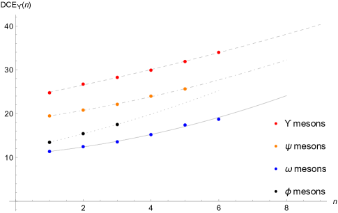
Figure 3: DCE of the isovector meson families as a function of the $n$ radial excitation level. The first form of DCE Regge trajectory is plotted as the dashed line, for the $\Upupsilon$ mesons; as the dot-dashed line, for the $\psi$ mesons; as the dotted line, for the $\phi$ mesons; and as the gray line for the $\omega$ mesons.

Linear Regge trajectories illustrate the proportionality between the radial excitation level of light-flavor mesons and the square of their mass spectrum. However, it does not hold necessarily, when heavy quarks constituents are taken into account. The DCE of isovector meson families can be also realized as a function of mass spectra of the isovector meson resonances. In this way, the second type of DCE Regge trajectories regard the experimentally detected mass spectra of the $\Upupsilon$, $\psi$, $\omega$, and $\phi$ meson $S$-wave resonances pdg . In fact, having the DCE of all states in the four isovector meson families in Tables 5 – 8, we can also plot the DCE as a function of the mass of each resonance, available in Tables 1 – 4. The results are shown in Figs. 4 – 7, respectively, whose interpolation method generates the second type of DCE Regge trajectories in Eqs. (23a) – (23d). These equations are the second type of DCE Regge trajectories, respectively, for the $\Upupsilon$, $\psi$, $\omega$, and $\phi$ isovector meson families.

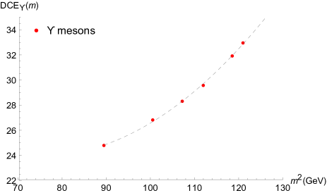
Figure 4: DCE of the $\Upupsilon$ meson family, for $n=1,\ldots,6$ (respectively corresponding to the $\Upupsilon(1S)$, $\Upupsilon(2S)$, $\Upupsilon(3S)$, $\Upupsilon(4S)=\Upupsilon(10580)$, $\Upupsilon(10860)$ and $\Upupsilon(11020)$ $S$-wave resonances in PDG pdg ) with respect to their squared mass. The DCE Regge trajectory is represented by the interpolating dashed line.

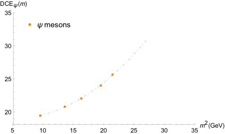
Figure 5: DCE of the $\psi$ meson family, for $n=1,\ldots,5$ (respectively corresponding to the $J/\psi(1S)$, $\psi(2S)$, $\psi(4040)$, $\psi(4415)$, and $\psi(4660)$ $S$-wave resonances in PDG pdg ) with respect to their squared mass. The DCE Regge trajectory is represented by the interpolating dot-dashed line.

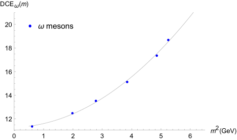
Figure 6: DCE of the $\omega$ meson family, for $n=1,\ldots,6$ (respectively corresponding to the $\omega(782)$, $\omega(1420)$, $\omega(1650)$, $\omega(1960)$, $\omega(2205)$, and $\omega(2290)$ $S$-wave resonances in PDG pdg ) with respect to their squared mass. The DCE Regge trajectory is represented by the interpolating gray line.

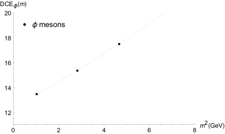
Figure 7: DCE of the $\phi$ meson family, for $n=1,\ldots,3$ (respectively corresponding to the $\phi(1020)$, $\phi(1680)$, and $\phi(2170)$ $S$-wave resonances in PDG pdg ) with respect to their squared mass. The DCE Regge trajectory is represented by the interpolating dotted line.

The second type of DCE Regge trajectories, relating the DCE of the isovector mesons to their squared mass spectra, $m^{2}$ (GeV²), respectively for the $\Upupsilon$, $\psi$, $\omega$, and $\phi$ meson families, read

$$\!\!\!\!\!\!\!\!\!\!\!\!\!\!\!\!\!\!{\color[rgb]{0,0,0}_{\Upupsilon}(m)}\! \!=\! {\color[rgb]{0,0,0}4.242\times 10^{-3}m^{4}\!-\!0.637m^{2}\!+\!47.892},$$ (23a)

$$\!\!\!\!\!\!\!\!\!\!\!\!\!\!\!\!\!\!{\color[rgb]{0,0,0}_{\psi}(m)}\! \!=\! {\color[rgb]{0,0,0}2.487\times 10^{-2}m^{4}0.260m^{2}+19.688},$$ (23b)

$$\!\!\!\!\!\!\!\!\!\!\!\!\!\!\!\!\!\!{\color[rgb]{0,0,0}_{\omega}(m)}\! \!=\! {\color[rgb]{0,0,0}0.249m^{4}+0.073m^{2}+11.273},$$ (23c)

$$\!\!\!\!\!\!\!\!\!\!\!\!\!\!\!\!\!\!{\color[rgb]{0,0,0}_{\phi}(m)}\! \!=\! {\color[rgb]{0,0,0}2.328\times 10^{-2}m^{4}\!+\!0.981m^{2}\!+\!12.435},$$ (23d)

within $1\%$ ($\Upupsilon$ and $\psi$), $1.3\%$ ($\omega$), and $0.1\%$ ($\phi$) root-mean-square deviation (RMSD).

Eqs. (22a) – (22d) and (23a) – (23d), pairwise respectively, carry the core of properties of the isovector meson families. Besides, from Eqs. (22a) – (22d) one can promptly infer the DCE of elements in each family for higher values of the $n$ excitation level of $S$-wave resonances. Subsequently, with the DCE in hands for each $n$ excitation level, one can substitute it on the left-hand side of Eqs. (23a) – (23d) and solve them, deriving the mass of each isovector meson resonance corresponding to a higher $n$ excitation level. In this way, the mass spectrum of new elements in each isovector meson family can be obtained. Besides, this method is based solely on the experimental mass spectra of the isovector meson families, which is a more realistic technique – in the sense that it uses the experimental mass spectra of isovector families – when compared to pure AdS/QCD predictions. Here we use the stress-energy tensor of AdS/QCD to compute the DCE according to (15) – (18), however Eqs. (23a) – (23d) are obtained by interpolation of the experimental mass spectra of the isovector meson families, also shown in Figs. 4 – 7.

Let us begin the analysis with the $\Upupsilon$ meson family. We want to determine the mass of the $\Upupsilon(7S)$ element in this meson family, corresponding to the $n=7$ resonance. When putting $n=7$ back into Eq. (22a), the DCE amounts to 35.961 nat. Afterwards, using this value of DCE into the left hand side of Eq. (23a), one can obtain the algebraic solution for the $m$ variable, yielding the mass of the $\Upupsilon(7S)$ resonance to be $m_{\Upupsilon(7S)}=11.328$ GeV. Now, accomplishing the same technique to the $n=8$ excitation level in Eq. (22a), the DCE underlying the $\Upupsilon(8S)$ resonance reads 38.099 nat. Subsequently working out Eq. (23a) for this value of the DCE implies the $\Upupsilon(8S)$ resonance mass to assume the value $m_{\Upupsilon(8S)}=11.527$ GeV. Analogously, the $n=9$ excitation level can be now implemented into Eq. (22a), implying the DCE of the $\Upupsilon(9S)$ resonance to be equal to 40.322 nat. When Eq. (23a) is then resolved, using this value of DCE, the $\Upupsilon(9S)$ resonance mass $m_{\Upupsilon(9S)}=11.715$ GeV is acquired. These results are compiled in Table 9.

$n$	State	$M_{\scalebox{0.67}{{Experimental}}}$ (MeV)	$M_{\scalebox{0.67}{{Theory}}}$ (MeV)
1	$\Upupsilon(1S)\;$	$9460.30\pm 0.26$	9438.51
2	$\Upupsilon(2S)\;$	$10023.26\pm 0.32$	9923.32
3	$\Upupsilon(3S)\;$	$10355\pm 0.5$	10277.2
4	$\Upupsilon(4S)\!=\!\Upupsilon(10580)\;$	$10579.4\pm 1.2$	10558.6
5	$\Upupsilon(10860)\;$	$10889.9^{+3.2}_{-2.6}$	10793.5
6	$\Upupsilon(11020)\;$	$11000\pm 4$	10995.7
7*	$\Upupsilon(7S)\;$	—–	11328.1⋆
8*	$\Upupsilon(8S)\;$	—–	11527.5⋆
9*	$\Upupsilon(9S)\;$	—–	11715.2⋆

Table 9: Table 1 completed with the higher $n$ resonances (with an asterisk) of the $\Upupsilon$ meson family. The extrapolated masses for $n=7,8,9$ in the fourth column indicated with a “ ^⋆ ” specify that they are result of the concomitant use of DCE Regge trajectories (22a, 23a), interpolating the experimental masses of $\Upupsilon$ mesons from $n=1,\ldots,6$.

Now, let us use the DCE Regge trajectories (22b, 23b) for scrutinizing the $\psi$ meson family. Firstly, we want to determine the mass of the $\psi(6S)$ meson resonance, that corresponds to the $n=6$ radial excitation level. Putting $n=6$ back into Eq. (22b) implies that the DCE is equal to 27.680 nat. Therefore, by replacing it in the left-hand side of Eq. (23b), one can solve the algebraic equation for the variable $m$. It yields the mass of the $\psi(6S)$ meson resonance to be equal to $m_{\psi(6S)}=4889.5$ MeV. Carrying out the same protocol for the $n=7$ excitation level, using the DCE Regge trajectory (22b) implies that the DCE of the $\psi(7S)$ resonance is equivalent to 29.864 nat. Hence when solving Eq. (23b), once this last value of DCE is substituted into its left-hand side, the mass of the $\psi(7S)$ meson resonance reads $m_{\psi(7S)}=5111.4$ MeV. In the same way, now utilizing the $n=8$ excitation level into Eq. (22b) yields the DCE of the $\psi(8S)$ resonance to be equal to 32.228 nat. In this case, the DCE Regge trajectory (23b) can be solved for this value, implying that the mass of the $\psi(8S)$ meson is given by $m_{\psi(8S)}=5318.7$ MeV. These results are illustrated in Table 10.

$n$	State	$M_{\scalebox{0.67}{{Experimental}}}$ (MeV)	$M_{\scalebox{0.67}{{Theory}}}$ (MeV)
1	$J/\psi(1S)\;$	$3096.900\pm 0.006$	3077.09
2	$\psi(2S)\;$	$3686.10\pm 0.06$	3689.62
3	$\psi(4040)\;$	$4039\pm 1$	4137.5
4	$\psi(4415)\;$	$4421\pm 4$	4499.4
5	$\psi(4660)\;$	$4633\pm 7$	4806.3
6*	$\psi(6S)\;$	——	4889.5⋆
7*	$\psi(7S)\;$	——	5111.4⋆
8*	$\psi(8S)\;$	——	5318.7⋆

Table 10: Table 2 completed with the higher $n$ resonances (with an asterisk) of the $\psi$ meson family. The extrapolated masses for $n=6,7,8$ in the fourth column indicated with a “ ^⋆ ” specify that they are result of the concomitant use of DCE Regge trajectories (22b, 23b), interpolating the experimental masses of $\psi$ mesons from $n=1,\ldots,5$.

In Table 10 the $\psi(4660)$ ($n=5$) resonance has a theoretically-predicted mass that is slightly higher than the mass obtained for the $\psi(6S)$ ($n=6$) resonance. The point here is that up to the $\psi(4660)$ state, the masses in the fourth column of Table 10 were derived using exclusively AdS/QCD, whereas the masses of the $\psi(6S)$, $\psi(7S)$, and $\psi(8S)$ resonances were here derived using interpolation of experimental values of the masses, namely, the third column of Table 10. Hence the monotonic profile of the masses is satisfied, since one must read in Table 10 the experimental masses of the $J/\psi(1S)$, $\psi(2S)$, $\psi(4040)$, $\psi(4415)$, $\psi(4660)$ states and, subsequently, the masses of the $\psi(6S)$, $\psi(7S)$, and $\psi(8S)$ resonances in the fourth column.

The $\omega$ isovector meson family can be analyzed, using the same approach. The $\omega(7S)$ meson resonance can have its mass derived by considering the excitation level $n=7$ in Eq. (22c), yielding the DCE equals 21.478 nat. Next, replacing it in the left hand side of Eq. (23c), and posteriorly solving for the $m$ variable implies that the $\omega(7S)$ resonance mass equals $m_{\omega(7S)}=2499.7$ MeV. Therefore accomplishing the same approach to the $n=8$ excitation level yields the DCE of the $\omega(8S)$ wave resonance to be equal to 24.087 nat, when employing the DCE Regge trajectory (22c). Subsequently resolving Eq. (23c) $m_{\omega(8S)}=2649.3$ MeV. Similarly, the $n=9$ excitation level can now be used in Eq. (22a). The DCE of the $\omega(9S)$ resonance equals 26.960 nat, using the Regge trajectory (22c). Then solving Eq. (23c) for this value, the mass of the $\omega(9S)$ meson resonance reads $m_{\omega(9S)}=2789.5$ MeV. These outcomes are shown in Table 11.

$n$	State	$M_{\scalebox{0.67}{{Experimental}}}$ (MeV)	$M_{\scalebox{0.67}{{Theory}}}$ (MeV)
1	$\omega(782)\;$	$782.65\pm 0.12$	981.43
2	$\omega(1420)\;$	$1410\pm 60$	1374
3	$\omega(1650)\;$	$1670\pm 30$	1674
4	$\omega(1960)\;$	$1960\pm 25$	1967
5	$\omega(2205)\;$	$2205\pm 30$	2149
6	$\omega(2290)\;$	$2290\pm 20$	2499.7
7*	$\omega(7S)\;$	——	2358.4⋆
8*	$\omega(8S)\;$	——	2649.3⋆
9*	$\omega(9S)\;$	——	2789.5⋆

Table 11: Table 3 completed with the higher $n$ resonances (with an asterisk) of the $\omega$ meson family. The extrapolated masses for $n=7,8,9$ in the fourth column indicated with a “ ^⋆ ” specify that they are result of the concomitant use of DCE Regge trajectories (22c, 23c), interpolating the experimental masses of $\omega$ mesons from $n=1,\ldots,6$.

The state $\omega(2330)$ with $I^{G}=0^{-}$ and $J^{PC}=1^{--}$ quantum numbers, reported in PDG 2020 pdg , has mass $2330\pm 30$ MeV and may be immediately identified to the $\omega(7S)$ isovector meson resonance. Also, the state $X(2632)$ with mass $2635.2$ MeV might be matched with the $\omega(8S)$ isovector meson resonance.

Finally, the $\phi$ isovector meson family can be studied by this method. The $\phi(4S)$ resonance corresponds to the $n=4$ excitation level. When putting $n=4$ back into Eq. (22d), the value 19.870 nat of the DCE is derived. Hence, replacing it into Eq. (23d), the $\phi(4S)$ resonance mass reads $m_{\phi(4S)}=2560.6$ MeV. For $n=5$, the DCE of the $\phi(5S)$ resonance is 22.441 nat, when the DCE Regge trajectory (22d) is employed. Therefore Eq. (23d) can be solved for it, yielding the $\phi(5S)$ resonance mass $m_{\phi(5S)}=2913.3$ MeV. Analogously, the $n=6$ excitation level in Eq. (22d) yields the DCE of the $\phi(6S)$ resonance equals 25.230 nat. Subsequently resolving Eq. (23d) for it, the $\phi(6S)$ resonance mass $m_{\phi(6S)}=3232.4$ MeV is acquired.

$n$	State	$M_{\scalebox{0.67}{{Experimental}}}$ (MeV)	$M_{\scalebox{0.67}{{Theory}}}$ (MeV)
1	$\phi(1020)\;$	$1019.461\pm 0.016$	1139.43
2	$\phi(1680)\;$	$1680\pm 20$	1583
3	$\phi(2170)\;$	$2160\pm 80$	2204
4*	$\phi(4S)\;$	——	2560.6⋆
5*	$\phi(5S)\;$	——	2913.3⋆
6*	$\phi(6S)\;$	——	3232.4⋆

Table 12: Table 4 completed with the higher $n$ resonances (with an asterisk) of the $\omega$ meson family. The extrapolated masses for $n=4,5,6$ in the fourth column indicated with a “ ^⋆ ” specify that they are result of the concomitant use of DCE Regge trajectories (22d, 23d), interpolating the experimental masses of $\phi$ mesons from $n=1,\ldots,3$.

The $\phi(6S)$ isovector meson state, whose mass is predicted to be 2913.3 MeV, might correspond to the $X(2350)$ element with experimental mass $3250\pm 28$ MeV.

IV Concluding remarks and perspectives

DCE Regge trajectories represent a successful approach to mass spectroscopy, in approaches of AdS/QCD. Here the four isovector meson families were scrutinized in this setup. Their underlying information entropy content played an important role in deriving the mass spectra of the next generation of isovector meson resonances, with a higher excitation level. To accomplish it, a shift of the quadratic dilaton (4) was used. One of the advantages of using DCE-based techniques is that the computational apparatus is simple when compared to other phenomenological approaches of AdS/QCD, including the lattice one. Another purpose of the DCE approach for isovector mesons is the interpolation of their experimental mass spectra of already detected states in PDG pdg , to derive the mass spectra of the next generation of isovector meson resonances. This is implemented by the concomitant analysis of the DCE Regge trajectories Eqs. (22a) – (22d) and (23a) – (23d), pairwise respectively to the $\Upupsilon$, the $\psi$, the $\omega$, and the $\phi$ isovector meson families. As the DCE is equivalent to the information chaoticity carried by a message, one can additionally interpret the isovector meson families as byproducts of experimental multiparticle production processes. In high-energy collisions encompassing quarks and gluons, chaos in QCD gauge dynamics may set in, and only particles in final states can be measured. The chaotic profile of collisions that produce isovector meson excitations can be then quantified by the loss of information at the end of the collision processes. This quantitative aspect was here shown to be encompassed by the DCE, providing experimental determination by the derived mass spectra of isovector meson states with higher excitation numbers.

Another important feature of this method is the configurational stability of the isovector meson resonances. Tables 5 – 8 respectively display the DCE of the $\Upupsilon$, the $\psi$, the $\omega$, and the $\phi$ isovector meson families. Besides, from the paragraph that precedes Table 10 up to the end of Sec. III, the values of the DCE of higher excitation level resonances are shown monotonically to increase as a function of their excitation level. This implies a configurational instability for higher excitation level resonances, irrespectively of the isovector meson family. It also corroborates the fact that lower excitation level resonances have been already detected in experiments pdg , as they are more dominant for the higher excitation level ones. Equivalently, given any fixed family among the $\Upupsilon$, the $\psi$, the $\omega$, and the $\phi$ isovector ones, the less massive the meson state, the less unstable they are, under the prism of DCE tools. The extrapolation of the mass spectra of isovector meson higher excitations can be formally implemented for an arbitrary excitation number $n$ with good accuracy. However, Tables 9 – 12 consider three excitation numbers beyond the experimental data, in each one of the four isovector meson families. Beyond that, further states are not explored, since they are configurationally very unstable, with high values of DCE. As such, they are unlikely to be experimentally detected, at least with proposed experiments that have been currently run.

AdS/QCD-based models that report quarkonia states were investigated in Ref. Braga:2015jca , whose DCE was computed in Ref. Braga:2017fsb , using the standard quadratic soft wall dilaton. This has been also emulated to the finite temperature and density scenario Braga:2016wkm ; Braga:2017oqw . In heavy-ions collisions that produce the quark-gluon plasma (QGP), quarkonia are originated also percolating into the QGP and, therefore, dissociating as an effect of the hot temperature. The next step of our studies consists of extending this model with the shifted dilaton potential (4). In this way, some thermal features of mesons, whose constituents are heavy quarks, can be investigated, for example, when dissociated in QGP. Also, decay constants can be studied in finite temperature models. As a preliminary study of the DCE underlying the QGP was already studied in Ref. daSilva:2017jay , one can also investigate the $\Upupsilon$ mesons suppression in heavy-ion collisions. As the $\Upupsilon$ mesons binding energy is large when compared to the one of $\psi$ resonances, the dissociation energy of $\Upupsilon$ mesons in the QGP is also expected to be higher Benzahra:1999iv . The absorption of $\Upupsilon$ and $\psi$ resonances in the hadronic matter then also consists of relevant directions of future investigations.

Acknowledgments:

RdR is grateful to FAPESP (Grants No. 2017/18897-8 and No. 2021/01089-1) and the National Council for Scientific and Technological Development – CNPq (Grants No. 303390/2019-0 and No. 406134/2018-9), for partial financial support.

References

- (1) C. E. Shannon, Bell Syst. Tech. J. 27 (1948) 379.
- (2) A. E. Bernardini and R. da Rocha, Phys. Lett. B 762 (2016) 107 [arXiv:1605.00294 [hep-th]].
- (3) M. Gleiser, M. Stephens and D. Sowinski, Phys. Rev. D 97 (2018) 096007 [arXiv:1803.08550 [hep-th]].
- (4) M. Gleiser and N. Stamatopoulos, Phys. Lett. B 713 (2012) 304 [arXiv:1111.5597 [hep-th]].
- (5) M. Gleiser and N. Stamatopoulos, Phys. Rev. D 86 (2012) 045004 [arXiv:1205.3061 [hep-th]].
- (6) G. Karapetyan, Phys. Lett. B 781 (2018) 201 [arXiv:1802.09105 [nucl-th]].
- (7) G. Karapetyan, Phys. Lett. B 786 (2018) 418 [arXiv:1807.04540 [nucl-th]].
- (8) A. E. Bernardini and R. da Rocha, Phys. Rev. D 98 (2018) 126011 [arXiv:1809.10055 [hep-th]].
- (9) L. F. Ferreira and R. da Rocha, Phys. Rev. D 99 (2019) 086001 [arXiv:1902.04534 [hep-th]].
- (10) R. da Rocha, Phys. Lett. B 814 (2021) 136112 [arXiv:2101.03602 [hep-th]].
- (11) L. F. Ferreira and R. da Rocha, Phys. Rev. D 101 (2020) 106002 [arXiv:1907.11809 [hep-th]].
- (12) C. W. Ma and Y. G. Ma, Prog. Part. Nucl. Phys. 99 (2018) 120 [arXiv:1801.02192 [nucl-th]].
- (13) G. Karapetyan, Eur. Phys. J. Plus 136 (2021) 122 [arXiv:2003.08994 [hep-ph]].
- (14) N. Barbosa-Cendejas, R. Cartas-Fuentevilla, A. Herrera-Aguilar, R. R. Mora-Luna and R. da Rocha, Phys. Lett. B 782 (2018) 607 [arXiv:1805.04485 [hep-th]].
- (15) A. E. Bernardini, N. R. F. Braga and R. da Rocha, Phys. Lett. B 765 (2017) 81 [arXiv:1609.01258 [hep-th]].
- (16) N. R. F. Braga and R. da Rocha, Phys. Lett. B 776 (2018) 78 [arXiv:1710.07383 [hep-th]].
- (17) G. Karapetyan, EPL 117 (2017) 18001 [arXiv:1612.09564 [hep-ph]].
- (18) G. Karapetyan, EPL 118 (2017) 38001 [arXiv:1705.10617 [hep-ph]].
- (19) G. Karapetyan, EPL 129 (2020) 18002 [arXiv:1912.10071 [hep-ph]].
- (20) G. Karapetyan, EPL 125 (2019) 58001 [arXiv:1901.05349 [hep-ph]].
- (21) N. R. F. Braga, L. F. Ferreira and R. da Rocha, Phys. Lett. B 787 (2018) 16 [arXiv:1808.10499 [hep-ph]].
- (22) N. R. Braga and R. da Mata, Phys. Rev. D 101 (2020) 105016 [arXiv:2002.09413 [hep-th]].
- (23) N. R. F. Braga, R. da Mata, Phys. Lett. B 811 (2018) 135918 [arXiv:2008.10457 [hep-th]].
- (24) P. Colangelo and F. Loparco, Phys. Lett. B 788 (2019) 500 [arXiv:1811.05272 [hep-ph]].
- (25) L. F. Ferreira and R. da Rocha, Phys. Rev. D 101 (2020) 106002 [arXiv:2004.04551 [hep-th]].
- (26) D. Marinho Rodrigues and R. da Rocha, Phys. Lett. B 811 (2020) 135943 [arXiv:2009.01890 [hep-th]].
- (27) P. A. Zyla et al. (Particle Data Group), Prog. Theor. Exp. Phys. 2020 (2020) 083C01.
- (28) R. A. C. Correa and R. da Rocha, Eur. Phys. J. C 75 (2015) 522 [arXiv:1502.02283 [hep-th].
- (29) R. A. C. Correa, D. M. Dantas, C. A. S. Almeida and R. da Rocha, Phys. Lett. B 755 (2016) 358 [arXiv:1601.00076 [hep-th]].
- (30) W. T. Cruz, D. M. Dantas, R. V. Maluf and C. A. S. Almeida, Annalen Phys. 531 (2019) 1970035 [1810.03991 [gr-qc]].
- (31) C. O. Lee, Phys. Lett. B 800 (2020) 135030 [arXiv:1908.06074 [hep-th]].
- (32) D. Bazeia and E. I. B. Rodrigues, Phys. Lett. A 392 (2021) 127170.
- (33) D. Bazeia, D. C. Moreira and E. I. B. Rodrigues, J. Magn. Magn. Mater. 475 (2019) 734.
- (34) A. Alves, A. G. Dias, R. da Silva, Physica 420 (2015) 1 [arXiv:1408.0827 [hep-ph]].
- (35) A. Alves, A. G. Dias, R. da Silva, Nucl. Phys. B 959 (2020) 115137 [arXiv:2004.08407 [hep-ph]].
- (36) M. Gleiser and D. Sowinski, Phys. Rev. D 98 (2018) 056026 [arXiv:1807.07588 [hep-th]].
- (37) N. R. Braga, Phys. Lett. B 797 (2019) 134919 [arXiv:1907.05756 [hep-th]].
- (38) N. R. F. Braga and O. C. Junqueira, Phys. Lett. B 814 (2021) 136082 [arXiv:2010.00714 [hep-th]].
- (39) R. Casadio and R. da Rocha, Phys. Lett. B 763 (2016) 434 [arXiv:1610.01572 [hep-th]].
- (40) A. Fernandes-Silva, A. J. Ferreira-Martins and R. da Rocha, Phys. Lett. B 791 (2019) 323 [arXiv:1901.07492 [hep-th]].
- (41) A. E. Bernardini and R. da Rocha, Phys. Lett. B 796 (2019) 107 [arXiv:1908.04095 [gr-qc]].
- (42) C. O. Lee, Phys. Lett. B 790 (2019) 197 [arXiv:1812.00343 [gr-qc]].
- (43) P. Thakur, M. Gleiser, A. Kumar and R. Gupta, Phys. Lett. A 384 (2020) 126461 [arXiv:2011.06926 [nlin.PS]].
- (44) C. Amsler et al., Eur. Phys. J. C 33 (2004) 23.
- (45) Y. A. Simonov, Phys. Lett. B 226 (1989) 151.
- (46) A. M. Badalian and B. L. G. Bakker, Phys. Rev. D 93 (2016) 074034 [arXiv:1603.04725 [hep-ph]].
- (47) T. Frederico, K. S. F. F. Guimarães, O. Lourenço, W. de Paula, I. Bediaga and A. C. dos Reis, Few Body Syst. 55 (2014) 441 [arXiv:1402.6975 [hep-ph]].
- (48) W. de Paula and T. Frederico, Phys. Lett. B 693 (2010) 287 [arXiv:0908.4282 [hep-ph]].
- (49) A. Karch, E. Katz, D. T. Son and M. A. Stephanov, Phys. Rev. D 74 (2006) 015005 [hep-ph/0602229].
- (50) C. Csaki, M. Reece, JHEP 05 (2007) 062 [arXiv:hep-ph/0608266].
- (51) T. Branz, T. Gutsche, V. E. Lyubovitskij, I. Schmidt and A. Vega, Phys. Rev. D 82 (2010) 074022 [arXiv:1008.0268 [hep-ph]].
- (52) P. Colangelo, F. De Fazio, F. Giannuzzi, F. Jugeau and S. Nicotri, Phys. Rev. D 78 (2008) 055009 [arXiv:0807.1054 [hep-ph]].
- (53) M. A. Martin Contreras and A. Vega, Phys. Rev. D 102 (2020) 046007 [arXiv:2004.10286 [hep-ph]].
- (54) S. S. Afonin and I. V. Pusenkov, Phys. Rev. D 90 (2014) 094020 [arXiv:1411.2390 [hep-ph]].
- (55) J. K. Chen, Eur. Phys. J. C 78 (2018) 648.
- (56) B. Fuks, K. Hagiwara, K. Ma and Y. J. Zheng, [arXiv:2102.11281 [hep-ph]].
- (57) N. R. F. Braga, M. A. Martin Contreras, S. Diles, Phys. Lett. B 763 (2016) 203 [arXiv:1507.04708 [hep-th]].
- (58) E. Witten, Adv. Theor. Math. Phys. 2 (1998) 253 [hep-th/9802150].
- (59) D. Besson et al. [CLEO], Phys. Rev. Lett. 54 (1985) 381.
- (60) Y. H. Chen, M. Cleven, J. T. Daub, F. K. Guo, C. Hanhart, B. Kubis, U. G. Meißner and B. S. Zou, Phys. Rev. D 95 (2017) 034022 [arXiv:1611.00913 [hep-ph]].
- (61) B. Aubert et al. [BaBar], Phys. Rev. D 72 (2005) 032005 [arXiv:hep-ex/0405025 [hep-ex]].
- (62) E. Braaten and D. Kang, Phys. Rev. D 88 (2013) 014028 [arXiv:1305.5564 [hep-ph]].
- (63) N. R. F. Braga, M. A. Martin Contreras, S. Diles, Eur. Phys. J. C 76 (2016) 598 [arXiv:1604.08296 [hep-ph]].
- (64) N. R. F. Braga and L. F. Ferreira, Phys. Lett. B 773, 313 (2017).
- (65) N. R. F. Braga, L. F. Ferreira and A. Vega, Phys. Lett. B 774 (2017) 476 [arXiv:1709.05326 [hep-ph]].
- (66) A. Goncalves and R. da Rocha, Phys. Lett. B 774 (2017) 98 [arXiv:1706.01482 [hep-ph]].
- (67) S. C. Benzahra, Phys. Rev. C 61 (2000) 064906 [arXiv:hep-ph/9904231 [hep-ph]].