Atomic Carbon [CI]$(^{3}P_{1}-^{3}P_{0})$ Mapping of the Nearby Galaxy M83

Abstract

Atomic carbon (CI) has been proposed to be a global tracer of the molecular gas as a substitute for CO, however, its utility remains unproven. To evaluate the suitability of CI as the tracer, we performed [CI]$(^{3}P_{1}-^{3}P_{0})$ (hereinafter [CI](1–0)) mapping observations of the northern part of the nearby spiral galaxy M83 with the ASTE telescope and compared the distributions of [CI](1–0) with CO lines (CO(1–0), CO(3–2), and CO13(1–0)), HI, and infrared (IR) emission (70, 160, and 250$~{}\mu$m). The [CI](1–0) distribution in the central region is similar to that of the CO lines, whereas [CI](1–0) in the arm region is distributed outside the CO. We examined the dust temperature, $T_{\rm dust}$, and dust mass surface density, $\Sigma_{\rm dust}$, by fitting the IR continuum-spectrum distribution with a single temperature modified blackbody. The distribution of $\Sigma_{\rm dust}$ shows a much better consistency with the integrated intensity of CO(1–0) than with that of [CI](1–0), indicating that CO(1–0) is a good tracer of the cold molecular gas. The spatial distribution of the [CI] excitation temperature, $T_{\rm ex}$, was examined using the intensity ratio of the two [CI] transitions. An appropriate $T_{\rm ex}$ at the central, bar, arm, and inter-arm regions yields a constant [C]/[H₂] abundance ratio of $\sim 7\times 10^{-5}$ within a range of 0.1 dex in all regions. We successfully detected weak [CI](1–0) emission, even in the inter-arm region, in addition to the central, arm, and bar regions, using spectral stacking analysis. The stacked intensity of [CI](1–0) is found to be strongly correlated with $T_{\rm dust}$. Our results indicate that the atomic carbon is a photodissociation product of CO, and consequently, compared to CO(1–0), [CI](1–0) is less reliable in tracing the bulk of ”cold” molecular gas in the galactic disk.

1 Introduction

Molecular hydrogen (H₂) is a major constituent of the interstellar medium in galaxies. However, direct detection of cold H₂ is difficult because H₂ lacks a permanent dipole moment due to its symmetric structure. Alternatively, the amount of H₂ has been indirectly estimated by observing CO, which is the second most abundant species in molecular clouds. CO has a weak permanent dipole moment and a ground rotational transition with a low excitation energy of $\sim 5.5$ K. Owing to this low energy and critical density ($n_{\rm cr}\sim 10^{3}$ cm^-3, however, $n_{\rm cr}$ is further reduced by radiative trapping due to its large optical depth), CO is easily excited even in cold molecular clouds. Meanwhile, the large optical depth makes it difficult to estimate the molecular gas mass. Furthermore, in a low-metal environment, the CO lines are not necessarily suitable for tracing the amount of molecular gas because of CO depletion that is caused by the lack of heavy elements and by the photo-dissociation due to the interstellar radiation field as a result of poor (self)shielding (e.g., [Israel (1997)], [Leroy et al. (2007)]).

The forbidden fine-structure transition lines of atomic carbon, namely, [CI]$(^{3}P_{1}-^{3}P_{0})$ and [CI]$(^{3}P_{2}-^{3}P_{1})$, hereinafter [CI](1–0) and [CI](2–1), respectively, are optically thin in most cases (e.g., [Ikeda et al. (2002)]); further, they have excitation energies of 23.6 K and 62.5 K, respectively, and the critical density of [CI](1–0) ($n_{\rm cr}\approx 10^{3}$ cm^-3) is similar to that of CO(1–0). In addition, although the classical photodissociation region (PDR) models ([Tielens & Hollenbach (1985)], [Hollenbach et al. (1991)]) expect the atomic carbon to exist predominantly in the thin layer near the surface of a homogeneous static molecular cloud that is exposed to UV radiation, [CI](1–0) mapping observations of galactic molecular clouds have shown that the distribution of [CI](1–0) is similar to that of low-$J$ CO (and CO13) lines (e.g.,[Tauber et al. (1995)], [Ikeda et al. (2002)], [Shimajiri et al. (2013)]). The co-existence of [CI](1–0) with CO can be explained by introducing density inhomogeneity in the densities of molecular clouds in the classical PDR, because it allows the external radiation to penetrate deeply into the cloud (e.g., [Spaans (1996)]). Recent refined simulations such as those considering the turbulence of the clouds (Glover et al., 2015) or the influence of cosmic rays (e.g., Bisbas et al. (2015), Papadopoulos, et al. (2018)) have confirmed the widespread distribution of [CI](1–0) in the clouds. The results of both these observations and theories have encouraged the understanding that [CI] could be a molecular gas tracer alternative to low-$J$ CO.

Recently, owing to the availability of the Atacama Large Millimeter/submillimeter Array (ALMA) and Hershel/SPIRE, the relation between [CI] and CO for extra-galaxies has been actively surveyed to confirm the utility of [CI] as a molecular gas tracer [e.g., Israel et al. (2015), Jiao et al. (2017), and Jiao et al. (2019) for local and (ultra)luminous infrared galaxies ((U)LIRGs); Valentino et al. (2018) for high-redshift galaxies]. Jiao et al. (2017) and Jiao et al. (2019) have demonstrated a strong (nearly linear) relation between [CI] and CO(1–0) line luminosities for (U)LIRGs and local galaxies, and concluded that [CI](1–0) is likely a good molecular gas mass tracer. In contrast, Israel et al. (2015) argued that [CI](1–0) may trace dense clouds rather than a diffuse gas, and consequently, it is not a good tracer of the bulk of molecular gas. Moreover, through observations of the individual galaxies, a careful treatment for using [CI](1–0) as an alternative molecular gas tracer to CO is cautioned because of the spatial variance of the [CI]–CO relation (e.g., Salak et al. (2019), Saito et al. (2020)). Thus, whether [CI] can be a H₂ tracer as a substitute for CO is under debate. Notably, the investigations of the relation between [CI](1–0) and CO have been mainly biased toward CO-bright sources, such as star-forming clouds, the centers of galaxies, and (U)LIRGs, thus far. To understand the CI–CO relation and the utility of [CI](1–0) as a molecular gas tracer, it is necessary to compare CI and CO with H₂ estimated by an independent method, independent of the brightness of CO.

Infrared (IR) dust emission, which is optically thin over most regions of normal galaxies is another tool to estimate the molecular gas surface density, $\Sigma_{\rm mol}$. Under the assumptions that dust and gas are well mixed and the gas-to-dust ratio (GDR) is fixed in the atomic and molecular phases, the dust mass surface density, $\Sigma_{\rm dust}$, measured with the IR emission can be converted to the total gas surface density, $\Sigma_{\rm gas}$, using the GDR. Then, $\Sigma_{\rm mol}$ can be obtained by subtracting the contribution of the atomic gas surface density, $\Sigma_{\rm atom}$, based on the HI measurement from $\Sigma_{\rm gas}$. However, the determination of GDR is an unresolved issue. Considering the following equation,

$$\Sigma_{\rm gas} = \textrm{GDR}~{}\Sigma_{\rm dust}$$ (1)

$$= \Sigma_{\rm atom}+\alpha_{\rm\atom{CO}{}{}}I_{\rm\atom{CO}{}{}},$$

where $\alpha_{\rm\atom{CO}{}{}}$ is the CO-to-H₂ conversion factor and $I_{\rm\atom{CO}{}{}}$ is the measured CO integrated intensity, Leroy et al. (2011) proposed a technique to simultaneously measure the GDR and $\alpha_{\rm\atom{CO}{}{}}$ under the assumption that the GDR is constant over a region of the galaxy. Applying this technique to resolved galaxies allows us to compare [CI] and CO with the dust-based $\Sigma_{\rm mol}$ for each galactic structure.

M83 is an ideal target to investigate the [CI]–CO relation for the galactic structures, because it is one of the nearest (4.5 Mpc, Thim et al. (2003)) spiral galaxies that is nearly face-on (inclination=24D; Comte (1981)) and hosts prominent galactic structures (a bar and spiral arms). Moreover, multi-wavelength images for HI, CO, IR, and optical observations can be acquired from the archives. The basic parameters of M83 adopted in this paper are summarized in Table 1.

Parameters of M83 Parameter Value $\alpha_{\rm J2000.0}$^a 13h37m00s.48 $\delta_{\rm J2000.0}$^a -29D51’56”.48 Distance^b 4.5 Mpc Position angle^c 225D Inclination angle^c 24D $R_{25}$^d 644 Systemic velocity (LSR)^e $514\pm 5$ km s^-1 Linear scale (Beam size $=18\farcs 9$) $\sim 412$ pc

• Sukumar et al. (1987)

• Thim et al. (2003)

• Comte (1981)

• de Vaucouleurs et al. (1991)

• Kuno et al. (2007)

2 Observations and Analyses

2.1 CI data

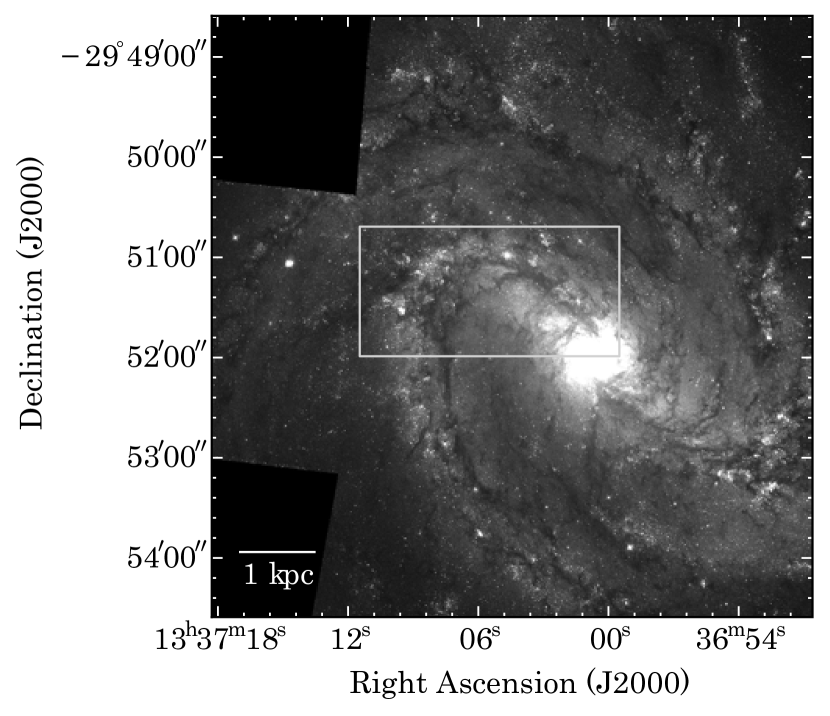
Figure 1: Observed $\timeform{150^{\prime\prime}}\times\timeform{72^{\prime\prime}}$ area (gray line) using the ASTE superposed on a V-band image of M83 retrieved from the data archive of the HST/WFC3 Early Release Science Program.

Observations of M83 in [CI](1–0) ($\nu_{\rm rest}=492.160651$ GHz) were carried out from July to August of 2017 and July 2019 using the ASTE 10-m telescope. The observations were performed in the on-the-fly (OTF) mapping mode (Sawada et al., 2008). The observed area covered a $\timeform{150^{\prime\prime}}\times\timeform{72^{\prime\prime}}$ rectangular region with PA$=\timeform{0D}$ and its center offset from the galactic center $(\alpha,\delta)_{\rm J2000.0}=$ (13h37m00s.48, -29D51’56”.48) (Sukumar et al., 1987) was ($\Delta\alpha,\Delta\delta$)=($\timeform{65^{\prime\prime}},\timeform{36^{\prime\prime}}$) so that the area could include the galactic center, the northern galactic bar, and a part of the northern spiral arm (Figure 1). The effective beam size was 189 at 492 GHz for the OTF observations, corresponding to 412 pc at a distance of 4.5 Mpc (Thim et al., 2003), which allowed us to distinguish the galactic structures, such as the bar and arm. The scan separation, perpendicular to the scan direction, was 6” and the mapping was performed in two orthogonal scan directions so that the noise temperatures in each direction were as even as possible to remove any effects of scanning noise. Two points with 10’ offset from the map center in the direction of the declination were used as the off-source positions. The pointing toward a Mira-type variable star W Hya was checked every 1–2 hr by observing CO(3–2), and the accuracy was better than 4”.

The utilized frontend was a two-sideband dual-polarization heterodyne receiver of ASTE Band 8 and the backend was an FX-type spectrometer, WHSF, with a total bandwidth of 2048 MHz. The total number of channels was 2048, with a spectral resolution of 1 MHz (0.6 km s^-1 at 492 GHz), and a velocity coverage of 1248 km s^-1. The system noise temperature at 492 GHz ranged from 500 to 2500 K. The line intensity was calibrated by the chopper wheel method, yielding an antenna temperature, $T_{\rm A}^{\ast}$, corrected for both atmospheric and antenna ohmic losses (Ulich & Haas, 1976). In this study, we used the main beam brightness temperature $T_{\rm mb}\equiv T_{\rm A}^{\ast}/\eta_{\rm mb}$, with the main beam efficiency of the antenna, $\eta_{\rm mb}=$ 0.45. The antenna temperature of 1 K corresponds to 127.2 Jy at 492 GHz. The absolute intensity and the variation in the main beam efficiency was checked by observing M 17 in [CI] and comparing the standard spectra of M 17 (White & Padman, 1991). The uncertainty of the efficiency was estimated to be better than 20%.

We used an auto-reduction system, COMING ART (Sorai et al., 2019), for data reduction, based on Nobeyama OTF Software Tools for Analysis and Reduction (NOSTAR), developed by Nobeyama Radio Observatory. The COMING ART system flagged and removed poor quality data after applying a linear baseline fitting, and then performed the basket weaving procedure to reduce the scanning effect (Emerson & Graeve, 1988). Before preparing the final [CI] cube data with 6” spacing and a velocity width of 10 km s^-1, a cubic polynomial baseline fitting was applied in the emission-free range to optimize the zero level in each spectrum. The resultant rms noise level was typically 25 mK in the $T_{\rm mb}$ scale.

2.2 CO data

We retrieved the CO12(1–0), CO13(1–0), and CO12(3–2) data from the ALMA archive (projects 2012.1.00762.S and 2015.1.01593.S, PI: Hirota), all of which contained data obtained with the 12-m, 7-m, and total power (TP) arrays. To obtain images matching with the spatial resolution of [CI], we used the data obtained with the 7-m and TP arrays for CO12(1–0) and CO13(1–0) and the TP array for CO12(3–2). We processed the data with the observatory-provided calibration scripts through CASA (McMullin et al., 2007). The calibration was carried out in CASA version 4.5.3 or 4.7.2, following the manuals provided by the observatory. After inspecting the calibrated data, we subtracted the continuum emission for each line determined at the emission-free channels. Imaging of the interferometric data was performed in tclean in CASA version 5.6.1, where visibilities in baselines longer than $\sim 12$ k$\lambda$ in the uv-plane were tapered to maximize sensitivity to the extended structures. The calibrated TP data in each line were imaged in sdimaging. Finally, we combined these data with the Feather algorithm in CASA. All of the final data were spatially smoothed to match the resolution of the [CI] data (18.9”).

2.3 HI data

To trace the atomic hydrogen gas surface density of M83, we retrieved the HI image from The H I Nearby Galaxy Survey (THINGS; Walter et al. (2008)) with the Very Large Array (VLA). We used the natural weighted maps with a resolution of $15\farcs 2\times 11\farcs 4$ and converted the integrated intensity to a surface density following Walter et al. (2008). The uncertainty of HI flux density was $\sim 5\%$ due to the flux calibration. The HI map was aligned and convolved to match the [CI](1–0) image.

2.4 Infrared data

The Very Nearby Galaxy Survey (VNGS, Bendo et al. (2012)) observed M83 using Herschel/PACS at 70 $\mu$m and 160 $\mu$m and with Herschel/SPIRE at 250 $\mu$m, 350 $\mu$m, and 500 $\mu$m. The full width at half-maximum (FWHM) of the point spread functions were 60, 120, 182, 245, and 360 for 70 $\mu$m, 160 $\mu$m, 250 $\mu$m, 350 $\mu$m, and 500 $\mu$m, respectively. The calibration uncertainties corresponding to 70 $\mu$m, 160 $\mu$m, 250 $\mu$m, 350 $\mu$m, and 500 $\mu$m, were 0.03, 0.05, 0.07, 0.07, and 0.07, respectively (Foyle et al., 2012). Using the images at each wavelength, Foyle et al. (2012) derived the dust temperature and mass surface density of M83 through the modified blackbody fitting in the IR regime on each pixel with 360 resolution. Consequently, they found that the temperature ranged from 20 to 30 K over the entire disk in both cases of a variable and constant dust emissivity index $\beta$. We, therefore, used the images at 70 $\mu$m, 160 $\mu$m, and 250 $\mu$m in this work (the peak of the blackbody curve is within the wavelengths) , obtaining the properties on an angular scale matching with the spatial resolution of [CI](1–0). The images were all aligned and convolved to the [CI] image after applying calibration and conversion to Jy/sr^-1, following Foyle et al. (2012).

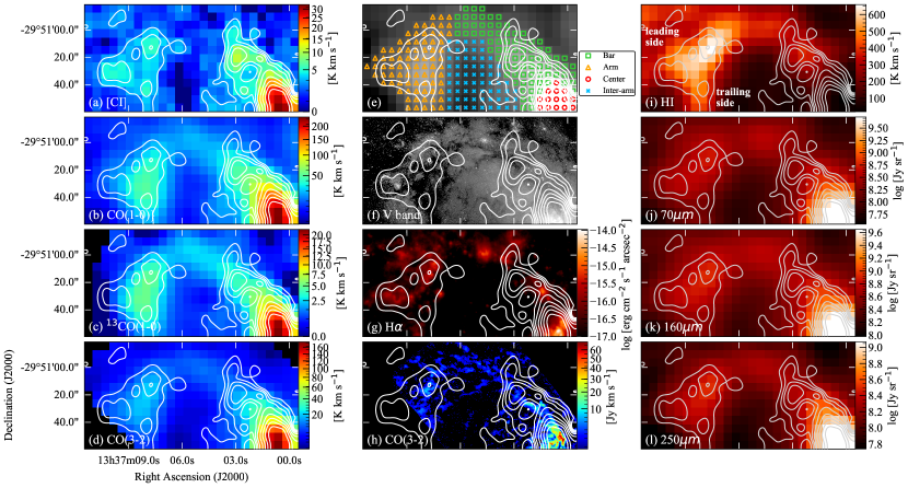
Figure 2: Integrated intensity maps of (a) [CI](1–0), (b) CO12(1–0) (c) CO13(1–0). (d) CO12(3–2). In panel (e), the regions defined as central region, barred region, arm region, and inter-arm region are denoted by circles, squares, triangles, and crosses, respectively. Panels (f), (g), and (h) are V-band, H$\alpha$, and CO12(3–2) images at their original resolutions. In panel (d), only the TP array data is used for the CO12(3–2) image, whereas the data of the 12-m, 7-m, and TP arrays are combined for the image in panel (h). Therefore, the image area is limited by the field of view of the12-m array. Panels (i), (j), (k), and (l) depict the integrated intensity map of HI and surface brightness maps at 70 $\mu$m, 160 $\mu$m, and 250 $\mu$m, respectively. Contours in all panels show the integrated intensity of [CI](1–0), corresponding to 3, 5, 7, 10, 15, 20, 25, and 30 $\sigma$, where 1$\sigma=$ 0.85 K km s^-1,

3 Results

3.1 Distribution of [CI](1–0) intensity and comparison with data corresponding to other wavelengths

Figure 2(a) shows the integrated intensity map ($I=\int T_{\rm mb}~{}dv$) of [CI](1–0), where $T_{\rm mb}$ is the main beam brightness temperature, and the contours of $I_{\rm[\atom{C}{}{}\emissiontype{I}](1-0)}$ are superposed on the remaining panels (Figure 2(b)–(l)). A maximum integrated intensity of $I_{\rm[\atom{C}{}{}\emissiontype{I}](1-0)}=32.68\pm 1.75$ K km s^-1 is found at the center, $(\alpha,\delta)_{\rm J2000.0}=$ (13h37m00s.48, -29D51’56”.48). The integrated intensity maps of CO12($J=1-0$), CO13($J=1-0$), and CO12($J=3-2$) with the same angular resolution as that of [CI](1–0) are shown in Figure 2(b)–(d). The uncertainty of the integrated intensity was calculated as $\Delta I=T_{\rm rms}\sqrt{\Delta V_{\rm int}V_{\rm ch}}$, where $T_{\rm rms}$ is the rms noise calculated over the emission-free channels, $\Delta V_{\rm int}$ is the full velocity width of the emission channels, and $V_{\rm ch}=10$ km s^-1 is the velocity width of a single channel. The uncertainties in [CI](1–0), CO12($J=1-0$),CO12($J=3-2$), and CO13($J=1-0$) were typically 0.85, 0.69, 0.16, and 0.14 K km s^-1, respectively. We defined the central region, bar region, spiral arm region, and the inter-arm region by referring to the CO(1–0) map (Figure 2(e)). A comparison of the distributions of [CI](1–0) and CO lines in Figure 2(b)–(d) reveals that both are strong in the central region and are similarly distributed in the bar region, whereas [CI](1–0) is distributed outside the CO gas in the spiral arm.

We compared the [CI](1–0) distribution with the V-band (obtained from the [CI](1–0) mapping area in Figure 1), H$\alpha$, and CO(3–2) images at their original resolutions in Figure 2(f)–(h). The continuum-subtracted H$\alpha$ image was observed by the Survey for Ionization in Neutral Gas Galaxies (SINGG, Meurer et al. (2006)) using the Cerro Tololo Inter-American Observatory (CTIO) 1.5 m telescope. The data were acquired from the NASA/IPAC Extragalactic Database. The CO(3–2) image with a high spatial resolution of $0\farcs 7$ was produced using the ALMA 12-m, 7-m, and TP arrays in the same manner as described in section 2.2. The [CI](1–0) distribution in the arm region, especially in the leading side (assuming trailing spiral arms), was in good agreement with the H$\alpha$ and CO(3–2) distributions, although the CO(3–2) image does not entirely cover the arm region due to the limitation of observing the area with the 12-m array.

Figures 2(i)–(l) compare the [CI](1–0) map with those of the integrated intensity of HI and the surface brightness of 70 $\mu$m, 160 $\mu$m, and 250 $\mu$m. The HI  emission has a hole at the central region, and the patterns of the HI and [CI](1–0) spiral arms are consistent not only on the leading side but also the trailing side. In addition, the brightness of the image at 70 $\mu$m is stronger on the leading side of the arm than on the trailing side, whereas that at 250 $\mu$m is extended throughout the arm as with CO(1–0). This is compatible with the result that CO(1–0) and 100 $\mu$m are not well correlated (Crosthwaite et al., 2002). Based on the comparison of the dust color temperatures for the 70, 160, 250, 350, and 500 $\mu$m bands with H$\alpha$, Bendo et al. (2012) argued that the dust emission at wavelengths shorter than 160 $\mu$m could be affected by the star-forming region, whereas the wavelengths longer than 250 $\mu$m could be less affected and trace cold dust. Furthermore, the fact that HI correlates better with 70 $\mu$m and H$\alpha$ than with 250 $\mu$m and that it is strong on the leading side of the arm, is consistent with the understanding that HI  is a photodissociation product (e.g., Rand et al. (1992), Hirota et al. (2018)).

3.2 [CI] – CO correlation

Figure 3: Plots of the line luminosities of (a) CO(1–0), (b) CO(3–2), and (c) CO13(1–0) against that of [CI](1–0) above 4$\sigma$. The circle, square, and triangle symbols correspond to the central region, barred region, and arm region, respectively, corresponding to those in Figure 2(e). The best-fit relation with a fixed slope of unity for all regions is shown by the gray solid line, and the best-fit relation without fixing the slope is shown by the black dashed-dotted line. The dotted lines represent 0.5 dex offset from the solid line. The (pink) dashed line in panel (a) is the best-fit relation with a fixed slope of unity for nearby galaxies (Jiao et al., 2019).

Determined Parameters and Correlation Coefficient Line Region $A$ $B$ $R_{A,B}^{2}$ $C$ $R_{C}^{2}$ CO(1–0) All $1.15\pm 0.05$ $0.09\pm 0.26$ $0.63$ $0.88\pm 0.01$ $0.69$ Center $0.65\pm 0.08$ $2.83\pm 0.45$ $0.79$ $0.92\pm 0.02$ $0.57$ CO(3–2) All $1.40\pm 0.06$ $-1.55\pm 0.30$ $0.66$ $0.60\pm 0.02$ $0.73$ Center $0.93\pm 0.12$ $1.11\pm 0.65$ $0.78$ $0.70\pm 0.02$ $0.78$ CO13(1–0) All $1.14\pm 0.05$ $-0.92\pm 0.28$ 0.58 $-0.19\pm 0.02$ 0.64 Center $0.82\pm 0.07$ $0.85\pm 0.41$ 0.88 $-0.16\pm 0.02$ 0.83

We compared the line luminosities between CO(1–0) and [CI](1–0) in a pixel-by-pixel manner, and both the lines were detected above the $4\sigma$ noise level (Figure 3(a)). The line luminosity, $L^{\prime}_{\rm line}$, in units of K km s^-1 pc² was calculated as the product of the integrated intensity, $I_{\rm line}$, and the projected pixel area, $A_{0}$, in pc², as: $L^{\prime}_{\rm line}=I_{\rm line}A_{0}$ (cf. Solomon & Vanden Bout (2005)). Although the correlation between CO(1–0) and [CI](1–0) is worse in the arm region in Figure 2 and 3, the overall distribution of both luminosities in the whole disk is correlated with each other in Figure 2. The CO(1–0)–[CI](1–0) relation was fitted by:

$$\log L^{\prime}_{\rm\atom{CO}{}{}(1-0)} = A\log L^{\prime}_{\rm[\atom{C}{}{}\emissiontype{I}](1-0)}+B~{}[{\rm K~{}km~{}s^{-1}~{}pc^{2}}],$$ (2)

$$L^{\prime}_{\rm\atom{CO}{}{}(1-0)} = 10^{B}~{}{L^{\prime}}_{\rm[\atom{C}{}{}\emissiontype{I}](1-0)}^{A},$$ (3)

using orthogonal distance regression (ODR). The coefficients $(A,B)$ were derived as $(1.15\pm 0.05,0.09\pm 0.26)$ with the coefficient of determination, $R^{2}=0.63$ (black dashed-dotted line in Figure 3(a), Table 3.2). The slope was slightly steeper than that of the relation for nearby galaxies that were observed at a scale of $\sim 1$ kpc, as shown by Jiao et al. (2019), where reportedly $(A,B)=(1.04\pm 0.02,0.74\pm 0.12)$. The steep slope is mainly caused by the relation in the arm region (triangle symbols in Figure 3), lying below the relation in the central region. The least square fit to the data only in the central region yields coefficients as $(A,B)=(0.65\pm 0.08,2.83\pm 0.45)$, wherein the observed shallow slope is in agreement with that for the central region of the nearby starburst/Seyfert galaxy NGC 1808 ($0.686\pm 0.010$, Salak et al. (2019)) and for LIRG IRAS F18293-3413 ($0.65\pm 0.01$, Saito et al. (2020)).

By fitting the relationship of the line luminosities in all regions, including the center, bar, and arm, with a fixed slope of unity using ODR, i.e.,

$$\log L^{\prime}_{\rm\atom{CO}{}{}(1-0)} = \log L^{\prime}_{\rm[\atom{C}{}{}\emissiontype{I}](1-0)}+C~{}[{\rm K~{}km~{}s^{-1}~{}pc^{2}}],$$ (4)

$$L^{\prime}_{\rm\atom{CO}{}{}(1-0)} = 10^{C}~{}L^{\prime}_{\rm[\atom{C}{}{}\emissiontype{I}](1-0)},$$ (5)

the coefficient $C=0.88\pm 0.01$ was derived with $R^{2}=0.69$. This is represented by the gray solid line in Figure 3, where the intercept $C$ corresponds to the logarithm of the luminosity ratio of CO(1–0) to [CI](1–0). The intercept of the data only in the central region, $C=0.92\pm 0.02$ with $R^{2}=0.57$, is comparable to that in nearby galaxies $(C=0.96\pm 0.01)$, as reported by Jiao et al. (2019).

Thus far, the [CI](1–0) and CO(1–0) luminosity relation in galaxies has been determined by measurements of CO-bright sources, such as the galactic centers and (U)LIRGs. The relationship in the CO-bright region in the arm of M 83 follows the main relation ($C\sim 1$), corresponding to the integrated intensity ratio, $I_{\rm[\atom{C}{}{}\emissiontype{I}]}/I_{\rm\atom{CO}{}{}(1-0)}$ [denoted by $R_{\rm[\atom{C}{}{}\emissiontype{I}]/\atom{CO}{}{}}$ $(=L^{\prime}_{\rm[\atom{C}{}{}\emissiontype{I}]}/L^{\prime}_{\rm\atom{CO}{}{}(1-0)})$], of $\sim 0.1$ (equation (5)), which is comparable to that for the central region of 30 nearby galaxies, $R_{\rm[\atom{C}{}{}\emissiontype{I}]/\atom{CO}{}{}}$  $=0.16\pm 0.08$ (Israel, 2020). However, the data from the leading side of the arm (i.e., CO-dark region) is deviated from the main relation, i.e., [CI](1–0) enhancement to CO(1–0). Ojha et al. (2001) found that $R_{\rm[\atom{C}{}{}\emissiontype{I}]/\atom{CO}{}{}}$  at the Galactic center $(\sim 0.1)$ is lower than that in the disk $(\sim 0.3-0.4)$. Even for nearby galaxies, the similar trend that $R_{\rm[\atom{C}{}{}\emissiontype{I}]/\atom{CO}{}{}}$ at the center is lower than that in the disk has also been reported by Gerin & Phillips (2000). To understand the general relation between the [CI](1–0) and CO(1–0) luminosities in galaxies, their measurements, both in the central as well disk regions, are necessary.

Figures 3(b) and (c) compare the line luminosities of CO(3–2) to [CI](1–0) and CO13(1–0) to [CI](1–0), respectively, on a pixel-by-pixel basis. The relations were fitted in the same manner as that of [CI](1–0)–CO(1–0) luminosities, and the resultant coefficients are summarized in Table 3.2. Using the central region data, nearly linear fits were obtained for the relations of [CI](1–0)–CO(3–2) and [CI](1–0)-¹³CO(1–0). The slope, $A$, for [CI](1–0)–CO(3–2) is in good agreement with that obtained by Salak et al. (2019) for the nearby galaxy NGC 1808 ($A=0.942\pm 0.014$). As with the relation for the [CI](1-0)–CO(1-0) relation, the slope, $A$, of [CI](1–0)–CO(3–2) and [CI](1–0)-CO13(1–0), calculated by using the data from all the regions, is steeper than that in the central region, as the arm region is located below the relation in the central region.

We also fitted the [CI](1–0)–CO(3–2) and [CI](1–0)-CO13(1–0) luminosities with a fixed slope of unity. The calculated intercepts, $0.70\pm 0.02$ for [CI](1–0)–CO(3–2) and $-0.19\pm 0.02$ for [CI](1–0)-CO13(1–0), were compatible with the integrated intensity ratios, $I_{\rm[\atom{C}{}{}\emissiontype{I}](1-0)}/I_{\rm\atom{CO}{}{}(3-2)}$ ($\sim 0.1-0.3$) and $I_{\rm[\atom{C}{}{}\emissiontype{I}](1-0)}/I_{\rm\atom{CO}{}{13}(1-0)}$ ($\sim 1-10$ ) for the central region of the nearby galaxy NGC 613 (Miyamoto et al., 2018). The large scatter ($\pm 0.5$ dex) in the disk region data for both relations may reflect the physical properties of the gas, e.g., kinetic temperature for [CI](1–0)–CO(3–2) relation (Ikeda et al., 1999) and optical depth for [CI](1–0)-CO13(1–0) relation (Miyamoto et al., 2018).

3.3 Dust temperature and dust mass surface density

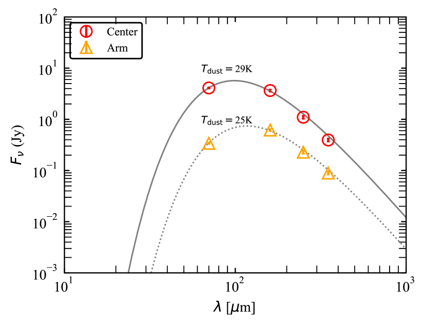
Figure 4: Plots for two examples of the initial modified blackbody fitting at 70, 160, 250, and 350 $\mu$m for pixels at the central region and arm regions, denoted by circle and triangle symbols, respectively, in Figure 5. The best-fitting is shown as a solid curve (center) and a dotted curve (arm). The best-fitting parameters obtained by using the data at 350 $\mu$m are adopted as the initial values for the modified blackbody fitting at each pixel using the data only at 70 $\mu$m, 160 $\mu$m, and 250 $\mu$m.

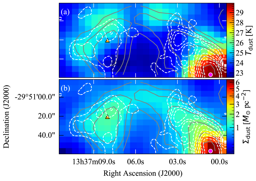
Figure 5: Spatial distribution (color) of (a) dust temperature, $T_{\rm dust}$, and (b) dust mass surface density, $\Sigma_{\rm dust}$, overlaid with the integrated intensity of [CI](1–0) (white dashed line) and CO(1–0) (gray solid line). The contours of [CI](1–0) are the same as in Figure 2 and the contours of CO(1–0) are 20, 30, 50, 100, 200, and 300 $\sigma$, where 1$\sigma=$ 0.686 K km s^-1. The circle at the center and triangle in the arm indicate the location of the pixels for which the best-fitting plots are shown in Figure 4.

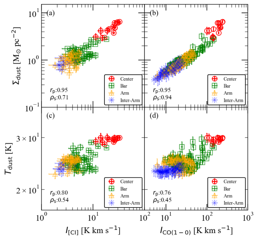
Figure 6: The correlations of $\Sigma_{\rm dust}$ to (a) $I_{\rm[\atom{C}{}{}\emissiontype{I}](1-0)}$ and (b) $I_{\rm\atom{CO}{}{}(1-0)}$, and of $T_{\rm dust}$ to (c) $I_{\rm[\atom{C}{}{}\emissiontype{I}](1-0)}$ and (d) $I_{\rm\atom{CO}{}{}(1-0)}$. The circle, square, triangle, and cross symbols indicate the central region, barred region, arm region, and inter-arm region, respectively. Pearson’s correlation coefficient ($r_{\rm p}$) and Spearman’s rank correlation coefficient ($\rho_{\rm s}$) are labeled in each of the panels.

To determine the dust temperatures of M83, we executed a single-temperature modified blackbody fitting in the far-IR regime at each pixel as:

$$I({\rm\nu},T_{\rm dust})=N\nu^{\beta}B({\rm\nu},T_{\rm dust}),\$$ (6)

where $I({\rm\nu},T_{\rm dust})$ is the flux density at frequency $\nu$ and dust temperature $T_{\rm dust}$, $B({\rm\nu},T_{\rm dust})$ the Planck function, $N$ a constant related to the column density for matching the model to the observed fluxes, and $\beta$ the dust emissivity index. The parameter $\beta$ originates from the dust opacity function, $\kappa_{\rm\nu}=\kappa_{0}(\nu/\nu_{0})^{\beta}$. Foyle et al. (2012) examined the spatial distribution of $\beta$ and dust temperature in M83 with a spatial resolution of 36” through the modified blackbody fitting on the data of five IR wavelengths (70, 160, 250, 350, and 500 $\mu$m). They found that $\beta$ is close to 2 over much of the galaxy, and that the resulting dust temperature in the inner region ($r<\timeform{3^{\prime}}$) is between 20 K and 30 K in both cases of variable $\beta$ and constant $\beta(=2)$. Therefore, we used the constant $\beta(=2)$ to our analysis, and fit equation (6) to the flux measurements at 70 $\mu$m, 160 $\mu$m, and 250 $\mu$m to determine the best-fitting temperature, $T_{\rm dust}$, and constant $N$ at each pixel. For the fitting, we adopted the initial values of the parameters that were derived from the modified blackbody fitting on the data at four wavelengths, including the data for 350 $\mu$m, where all data were convolved to the 350 $\mu$m resolution (245) (Figure 4).

The dust optical depth, $\tau_{\rm dust}$, can be calculated as the ratio of the measured flux density to the Planck function at a certain dust temperature and wavelength (Planck Collaboration et al., 2011a) as:

$$\tau_{\rm dust}(\lambda)=\frac{I(\nu)}{B({\rm\nu},T_{\rm dust})}.$$ (7)

Using the results from our fitting, we calculated the optical depth at 250 $\mu$m and found that it was the highest at the center $\tau_{\rm dust}\sim 0.09$ and its mean value over the galaxy was $\tau_{\rm dust}=0.005$. Accordingly, the assumption of optically thin emission at 250 $\mu$m in the galaxy is reasonable.

The dust mass at a specific frequency, $\nu$, is calculated by the following equation:

$$M_{\rm dust}=\frac{S_{\rm\nu}D^{2}}{\kappa_{\rm\nu}B{(\rm\nu,T_{\rm dust}})},$$ (8)

where $S_{\rm\nu}$ is the flux density at a certain wavelength from our modified blackbody fit, $D$ the distance to M83, $\kappa_{\rm\nu}$ the dust opacity, and $B({\rm\nu,T_{\rm dust}})$ the Planck function. Here, we adopted a value of 0.398 m² kg^-1 for the dust opacity at 250 $\mu$m, denoted as $\kappa_{250}$, from Draine (2003). Using the results from our fitting, we calculated the dust mass at 250 $\mu$m and then the dust mass surface density. However, notably, $\kappa_{\rm\nu}$ is a factor combining various dust grain properties (e.g., size distributions, morphology, density, and chemical composition); hence, it depends on the environment, such as interstellar medium (ISM) density. The size of the dust grains in the dense ISM are predicted to be larger, due to the coagulation of grains, and larger grains should show enhanced emissivity (e.g., Köhler et al. (2012)). In contrast, Clark et al. (2019) found that $\kappa_{\rm 500}$ is negatively correlated with the ISM density and varies by a factor of 5.5 in the entire disk of M 83. Thus, although more accurate measurements of $\kappa_{\rm\nu}$ are required, its variance at 500 $\mu$m in the studied area would introduce an uncertainty by a factor of $\sim 2$ to $M_{\rm dust}$, assuming the similar variation of $\kappa_{\rm 250}$ with $\kappa_{\rm 500}$, and consequently, an uncertainty by much less than a factor of 2 to $\mathrm{GDR}$ and $\alpha_{\rm\atom{CO}{}{}}$ in the self-consistent calculations (equation (1)).

Figure 5 shows the distributions of the dust temperature, $T_{\rm dust}$, and dust mass surface density, $\Sigma_{\rm dust}$, with contours of the integrated intensities of [CI](1–0) and CO(1–0). The temperature is the highest at the center ($\sim 30$ K), whereas those in the bar and arm regions are offset to the leading edge of the CO and dust distributions, which can be caused by the high star formation activity, as seen in the H$\alpha$ distribution (Figure 2(g)). The spatial distribution of $\Sigma_{\rm dust}$ is in good agreement with the CO(1–0) distribution. The dust temperature, dust mass surface density, and the offsets of their distributions are consistent with the results reported by Foyle et al. (2012).

Figure 6 shows the plot of $\Sigma_{\rm dust}$ and $T_{\rm dust}$ as functions of the integrated intensities of  [CI](1–0) and CO(1–0), with Pearson’s correlation coefficient ($r_{\rm p}$) as a parametric measure and Spearman’s rank correlation coefficient ($\rho_{\rm s}$) as a non-parametric measure. The relations of $\Sigma_{\rm dust}$ to both $I_{\rm[\atom{C}{}{}\emissiontype{I}](1-0)}$ and $I_{\rm\atom{CO}{}{}(1-0)}$ show high correlation ($\rho_{\rm s}=0.71,0.94$). Contrarily, $I_{\rm[\atom{C}{}{}\emissiontype{I}](1-0)}$ and $I_{\rm\atom{CO}{}{}(1-0)}$ are moderately correlated with $T_{\rm dust}$ ($\rho_{\rm s}=0.54,0.45$). The slightly higher correlation coefficient ($\rho_{\rm s}=0.54$) for the $I_{\rm[\atom{C}{}{}\emissiontype{I}](1-0)}-T_{\rm dust}$ relation than that of $I_{\rm\atom{CO}{}{}(1-0)}-T_{\rm dust}$ ($\rho_{\rm s}=0.45$) would imply that [CI] is more sensitive to the temperature than CO(1–0). Additionally, the high correlation coefficients for the relation between $\Sigma_{\rm dust}$ and $I_{\rm\atom{CO}{}{}(1-0)}$ and their consistent distributions indicate that the cold dust is well mixed with the molecular gas.

4 Discussion

4.1 Derivation of the gas-to-dust ratio and the CO-to-H₂ conversion factor, $\alpha_{\rm\atom{CO}{}{}}$

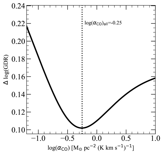
Figure 7: Scatter in the $\log(\mathrm{GDR})$ as a function of $\alpha_{\rm\atom{CO}{}{}}$. The $\log(\mathrm{GDR})$ scatter in our mapping area is minimized when the best-fit $\log(\alpha_{\rm\atom{CO}{}{}})=0.25$ is employed.

Given that dust and gas are well mixed and are linearly correlated, the total gas mass surface density $\Sigma_{\rm gas}$ can be estimated from the dust surface density, $\Sigma_{\rm dust}$ (see equation (1)). The molecular gas surface density, $\Sigma_{\rm mol}$, can be measured by including the contribution of the atomic surface density, $\Sigma_{\rm atom}$, which is derived from HI, to the total gas surface density $\Sigma_{\rm gas}(=\Sigma_{\rm atom}+\Sigma_{\rm mol})$. Conversely, $\Sigma_{\rm mol}$ is derived from CO by using a constant conversion factor, $\alpha_{\rm\atom{CO}{}{}}$, in which a factor of 1.36 is included to account for helium. Leroy et al. (2011) proposed a technique to solve $\mathrm{GDR}$ and $\alpha_{\rm\atom{CO}{}{}}$ simultaneously in Local Group galaxies by applying equation (1) to the maps of CO, HI, and IR emission under the assumptions that the $\mathrm{GDR}$ is constant over a region of galaxies and also does not vary between the atomic and molecular phases. The best $\alpha_{\rm\atom{CO}{}{}}$ in each target region can be determined by minimizing the scatter in $\mathrm{GDR}$ as a function of the $\alpha_{\rm\atom{CO}{}{}}$; moreover, the $\mathrm{GDR}$ is also determined simultaneously. Refining the technique, Sandstrom et al. (2013) derived the distribution of $\mathrm{GDR}$ and $\alpha_{\rm\atom{CO}{}{}}$ in nearby star-forming galaxies on the kpc scales, and showed $\mathrm{GDR}$ as an approximately linear function of the metallicity, with a slope of $\sim-0.85$, unlike $\alpha_{\rm\atom{CO}{}{}}$. Considering a metallicity gradient with a radius in the inner disk region of M83 ($<0.5R_{\rm 25}$) and with a slope of $-0.303~{}{\rm dex}~{}R_{25}^{-1}$ (Hernandez et al., 2019), it can establish that the assumption that the $\mathrm{GDR}$ is constant across the area studied in this work is reasonable.

Notably, the limitations of the method, wherein contamination from dust mixed with invisible components, such as opaque HI and ionized gas, are considered as negligible. However, Israel & Baas (2001) suggested that approximately half of all hydrogen is associated with ionized carbon in the central region of M 83. If a large amount of photodissociation products of CO, which is associated with the amount of hydrogen exists even in the disk region, then $\alpha_{\rm\atom{CO}{}{}}$ is overestimated by a factor of approximately 2.

$\mathrm{GDR}$ and dust opacity, $\kappa_{\rm\nu}$, may change within galaxies due to metallicity and gas density (e.g., Draine et al. (2007), Rémy-Ruyer et al. (2014), Galliano et al. (2018) and references therein). Considering a metallicity gradient in the studied area, the effect of the metallicity on GDR is expected to be minor in this work. However, as described in section 3.3, the variation in $\kappa_{\rm\nu}$ would introduce an uncertainly by less than a factor of 2 in $\mathrm{GDR}$ and $\alpha_{\rm\atom{CO}{}{}}$. In addition, uncertainties in $\mathrm{GDR}$ and $\alpha_{\rm\atom{CO}{}{}}$ can be attributed to the differences in dust emissivity between the molecular and atomic phases (e.g., a factor of $\sim 2$ for the Milky Way; Planck Collaboration et al. (2011b)); however, this effect can be neglected in this work because both phases in M83 exhibit similar emissivity, as reported by Clark et al. (2019). In conclusion, in this study, the derived $\mathrm{GDR}$ and $\alpha_{\rm\atom{CO}{}{}}$ have inherent uncertainties of at least a factor of 2.

Applying the same technique as Leroy et al. (2011), we searched for $\alpha_{\rm\atom{CO}{}{}}$ with the lowest scatter of the GDR in the galaxy, in the range of $\alpha_{\rm\atom{CO}{}{}}=0.05-50$ $M_{\Sol}$ pc^-2 (K km s^-1)^-1 with a step of 0.01 $M_{\Sol}$ pc^-2 (K km s^-1)^-1. At each value of $\alpha_{\rm\atom{CO}{}{}}$, the $\mathrm{GDRs}$ were calculated at all points in the [CI](1–0) mapping region. After dividing the $\mathrm{GDR}$ at each pixel by the mean $\mathrm{GDR}$ in the region, the scatter of the resulting values ($\Delta\log(\mathrm{DGR})$) was measured. Figure 7 presents the scatter in logarithm as a function of $\alpha_{\rm\atom{CO}{}{}}$. The minimum $\mathrm{GDR}$ scatter can be found at $\alpha_{\rm\atom{CO}{}{}}\approx 0.56$ $M_{\Sol}$ pc^-2 (K km s^-1)^-1 [$X_{\rm\atom{CO}{}{}}=0.26\times 10^{20}$ cm^-2(K km s^-1)^-1], corresponding to $\mathrm{GDR}\approx 20$. These values are smaller than the averaged values for nearby galaxies, $\alpha_{\rm\atom{CO}{}{}}\approx$3.1 $M_{\Sol}$ pc^-2 (K km s^-1)^-1 and $\mathrm{GDR}\approx 72$, reported by Sandstrom et al. (2013). Applying the standard $\alpha_{\rm\atom{CO}{}{}}(=3.1~{}M_{\Sol}~{}{\rm pc}^{-2}~{}({\rm K~{}km~{}s}^{-1})^{-1})$ to our datasets yields the $\mathrm{GDR}~{}\approx 110$ in the area studied ($r\leq\timeform{160"}$), which is compatible with the result ($\mathrm{GDR}\sim 70-180$) reported by Foyle et al. (2012). It has been reported that the conversion factor in the central region of M83, derived from the radiative transfer model using multiple CO and CO13 lines, becomes $X_{\rm\atom{CO}{}{}}=0.25\times 10^{20}$ cm^-2(K km s^-1)^-1, corresponding to $\alpha_{\rm\atom{CO}{}{}}\sim$0.5 $M_{\Sol}$ pc^-2 (K km s^-1)^-1 (Israel & Baas, 2001), which is consistent with our result. Nevertheless, in addition to the uncertainties as described before, the single temperature modified blackbody fitting that we used could lead to an overestimation of the dust mass under the high temperature environment, thereby yielding a low $\mathrm{GDR}$.

For applying the best fit $\alpha_{\rm\atom{CO}{}{}}$ and $\mathrm{GDR}$ values, the corresponding uncertainties in $\alpha_{\rm\atom{CO}{}{}}$ and $\mathrm{GDR}$ are estimated from the standard deviation of the values in the area and the systematic uncertainties arising from the uncertainty of the measured $\Sigma_{\atom{H}{}{}\emissiontype{I}}$, $I_{\rm\atom{CO}{}{}}$, and $\Sigma_{\rm dust}$ for applying the best fit $\alpha_{\rm\atom{CO}{}{}}$ and $\mathrm{GDR}$ values. The standard deviations become 0.26 $M_{\Sol}$ pc^-2 (K km s${}^{-1})^{-1}$ in $\alpha_{\rm\atom{CO}{}{}}$ and 4.54 in $\mathrm{GDR}$. The systematic uncertainties are calculated through a Monte Carlo test on the solutions by adding random noise to the measured $\Sigma_{\atom{H}{}{}\emissiontype{I}}$, $I_{\rm\atom{CO}{}{}}$, and $\Sigma_{\rm dust}$ according to the errors at each pixel. The calculation was repeated 100 times using the randomly perturbed data values and the standard deviations of the results were found to be 0.07 $M_{\Sol}$ pc^-2 (K km s${}^{-1})^{-1}$ for $\alpha_{\rm\atom{CO}{}{}}$ and 1.65 for the $\mathrm{GDR}$. Summing the uncertainties yields 0.27 $M_{\Sol}$ pc^-2 (K km s${}^{-1})^{-1}$ for $\alpha_{\rm\atom{CO}{}{}}$ and 4.83 for the $\mathrm{GDR}$.

Further, we adopted other techniques to search for the best $\alpha_{\rm\atom{CO}{}{}}$ and $\mathrm{GDR}$, e.g., ”Minimum fractional scatter in the $\mathrm{GDR}$” and ”Minimum $\chi^{2}$ of best-fit plane to $I_{\rm\atom{CO}{}{}}$, $N_{\rm HI}$, and $\Sigma_{\rm D}$”, introduced by Sandstrom et al. (2013). In addition to that, we searched for the best $\alpha_{\rm\atom{CO}{}{}}$ and $\mathrm{GDR}$ on the plane so as to minimize the summation of $(\Sigma_{{\rm gas,(dust)},i}-\Sigma_{{\rm gas,(atom+mol)},i})^{2}/(\delta\Sigma_{\rm gas,(dust)}^{2}+\delta\Sigma_{\rm gas,(atom+mol)}^{2})$, where $\Sigma_{{\rm gas,(dust)},i}=\mathrm{GDR}~{}\Sigma_{{\rm dust},i}$, $\Sigma_{{\rm gas,(atom+mol)},i}=\Sigma_{{\rm atom},i}+\alpha_{\rm\atom{CO}{}{}}~{}I_{{\rm\atom{CO}{}{}},i}$ at each pixel $i$, and $\delta\Sigma$ is the standard deviation in the region. The results are in a range of 0.5–0.65 $M_{\Sol}$ pc^-2 (K km s${}^{-1})^{-1}$ for $\alpha_{\rm\atom{CO}{}{}}$ and 19–25 for the $\mathrm{GDR}$, and the median values are $\alpha_{\rm\atom{CO}{}{}}=0.5$ $M_{\Sol}$ pc^-2 (K km s${}^{-1})^{-1}$ and $\mathrm{GDR}=20$, which will be used hereinafter.

4.2 Measurements of the [CI]-to-H₂ conversion factor $\alpha_{\rm[\atom{C}{}{}\emissiontype{I}]}$

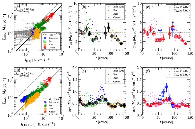
Figure 8: (a) Plots of $\Sigma_{\rm mol}$ as a function of $I_{\rm[\atom{C}{}{}\emissiontype{I}](1-0)}$, where the data with $I_{\rm[\atom{C}{}{}\emissiontype{I}](1-0)}<4~{}\sigma$ are represented by gray points, and the remaining graphs are represented in the same manner as in Figure 6. The best-fit relation with a fixed slope of unity to the data with $I_{\rm[\atom{C}{}{}\emissiontype{I}](1-0)}>4~{}\sigma$ is shown by the solid line, corresponding to $\alpha_{\rm[\atom{C}{}{}\emissiontype{I}]}\sim 3.8~{}[M_{\Sol}$ pc^-2 (K km s^-1)^-1]. The dashed line is the mean value of the local galaxies (7.3 [$M_{\Sol}$ pc^-2 (K km s^-1)^-1]) measured by Crocker et al. (2019). In panels (b) and (c), the radial variation of $\alpha_{\rm[\atom{C}{}{}\emissiontype{I}]}$ is plotted, but in (c), the data are separated into two halves using a division of $T_{\rm dust}=23$ K. The open boxes in panel (b) represent the values binned with a width of $r=\timeform{10"}$. The upward and downward triangles in panel (c) represent the values binned with a width of $r=\timeform{10"}$ as well, but for $T_{\rm dust}>23$ K and $\leq 23$ K, respectively. d) Plots of $\Sigma_{\rm mol}$ as a function of $I_{\rm\atom{CO}{}{}(1-0)}$. The best-fit relation with a fixed slope of unity is shown by the solid line, corresponding to $\alpha_{\rm\atom{CO}{}{}}\sim 0.5~{}[M_{\Sol}$ pc^-2 (K km s^-1)^-1]. The dashed line in panel (d) represents the averaged value $\alpha_{\rm\atom{CO}{}{}}\sim 3.1$ [$M_{\Sol}$ pc^-2 (K km s^-1)^-1] in nearby galaxies measured by Sandstrom et al. (2013). Panels (e) and (f) are the same as panel (b), and (c), but reflect the data for CO(1–0).

Assuming that the $\mathrm{GDR}$ is constant across the observed region and that [CI](1–0) traces the molecular gas, we measured the conversion factor of [CI] to the molecular gas surface density by using the following equation:

$$\alpha_{\rm[\atom{C}{}{}\emissiontype{I}]}I_{\rm[\atom{C}{}{}\emissiontype{I}]} = \Sigma_{\rm mol}$$ (9)

$$= \mathrm{GDR}~{}\Sigma_{\rm dust}-\Sigma_{\rm atom}.$$

Although the same method as that described in section 4.1 can be used to measure $\mathrm{GDR}$ and $\alpha_{\rm[\atom{C}{}{}\emissiontype{I}]}$, we note that the results obtained with this method are biased toward brighter [CI](1–0) (cf. Figure 5), resulting in their overestimation. Thus, we used $\mathrm{GDR}=20$, as obtained in section 4.1. Employing the $\mathrm{GDR}$ for the entire region, we derived $\alpha_{\rm[\atom{C}{}{}\emissiontype{I}]}$ by the least square fitting to the $\Sigma_{\rm mol}-I_{\rm[\atom{C}{}{}\emissiontype{I}]}$ relation above the 4 $\sigma$ noise level for $I_{\rm[\atom{C}{}{}\emissiontype{I}](1-0)}$ using the above equation. The slope corresponding to $\alpha_{\rm[\atom{C}{}{}\emissiontype{I}]}$ was $3.8\pm 0.1$ $M_{\Sol}$ pc^-2 (K km s${}^{-1})^{-1}$ with $R^{2}=0.90$ (black solid line in Figure 8(a)). The deviation from the fitting is however large at $I_{\rm[\atom{C}{}{}\emissiontype{I}]}\lesssim 7$ K km s^-1, particularly in the arm region. Thus if the the central region data are used, the fitting gives $\alpha_{\rm[\atom{C}{}{}\emissiontype{I}]}=4.0\pm 0.2$ $M_{\Sol}$ pc^-2 (K km s${}^{-1})^{-1}$. The conversion factors $\alpha_{\rm[\atom{C}{}{}\emissiontype{I}]}=7.3$ $M_{\Sol}$ pc^-2 (K km s${}^{-1})^{-1}$ for nearby galaxies (Crocker et al., 2019) and $\alpha_{\rm[\atom{C}{}{}\emissiontype{I}]}=4.9$ $M_{\Sol}$ pc^-2 (K km s${}^{-1})^{-1}$ for (U)LIRGs (Jiao et al., 2017) are larger than our results, although within the scatter. However, it must be noted that the conversion factor $\alpha_{\rm[\atom{C}{}{}\emissiontype{I}]}$ is generally determined using the molecular gas surface density based on $\alpha_{\rm\atom{CO}{}{}}$ (in addition, the intensity ratio of CO(2-1) to CO(1-0) in some cases) obtained from the literature. Through a linear regression fit for 30 nearby galaxies on the [CI](1–0) integrated intensity and H₂ column density that is derived from the radiative transfer models using multiple CO and CO13 lines, Israel (2020) has reported a lower conversion factor, $X_{[\atom{C}{}{}\emissiontype{I}]}=9\pm 2\times 10^{19}$ cm^-2 (K km s^-1)^-1, corresponding to $\alpha_{\rm[\atom{C}{}{}\emissiontype{I}]}=1.9$ $M_{\Sol}$ pc^-2 (K km s${}^{-1})^{-1}$, however, notably the average values for individual galaxies is almost twice as high. Moreover, Izumi et al. (2020) found a comparable value of $\alpha_{\rm[\atom{C}{}{}\emissiontype{I}]}=4.4$ $M_{\Sol}$ pc^-2 (K km s${}^{-1})^{-1}$ in the central region ($r<70$ pc) of NGC 7469 without using $\alpha_{\rm\atom{CO}{}{}}$, where they compared the line flux luminosity of [CI](1–0) with $M_{\rm mol}$, which is obtained by subtracting the stellar mass and the black hole mass from the dynamical mass by assuming a negligible dark matter. The consistency of $\alpha_{\rm[\atom{C}{}{}\emissiontype{I}]}$ in a different spatial scale implies the usefulness of [CI](1–0) as a molecular gas tracer if [CI](1–0) is bright, although further measurements are necessary.

The relationship between $I_{\rm\atom{CO}{}{}(1-0)}$ and $\Sigma_{\rm mol}$, which is derived using $\Sigma_{\rm dust}$ and $\mathrm{GDR}=20$ is plotted in figure 8(d). The best fitted slope of $\alpha_{\rm\atom{CO}{}{}}=0.49(\pm 0.01)$ $M_{\Sol}$ pc^-2 (K km s${}^{-1})^{-1}$ is derived with $R^{2}=0.9$, which is consistent with the value ($\alpha_{\rm\atom{CO}{}{}}=0.5$ $M_{\Sol}$ pc^-2 (K km s${}^{-1})^{-1}$) obtained in section 4.1. Overall, $I_{\rm\atom{CO}{}{}(1-0)}$ is well correlated with $\Sigma_{\rm mol}$; however, the data from the disk region, especially from the inter-arm, deviate by more than $0.3$ dex from the value of $\alpha_{\rm\atom{CO}{}{}}=0.49$ $M_{\Sol}$ pc^-2 (K km s${}^{-1})^{-1}$ relation, i.e., the value is larger than $\alpha_{\rm\atom{CO}{}{}}=0.49$ $M_{\Sol}$ pc^-2 (K km s${}^{-1})^{-1}$. It has been reported that $\alpha_{\rm\atom{CO}{}{}}$ is a function of the galactic radius (e.g., Nakai & Kuno (1995)). In Figure 8(d), $\alpha_{\rm\atom{CO}{}{}}$ is plotted as a function of the galactic radius, with binning of a width of $r=\timeform{10"}$; however, no systematic radial dependence is observed. To investigate the effect of the local excitation condition on $\alpha_{\rm\atom{CO}{}{}}$, we divided the data into two parts based on the dust temperature of 23 K (which is the dust temperature averaged over the galaxy) in Figures 8(c) and (f). The blue bins represent lower dust temperatures ($T_{\rm dust}\lesssim 23$ K), and the red bins represent higher temperatures ($T_{\rm dust}>23$ K). It is clearly visible that the higher values of $\alpha_{\rm\atom{CO}{}{}}$ are distributed in the low dust temperature region. Meanwhile, the optical depth of $\atom{CO}{}{}$, $\tau_{\rm\atom{CO}{}{}}$, can cause the variations in $\alpha_{\rm\atom{CO}{}{}}$, i.e., a small $\tau_{\rm\atom{CO}{}{}}$ leads to a large $\alpha_{\rm\atom{CO}{}{}}$ (e.g., Nakai & Kuno (1995)). In fact, Crosthwaite et al. (2002) reported that CO in the inter-arm region of M83 was optically thin, based on the high intensity ratio of CO(2–1)/CO(1–0) $(>1)$. Here, notably, $\tau_{\rm\atom{CO}{}{}}$ scales as $\tau_{\rm\atom{CO}{}{}}\propto\exp(h\nu/kT_{\rm ex})N_{\rm\atom{CO}{}{}}/\Delta v$, where $N_{\rm\atom{CO}{}{}}$ is the CO column density and $\Delta v$ the velocity width (e.g., Bolatto et al. (2013)). Considering the low temperature and narrow velocity width in the inter-arm region, a low CO abundance may cause the low optical depth, and consequently the higher values of $\alpha_{\rm\atom{CO}{}{}}$. The values of $\alpha_{\rm[\atom{C}{}{}\emissiontype{I}]}$ do not show the systematic radial dependence nor a significant difference between low and high temperatures. The dependences of $\alpha_{\rm\atom{CO}{}{}}$ and $\alpha_{\rm[\atom{C}{}{}\emissiontype{I}]}$ on the dust temperature are consistent with the results shown by Crocker et al. (2019). However, only a few [CI](1–0) data are available for low dust temperatures.

We compared the molecular gas mass ($M_{\rm mol,dust}$, $M_{\rm mol,CO}$, and $M_{\rm mol,[\atom{C}{}{}\emissiontype{I}]}$) in the studied area by applying $\mathrm{GDR}=20$, $\alpha_{\rm\atom{CO}{}{}}=0.5$ $M_{\Sol}$ pc^-2 (K km s${}^{-1})^{-1}$, and $\alpha_{\rm[\atom{C}{}{}\emissiontype{I}]}=3.8$ $M_{\Sol}$ pc^-2 (K km s${}^{-1})^{-1}$ to the dust surface density, including the atomic gas surface density and the integrated intensities of CO(1–0) and [CI](1–0). The resulting masses are summarized in Table 4.2. Although the mass in the entire area is consistent within the error, [CI](1–0) tends to underestimate the mass due to non-detection in regions with low dust temperature such as the inter-arm region.

Molecular Gas Mass Estimated using Dust, CO, and [CI] Mass[$10^{7}~{}M_{\Sol}$] all Center Arm Bar Interarm $M_{\rm mol,Dust}(\mathrm{GDR}=20)$ $8.3\pm 1.4$ $2.2\pm 0.3$ $1.4\pm 0.2$ $2.7\pm 0.5$ $1.2\pm 0.3$ $M_{\rm mol,CO}(\alpha_{\rm\atom{CO}{}{}}=0.5)$ $8.1\pm 0.2$ $2.1\pm 0.1$ $1.7\pm 0.1$ $2.8\pm 0.1$ $0.8\pm 0.1$ $M_{\rm mol,[\atom{C}{}{}\emissiontype{I}]}(\alpha_{\rm[\atom{C}{}{}\emissiontype{I}]}=3.8)$ $7.0\pm 1.9$ $2.1\pm 0.1$ $1.5\pm 0.4$ $2.1\pm 0.4$ $0.6\pm 0.3$

4.3 Excitation temperature, column density, and abundance of atomic carbon

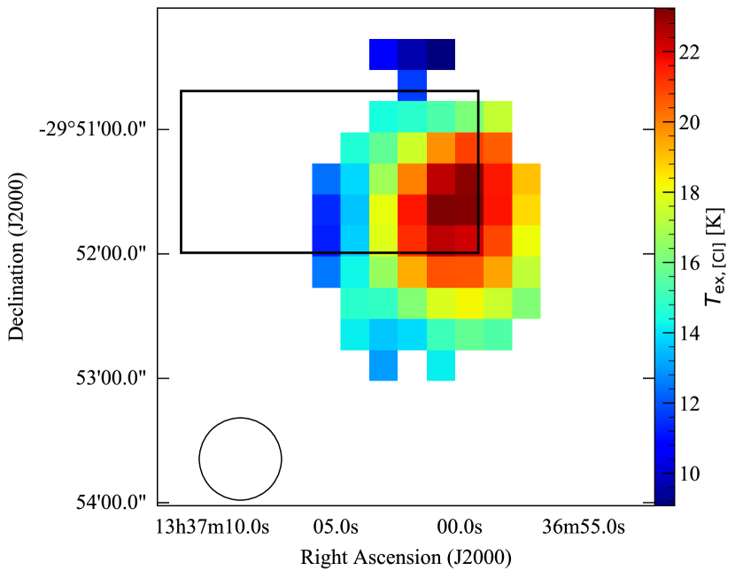
Figure 9: Spatial distribution of $T_{\rm ex}$ derived by substituting the ratio between [CI](1–0) and [CI](2–1), retrieved from the Very Nearby Galaxy Survey (VNGS) with Herschel/SPIRE FTS (Wu et al., 2015), into equation (14). The region indicated by the box represents the [CI](1–0) mapping area with ASTE.

In this section, we derive the excitation temperature ($T_{\rm ex}$) and column density of atomic carbon ($N_{\rm\atom{C}{}{}\emissiontype{I}}$), and the [CI]/[H₂] abundance ratio under the assumption that CI is in local thermodynamic equilibrium (LTE) and the two [CI] lines are optically thin.

The measured (background subtracted) radiation temperature from a region of uniform excitation temperature, $T_{\rm ex}$, is expressed as:

$$T_{\rm R}(T_{\rm ex},\nu)=\eta\left[J(T_{\rm ex},\nu)-J(T_{\rm CMB},\nu)\right]\left(1-e^{-\tau}\right),$$ (10)

where $\eta$ is the beam filling factor, $J(T,\nu)=(h\nu/k)/(e^{h\nu/kT}-1)$ is the brightness temperature, $T_{\rm CMB}$ is the cosmic microwave background temperature ($=2.73$ K), and $\tau$ is the optical depth. Assuming that the beam filling factor of [CI](1-0) is similar to that of [CI](2-1) and $T_{\rm ex}=T_{\rm ex,[\atom{C}{}{}\emissiontype{I}](1-0)}=T_{\rm ex,[\atom{C}{}{}\emissiontype{I}](2-1)}$, the ratio between $T_{\rm R,[\atom{C}{}{}\emissiontype{I}](1-0)}$ and $T_{\rm R,[\atom{C}{}{}\emissiontype{I}](2-1)}$ is

$$R_{\rm\atom{C}{}{}\emissiontype{I}_{21}/\atom{C}{}{}\emissiontype{I}_{10}} = \frac{J(T_{\rm ex},\nu_{\rm\atom{C}{}{}\emissiontype{I}_{21}})-J(T_{\rm CMB},\nu_{\rm\atom{C}{}{}\emissiontype{I}_{21}})}{J(T_{\rm ex},\nu_{\rm\atom{C}{}{}\emissiontype{I}_{10}})-J(T_{\rm CMB},\nu_{\rm\atom{C}{}{}\emissiontype{I}_{10}})}\frac{(1-e^{-\tau_{\rm\atom{C}{}{}\emissiontype{I}_{21}}})}{(1-e^{-\tau_{\rm\atom{C}{}{}\emissiontype{I}_{10}}})}$$ (11)

$$= \mathcal{K}\frac{(1-e^{-\tau_{\rm\atom{C}{}{}\emissiontype{I}_{21}}})}{(1-e^{-\tau_{\rm\atom{C}{}{}\emissiontype{I}_{10}}})},$$

where $\mathcal{K}\equiv(J(T_{\rm ex},\nu_{\rm\atom{C}{}{}\emissiontype{I}_{21}})-J(T_{\rm CMB},\nu_{\rm\atom{C}{}{}\emissiontype{I}_{21}}))/(J(T_{\rm ex},\nu_{\rm\atom{C}{}{}\emissiontype{I}_{10}})-J(T_{\rm CMB},\nu_{\rm\atom{C}{}{}\emissiontype{I}_{10}}))$. Under the assumption that two [CI]  lines are optically thin ($\tau_{\rm\atom{C}{}{}\emissiontype{I}_{10}},\tau_{\rm\atom{C}{}{}\emissiontype{I}_{21}}\ll 1$), equation (11) can be described as

$$R_{\rm\atom{C}{}{}\emissiontype{I}_{21}/\atom{C}{}{}\emissiontype{I}_{10}} = \mathcal{K}~{}\frac{\tau_{\rm\atom{C}{}{}\emissiontype{I}_{21}}}{\tau_{\rm\atom{C}{}{}\emissiontype{I}_{10}}}.$$ (12)

The optical depth of the [CI] line is given by

$$\tau_{\rm ul}=\frac{\rm c^{3}}{8\pi\nu_{\rm ul}^{3}}N_{\rm\atom{C}{}{}\emissiontype{I}}\frac{g_{\rm u}}{Q}e^{-E_{\rm u}/kT_{\rm ex}}A_{\rm ul}\frac{1}{\Delta V}(e^{h\nu_{\rm ul}/kT_{\rm ex}}-1),$$ (13)

where the subscripts $u$ and $l$ denote the upper and lower energy levels, $c$ is the speed of light, $\nu_{\rm ul}$ is the frequency corresponding to the transition, $N_{\rm\atom{C}{}{}\emissiontype{I}}$ is the total column density of CI, $g_{\rm u}$ is the statistical weight, $Q$ is the partition function, $E_{\rm u}$ is the energy of the level (i.e., $E_{1}/k=23.6$ K and $E_{2}/k=62.5$ K for the ${}^{3}P_{1}$ and ${}^{3}P_{2}$ levels, respectively), $k$ is the Boltzmann constant, $A_{\rm ul}$ is the Einstein coefficient ($A_{10}=10^{-7.09725}$ s^-1 and $A_{21}=10^{-6.57415}$ s^-1, Müller et al. (2005)), and $\Delta V$ is the velocity width (see appendix A of Salak et al. (2019) for more details of the derivation). Substituting equation (13) into equation (12) under the assumption that $\Delta V$ of [CI](2–1) is the same as that of [CI](1–0), we obtain

$$R_{\rm\atom{C}{}{}\emissiontype{I}_{21}/\atom{C}{}{}\emissiontype{I}_{10}} = 1.25~{}\mathcal{K}~{}\left(\frac{e^{-62.5/T_{\rm ex}}}{e^{-23.6/T_{\rm ex}}}\right)\left(\frac{e^{h\nu_{21}/T_{\rm ex}}-1}{e^{h\nu_{10}/T_{\rm ex}}-1}\right).$$ (14)

Utilizing the integrated intensity ratio of [CI](1–0) and [CI](2–1), $T_{\rm ex}$ can be derived from equation (14). We retrieved the [CI](1–0) and [CI](2–1) data of M83 from the VNGS with the Fourier transform spectrometer (FTS) of Herschel/SPIRE (Wu et al., 2015), although the [CI] data do not wholly cover our mapping area, e.g., the spiral arm. Nevertheless, the archival data are convolved to a common spatial resolution of 417 and the pixels on the edge of each convolved map are truncated (cf. Figure 1 in Wu et al. (2015)). The $T_{\rm ex}$ distribution of M83 is shown in Figure 9, in which our mapping area is indicated by a black box. The mean excitation temperature in our mapping area is $T_{\rm ex}=18\pm 3$ K. The temperature of $T_{\rm ex}\sim 23$K in the central region decreases with the radius and reaches to $\lesssim 15$ K in the disk region.

The column density of atomic carbon gas $N_{\rm\atom{C}{}{}\emissiontype{I}}$ in the LTE is given as

$$N_{\rm\atom{C}{}{}\emissiontype{I}}=\frac{8\pi\nu_{\rm 10}^{3}}{hc^{3}A_{10}}\frac{Q}{g_{1}}e^{E_{1}/T_{\rm ex}}I_{\rm[\atom{C}{}{}\emissiontype{I}]}.$$ (15)

For $T_{\rm ex}=$13, 18, and 23 K, the column densities in the mapping area are $N_{\rm\atom{C}{}{}\emissiontype{I}}=(7.4\pm 1.5)\times 10^{16}$ cm^-2, $(5.7\pm 1.2)\times 10^{16}$ cm^-2, and $(5.3\pm 1.1)\times 10^{16}$ cm^-2, respectively, that are obtained by using our integrated intensity of [CI](1–0). $N_{\rm\atom{C}{}{}\emissiontype{I}}$ for each region is summarized in Table 4.3. In addition, the [CI]/[H₂] abundance ratio can be derived using the H₂ column density, $N_{\rm\atom{H}{}{}_{2}}(=4.59\times 10^{19}~{}\Sigma_{\rm mol}$). The mean abundance ratio in the mapping area is $(6.9\pm 1.8)\times 10^{-5}$ for $T_{\rm ex}=18$ K. This is comparable with the estimates of $\sim 7\times 10^{-5}$ in the central region of the starburst galaxy NGC 1808 (Salak et al., 2019) and $8.3\pm 3.0\times 10^{-5}$ for local (U)LIRGs (Jiao et al., 2017); however, our value is higher than the abundance of $2.5\pm 1.0\times 10^{-5}$ that is obtained as the average of the nearby galaxies that host starbursts and AGNs (Jiao et al., 2019). Adopting $T_{\rm ex}$ of 23, 18, 13 K for the central region, the disk (bar and arm) region, and the inter-arm region (Figure 9), respectively, the abundance ratio is found to be $\sim 7\times 10^{-5}$ within a range of 0.1 dex.

CI Column densities and Abundance Ratios of CI and H₂ in LTE all Center Bar Arm Interarm $T_{\rm ex}=13$ K $N_{\rm C}$ [10¹⁶ cm^-2] $7.4\pm 1.5$ $41.8\pm 2.6$ $7.2\pm 1.5$ $5.3\pm 1.4$ $2.7\pm 1.5$ [C]/[H₂] ($\times 10^{-5}$) $8.9\pm 2.4$ $9.9\pm 1.5$ $8.2\pm 2.2$ $11.4\pm 3.6$ $5.6\pm 3.3$ $T_{\rm ex}=18$ K $N_{\rm C}$ [10¹⁶ cm^-2] $5.7\pm 1.2$ $32.4\pm 2.0$ $5.6\pm 1.1$ $4.1\pm 1.1$ $2.1\pm 1.1$ [C]/[H₂] ($\times 10^{-5}$) $6.9\pm 1.8$ $7.7\pm 1.2$ $6.3\pm 1.7$ $8.9\pm 2.8$ $4.3\pm 2.6$ $T_{\rm ex}=23$ K $N_{\rm C}$ [10¹⁶ cm^-2] $5.3\pm 1.1$ $29.8\pm 1.8$ $5.2\pm 1.1$ $3.8\pm 1.0$ $1.9\pm 1.0$ [C]/[H₂] ($\times 10^{-5}$) $6.3\pm 1.7$ $7.1\pm 1.1$ $5.8\pm 1.6$ $8.2\pm 2.6$ $4.0\pm 2.4$

4.4 Comparison of [CI](1–0) stacked intensity with dust temperature

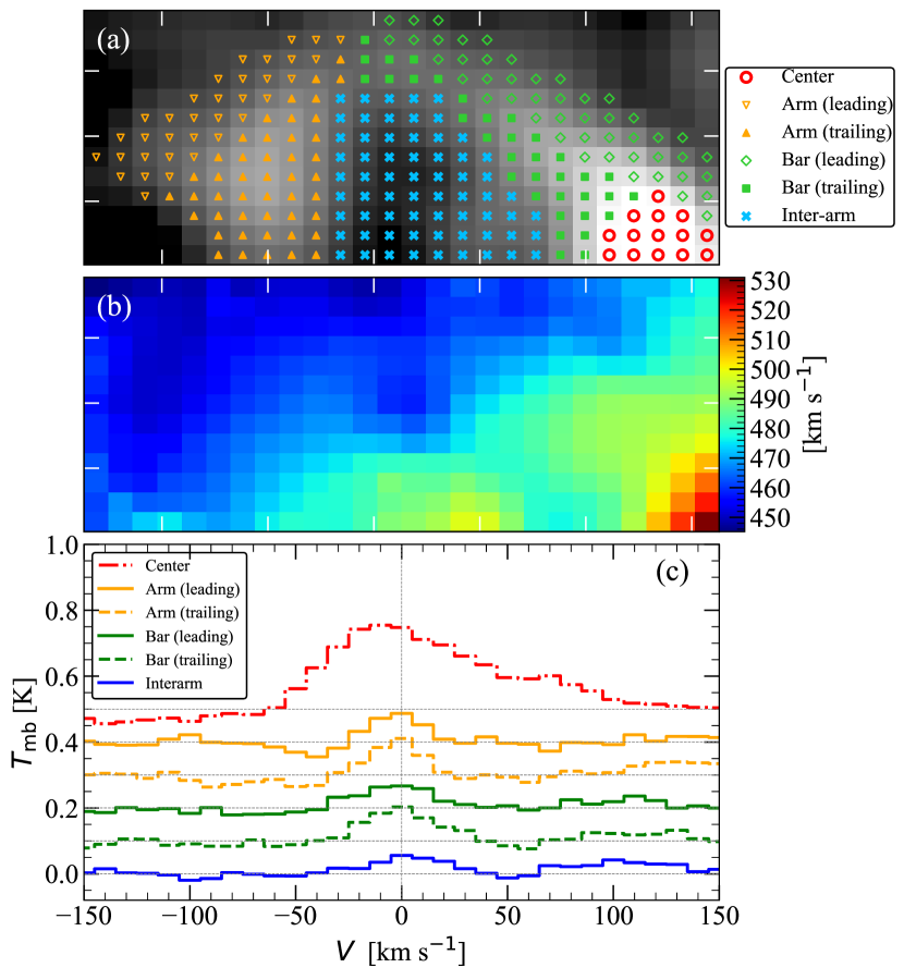
Figure 10: (a) Integrated intensity maps of CO(1–0) overlaid with the region for the stacking analysis. The center is represented by circles, leading side arm by downward triangles, trailing side arm by upward triangles, leading side bar by diamonds, trailing side bar by squares, and inter-arm by crosses. (b) CO(1–0) velocity field map derived from intensity-weighted mean velocities. (c) [CI](1–0) spectra stacked in each galactic structure represented in (a). The vertical axis depicts the main-beam brightness temperature in K.

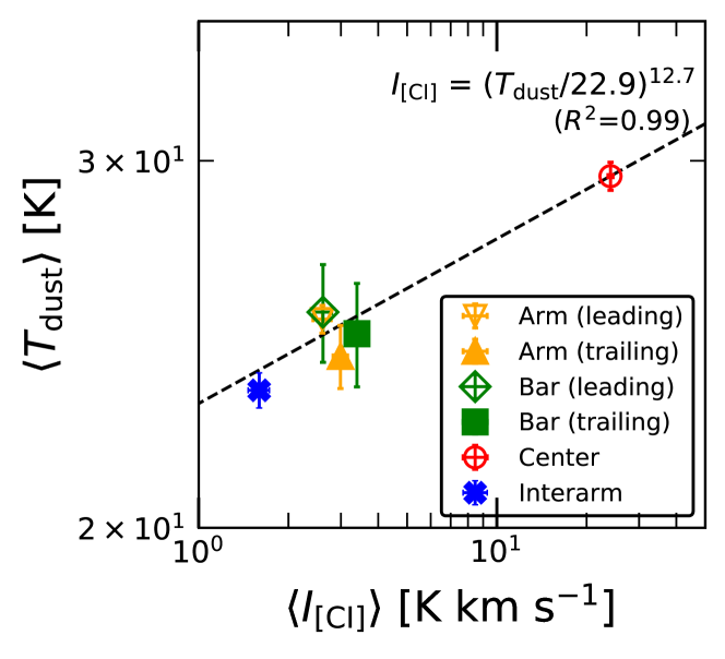
Figure 11: Plot of $T_{\rm dust}$ averaged over each of the six regions represented in Figure 10 as a function of the stacked integrated intensity of [CI](1–0), $\langle I_{\rm[\atom{C}{}{}\emissiontype{I}]}\rangle$. The dashed line represents the best-fit relation of $\langle I_{\rm[\atom{C}{}{}\emissiontype{I}]}\rangle=\left(\langle T_{\rm dust}\rangle/22.9\right)^{12.7}$. The symbols are the same as those in Figure 10.

In sections 3.3, we have mentioned the possibility that [CI](1–0) is sensitive to local excitations; however, much less [CI](1–0) data are available at a low $T_{\rm dust}$ region, such as in the inter-arm region. To measure the dependence, we employed a stacking technique (e.g., Morokuma-Matsui et al. (2015)) using the intensity-weighted velocity field map of CO(1–0) as a reference (Figure 10(b)). We split the galaxy into six characteristic galactic structures: (1) center, (2) leading side of the arm, (3) trailing side of the arm, (4) leading side of the bar, (5) trailing side of the bar, and (6) inter-arm, as shown in Figure 10(a). For the process, the [CI](1–0) spectra were first shifted along the velocity axis, according to the CO(1-0) velocity field. Next, the velocity-shifted spectra were averaged in each region with equal weights for each velocity pixel. However, this analysis is not very effective for [CI](1–0) if its velocity is different from that of CO(1–0).

The resulting stacked [CI](1–0) spectra are shown in Figure 10. [CI](1–0) line was detected in all regions with S/N $>5$. We examined the relation between the stacked spectral intensity ($\langle I_{\rm[\atom{C}{}{}\emissiontype{I}]}\rangle$) and the dust temperature averaged over the corresponding regions ($\langle T_{\rm dust}\rangle$). From figure 11, we find that the stacked intensity is a function of the dust temperature. The $\langle I_{\rm[\atom{C}{}{}\emissiontype{I}]}\rangle$–$\langle T_{\rm dust}\rangle$ relationship is fitted by $\langle I_{\rm[\atom{C}{}{}\emissiontype{I}]}\rangle=\left(\langle T_{\rm dust}\rangle/22.9\pm 0.4\right)^{12.7\pm 0.9}$ with $R^{2}=0.99$. The strong correlation between $\langle I_{\rm[\atom{C}{}{}\emissiontype{I}]}\rangle$ and $\langle T_{\rm dust}\rangle$ indicates that [CI](1–0) is sensitive to the dust temperature, especially for $T_{\rm dust}\gtrsim 23$ K (cf. $E/k=23.6$ K for the excitation energy of the upper level of [CI](1–0)). The dust temperature is associated with the external far ultraviolet (FUV) flux. Assuming that the FUV flux incident on a cloud surface is equal to the outgoing flux of dust radiation from the cloud, the UV radiation can be expressed as a function of $T_{\rm dust}$ in units of the Habing Field, i.e., $G_{0}=1.6\times 10^{-3}$ ergs cm^-2 s^-1 (e.g., $G/G_{0}=(T_{\rm dust}/12.2~{}{\rm K})^{5}$, Hollenbach et al. (1991)). Classical PDR models have suggested that CO is easily photodissociated by FUV photons, arising from massive stars (e.g., Tielens & Hollenbach (1985), van Dishoeck & Black (1988), Hollenbach et al. (1991), Kaufman et al. (1999)); hence, CI predominantly exists in the surfaces of the UV-irradiated molecular clouds. Meanwhile, the models have argued the weak dependence of the [CI](1–0) intensity on the dust temperature, which fails to explain our results. We note that the limited range of $T_{\rm dust}$, measured by this work, may have resulted in the observed high exponential dependence of [CI](1–0) intensity. To confirm this dependence, further measurements are required in a much wider range of $T_{\rm dust}$.

We demonstrated that [CI](1–0) was distributed outside the CO gas in the spiral arm, although the [CI](1–0) distribution in the central region was similar to that of the CO, which is consistent with the previous studies. Moreover, the enhanced [CI](1–0) on the leading side (outer region) of the arm was in good agreement with the warm dust traced by 70 $\mu$m, atomic gas traced by HI, OB stars traced by H$\alpha$, and interstellar radiation field indicated by the distribution of $T_{\rm dust}$. These results suggest that the atomic carbon is a photodissociation product of CO. Consequently, [CI](1–0) is less reliable in tracing the bulk of ”cold” molecular gas in the disk of the galaxy, although it is correlated with CO in the central region.

Recent simulations have suggested that cosmic rays can induce the destruction of CO, thus leaving behind CI-rich molecular gas (e.g., Bisbas et al. (2015), Glover et al. (2015), Papadopoulos, et al. (2018)). Furthermore, the dust temperature was found to be inversely correlated with metallicity above $12+\log(\atom{O}{}{}/\atom{H}{}{})\sim 8$, increasing from $T_{\rm dust}\sim 22$ K near the solar metallicity ($12+\log(\atom{O}{}{}/\atom{H}{}{})\sim 8.7$) to 35 K near a metallicity of 8 (Engelbracht et al., 2008). If the reduced dust shielding in the cloud in the galaxies with low metallicity causes CO to be preferentially photo-dissociated relative to H₂, the formation of CI (and CII)-dominated H₂ is expected rather than CO. The increasing trend in the ratio of $I_{\rm[\atom{C}{}{}\emissiontype{I}]}/I_{\rm\atom{CO}{}{}}$ for decreasing metallicity in the range of $12+\log(\atom{O}{}{}/\atom{H}{}{})\sim 8-9.1$ has been reported by Bolatto et al. (2000). Although CO is a good tracer of the total cold molecular gas mass in galaxies, [CI](1–0) could be a substitute for CO only in relatively hot regions, such as galactic centers and star-forming regions, and low-metallicity environments, as shown in this work and the previous studies (e.g., Israel (2020)).

5 Summary

We have presented the image of the northern part of the spiral galaxy M83 in [CI](1–0) emission, and compared the [CI](1–0) distribution with CO and molecular gas traced by dust across the galactic structures, including the center, bar, arm, and inter-arm, for the first time. The results of our study are summarized as follows:

1. We observed the nearby galaxy M83 in [CI](1–0) with ASTE. [CI](1–0) is detected in the central as well as the bar and arm regions. The [CI](1–0) distribution in the central region is similar to the distributions of CO(1–0), CO(3–2), and CO13(1–0). In the arm region, [CI](1–0) is found to be in the leading side, which is consistent with the results of HI and 70 $\mu$m rather than CO(1–0) and 250 $\mu$m.

2. The [CI](1–0) line luminosity is well correlated with the CO(1–0), C13O(1–0), and CO(3–2) luminosities in the central region; however, it is weak or not correlated in the disk region. Although the relationship obtained using the data only in the central region is in good agreement with the values in the literature, the slope is steeper when all data including those of the central and disk regions are used.

3. We derived the distributions of $T_{\rm dust}$ and $\Sigma_{\rm dust}$ through the modified blackbody fitting to the surface brightness at 70, 160, and $250~{}\mu$m. The distribution of $T_{\rm dust}$ was nearly consistent with [CI] in the arm and central regions but was offset from the leading edges of CO and dust in the bar and arm regions. The distribution of $\Sigma_{\rm dust}$ was much more consistent with CO(1–0) than with [CI](1–0).

4. We estimated the CO-to-H₂ conversion factor $\alpha_{\rm\atom{CO}{}{}}$ and gas-to-dust ratio $\mathrm{GDR}$ simultaneously to minimize the scatter in the $\mathrm{GDR}$ values in the mapping region. We calculated $\alpha_{\rm\atom{CO}{}{}}=0.5~{}M_{\Sol}$ pc^-2 (K km s^-1)^-1 and $\mathrm{GDR}=20$. The value of $\alpha_{\rm\atom{CO}{}{}}$ is consistent with that derived from the radiative transfer model in the central region of M83 (Israel & Baas, 2001); however, it is lower than the average $\alpha_{\rm\atom{CO}{}{}}=3.1~{}M_{\Sol}$ pc^-2 (K km s^-1)^-1 for the disks of nearby star-forming galaxies (Sandstrom et al., 2013). In addition to the uncertainties of at least factor of 2 in $\mathrm{GDR}$ and $\alpha_{\rm\atom{CO}{}{}}$, the single-temperature modified black body fitting adopted by us could cause overestimation of the dust mass in a high-temperature environment, yielding the low $\mathrm{GDR}$ and $\alpha_{\rm\atom{CO}{}{}}$. Applying $\mathrm{GDR}=20$, the [CI]-to-H₂ conversion factor $\alpha_{[\atom{C}{}{}\emissiontype{I}]}$ = 3.8$~{}M_{\Sol}$ pc^-2 (K km s^-1)^-1 was derived through the least square fitting to the $\Sigma_{\rm mol}$–$I_{\rm[\atom{C}{}{}\emissiontype{I}]}$ relation. The molecular gas masses in the entire area estimated through dust, CO, and [CI] were consistent within error; however, [CI](1–0) tended to underestimate the mass in the low-$T_{\rm dust}$ regions, such as the inter-arm.

5. We derived the [CI] excitation temperature, $T_{\rm ex}$, by using the two [CI] lines (${}^{3}P_{1}-^{3}P_{0}$ and ${}^{3}P_{2}-^{3}P_{1}$) obtained with the Herschel. The temperature of $T_{\rm ex}\sim 23$ K in the central region decreases with the radius and becomes less than $15$ K in the disk region. Given the mean temperature $T_{\rm ex}\sim 18$ K in our mapping area, the column density and abundance of CI were $N_{\rm\atom{C}{}{}}=(5.7\pm 1.2)\times 10^{16}$ cm^-2 and $[{\rm\atom{C}{}{}}]/[{\rm\atom{H}{}{}_{2}}]=(6.9\pm 1.8)\times 10^{-5}$, respectively. Adopting an appropriate $T_{\rm ex}$ in each region (center, disk, arm, inter-arm) yielded a constant abundance of $\sim 7\times 10^{-5}$ within a range of 0.1 dex in all regions.

6. By applying the stacking analysis with aligned velocity, by referring to the CO(1–0) velocity field, the [CI](1–0) spectra in the central and disk regions (the leading and trailing sides of the arm and bar, and inter-arm) were detected. The stacked intensity of [CI](1–0) is strongly correlated to $T_{\rm dust}$. This strong correlation between $\langle I_{\rm[\atom{C}{}{}\emissiontype{I}]}\rangle$ and $\langle T_{\rm dust}\rangle$ indicates that [CI](1–0) is sensitive to the dust temperature. In addition, a comparison of the distributions of [CI](1–0), CO, $T_{\rm dust}$, and other lines (e.g., HI and H$\alpha$) suggests that the atomic carbon is a photodissociation product of CO. Our results reveal that [CI](1–0) is less reliable in tracing the bulk of ”cold” molecular gas in the disk of the galaxy, although it could be a substitute for CO only in regions with relatively warm and/or [CI](1–0)-bright intensity, such as at the galactic center.

We would like to thank the referee, Frank Israel, for valuable comments on the manuscript. The ASTE telescope is operated by National Astronomical Observatory of Japan (NAOJ). This paper makes use of the following ALMA data: ADS/JAO.ALMA#2012.1.00762.S, ADS/JAO.ALMA#2015.1.01593.S. ALMA is a partnership of ESO (representing its member states), NSF (USA), and NINS (Japan), together with NRC (Canada), MOST and ASIAA (Taiwan), and KASI (Republic of Korea), in cooperation with the Republic of Chile. The Joint ALMA Observatory is operated by ESO, AUI/NRAO and NAOJ. The VNGS data was accessed through the Herschel Database in Marseille (HeDaM - http://hedam.lam.fr) operated by CeSAM and hosted by the Laboratoire d’Astrophysique de Marseille. The National Radio Astronomy Observatory is a facility of the National Science Foundation operated under cooperative agreement by Associated Universities, Inc. This research has made use of the NASA/IPAC Extragalactic Database (NED), which is operated by the Jet Propulsion Laboratory, California Institute of Technology, under contract with the National Aeronautics and Space Administration. Data analysis was in part carried out on the Multi-wavelength Data Analysis System operated by the Astronomy Data Center (ADC), National Astronomical Observatory of Japan. This work was supported by JSPS KAKENHI Grant Numbers JP20K04034, JP19H00702.

References

- Bendo et al. (2012) Bendo, G. J., Boselli, A., Dariush, A., et al. 2012, MNRAS, 419, 1833.
- Bisbas et al. (2015) Bisbas, T. G., Papadopoulos, P. P., & Viti, S. 2015, ApJ, 803, 37.
- Bolatto et al. (2000) Bolatto, A. D., Jackson, J. M., Kraemer, K. E., & Zhang, X. 2000, ApJ, 541, L17.
- Bolatto et al. (2013) Bolatto, A. D., Wolfire, M., & Leroy, A. K. 2013, ARA&A, 51, 207.
- Comte (1981) Comte, G. 1981, A&AS, 44, 441.
- Clark et al. (2019) Clark, C. J. R., De Vis, P., Baes, M., et al. 2019, MNRAS, 489, 5256.
- Crocker et al. (2019) Crocker, A. F., Pellegrini, E., Smith, J.-D. T., et al. 2019, ApJ, 887, 105.
- Crosthwaite et al. (2002) Crosthwaite, L. P., Turner, J. L., Buchholz, L., Ho, P. T. P., & Martin, R. N. 2002, AJ, 123, 1892.