Rissanen Data Analysis:
Examining Dataset Characteristics via Description Length
Abstract
We introduce a method to determine if a certain capability helps to achieve an accurate model of given data. We view labels as being generated from the inputs by a program composed of subroutines with different capabilities, and we posit that a subroutine is useful if and only if the minimal program that invokes it is shorter than the one that does not. Since minimum program length is uncomputable, we instead estimate the labels’ minimum description length (MDL) as a proxy, giving us a theoretically-grounded method for analyzing dataset characteristics. We call the method Rissanen Data Analysis (RDA) after the father of MDL, and we showcase its applicability on a wide variety of settings in NLP, ranging from evaluating the utility of generating subquestions before answering a question, to analyzing the value of rationales and explanations, to investigating the importance of different parts of speech, and uncovering dataset gender bias.111Code and results at https://github.com/ethanjperez/rda, along with a script to conduct RDA on your own dataset.
1 Introduction
In many practical learning scenarios, it is useful to know what capabilities would help to achieve a good model of the data. According to Occam’s Razor, a good model is one that provides a simple explanation for the data (Blumer et al., 1987), which means that the capability to perform a task is helpful when it enables us to find simpler explanations of the data. Kolmogorov complexity Kolmogorov (1968) formalizes the notion of simplicity as the length of the shortest program required to generate the labels of the data given the inputs. In this work, we estimate the Kolmogorov complexity of the data by approximately computing the data’s Minimum Description Length (MDL; Rissanen, 1978), and we examine how the data complexity changes as we add or remove different features from the input. We name our method Rissanen Data Analysis (RDA) after the father of the MDL principle, and we use it to examine several open questions about popular datasets, with a focus on NLP.
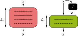
We view a capability as a function that transforms in some way (e.g., adding a feature), and we say that is helpful if invoking it leads to a shorter minimum program for mapping to the corresponding label in a dataset (see Fig. 1 for an illustration). Finding a short program is equivalent to finding a compressed version of the labels given the inputs, since the program can be run to generate the labels. Thus, we can measure the shortest program’s length by estimating the labels’ maximally compressed length, or Minimum Description Length (MDL; Rissanen, 1978; Grünwald, 2004). While prior work in machine learning uses MDL for model optimization Hinton and van Camp (1993), selection Yogatama et al. (2019), and model probing Voita and Titov (2020); Lovering et al. (2021), we use MDL for a very different end: to understand the data itself (“dataset probing”).
RDA addresses empirical and theoretical inadequacies of prior data analysis methods. For example, two common approaches are to evaluate the performance of a model when the inputs are modified or ablated (1) at training and test time or (2) at test time only. Training time input modification has been used to evaluate the usefulness of the capability to decompose a question into subquestions Min et al. (2019b); Perez et al. (2020), to access the image for image-based question-answering Antol et al. (2015); Zhang et al. (2016a), and to view the premise when detecting if it entails a hypothesis Gururangan et al. (2018); Poliak et al. (2018); Tsuchiya (2018). However, these works evaluate performance only on held-out dev examples, a fraction of all examples in the dataset, which also are often drawn from a different distribution (e.g., in terms of quality). To understand what datasets teach our models, we must examine the entire dataset, also giving us more examples for evaluation. Furthermore, a capability’s usefulness to a model in high-data regimes does not necessarily reflect its usefulness in low-data regimes, which have increasingly become of interest Lake et al. (2017); Guzmán et al. (2019); Brown et al. (2020). Test time ablation has been used to evaluate the capability to view word order Pham et al. (2020); Sinha et al. (2020); Gupta et al. (2021) or words of different types Sugawara et al. (2020), or to perform multi-hop reasoning Jiang and Bansal (2019). However, it is hard to rule out factors that may explain poor performance (e.g., distribution shift) or good performance (e.g., other ways to solve a problem). Here, we examine an intrinsic property of the dataset (MDL) and provide a theoretical argument justifying why it is the right measure to use.
We use RDA to provide insights on a variety of datasets. First, we verify that description length is reduced when we invoke a capability that is known to be helpful on a carefully-controlled synthetic task. Next, we examine HotpotQA Yang et al. (2018), a benchmark for answering questions, where prior work has both claimed that decomposing questions into subquestions is helpful Min et al. (2019b); Perez et al. (2020) and called such claims into question Min et al. (2019a); Jiang and Bansal (2019); Chen and Durrett (2019). RDA shows that subquestions are indeed helpful and exposes how evaluation procedures in prior work may have caused the value of question decomposition to be underestimated. We then evaluate if explanations are useful for recognizing textual entailment using the e-SNLI dataset Camburu et al. (2018). Both written explanations and decision-relevant keyword markings (“rationales”) are helpful, but rationales are more useful than explanations. Lastly, we examine a variety of popular NLP tasks, evaluating the extent to which they require relying on word order, different types of words, and gender bias. Overall, our results show that RDA can be used to answer a broad variety of questions about datasets.
2 Rissanen Data Analysis
How can we determine whether or not a certain capability is helpful for building a good model of the data? To answer this question, we view a dataset with inputs and labels as generated by a program that maps . Let the length of the shortest such program be , the data’s Kolmogorov complexity. We view a capability as a function that maps to a possibly helpful output , with being the length of the shortest label-generating program when access to is given. We say that is helpful exactly when:
| (1) |
2.1 Minimum Description Length
To use Eq. 1 in practice, we need to find the shortest program , which is uncomputable in general. However, because is a program that generates given , we can instead consider any compressed version of , along with an accompanying decompression algorithm that produces given and the compressed . To find , then, we find the length of the maximally compressed , or Minimum Description Length (MDL; Rissanen, 1978). While MDL is not computable, just like Kolmogorov complexity, many methods have been proposed to estimate MDL by restricting the set of allowed compression algorithms (see Grünwald, 2004, for an overview). These methods are all compatible with RDA, and here, we use online (or prequential) coding (Rissanen, 1984; Dawid, 1984), an effective method for estimating MDL when used with deep learning (Blier and Ollivier, 2018).
2.2 Online Coding
To examine how much can be compressed, we look at the minimum number of bits (minimal codelength) needed by a sender Alice to transmit to a receiver Bob, when both share . Without loss of generality, we assume is an element from a finite set. In online coding, Alice first sends Bob the learning algorithm , including the model architecture, trainable parameters , optimization procedure, hyperparameter selection method, initialization scheme, random seed, and pseudo-random number generator. Alice and Bob each initialize a model using the random seed and pseudo-random number generator, such that both models are identical.
Next, Alice sends each label one by one. Shannon (1948) showed that there exists a minimum code to send with bits when Alice and Bob share and . After Alice sends , Alice and Bob use to train a better model on to get shorter codes for future labels. The codelength for is then:
| (2) |
Intuitively, is the area under the “online” learning curve that shows how the cross-entropy loss goes down as training size increases. Overall, Alice’s message consists of plus the label encoding ( bits). When Alice and Bob share , Alice’s message consists of plus bits to encode the labels with a model . is helpful when the message is shorter with than without, i.e., when:
2.3 Implementation with Block-wise Coding
The online code in Eq. 2 is expensive to compute. It has a computational complexity that is quadratic in (assuming linear time learning), which is prohibitive for large and compute-intensive . Following Blier and Ollivier (2018), we upper bound online codelength by having Alice and Bob only train the model upon having sent labels. Alice thus sends all labels in a “block” at once using , giving codelength:
Since has no training data, Alice sends Bob the first block using a uniform prior.
Alleviating the sensitivity to learning algorithm
To limit the effect of the choice of learning algorithm , we may ensemble many model classes. To do so, we have Alice train models of different classes and send the next block’s labels using the model that gives the shortest codelength. To tell Bob which model to use to decompress a block’s labels, Alice also sends bits per block , adding to MDL. In this way, MDL relies less on the behavior of a single model class.
2.4 Experimental Setup
To evaluate MDL, we first randomly sort examples in the dataset. We use blocks where and such that is constant (log-uniform spacing). To train a model on the first blocks, we split the available examples into train (90%) and dev (10%) sets, choosing hyperparameters and early stopping epoch using dev loss (codelength). We otherwise follow each model’s training strategy and hyperparameter ranges as suggested by its original paper. We then evaluate the codelength of the -th block. As a baseline, we show , the codelength with the label prior as .
MDL is impacted by random factors such as the order of examples, model initialization, and randomness during training. Thus, we report the mean and std. error of MDL over 5 random seeds. For efficiency, we only sweep over hyperparameters for the first random seed and reuse the best hyperparameters for the remaining seeds. For all experiments, our code and reported codelengths are publicly available at https://github.com/ethanjperez/rda, along with a short Python script to conduct RDA with your own models and datasets.
3 Validating Rissanen Data Analysis
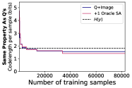
Having described our setup, we now verify that holds in practice when using an that we know is helpful. To this end, we use CLEVR Johnson et al. (2017), an synthetic, image-based question-answering (QA) dataset. Many CLEVR questions were carefully designed to benefit from answering subquestions. For example, to answer the CLEVR question “Are there more cubes than spheres?” it helps to know the answer to the subquestions “How many cubes are there?” and “How many spheres are there?” We hypothesize that MDL decreases as we give a model answers to subquestions.
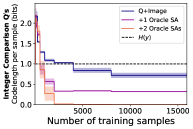
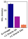
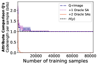
We test our hypothesis on three types of CLEVR questions. “Integer Comparison” questions ask to compare the numbers of two kinds of objects and have two subquestions (example above). “Attribute Comparison” questions ask to compare the properties of two objects (two subquestions). “Same Property As” questions ask whether or not one object has the same property as another (one subquestion). Since CLEVR is synthetic, we obtain oracle answers to subquestions (“subanswers”) programmatically. See Appendix §A.1 for details. We append subanswers to the question (in order) and evaluate MDL when providing 0-2 subanswers.
Model
We use the FiLM model from Perez et al. (2018) which combines a convolutional network for the image with a GRU for the question (Cho et al., 2014). The model minimizes cross-entropy loss (27-way classification). We follow training strategy from Perez et al. (2018) using the public code, except we train for at most 20 epochs (not 80), since we only train on subsets of CLEVR.
Results
Fig. 2 shows codelengths (left) and MDL (right). For all question types, when all oracle subanswers are given, as expected. For “Integer Comparison” (top) and “Attribute Comparison” (middle), the reduction in MDL is larger than for “Same Property As” questions (bottom). For comparison question types, the subanswers can be used without the image to determine the answer, explaining the larger decreases in MDL. Our results align with our expectations about when answers to subquestions are helpful, empirically validating RDA.


4 Examining Dataset Characteristics
We now use RDA to answer pertinent open questions on various popular datasets.
4.1 Is it helpful to answer subquestions?
Yang et al. (2018) proposed HotpotQA as a dataset that benefits from decomposing questions into subquestions, but recent work has called the benefit into doubt Min et al. (2019a); Jiang and Bansal (2019); Chen and Durrett (2019) while there is also evidence that decomposition helps Min et al. (2019b); Perez et al. (2020). We use RDA to determine if subquestions and answers are useful.
Dataset
HotpotQA consists of crowdsourced questions (“Are Coldplay and Pierre Bouvier from the same country?”) whose answers are intended to rely on information from two Wikipedia paragraphs. The input consists of these two “supporting” paragraphs, 8 “distractor” paragraphs, and the question. Answers are either yes, no, or a text span in an input paragraph.
Model
We use the Longformer Beltagy et al. (2020), a transformer Vaswani et al. (2017) modified to handle long inputs as in HotpotQA. We evaluate MDL for two models, the official initialized with pretrained weights trained on language modeling and another model with the same architecture that we train from scratch, which we refer to as . We train the model to predict the span’s start token and end token by minimizing the negative log-likelihood for each prediction. We treat yes/no questions as span prediction as well by prepending yes and no to the input, following Perez et al. (2020). We use the implementation from Wolf et al. (2020). See Appendix §B.2 for hyperparameters.
Providing Subanswers
We consider a subanswer to be a paragraph containing question-relevant information, because Perez et al. (2020) claimed that subquestions help by using a QA model to find relevant text. We indicate up to two subanswers to the model by prepending “” to the first subanswer paragraph and “” to the second.
Choosing Subanswers
We consider 5 methods for choosing subanswers. First, we use the two supporting paragraphs as oracle subanswers. Next, we consider the answers to subquestions from four different methods. Three are unsupervised methods from Perez et al. (2020): pseudo-decomposition (retrieval-based subquestions), seq2seq (subquestions from a sequence-to-sequence model), and ONUS (One-to-N Unsupervised Sequence transduction). Last, we test the ability of a more recent, large language model (GPT3; Brown et al., 2020) to generate subquestions using a few question-decomposition examples. Since GPT3 is expensive to run, we use its generated subquestions as training data for a smaller T5 model Raffel et al. (2020), a “Distilled Language Model” (DLM, see Appendix §B.1 for details). To answer generated subquestions, we use the QA model from Perez et al. (2020), an ensemble of two Liu et al. (2019) models finetuned on SQuAD Rajpurkar et al. (2016) to predict answer spans. We use the paragraphs containing predicted answer spans to subquestions as subanswers.
4.1.1 Results
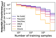

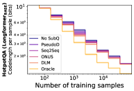

Fig. 3 shows codelengths (left) and MDL (right). For (top), decompositions consistently and significantly reduces codelength and MDL. Decomposition methods vary in how much they reduce MDL, ranked from worst to best as: no decomposition, Pseudo-Decomposition, Seq2Seq, ONUS, DLM, and oracle. Overall, the capability to answer subquestions reduces program length, especially when subquestions and their answers are of high quality.
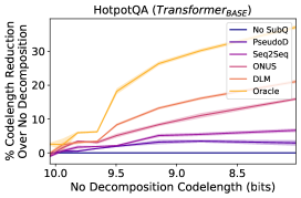
For (Fig. 3 bottom), all decomposition methods also reduce codelength and MDL, though to a lesser extent. To examine why, we plot the codelength reduction from decomposition against the original codelength for in Fig. 4 (left). As the original codelength decreases, the benefit from decomposition increases, until the no-decomposition baseline reaches a certain loss, at which point the benefit from decomposition decreases. We hypothesize that a certain, minimum amount of task understanding is necessary before decompositions are useful (see Appendix §8 for similar findings with ). However, as loss decreases, the task-relevant capabilities can be learned from the data directly, without decomposition.
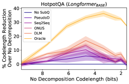


Our finding suggests that decompositions help disproportionately in the high- or mid- loss regimes rather than the low-loss regime, where QA systems are usually evaluated (i.e., when training on all examples). The limited value in low-loss regimes occurs because models approach the same, minimum loss in the limit of dataset size. Our observation partly explains why a few earlier studies (Min et al., 2019a; Chen and Durrett, 2019), which only evaluated final performance, drew the conclusion that HotpotQA does not benefit much from multi-step reasoning or question decomposition. In contrast, MDL actually does capture differences in performance across data regimes, demonstrating that RDA is the right approach going forward, especially given the growing interest in few-shot data regimes Lake et al. (2017); Brown et al. (2020)
4.2 Are Explanations and Rationales Useful?
Recent work has proposed methods that give reasons for an answer before predicting the answer to improve accuracy. Such reasons include written explanations Camburu et al. (2018); Rajani et al. (2019); Wiegreffe et al. (2020) or locating task-relevant input words Zhang et al. (2016b); Perez et al. (2019). As a testbed, these studies often use natural language inference (NLI) – checking if a premise entails or contradicts (or neither) a hypothesis. To explore if this direction is promising, we evaluate whether providing a reason is a useful capability, using NLI as a case study.
Dataset
We use the e-SNLI Camburu et al. (2018) dataset, which annotated each example in SNLI Bowman et al. (2015) with two forms of reasons: an extractive rationale that marks entailment-relevant words and a written explanation of the right answer. We randomly sample 10k examples from e-SNLI to examine the usefulness of rationales and explanations. To illustrate, e-SNLI contains an example of contradiction where the premise is “A man and a woman are dancing in the crowd.” and the hypothesis is “A man and woman dance alone.” The rationale is bolded, and the explanation is “Being in a crowd means not alone.”
Adding explanations and rationales
We view rationales and explanations as generated by a function on the input. To test if reduces MDL, we add the rationale by surrounding each entailment-relevant word with asterisks, and we add the explanation before the hypothesis, separated by a special token. For comparison, we evaluate MDL when including only the explanation as input and only the rationale patterns as input. For the latter, we use the rationale without the actual premise and hypothesis words by replacing each rationale word with “*” and other words with “_”.
Model
We use an ensemble model composed of the following model classes: FastText Bag-of-Words Joulin et al. (2017), transformers Vaswani et al. (2017) trained from scratch (110M and 340M parameter versions), (encoder-decoder; Lewis et al., 2020), (encoder-only; Lan et al., 2020), and (encoder-only; Liu et al., 2019) and the distilled version DistilRoBERTa Sanh et al. (2019), and GPT2 (decoder-only; Radford et al., 2019) and DistilGPT2 Sanh et al. (2019). For each model, we minimize cross-entropy loss and tune softmax temperature222Search over , 1k log-uniformly spaced trials. on dev to alleviate overconfidence on unseen examples Guo et al. (2017); Desai and Durrett (2020). We follow each models’ official training strategy and hyperparameter sweeps (Appendix §B.4), using the official codebase for FastText333https://github.com/facebookresearch/fastText and HuggingFace Transformers Wolf et al. (2020) with PyTorch Lightning Falcon et al. (2019) for other models.
4.2.1 Results
Fig. 4 shows codelengths (middle) and MDL (right). Adding rationales to the input greatly reduces MDL compared to using the normal input (“Input (I)”) or rationale markings without input words (“Rationale (R)”), suggesting that rationales complement the input. The reduction comes from focusing on rationale words specifically. We see almost as large MDL reductions when only including rationale-marked words and masking non-rationale words (“R Words” vs. “I+R”). In contrast, we see little improvement over rationale markings alone when using only non-rationale words with rationale words masked (“Rationale (R)” vs.“Non-R Words”). Our results show that for NLI, it is useful to first determine task-relevant words, suggesting future directions along the lines of Zhang et al. (2016b); Perez et al. (2019).
Similarly, explanations greatly reduce MDL (Fig. 4 right, rightmost two bars), especially when the input is also provided. This finding shows that explanations, like rationales, are also complementary to the input. Interestingly, adding rationales to the input reduces MDL more than adding explanations, suggesting that while explanations are useful, they are harder to use for label compression than rationales.
4.3 Examining Text Datasets
So far, we used RDA to determine when adding input features helps reduce label description lengths. Similarly, we evaluate when removing certain features increases description length, to determine what features help achieve a small MDL. Here, we view the “original” input as having certain features missing, and we evaluate the utility of a capability that recovers the missing features to return the normal task input. If reduces the label-generating program length, then it is useful to have access to (the ablated features). To illustrate, we evaluate the usefulness of different kinds of words and of word order on the General Language Understanding Evaluation benchmark (GLUE; Wang et al., 2019), a central evaluation suite in NLP, as well as SNLI and Adversarial NLI (ANLI; Nie et al., 2020).
Datasets
GLUE consists of 9 tasks (8 classification, 1 regression).444See Appendix §A.2 for details on GLUE and Appendix §B.3 for details on regression. CoLA and SST-2 are single-sentence classification tasks. MRPC, QQP, and STS-B involve determining if two sentences are similar or paraphrases of each other. QNLI, RTE, MNLI, and WNLI are NLI tasks (we omit WNLI due to its size, 634 training examples). ANLI consists of NLI data collected in three rounds, where annotators wrote hypotheses that fooled state-of-the-art NLI models trained on data from the previous round. We consider each round as a separate dataset, to examine how NLI datasets have evolved over time, from SNLI to MNLI to ANLI1, ANLI2, and ANLI3.
Experimental Setup
Following our setup for e-SNLI (§4.2), we use the 10-model ensemble and evaluating MDL on up to 10k examples per task.
4.3.1 The usefulness of part-of-speech words
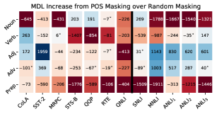
We consider the original input to be the full input with words of a certain POS masked out (with “_”) and evaluate the utility of a function that fills in the masked words. To control for the number of words masked, we restrict such that it returns a version of the input with the same proportion of words masked, chosen uniformly at random. If is useful, then words of a given type are more useful for compression than randomly-chosen input words. In particular, we report the difference between MDL when (1) words of a given POS are masked and (2) the same fraction of words are masked uniformly at random: . We evaluate nouns, verbs, adjectives, adverbs, and prepositions.555We use POS tags from spaCy’s large English model Honnibal and Montani (2017). We omit other POS, as they occur less frequently and masking them did not greatly impact MDL in preliminary experiments.
We show results in Figure 5. Adjectives are much more useful than other POS for SST-2, a sentiment analysis task where relevant terms are evidently descriptive words (e.g., “the service was terrible”). For CoLA, verbs play an important role in determining if a sentence is linguistically acceptable, likely due to the many examples evaluating verb argument structure (e.g., “The toast burned.” vs. “The toast buttered.”). Other tasks (MRPC, RTE, and QNLI) do not rely significantly on any one POS, suggesting that they require reasoning over multiple POS in tandem. Nouns are consistently less useful on NLI tasks, suggesting that NLI datasets should be supplemented with knowledge-intensive tasks like open-domain QA that rely on names and entities, in order to holistically evaluate language understanding. Prepositions are not important for any GLUE task, suggesting where GLUE can be complemented with other tasks and illustrating how RDA can be used to help form comprehensive benchmarks in the future.
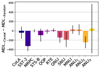
4.3.2 How useful are other word types?
Sugawara et al. (2020) hypothesized other word types that may be useful for NLP tasks. We use RDA to assess their usefulness as we did above (see Appendix §C for details). GLUE tasks vary in their reliance on “content” words. Logical words like not and every are particularly important for MNLI which involves detecting logical entailment. On the other hand, causal words (e.g., because, since, and therefore) are not particularly useful for GLUE.
4.3.3 Do Datasets Suffer from Gender Bias?
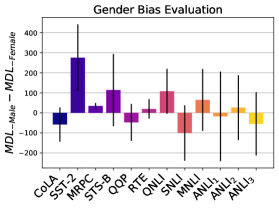
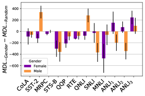
Gender bias in data is a prevalent issue in machine learning Bolukbasi et al. (2016); Blodgett et al. (2020). For example, prior work found that machine learning systems are worse at classifying images of women Phillips et al. (2000); Buolamwini and Gebru (2018), at speech recognition for women and speakers from Scotland Tatman (2017), and at POS tagging for African American vernacular Jørgensen et al. (2015). RDA can be used to diagnose such biases. Here, we do so by masking male-gendered words and evaluating the utility of an oracle function that reveals male-gendered words while masking female-gendered words. If is useful and , then masculine words are more useful than feminine words for the dataset (gender bias). We use male and female word lists from Dinan et al. (2020a, b). The two lists are similar in size (530 words each) and POS distribution (52% nouns, 29% verbs, 18% adjectives), and the male- and female- gendered words occur with similar frequency. See Appendix §C for experiments controlling for word frequency.
Fig. 6 shows the results. Masculine words are more useful for SST-2 and MRPC while no GLUE datasets have feminine words as more useful. For SST-2, feminine words occur more frequently than masculine words (2.7% vs. 2.2%, evenly distributed across class labels), suggesting that RDA uncovers a gender bias that word counts do not. This result highlights the practical value of RDA in uncovering where evaluation benchmarks under-evaluate the performance of NLP systems on text related to different demographic groups.
4.3.4 How useful is word order?
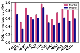
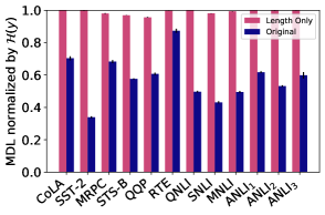
Recent work claims that state-of-the-art models do not use word order for GLUE Pham et al. (2020); Sinha et al. (2020); Gupta et al. (2021), so we use RDA to examine the utility of word order on GLUE, by testing the value of the capability to unshuffle input words when they have been shuffled.
Fig. 7 shows MDL with and without shuffling, normalized by the MDL of the label-only prior as a baseline. Word order helps to obtain smaller MDL on all tasks. For example, on MNLI, adding word order enables the labels to be compressed from of the baseline compression rate. For CoLA, the linguistic acceptability task, input word order is necessary to compress labels at all. Prior work may have come to different conclusions about the utility of word order because they evaluate the behavior of trained models on out-of-distribution (word-shuffled) text, while RDA estimates an intrinsic property of the dataset.
5 Related Work
In addition to prior work on data analysis (§1), there has been much work on model analysis (e.g., Shi et al., 2016; Alain and Bengio, 2017; Conneau et al., 2018; Jia and Liang, 2017). This line of work sometimes uses similar techniques, such as input replacement (Perez et al., 2019; Jiang and Bansal, 2019; Pham et al., 2020; Sinha et al., 2020; Gupta et al., 2021) and estimating description length (Voita and Titov, 2020; Whitney et al., 2020; Lovering et al., 2021) or other information-theoretic measures (Pimentel et al., 2020), but for a very different end: to understand how models behave and what their representations encode. While model probing can uncover characteristics of the training data (e.g., race and gender bias; Caliskan et al., 2017), models also reflect other aspects of learning Zhao et al. (2017), such as the optimization procedure, inductive bias of the model class and architecture, hyperparameters, and randomness during training. Instead of indirectly examining a dataset by probing models, we directly estimate a property intrinsic to the dataset. For further related work, see Appendix §D.
6 Conclusion
In this work, we proposed Rissanen Data Analysis (RDA), a method for examining the characteristics of a dataset. We began by viewing the labels of a dataset as being generated by a program over the inputs, then positing that a capability is helpful if it reduces the length of the shortest label-generating program. Instead of evaluating minimum program length directly, we use block-wise prequential coding to upper bound Minimum Description Length (MDL). While the choice of learning algorithm influences absolute MDL values, we only interpret MDL relative to other MDL values estimated with the same . In particular, we conduct RDA by comparing MDL with or without access to a subroutine with a certain capability, and we say that a capability is useful when invoking the subroutine reduces MDL.
We then conducted an extensive empirical analyses of various datasets with RDA. First, we showed that RDA provides intuitive results on a carefully-controlled synthetic task. Next, we used RDA to evaluate the utility of generating and answering subquestions in answering a question, finding that subquestions are indeed useful. For NLI, we found it helpful to include rationales and explanations. Finally, we showcased the general nature of RDA by applying it on a variety of other NLP tasks, uncovering the value of word order across all tasks, as well as the most useful parts of speech for different tasks, among other things. Our work opens up ample opportunity for future work: automatically uncovering dataset biases when writing data statements Gebru et al. (2018); Bender and Friedman (2018), selecting the datasets to include in future benchmarks, discovering which capabilities are helpful for different tasks, and also expanding on RDA itself, e.g., by investigating the underlying data distribution rather than a particular dataset Whitney et al. (2020). Overall, RDA is a theoretically-justified tool that is empirically useful for examining the characteristics of a wide variety of datasets.
Acknowledgments
We thank Paul Christiano, Sam Bowman, Tim Dettmers, Alex Warstadt, Will Huang, Richard Pang, Yian Zhang, Tiago Pimentel, and Patrick Lewis for helpful feedback. We are grateful to OpenAI for providing access to GPT-3 via their API Academic Access Program. We also thank Will Whitney and Peter Hase for helpful discussions, Adina Williams for the list of gendered words, Shenglong Wang for cluster support, and Amanda Ngo for figure design help. HotpotQA is licensed under CC BY-SA 4.0. KC is partly supported by Samsung Advanced Institute of Technology (Next Generation Deep Learning: from pattern recognition to AI) and Samsung Research (Improving Deep Learning using Latent Structure). KC also thanks Naver, eBay, NVIDIA, and NSF Award 1922658 for support. EP is grateful to NSF and Open Philanthropy for fellowship support.
References
- Alain and Bengio (2017) Guillaume Alain and Yoshua Bengio. 2017. Understanding intermediate layers using linear classifier probes. In ICLR.
- Antol et al. (2015) Stanislaw Antol, Aishwarya Agrawal, Jiasen Lu, Margaret Mitchell, Dhruv Batra, C. Lawrence Zitnick, and Devi Parikh. 2015. VQA: Visual Question Answering. In ICCV.
- Baker and Kim (2004) Frank B Baker and Seock-Ho Kim. 2004. Item response theory: Parameter estimation techniques. CRC Press.
- Beltagy et al. (2020) Iz Beltagy, Matthew E. Peters, and Arman Cohan. 2020. Longformer: The long-document transformer. arXiv:2004.05150.
- Bender and Friedman (2018) Emily M. Bender and Batya Friedman. 2018. Data statements for natural language processing: Toward mitigating system bias and enabling better science. Transactions of the ACL, 6:587–604.
- Bentivogli et al. (2009) Luisa Bentivogli, Ido Dagan, Hoa Trang Dang, Danilo Giampiccolo, and Bernardo Magnini. 2009. The fifth pascal recognizing textual entailment challenge. In In Proc Text Analysis Conference (TAC’09.
- Blier and Ollivier (2018) Léonard Blier and Yann Ollivier. 2018. The description length of deep learning models. In NeurIPS, volume 31, pages 2216–2226. Curran Associates, Inc.
- Blodgett et al. (2020) Su Lin Blodgett, Solon Barocas, Hal Daumé III, and Hanna Wallach. 2020. Language (technology) is power: A critical survey of “bias” in NLP. In ACL, pages 5454–5476, Online. ACL.
- Blumer et al. (1987) Alselm Blumer, Andrzej Ehrenfeucht, David Haussler, and Manfred K. Warmuth. 1987. Occam’s razor. Inf. Process. Lett., 24(6):377–380.
- Bolukbasi et al. (2016) Tolga Bolukbasi, Kai-Wei Chang, James Y Zou, Venkatesh Saligrama, and Adam T Kalai. 2016. Man is to computer programmer as woman is to homemaker? debiasing word embeddings. In NeurIPS, volume 29, pages 4349–4357. Curran Associates, Inc.
- Bowman et al. (2015) Samuel R. Bowman, Gabor Angeli, Christopher Potts, and Christopher D. Manning. 2015. A large annotated corpus for learning natural language inference. In EMNLP, pages 632–642, Lisbon, Portugal. ACL.
- Brown et al. (2020) Tom B. Brown, Benjamin Mann, Nick Ryder, Melanie Subbiah, Jared Kaplan, Prafulla Dhariwal, Arvind Neelakantan, Pranav Shyam, Girish Sastry, Amanda Askell, Sandhini Agarwal, Ariel Herbert-Voss, Gretchen Krueger, Tom Henighan, Rewon Child, Aditya Ramesh, Daniel M. Ziegler, Jeffrey Wu, Clemens Winter, Christopher Hesse, Mark Chen, Eric Sigler, Mateusz Litwin, Scott Gray, Benjamin Chess, Jack Clark, Christopher Berner, Sam McCandlish, Alec Radford, Ilya Sutskever, and Dario Amodei. 2020. Language models are few-shot learners.
- Brunet et al. (2019) Marc-Etienne Brunet, Colleen Alkalay-Houlihan, Ashton Anderson, and Richard Zemel. 2019. Understanding the origins of bias in word embeddings. In ICML, volume 97 of PMLR, pages 803–811. PMLR.
- Buolamwini and Gebru (2018) Joy Buolamwini and Timnit Gebru. 2018. Gender shades: Intersectional accuracy disparities in commercial gender classification. In Fairness, Accountability and Transparency, volume 81 of PMLR, pages 77–91, New York, NY, USA. PMLR.
- Caliskan et al. (2017) Aylin Caliskan, Joanna J Bryson, and Arvind Narayanan. 2017. Semantics derived automatically from language corpora contain human-like biases. Science, 356(6334):183–186.
- Camburu et al. (2018) Oana-Maria Camburu, Tim Rocktäschel, Thomas Lukasiewicz, and Phil Blunsom. 2018. e-snli: Natural language inference with natural language explanations. In NeurIPS, volume 31, pages 9539–9549. Curran Associates, Inc.
- Cer et al. (2017) Daniel Cer, Mona Diab, Eneko Agirre, Iñigo Lopez-Gazpio, and Lucia Specia. 2017. SemEval-2017 task 1: Semantic textual similarity multilingual and crosslingual focused evaluation. In SemEval-2017, pages 1–14, Vancouver, Canada. ACL.
- Chen and Durrett (2019) Jifan Chen and Greg Durrett. 2019. Understanding dataset design choices for multi-hop reasoning. In NAACL, Volume 1 (Long and Short Papers), pages 4026–4032, Minneapolis, Minnesota. ACL.
- Cho et al. (2014) Kyunghyun Cho, Bart van Merriënboer, Caglar Gulcehre, Dzmitry Bahdanau, Fethi Bougares, Holger Schwenk, and Yoshua Bengio. 2014. Learning phrase representations using RNN encoder–decoder for statistical machine translation. In EMNLP, pages 1724–1734, Doha, Qatar. ACL.
- Conneau et al. (2018) Alexis Conneau, German Kruszewski, Guillaume Lample, Loïc Barrault, and Marco Baroni. 2018. What you can cram into a single $&!#* vector: Probing sentence embeddings for linguistic properties. In ACL (Volume 1: Long Papers), pages 2126–2136, Melbourne, Australia. ACL.
- Cover and Thomas (2006) Thomas M. Cover and Joy A. Thomas. 2006. Elements of Information Theory (Wiley Series in Telecommunications and Signal Processing). Wiley-Interscience, USA.
- Dawid (1984) A. P. Dawid. 1984. Present position and potential developments: Some personal views: Statistical theory: The prequential approach. Journal of the Royal Statistical Society. Series A (General), 147(2):278–292.
- Desai and Durrett (2020) Shrey Desai and Greg Durrett. 2020. Calibration of pre-trained transformers. In EMNLP, pages 295–302, Online. ACL.
- Dinan et al. (2020a) Emily Dinan, Angela Fan, Adina Williams, Jack Urbanek, Douwe Kiela, and Jason Weston. 2020a. Queens are powerful too: Mitigating gender bias in dialogue generation. In EMNLP, pages 8173–8188, Online. ACL.
- Dinan et al. (2020b) Emily Dinan, Angela Fan, Ledell Wu, Jason Weston, Douwe Kiela, and Adina Williams. 2020b. Multi-dimensional gender bias classification. In EMNLP, pages 314–331, Online. ACL.
- Dixon et al. (2018) Lucas Dixon, John Li, Jeffrey Sorensen, Nithum Thain, and Lucy Vasserman. 2018. Measuring and mitigating unintended bias in text classification. In AIES.
- Dolan and Brockett (2005) William B. Dolan and Chris Brockett. 2005. Automatically constructing a corpus of sentential paraphrases. In International Workshop on Paraphrasing (IWP2005).
- Falcon et al. (2019) William Falcon et al. 2019. Pytorch lightning. GitHub. Note: https://github.com/PyTorchLightning/pytorch-lightning.
- Gebru et al. (2018) Timnit Gebru, Jamie Morgenstern, Briana Vecchione, Jennifer Wortman Vaughan, Hanna M. Wallach, Hal Daumé III, and Kate Crawford. 2018. Datasheets for datasets. CoRR, abs/1803.09010.
- Grünwald (2004) Peter Grünwald. 2004. A tutorial introduction to the minimum description length principle. CoRR, math.ST/0406077.
- Guo et al. (2017) Chuan Guo, Geoff Pleiss, Yu Sun, and Kilian Q. Weinberger. 2017. On calibration of modern neural networks. In ICML, PMLR, page 1321–1330. JMLR.org.
- Gupta et al. (2021) Ashim Gupta, Giorgi Kvernadze, and Vivek Srikumar. 2021. Bert & family eat word salad: Experiments with text understanding.
- Gururangan et al. (2018) Suchin Gururangan, Swabha Swayamdipta, Omer Levy, Roy Schwartz, Samuel Bowman, and Noah A. Smith. 2018. Annotation artifacts in natural language inference data. In NAACL, Volume 2 (Short Papers), pages 107–112, New Orleans, Louisiana. ACL.
- Guzmán et al. (2019) Francisco Guzmán, Peng-Jen Chen, Myle Ott, Juan Pino, Guillaume Lample, Philipp Koehn, Vishrav Chaudhary, and Marc’Aurelio Ranzato. 2019. The FLORES evaluation datasets for low-resource machine translation: Nepali–English and Sinhala–English. In EMNLP, pages 6098–6111, Hong Kong, China. ACL.
- Hinton and van Camp (1993) Geoffrey E. Hinton and Drew van Camp. 1993. Keeping the neural networks simple by minimizing the description length of the weights. In COLT, COLT ’93, page 5–13, New York, NY, USA. ACL.
- Holtzman et al. (2020) Ari Holtzman, Jan Buys, Li Du, Maxwell Forbes, and Yejin Choi. 2020. The curious case of neural text degeneration. In ICLR.
- Honnibal and Montani (2017) Matthew Honnibal and Ines Montani. 2017. spaCy 2: Natural language understanding with Bloom embeddings, convolutional neural networks and incremental parsing. To appear.
- Hopkins and May (2013) Mark Hopkins and Jonathan May. 2013. Models of translation competitions. In ACL (Volume 1: Long Papers), pages 1416–1424, Sofia, Bulgaria. ACL.
- Jia and Liang (2017) Robin Jia and Percy Liang. 2017. Adversarial examples for evaluating reading comprehension systems. In EMNLP, pages 2021–2031, Copenhagen, Denmark. ACL.
- Jiang and Bansal (2019) Yichen Jiang and Mohit Bansal. 2019. Avoiding reasoning shortcuts: Adversarial evaluation, training, and model development for multi-hop QA. In ACL, pages 2726–2736, Florence, Italy. ACL.
- Johnson et al. (2017) J. Johnson, B. Hariharan, Laurens van der Maaten, Li Fei-Fei, C. L. Zitnick, and Ross B. Girshick. 2017. Clevr: A diagnostic dataset for compositional language and elementary visual reasoning. CVPR, pages 1988–1997.
- Jørgensen et al. (2015) Anna Jørgensen, Dirk Hovy, and Anders Søgaard. 2015. Challenges of studying and processing dialects in social media. In Workshop on Noisy User-generated Text, pages 9–18, Beijing, China. ACL.
- Joulin et al. (2017) Armand Joulin, Edouard Grave, Piotr Bojanowski, and Tomas Mikolov. 2017. Bag of tricks for efficient text classification. In EACL: Volume 2, Short Papers, pages 427–431. ACL.
- Koh and Liang (2017) Pang Wei Koh and Percy Liang. 2017. Understanding black-box predictions via influence functions. In ICML, volume 70 of PMLR, pages 1885–1894, International Convention Centre, Sydney, Australia. PMLR.
- Kolmogorov (1968) Andrei Nikolaevic Kolmogorov. 1968. Three approaches to the quantitative definition of information. IJCM, 2(1-4):157–168.
- Lake et al. (2017) Brenden M. Lake, Tomer D. Ullman, Joshua B. Tenenbaum, and Samuel J. Gershman. 2017. Building machines that learn and think like people. Behavioral and Brain Sciences, 40:e253.
- Lalor et al. (2019) John P. Lalor, Hao Wu, and Hong Yu. 2019. Learning latent parameters without human response patterns: Item response theory with artificial crowds. In EMNLP, pages 4249–4259, Hong Kong, China. ACL.
- Lan et al. (2020) Zhenzhong Lan, Mingda Chen, Sebastian Goodman, Kevin Gimpel, Piyush Sharma, and Radu Soricut. 2020. Albert: A lite bert for self-supervised learning of language representations. In ICLR.
- Levesque et al. (2012) Hector J. Levesque, Ernest Davis, and Leora Morgenstern. 2012. The winograd schema challenge. In KR, KR’12, page 552–561. AAAI Press.
- Lewis et al. (2020) Mike Lewis, Yinhan Liu, Naman Goyal, Marjan Ghazvininejad, Abdelrahman Mohamed, Omer Levy, Veselin Stoyanov, and Luke Zettlemoyer. 2020. BART: Denoising sequence-to-sequence pre-training for natural language generation, translation, and comprehension. In ACL, pages 7871–7880, Online. ACL.
- Liu et al. (2019) Yinhan Liu, Myle Ott, Naman Goyal, Jingfei Du, Mandar Joshi, Danqi Chen, Omer Levy, Mike Lewis, Luke Zettlemoyer, and Veselin Stoyanov. 2019. Roberta: A robustly optimized BERT pretraining approach. CoRR, abs/1907.11692.
- Lovering et al. (2021) Charles Lovering, Rohan Jha, Tal Linzen, and Ellie Pavlick. 2021. Predicting inductive biases of pre-trained models. In ICLR.
- Martínez-Plumed et al. (2019) Fernando Martínez-Plumed, Ricardo B.C. Prudêncio, Adolfo Martínez-Usó, and José Hernández-Orallo. 2019. Item response theory in ai: Analysing machine learning classifiers at the instance level. Artificial Intelligence, 271:18 – 42.
- McCoy et al. (2019) Tom McCoy, Ellie Pavlick, and Tal Linzen. 2019. Right for the wrong reasons: Diagnosing syntactic heuristics in natural language inference. In ACL, pages 3428–3448, Florence, Italy. ACL.
- Micikevicius et al. (2018) Paulius Micikevicius, Sharan Narang, Jonah Alben, Gregory Diamos, Erich Elsen, David Garcia, Boris Ginsburg, Michael Houston, Oleksii Kuchaiev, Ganesh Venkatesh, and Hao Wu. 2018. Mixed precision training. In ICLR.
- Min et al. (2019a) Sewon Min, Eric Wallace, Sameer Singh, Matt Gardner, Hannaneh Hajishirzi, and Luke Zettlemoyer. 2019a. Compositional questions do not necessitate multi-hop reasoning. In ACL, pages 4249–4257, Florence, Italy. ACL.
- Min et al. (2019b) Sewon Min, Victor Zhong, Luke Zettlemoyer, and Hannaneh Hajishirzi. 2019b. Multi-hop reading comprehension through question decomposition and rescoring. In ACL, pages 6097–6109, Florence, Italy. ACL.
- Nie et al. (2020) Yixin Nie, Adina Williams, Emily Dinan, Mohit Bansal, Jason Weston, and Douwe Kiela. 2020. Adversarial NLI: A new benchmark for natural language understanding. In ACL, pages 4885–4901, Online. ACL.
- Papineni et al. (2002) Kishore Papineni, Salim Roukos, Todd Ward, and Wei-Jing Zhu. 2002. Bleu: a method for automatic evaluation of machine translation. In ACL, pages 311–318, Philadelphia, Pennsylvania, USA. ACL.
- Perez et al. (2019) Ethan Perez, Siddharth Karamcheti, Rob Fergus, Jason Weston, Douwe Kiela, and Kyunghyun Cho. 2019. Finding generalizable evidence by learning to convince Q&A models. In EMNLP, pages 2402–2411, Hong Kong, China. ACL.
- Perez et al. (2020) Ethan Perez, Patrick Lewis, Wen-tau Yih, Kyunghyun Cho, and Douwe Kiela. 2020. Unsupervised question decomposition for question answering. In EMNLP, pages 8864–8880, Online. ACL.
- Perez et al. (2018) Ethan Perez, Florian Strub, Harm de Vries, Vincent Dumoulin, and Aaron Courville. 2018. Film: Visual reasoning with a general conditioning layer. AAAI, 32(1).
- Pham et al. (2020) Thang M. Pham, Trung Bui, Long Mai, and Anh Nguyen. 2020. Out of order: How important is the sequential order of words in a sentence in natural language understanding tasks?
- Phillips et al. (2000) P. J. Phillips, Hyeonjoon Moon, S. A. Rizvi, and P. J. Rauss. 2000. The feret evaluation methodology for face-recognition algorithms. TPAMI, 22(10):1090–1104.
- Pimentel et al. (2020) Tiago Pimentel, Josef Valvoda, Rowan Hall Maudslay, Ran Zmigrod, Adina Williams, and Ryan Cotterell. 2020. Information-theoretic probing for linguistic structure. In ACL, pages 4609–4622, Online. ACL.
- Poliak et al. (2018) Adam Poliak, Jason Naradowsky, Aparajita Haldar, Rachel Rudinger, and Benjamin Van Durme. 2018. Hypothesis only baselines in natural language inference. In Joint Conference on Lexical and Computational Semantics, pages 180–191, New Orleans, Louisiana. ACL.
- Radford et al. (2019) Alec Radford, Jeff Wu, Rewon Child, David Luan, Dario Amodei, and Ilya Sutskever. 2019. Language models are unsupervised multitask learners.
- Raffel et al. (2020) Colin Raffel, Noam Shazeer, Adam Roberts, Katherine Lee, Sharan Narang, Michael Matena, Yanqi Zhou, Wei Li, and Peter J. Liu. 2020. Exploring the limits of transfer learning with a unified text-to-text transformer. JMLR, 21(140):1–67.
- Rajani et al. (2019) Nazneen Fatema Rajani, Bryan McCann, Caiming Xiong, and Richard Socher. 2019. Explain yourself! leveraging language models for commonsense reasoning. In ACL, pages 4932–4942, Florence, Italy. ACL.
- Rajpurkar et al. (2016) Pranav Rajpurkar, Jian Zhang, Konstantin Lopyrev, and Percy Liang. 2016. SQuAD: 100,000+ questions for machine comprehension of text. In EMNLP, pages 2383–2392, Austin, Texas. ACL.
- Rissanen (1978) J. Rissanen. 1978. Modeling by shortest data description. Automatica, 14(5):465 – 471.
- Rissanen (1984) J. Rissanen. 1984. Universal coding, information, prediction, and estimation. IEEE Transactions on Information Theory, 30(4):629–636.
- Rudinger et al. (2017) Rachel Rudinger, Chandler May, and Benjamin Van Durme. 2017. Social bias in elicited natural language inferences. In ACL Workshop on Ethics in NLP, pages 74–79, Valencia, Spain. ACL.
- Sanh et al. (2019) Victor Sanh, Lysandre Debut, Julien Chaumond, and Thomas Wolf. 2019. Distilbert, a distilled version of bert: smaller, faster, cheaper and lighter. ArXiv, abs/1910.01108.
- Shannon (1948) C. E. Shannon. 1948. A mathematical theory of communication. The Bell System Technical Journal, 27(3):379–423.
- Shi et al. (2016) Xing Shi, Inkit Padhi, and Kevin Knight. 2016. Does string-based neural MT learn source syntax? In EMNLP, pages 1526–1534, Austin, Texas. ACL.
- Sinha et al. (2020) Koustuv Sinha, Prasanna Parthasarathi, Joelle Pineau, and Adina Williams. 2020. Unnatural language inference.
- Socher et al. (2013) Richard Socher, Alex Perelygin, Jean Wu, Jason Chuang, Christopher D. Manning, Andrew Ng, and Christopher Potts. 2013. Recursive deep models for semantic compositionality over a sentiment treebank. In EMNLP, pages 1631–1642, Seattle, Washington, USA. ACL.
- Sugawara et al. (2020) Saku Sugawara, Pontus Stenetorp, Kentaro Inui, and Akiko Aizawa. 2020. Assessing the benchmarking capacity of machine reading comprehension datasets. AAAI, 34(05):8918–8927.
- Tatman (2017) Rachael Tatman. 2017. Gender and dialect bias in YouTube’s automatic captions. In ACL Workshop on Ethics in NLP, pages 53–59, Valencia, Spain. ACL.
- Tsuchiya (2018) Masatoshi Tsuchiya. 2018. Performance impact caused by hidden bias of training data for recognizing textual entailment. In LREC, Miyazaki, Japan. European Language Resources Association (ELRA).
- Vaswani et al. (2017) Ashish Vaswani, Noam Shazeer, Niki Parmar, Jakob Uszkoreit, Llion Jones, Aidan N. Gomez, Lukasz Kaiser, and Illia Polosukhin. 2017. Attention is all you need. CoRR, abs/1706.03762.
- Voita and Titov (2020) Elena Voita and Ivan Titov. 2020. Information-theoretic probing with minimum description length. In EMNLP, pages 183–196, Online. ACL.
- Wang et al. (2019) Alex Wang, Amanpreet Singh, Julian Michael, Felix Hill, Omer Levy, and Samuel R. Bowman. 2019. GLUE: A multi-task benchmark and analysis platform for natural language understanding. In ICLR.
- Warstadt et al. (2019) Alex Warstadt, Amanpreet Singh, and Samuel R. Bowman. 2019. Neural network acceptability judgments. TACL, 7:625–641.
- Whitney et al. (2020) William F. Whitney, Min Jae Song, David Brandfonbrener, Jaan Altosaar, and Kyunghyun Cho. 2020. Evaluating representations by the complexity of learning low-loss predictors.
- Wiegreffe et al. (2020) Sarah Wiegreffe, Ana Marasovic, and Noah A. Smith. 2020. Measuring association between labels and free-text rationales.
- Williams et al. (2018) Adina Williams, Nikita Nangia, and Samuel Bowman. 2018. A broad-coverage challenge corpus for sentence understanding through inference. In NAACL, Volume 1 (Long Papers), pages 1112–1122, New Orleans, Louisiana. ACL.
- Wolf et al. (2020) Thomas Wolf, Lysandre Debut, Victor Sanh, Julien Chaumond, Clement Delangue, Anthony Moi, Pierric Cistac, Tim Rault, Remi Louf, Morgan Funtowicz, Joe Davison, Sam Shleifer, Patrick von Platen, Clara Ma, Yacine Jernite, Julien Plu, Canwen Xu, Teven Le Scao, Sylvain Gugger, Mariama Drame, Quentin Lhoest, and Alexander Rush. 2020. Transformers: State-of-the-art natural language processing. In EMNLP: System Demonstrations, pages 38–45, Online. ACL.
- Yang et al. (2018) Zhilin Yang, Peng Qi, Saizheng Zhang, Yoshua Bengio, William Cohen, Ruslan Salakhutdinov, and Christopher D. Manning. 2018. HotpotQA: A dataset for diverse, explainable multi-hop question answering. In EMNLP, pages 2369–2380, Brussels, Belgium. ACL.
- Yogatama et al. (2019) Dani Yogatama, Cyprien de Masson d’Autume, Jerome Connor, Tomás Kociský, Mike Chrzanowski, Lingpeng Kong, Angeliki Lazaridou, Wang Ling, Lei Yu, Chris Dyer, and Phil Blunsom. 2019. Learning and evaluating general linguistic intelligence. CoRR, abs/1901.11373.
- Zhang et al. (2016a) Peng Zhang, Yash Goyal, Douglas Summers-Stay, Dhruv Batra, and Devi Parikh. 2016a. Yin and Yang: Balancing and answering binary visual questions. In CVPR.
- Zhang et al. (2016b) Ye Zhang, Iain Marshall, and Byron C. Wallace. 2016b. Rationale-augmented convolutional neural networks for text classification. In EMNLP, pages 795–804, Austin, Texas. ACL.
- Zhao et al. (2017) Jieyu Zhao, Tianlu Wang, Mark Yatskar, Vicente Ordonez, and Kai-Wei Chang. 2017. Men also like shopping: Reducing gender bias amplification using corpus-level constraints. In EMNLP, pages 2979–2989, Copenhagen, Denmark. ACL.
Appendix A Task Details
A.1 CLEVR
We examine three question categories in CLEVR which have 1-2 relevant subquestions. “Integer Comparison” questions ask to compare the numbers of two kinds of objects and have two subquestions, i.e., “Are there more cubes than spheres?” where the two subquestions are “How many cubes are there?” and “How many spheres are there?” “Attribute Comparison” questions ask to compare the properties of two objects, i.e., “Is the metal object the same color as the rubber thing?”, where there are two subquestions which each ask about the property of a single object, i.e., “What color is the metal object?” and “What color is the rubber thing?” “Same Property As” questions ask whether or not one object has the same property as another object, i.e., “What material is the sphere with the same color as the rubber cylinder?”, where there is one subquestion that asks about a property of one object, i.e., “What color is the rubber cylinder?” To obtain oracle subanswers, we use ground-truth programs given by CLEVR that can be executed over a symbolic, graph-based representation of the image to answer each question. For each question category above, we evaluate the subprogram corresponding to its subquestion(s) to generate oracle subanswer(s).
A.2 GLUE
GLUE consists of 9 tasks. Two are single-sentence classification; CoLA (Corpus of Linguistic Acceptability; Warstadt et al., 2019) involves determining if a sentence is linguistically acceptable or not, while SST-2 (Stanford Sentiment Treebank 2; Socher et al., 2013) involves predicting if a sentence has positive or negative sentiment. Three tasks involve determining if two sentences are similar or paraphrases of each other: MRPC (Microsoft Research Paragraph Corpus; Dolan and Brockett, 2005), QQP (Quora Question Pairs)666data.quora.com/First-Quora-Dataset-Release-Question-Pairs, and STS-B (Semantic Textual Similarity Benchmark; Cer et al., 2017). The rest are NLI tasks: QNLI (Question NLI, derived from SQuAD; Rajpurkar et al., 2016), RTE (Recognizing Textual Entailment; Bentivogli et al., 2009), WNLI (Winograd NLI; Levesque et al., 2012), and MNLI (Multi-genre NLI; Williams et al., 2018).
Appendix B Model Training Details
| Hyperparam | Longformer | RoBERTa | BART | ALBERT | GPT2 |
| Learning Rate | {3e-5, 5e-5, 1e-4} | {1e-5, 2e-5, 3e-5} | {5e-6, 1e-5, 2e-5} | {2e-5, 3e-5, 5e-5} | {6.25e-5, 3.125e-5, 1.25e-4} |
| Batch Size | 32 | {16, 32} | {32, 128} | {32, 128} | 32 |
| Max Epochs | 6 | 10 | 10 | 3 | 3 |
| Weight Decay | 0.01 | 0.1 | 0.01 | 0.01 | 0.01 |
| Warmup Ratio | 0.06 | 0.06 | 0.06 | 0.1 | 0.002 |
| Adam | 0.999 | 0.98 | 0.98 | 0.999 | 0.999 |
| Adam | 1e-6 | 1e-6 | 1e-8 | 1e-6 | 1e-8 |
| Grad. Clip Norm | 1 | 1 |
B.1 Distilled Language Model
B.1.1 Language Model Decompositions
Large language models (LMs) are highly effective at text generation Brown et al. (2020) but have not yet been explored in the context of question decomposition. In particular, one obstacle is the sheer computational and monetary cost associated with such models. We thus use an LM to generate question decompositions while conditioning on a few labeled question-decomposition pairs, and then we train a smaller, sequence-to-sequence model on the generated question-decomposition pairs, which we use to efficiently decompose many questions. Our approach, which we call Distilled Language Model (DLM), leverages the large LM to produce pseudo- training data for a more efficient model.
As our LM, we use the 175B parameter, pretrained GPT-3 model Brown et al. (2020) via the OpenAI API.777https://beta.openai.com/ We label the maximum number of question-decomposition pairs that fit in the context window of GPT-3 (2048 tokens or 46 question-decompositions). For labeling, we sample questions randomly from HotpotQA’s training set. To condition the LM, we format question-decomposition pairs as “[Question] = [Decomposition]”, where the decomposition consists of several consecutive subquestions. We concatenate the pairs, each on a new line, with a new question on the final line to form a prompt. We then generate from the LM, conditioned on the prompt. For decoding, we found that GPT-3 copies the question as the decomposition with greedy decoding. Therefore, we use a sample-and-rank decoding strategy, to choose the best decoding out of several possible candidates. We sample 16 decompositions with top-p sampling Holtzman et al. (2020) with , rank decompositions from highest to lowest based their average token-level log probability, and choose the highest-ranked decomposition which satisfies the basic sanity checks for decomposition from Perez et al. (2020). The sanity checks avoid the question-copying failure mode by checking if a decomposition has (1) more than one subquestion (question mark), (2) no subquestion which contains all words in the multi-hop question, and (3) no subquestion longer than the multi-hop question. We generate decompositions for HotpotQA dev questions, which we estimate costs per example or k for the 7405 dev examples via the OpenAI API. Decomposing all 90447 training examples would roughly cost an extra k, motivating distillation.
B.1.2 Distilling Decompositions
As our distilled, sequence-to-sequence model, we use the 3B parameter, pretrained T5 model Raffel et al. (2020) via HuggingFace Transformers Wolf et al. (2020). We finetune T5 on our question-decomposition examples and then use it to generate subquestions for all training questions.
To finetune T5, we split our question-decomposition examples into train (80%), dev (10%), and test (10%) splits. We finetune T5 with a learning rate of , and we sweep over label smoothing , number of training epochs , and batch size in , choosing the best hyperparmeters (, respectively) based on dev BLEU Papineni et al. (2002). We stop training early when dev BLEU does not increase after one training epoch. We generate decompositions using beam search of size and length penalty of as in Raffel et al. (2020), achieving a test BLEU of 50.7. We then finetune a new T5 model using the best hyperparameters on all question-decomposition examples except for a small set of 200 examples used for early stopping.
B.2 Longformer
Similar to Beltagy et al. (2020), we train Longformer models for up to epochs, stopping training early if dev loss doesn’t decrease after one epoch. We sweep over learning rate .
B.3 Regression
STS-B is a regression task in GLUE where labels are continuous values in . Here, we learn to minimize mean-squared error, which is equivalent to minimizing log-likelihood and thus codelength.888Cover and Thomas (2006) justifies the relationship between log-likelihood and codelength for continuous values. We treat each scalar prediction as the mean of a Gaussian distribution and tune a single standard deviation parameter shared across all predictions from a single model. We choose the variance based on dev log-likelihood using grid search over with 1000 log-uniformly spaced samples. To send the first block of labels, Alice and Bob use a uniform distribution over .
The FastText library only supports classification, so we convert STS-B to 26-way classification by rounding label values to the nearest 0.2, following Raffel et al. (2020). We compute a mean prediction by evaluating the average class label value when marginalizing over class probabilities. We then tune variance on dev as usual.


B.4 Ensemble Model
B.4.1 FastText
For the FastText classifier, we initialize with the 2M pretrained, 300-dimensional word vectors trained on Common Crawl (600B tokens).999https://fasttext.cc/docs/en/english-vectors.html We tune hyperparameters using the official implementation of automatic hyperparameter tuning, which we run for 2 hours, which is generally sufficient for hyperparmeter trials and convergence on dev accuracy. The tuning implementation chooses the hyperparameters based on dev accuracy instead of loss as we typically do, but our procedure of tuning a softmax temperature parameter helps FastText reach significantly below-baseline loss.
B.4.2 Transformer Models
The remaining models in our ensemble are transformer-based models trained with HuggingFace Transformers Wolf et al. (2020). Table 1 shows the hyperparameter ranges used for each model, which we chose based on those used in each model’s original paper for GLUE. For Transformer models trained from scratch on e-SNLI and GLUE, we use the and architecture with the RoBERTahyperparameters, except that we use a larger batch size () for the LARGE transformer, which gave better results.
B.5 Training Hardware
We train FastText on 1 CPU core (40GB of memory) and FiLM on GeForce GTX 1080ti 11GB GPUs (10GB CPU memory). We train other models with “almost floating point 16” mixed precision Micikevicius et al. (2018) on 1 RTX-8000 48GB GPU (CPU memory of 100GB for HotpotQA and 30GB for e-SNLI and GLUE).
Appendix C Additional Experiments
C.1 Is it helpful to answer subquestions?
In §4.1, we found that decompositions increase in usefulness as the original, no-decomposition model’s loss decreases, up until some point after which decompositions decrease in usefulness. To examine if the same trend holds for other models, we show the same plot for in Fig. 9. Here, decompositions increase in usefulness as the codelength (loss) of the original model decreases. However, for most decomposition methods, we do not find a point at which decompositions begin to decrease in usefulness, which we fits our hypothesis that the model must have enough data to learn the task directly in order for decompositions to become less useful. However, the slope of improvement decreases (i.e., the second derivative is negative), suggesting that, given more training data, decompositions will also peak in usefulness for .
C.2 Examining Text Datasets
How useful are content words?
Sugawara et al. (2020) hypothesized that “content” words are particularly useful for NLP tasks, taking content words to be nouns, verbs, adjectives, adverbs, or numbers. We test their utility on GLUE, SNLI, and ANLI using RDA, by evaluating (Fig. 8 left). The value is positive for SST-2, STS-B, QNLI, SNLI, and ANLI2 and negative for MRPC, MNLI, ANLI1, and ANLI3. In particular, the value for SST-2 is very high (1732), indicating that content words are important for sentiment classification, likely due to the importance of adjectives as found in §4.3.1. For QNLI, content words are important, despite earlier findings that each individual POS group (nouns, verbs, adjectives, or adverbs) was not important for QNLI (§4.3.1 Fig. 5), indicating that QNLI requires reasoning over multiple POS in tandem.
How useful are “logical” words?
Sugawara et al. (2020) hypothesized that words that have to do with the logical meaning of a sentence (e.g., quantifiers and logical connectives) are useful for NLP tasks. Using GLUE, SNLI, and ANLI, we test the usefulness of logical words, which we take as: all, any, each, every, few, if, more, most, no, nor, not, n’t, other, same, some, and than (following Sugawara et al., 2020). As shown in Fig. 8 (middle), is positive for CoLA, SST-2, MNLI, ANLI2, and ANLI3 and negative for STS-B and QQP. Notably, is large for MNLI, ANLI2, and ANLI3, three entailment detection tasks, where we expect logical words to be important.
How useful are causal words?
Another group of words that Sugawara et al. (2020) hypothesized are useful are words that express causal relationships: as, because, cause, reason, since, therefore, and why. As shown in Fig. 8 (right), to be within std. error of 0 for all tasks except SST-2, QNLI, SNLI, and ANLI2, where . Thus, causal words do not appear particularly useful for GLUE.
Do datasets suffer from gender bias, even when controlling for word frequency?
In §4.3.3, we assessed if datasets rely more on male- or female- gendered words by comparing MDL when masculine vs. feminine input words are masked, looking at . However, we may wish to focus on gender bias present in datasets beyond easy-to-detect differences in male- and female- gendered word frequency. To control for frequency, we evaluate and , as we did for our word type experiments. We show results in Fig. 10. For SST-2 and QNLI, masculine words are more useful than randomly-chosen words, while feminine words are less useful than randomly-chosen words, a sign of gender bias. Most tasks, however, do not show similar patterns of bias as SST-2 and QNLI do.
How useful is input length?
Input text length can be highly predictive of the class label (see, e.g., Dixon et al., 2018). RDA can be used to evaluate text datasets for such length bias. We evaluate MDL when only providing the input length, in terms of number of tokens (counted via spaCy).101010Masking all input tokens gave similar results. As shown in Fig. 11, the labels in MRPC, STS-B, QQP, and SNLI can be compressed using the input length, though not to a large extent. Other tasks cannot be compressed using length alone. Our results on SNLI agree with Gururangan et al. (2018) who found that hypotheses were generally shorter for entailment examples and longer for neutral examples. Similarly, they also found that length is less discriminative on MNLI compared to SNLI.
Appendix D Additional Related Work
Recent work has raised increasing awareness of the importance of characterizing the datasets we release, via datasheets Gebru et al. (2018) or data statements Bender and Friedman (2018). A key motivation for datasheets is to inform machine learning practitioners of (1) biases that models may learn when trained on the data or (2) model weaknesses that may not be caught by testing on biased data. As we saw earlier, RDA is a useful tool for catching such biases (e.g., gender bias) and thus for writing datasheets.
RDA shares high-level motivation with other data analysis methods that aim to measure intrinsic properties of the data. For example, on NLI, Gururangan et al. (2018) measure the point-wise mutual information (PMI) between the label and occurrence of different keywords to find heuristics for SNLI. Similarly, Rudinger et al. (2017) measure PMI between premise words and hypothesis words to uncover race, age, and gender stereotypes in crowdsourced SNLI hypotheses. On MNLI, McCoy et al. (2019) measure the accuracy of heuristics such as “Assume that a premise entails all hypotheses constructed from words in the premise.” These methods capture the relationship between output labels and an input feature, considered in isolation, but some features may only be useful when provided along with other features. In such cases, RDA can still capture the utility of the feature.
Other work aims to analyze properties of individual examples in a dataset. For instance, Koh and Liang (2017) use influence functions to determine which training instances are most responsible for a particular test-time prediction, e.g., for image classification. Brunet et al. (2019) use influence functions to find the training documents most responsible for producing gender-biased word embeddings. Item response theory Baker and Kim (2004) has been used to find the most challenging examples for current models Hopkins and May (2013); Lalor et al. (2019); Martínez-Plumed et al. (2019). Instead of examining individual examples, we examine general characteristics of the dataset as a whole.