Topology-driven ordering of flocking matter

Abstract

When interacting motile units self-organize into flocks, they realize one of the most robust ordered state found in nature. However, after twenty five years of intense research, the very mechanism controlling the ordering dynamics of both living and artificial flocks has remained unsettled. Here, combining active-colloid experiments, numerical simulations and analytical work, we explain how flocking liquids heal their spontaneous flows initially plagued by collections of topological defects to achieve long-ranged polar order even in two dimensions. We demonstrate that the self-similar ordering of flocking matter is ruled by a living network of domain walls linking all $\pm 1$ vortices, and guiding their annihilation dynamics. Crucially, this singular orientational structure echoes the formation of extended density patterns in the shape of interconnected bow ties. We establish that this double structure emerges from the interplay between self-advection and density gradients dressing each $-1$ topological charges with four orientation walls. We then explain how active Magnus forces link all topological charges with extended domain walls, while elastic interactions drive their attraction along the resulting filamentous network of polarization singularities. Taken together our experimental, numerical and analytical results illuminate the suppression of all flow singularities, and the emergence of pristine unidirectional order in flocking matter.

Dazzling nonequilibrium steady states are consistently observed in soft condensed matter assembled from motile units Marchetti et al. (2013); Zhang et al. (2017); Zöttl and Stark (2016); Doostmohammadi et al. (2018). But their lively dynamics comes at a high price. Unlike in equilibrium, the interplay between the inner structure and flows of active matter prohibits the emergence of macroscopic order Doostmohammadi et al. (2018); Shankar et al. (2020); Saintillan and Shelley (2012). At large scales, the sustained proliferation of topological defects traps virtually all synthetic active materials in isotropic and chaotic dynamical states. This picture of topological charges endlessly rampaging through active crystals and liquid crystals finds a remarkable exception in flocks Toner et al. (2005); Cavagna and Giardina (2014); Chaté (2020). Flocks generically refers to collections of interacting polar units collectively moving along the same average direction Toner et al. (2005) as observed over more than six orders of magnitude in scale, from kilometer-long insect swarms to colloidal and molecular flocks cruising through microfluidic devices Schaller et al. (2010); Deseigne et al. (2010); Kumar et al. (2014); Bricard et al. (2013); Yan et al. (2016). As a result of an intimate interplay between orientational and density excitations captured by Toner–Tu hydrodynamics Marchetti et al. (2013); Chaté (2020); Toner et al. (2005), both living and synthetic flocks realize one of the most stable broken symmetry phase observed in nature, in vitro and in silico: flocks can support genuine long-ranged polar order both in three and two dimensions, even when challenged by thermal fluctuations or quenched isotropic disorder Toner and Tu (1995); Chepizhko et al. (2013); Toner et al. (2018); Chardac et al. (2021); Chaté (2020). However, after twenty five years of intense research, the very mechanism controlling the ordering dynamics of flocking matter remains unsettled. The question is deceptively simple: starting from a homogeneous ensemble of motile particles undergoing uncoordinated motion, how does their velocity field initially marred by a number of topological defects heal to reach pristine orientational order, as illustrated in Supplementary Movie 1 and Fig. 1?

The response to this fundamental question remains elusive or restricted to idealized incompressible systems Mishra et al. (2010); Rana and Perlekar (2020), and the essential obstacle to elucidate the phase ordering of polar active matter lies in our poor understanding of their topological defects. Dues to the inherent coupling between polar order and density via self-propulsion, the topological defects of flocking matter are highly non linear objects yielding non-local flow distortions and extended density perturbations Kruse et al. (2004); Bricard et al. (2015); Shankar et al. (2017); Chardac et al. (2021); Chaté (2020). As a results, unlike in active nematics, or passive systems such as ferromagnets, superfluids, liquid crystals or even model universe Bray (2002); Chuang et al. (1991); Pargellis et al. (1994); Bowick et al. (1994); Ruutu et al. (1996); Shankar and Marchetti (2019); Giomi et al. (2013), the very principles ruling the interactions and annihilation of topological charges in flocks remain out of reach of our current understanding of active condensed matter.

In this article, we describe the elementary topological excitations of two dimensional flocking liquids, and elucidate their phase ordering dynamics. To do so, we first characterize the coarsening of colloidal-roller liquids after a rapid quench in the flock phase. We show that a self-similar dynamics emerges from the annihilation of $\pm 1$ vortices along a filamentous network of domain walls with no counterparts in passive materials. This lively orientational structure is mirrored by very characteristic density patterns having the shape of interconnected bow ties generic to all realizations of Toner-Tu fluids. Combining experiments, numerics and theory, we establish that this double structure is determined by extended singularity lines growing from $-1$ vortices, and shaped by the competition between self-advection and pressure gradients. Finally, we model the annihilation dynamics of vortex pairs and show how the active analogue of Magnus forces links defects of opposite topological charges with domain walls localizing all shear deformations of the spontaneously flowing liquids. In turn, orientational elasticity attract all topological defects along this emergent filamentous structure which eventually vanishes to form a material assembled from self-propelled units all flocking along the same direction.

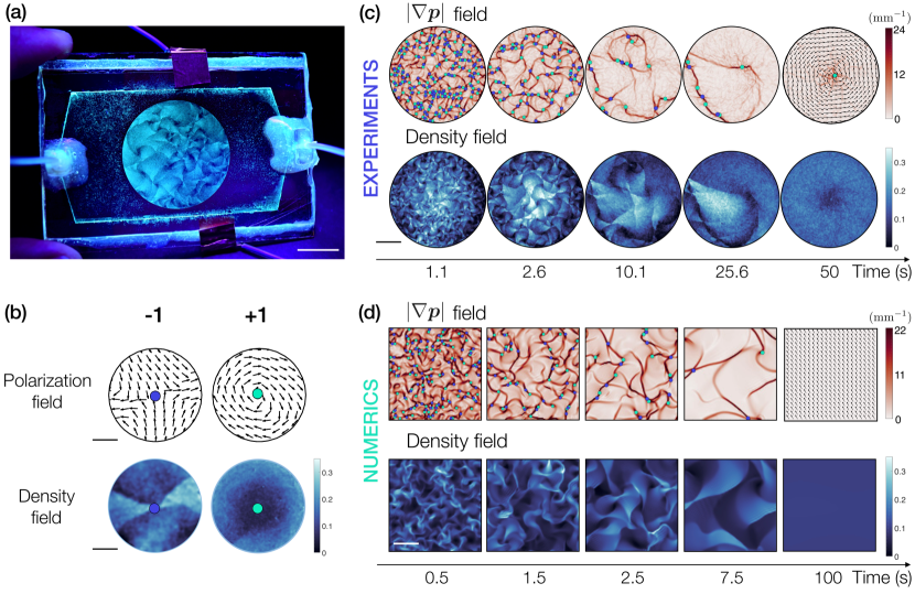
Figure 1: Ordering dynamics of flocking fluids: experiments and simulations. (a) Picture of an experiment showing $\sim 4$ millions of colloidal rollers self-assembled into an active polar fluid. The picture reveals typical bow-tie patterns prior to the formation of a pristine vortex pattern at system spanning scale, see Supplementary Movie 1. Scale bar: $1.5\,\rm cm$. (b) At the onset of flocking, the flow field of the active colloidal fluid is plagued by a collection of $\pm 1$ topological defects. The density bow ties are centered on $-1$ defects. $+1$ defects are located at the minima of the local density. The color indicates the local packing fraction. Scale bar: $250\,\rm\mu m$. (c) Series of five experimental snapshots of the density field and a map of the local stain magnitude $|\nabla\bm{p}|$. The polarization field is segmented by a fully connected network of domain walls focusing the flow distortions. Each wall coincide with a bow-tie edge in the density field. Scale bar: $2\,\rm mm$. (d) Same representation as in (c) for the numerical resolution of Toner-Tu hydrodynamics, Eqs. (1) with periodic boundary conditions, starting from a homogeneous packing fraction $\rho_{0}=0.1$ and a random velocity field. ($\lambda=0.7$, $\sigma=5\,\rm mm^{2}.s^{-2}$, $D=10^{-2}\,\rm mm^{2}.s^{-1}$, $\alpha_{0}=100\,\rm s^{-1}$, $\beta=10\,\rm mm^{-2}.s$). See Appendix B. Scale bar: $1.5\,\rm mm$.

I Colloidal flocks

To study two-dimensional flocks, we use colloidal rollers which we observe in microfluidic devices illustrated in Fig. 1(a) and Supplementary Movie 1. The experimental methods are detailed in Appendix A and Refs. Bricard et al. (2013); Geyer et al. (2018). In short, we start the experiments by filling circular microfluidic chambers of diameter comprised between $2R=3.5\,\rm mm$ and $2R=3\,\rm cm$ with inanimate polystyrene (PS) spheres of radius $a=2.4\,\rm\mu m$ in a solution of Dioctyl sulfosuccinate sodium salt (AOT) in hexadecane oil. We let the colloid sediment on the bottom electrode and adjust their area fraction to 10%. We then take advantage of the Quincke mechanism Quincke (1896); Lavrentovich (2016) to power the rotation of the PS spheres by applying a DC electric field across two transparent electrodes. Supplementary Movie 1 shows that the microscopic rollers undergo a flocking transition and collectively organize their flow into a unique system spanning vortex.

II Coarsening patterns: bow-ties and domain walls

II.1 Self-organization of a colloidal flocking liquid

To understand how colloidal rollers initially propelling along random direction self-organize to achieve nearly pristine polar order and steady flows, we measure the instantaneous density and velocity fields, ${\rho=}\rho(\bm{r},t)$ and ${\bm{v}=}\bm{v}(\bm{r},t)$, as detailed in Appendix A. We find that the spontaneous flows are first plagued by a very high density of $\pm 1$ point defects which we detect from the local winding of the polarization field: $\bm{p}=\bm{v}/|\bm{v}|$, see Fig. 1(b) and Supplemental Material. Remarkably, Fig. 1(c) and Supplementary Movie 2, showing the magnitude of the instantaneous strain field $|\nabla\bm{p}|$, both reveal that the point defects are not the sole singularities of the velocity field. In fact, they live on a fully connected network formed by persistent domain walls separating areas of incompatible orientations.

The resulting highly tortuous flows are coupled to strong density fluctuations repeating a very characteristic bow-tie pattern, giving the visual impression of a lively folded structure, even though the dynamics is strictly two dimensional, see Fig. 1(a), 1(c) and Supplementary Movie 3. This characteristic motif, emerging from a initially uniform distribution of rollers, is delimited by two discontinuity lines in the $\rho$ field which coincide with polarization walls crossing at the center of $-1$ defects, see Figs. 1(b) and 1(c). Therefore, as the defects annihilate, the number of bow ties decreases over time while their typical extent increases, until they span the whole chamber and vanish. We are then left with a heterogeneous polar fluid characterized by a stable radial density gradient, and a nearly perfect azimuthal flow around a single $+1$ defect consistently reported in flocks of motile grains Deseigne et al. (2012); Kumar et al. (2014), active biofilaments Schaller et al. (2010) and active colloids Bricard et al. (2015) in circular geometries.

II.2 Coarsening of Toner-Tu liquids

The coarsening dynamics illustrated in Fig. 1 is universal, and does not rely on any feature specific to the Quincke rollers. To demonstrate this universality, we numerically solve the Toner-Tu equations providing a hydrodynamic description of flocking fluid Toner and Tu (1995); Toner et al. (2005). They combine mass conservation and the slow dynamics of the velocity field associated to the broken rotational symmetry of the particle orientation. In its minimal form, Toner-Tu hydrodynamics reduces to:

$$\partial_{t}\rho+\nabla\cdot(\rho\bm{v})=0\;,$$ (1a)

$$\partial_{t}\bm{v}+\lambda\bm{v}\cdot\nabla\bm{v}=(\alpha-\beta v^{2})\bm{v}+D\nabla^{2}\bm{v}-\sigma\nabla\rho$$ (1b)

Eqs. (1) make the intimate relation between the density and orientational order parameter dynamics very clear. From a condensed matter perspective, Eq. (1b) can be thought as a Ginzburg-Landau theory for a broken $U(1)$ symmetry, embodied in the vector order parameter $\bm{v}$, complemented by self-convection, i.e. $\lambda\bm{v}\cdot\nabla\bm{v}$, and an ordering field $\sigma\nabla\rho$. Furthermore, mass conservation naturally couples velocity and density fluctuations. From a fluid mechanics perspective Eqs. (1) are akin to the hydrodynamics of a compressible Newtonian fluid of kinematic viscosity $D$, spontaneously flowing at average speed $v=\sqrt{\alpha/\beta}$ in response to the active drag force $(\alpha-\beta v^{2})\bm{v}$. Whereas all the coefficients in Eqs. (1) can in principle be density-dependent Geyer et al. (2018), for simplicity, we henceforth treat them as constants, with the exception of $\alpha=\alpha_{0}(\rho-\rho_{\rm c})$ and $\beta=\beta_{0}\rho$ , where $\rho_{\rm c}$ is the critical density of the flocking transition, and $\alpha_{0}$, $\beta_{0}$ are two constants. This choice guarantees a transition towards collective motion upon increasing the particle density above $\rho_{\rm c}$, as well as the saturation of the flow speed towards the speed $v_{0}=\sqrt{\alpha_{0}/\beta_{0}}$ of individual Quincke rollers when $\rho\gg\rho_{\rm c}$, deep in the ordered phase.

Using periodic boundary conditions and initializing our numerical resolution of Eqs. 1 with homogeneous density and random velocity, we find a coarsening dynamics strikingly similar to our experiments, see Fig. 1(d) and Supplementary Movies 4 and 5. The numerical methods are detailed in Appendix B. The same bow-tie patterns and domain-wall networks are consistently observed over a range of hydrodynamic parameters as detailed in Supplemental Material.

Two comments are in order. Our observations in flocking fluids are in stark contrast with the patterns found when solving the (passive) Ginzburg–Landau equation corresponding to $\lambda=\sigma=0$ in Eqs. (1), and describing for instance the relaxational dynamics of passive $XY$ ferromagnets (see e.g. Refs. Yurke et al. (1993); Bray (2002) and Supplementary Movie 6). For a passive Ginzburg–Landau dynamics, no mechanism can stabilize domain walls when a $U(1)$ symmetry is spontaneously broken. Hence, all domains walls possibly formed upon a rapid quench vanish diffusively leaving all orientational singularities at the core of $\pm 1$ pointwise vortices, see also Supplemental Material. Another noticeable difference between the defect structure of active and passive polar fluids is that $+1$ vortices in the shape of asters are present only at the very early stage of the dynamics in polar flocks, while they prevail over the full dynamics in passive Ginzburg–Landau systems.

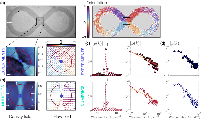
Figure 2: $-1$ topological charges are dressed with four domain walls and a density bow tie. (a) Top: Picture of a polar liquid flowing in microfluidic channel in the shape of the figure of eight and corresponding polarization field. The polarization vectors are colored according to their orientation reveal an isolated $-1$ defect. Channel width: $\rm 5\,mm$. Bottom: Polarization and density fields in the vicinity of the $-1$ defect center. The bow-tie structure is clearly visible in the absence of other defects. A single $-1$ charge is stabilized by the imposed direction of the flow field at the boundaries. The density is represented by the local packing fraction. Scale bar: $1\,\rm mm$. (b) Numerical simulation of an isolated -1 defect. Density and polarization fields. Boundary conditions described in Appendix B. Same colormaps as in (a). Scale bar: $150\,\rm\mu m$. (c) Angular power spectra of the polarization field computed along the circle showed in (a). The polarization field is not merely reduced to a single angular mode as in ideal anti-vortex with hyperbolic streamlines. Top: Experimental data. Bottom: Numerical resolution of the Toner–Tu equations Eqs. (1) in the geometry showed in (b). The solid line corresponds to the power law of the theoretical $-1$ defect geometry sketched in Fig. 3(a): four wedge-shaped regions where $\rho$ and $v$ are piecewise constant are separated by four domain walls emanating from the defect center. (d) Angular power spectra of the density field computed along the circle in (a). Same power spectra and same observation as in (c). Both $|\bm{p}(k)|$ and $|\rho(k)|$ decay algebraically revealing the singular nature of the bow tie patterns.

III Morphology of the topological defects in flocking active matter

In this section we elucidate the atypical geometry of the topological defects of flocking matter and explain how the $-1$ charges shape the emergent domain-wall network and bow-tie patterns discussed in Section II.

III.1 +1 Vortices

It is useful to recall first what determines the morphology of the $+1$ topological defects, which is clearly illustrated by the final vortex pattern of Fig. 1(c), see also Ref. Bricard et al. (2015). Mass conservation, Eq. (1a), favors exclusively the emergence of $+1$ vortices, as opposed to asters and spirals Kruse et al. (2004). They correspond to divergenceless azimuthal flows dressed with a radial density gradient extending over system spanning scales. We can understand this pattern from the stationary and long wave-length limit of Eqs. (1), where Eq. (1b) reduces to the balance between convection and density gradients, i.e.

$$\lambda\bm{v}\cdot\nabla\bm{v}+\sigma\nabla\rho=\bm{0}\;.$$ (2)

We provide a detailed solution of Eq. (2) in Appendix C. But we can readily gain some insight on the $+1$ vortex geometry by neglecting the spatial variations of the flow speed away from the defect center. This assumption is consistent with our experiments where the flow speed hardly depends on the local density sufficiently far from the defect center, see Supplemental Material. As they bend the streamlines, $+1$ defects induce a transverse centrifugal acceleration $v_{0}^{2}/r$ at a distance $r$ from the vortex center, which is balanced by a radial density gradient over the same scale: $\sigma\partial_{r}\rho=\lambda v_{0}^{2}/r$.

This competition explains why $+1$ defects are located at the minima of the $\rho$ field in Figs. 1(a) and 1(b). Moreover, it also reveals that, unlike in liquid crystals, there is no intrinsic length scale setting the size of the defect core. Both the density and flow gradients around a $+1$ vortex are determined by the system geometry as well as the position of other defects Bricard et al. (2015).

III.2 Anti-vortices, bow ties and domain walls

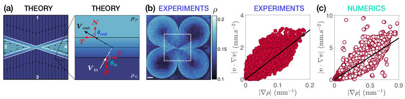
Figure 3: Bow ties and domain walls emerge from the competition between self-convection and pressure. (a). Left: Sketch of the ideal $-1$ defect configuration dressed with four domain walls. The density and flow speed are both piece-wise uniform. Right: close-up on the domain wall and definition of the local tangent $\bm{T}$ and normal $\bm{N}$ unit vectors at the domain wall separating the acute and the obtuse regions. (b). Left: Density field in a shamrock chamber. The density is represented by the local packing fraction. Scale bar: $1\,\rm mm$. Right: Measuring the stationary flow and density fields in the square region delimited in (b) left, we plot the magnitude of the convective term $|\bm{v}\cdot\nabla\bm{v}|$ against the density gradient $|\nabla\rho|$. The slope of the solid line is given by the ratio $\sigma/\lambda$ measured independently by fitting the density profiles around the $+1$ defects hosted by the circular petals, see Supplementary Information. The collapse of all data points demonstrates that density gradients locally balance the convective pressure to stabilize the singular bow-tie patterns. (c). Same measurements as in (b) for the numerical solution of Eqs. (1) in the geometry of Fig. 2(b). The straight line has a slope $\sigma/\lambda=7.1\,\rm mm^{2}\;s^{-1}$, see Appendix  B.

In contrast to the vortex flow discussed in the previous section, there exists no available characterization, or theory, for the distortions induced by a $-1$ topological charge in flocking matter. To gain insight about the structure of anti-vortices, we use a microfluidic chamber having the shape of the figure of eight showed in Fig. 2(a), such as to guarantee the existence of an isolated $-1$ topological charge in the polarization field. As prominent in Fig. 2(a), the fluid self-organizes in a “bow-tie” motif characterized by four wedge-shaped regions, where the density and velocity are spatially uniform, separated by sharp boundaries across which both fields changes discontinuously. These qualitative observations are quantitatively confirmed by the angular spectra showed in Figs. 2(b) and 2(c). They correspond respectively to experiments and numerical solutions of Eqs. (1) in the geometries showed in Fig. 2(a). In both cases, we measure the polarization field $\bm{p}$ at a distance $r$ from the vortex core and Fourier transform it with respect to the azimuthal angle $\phi$: $\bm{p}(r,\phi)=\sum_{k}\bm{p}_{k}(r)\exp(2\pi ik)$. Unlike in passive systems where the angular spectra would be solely captured by the $k=-1$ Fourier component, Fig. 2(b) reveals that a $-1$ defect excites all polarization modes in a flocking liquid. Furthermore, the algebraic decay of the two power spectra measured in experiments and simulations confirms the singular nature of the flow field. The $|\bm{p}(k)|\sim k^{-1}$ scaling, which corresponds to the Fourier transform of a piecewise constant function at large $k$ values, confirms the formation of four genuine domain walls emanating from the defect center and separating four uniform regions of incompatible orientations, see Figs. 3(a) and 2(b). The same features are observed in the azimuthal spectra of the density field, Fig. 2(c). The bow tie pattern is delimited by four density discontinuities along the four domain walls of the polarization field. We therefore conclude that the domain-wall network guiding the coarsening dynamics showed in Fig. 1 emerges from the extended singularities dressing the $-1$ topological charges of flocking matter.

III.3 Focusing the strain field and density gradients along stationary domain walls.

Our experiments and simulations demonstrate that flocking fluids do not feature perfect anti-vortices, but can support long-lived domain walls focusing all orientation and density gradients. This observation challenges our intuition based on broken $U(1)$ phases in equilibrium and begs for a quantitative explanation.

III.3.1 Flocking matter cannot host ideal anti-vortices

Let us first consider a hypothetical perfect anti-vortex having constant flow speed, $v={\rm const}$, and orientation $\bm{p}=\cos\phi\,\bm{e}_{x}-\sin\phi\,\bm{e}_{y}$, representing the far-field configuration around a classical $-1$ defect located at the origin. The associated streamlines are hyperbolas, described by the implicit equation $xy=r_{0}^{2}/2$, with $r_{0}$ the minimal distance of the streamline from the origin attained when $\phi=(\pi/4)\,n$, with $n=\pm 1,\pm 3$. In steady state, noting $\partial_{\parallel}=\bm{p}\cdot\nabla$ differentiation along a streamline, we can recast mass conservation, Eq. (1a), into

$$\frac{\partial_{\parallel}\rho}{\rho}=\frac{\cos 2\phi}{r}\;.$$ (3)

Defining the curvilinear coordinate $s$, and setting $s=0$ at $(r,\phi)=(r_{0},\pi/4)$, we can then readily integrate Eq. (3) along a streamline to express the density variations as

$$\log\left[\frac{\rho(s)}{\rho(0)}\right]=\int_{0}^{s}{\rm d}s^{\prime}\,\frac{\sqrt{r^{4}-r_{0}^{4}}}{r^{3}}\;.$$ (4)

Eq. (4) implies that the fluid density$\rho$ monotonically decreases in the upstream direction ($s<0$). However as as $v^{2}=v_{0}^{2}(1-\rho_{\rm c}/\rho)$, the flow speed decreases with $\rho$, and therefore Eq. (4) contradicts the initial assumption of a uniform flow speed. In fact, Eq. (4) implies that flocking motion would be suppressed at a sufficiently large distance from the defect center as $v$ would vanish once $\rho<\rho_{\rm c}$. We therefore conclude that macroscopic polar flocks cannot host perfect anti-vortices. The $-1$ defects of polar active matter are inherently associated to inhomogeneity in the density and flow speed. We show below how they can nevertheless be partially relieved by focusing orientational variations along one dimensional singularity lines emanating from the defect center.

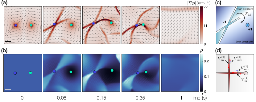
Figure 4: Self-advection and pressure gradients link topological charges with polarization walls. (a). Solving Eqs. (1) we study the dynamics of the polarization and density field around a pair of topological defects in a periodic box. At $t=0$ the flow field is the superposition of the ideal vortex and anti-vortex (hyperbolic stream lines). The flow gradient first focus to form sharp domain walls growing from the center of the $-1$ defect. The domain walls subsequently bend and rotate to link the $+1$ charge. Once the defects are linked, the $+1$ charge approaches and annihilates with the $-1$ defect, thereby yielding a perfect uniaxial order. Scale bar: $500\,\rm\mu m$. (b). Corresponding evolution of the initially uniform density field around the defect pair. A bow-tie pattern emerges as the domain walls grow and eventually vanishes once the two topological charges annihilate. Scale bar: $500\,\rm\mu m$. (c). Illustration of the pressure-driven dynamics of the domain walls around a $-1$ defect. (d). Once the four domain walls form four $\pi/2$ wedges, and link $+1$ charge, their opening remains fixed provided that the incoming and outgoing flows satisfy the horizontal mirror symmetry.

III.3.2 Strain focusing around $-1$ topological charges

To gain further physical insight on the strain focusing around $-1$ defects, we perform an additional set of experiments in the shamrock geometry showed in Fig. 3(b). The resulting flow field hosts a $-1$ defect at the shamrock’s center and one $+1$ defect in each leave. We can therefore measure the ratio $\sigma/\lambda$ by fitting the density profiles in the four vortices, as detailed in Supplementary Information. We then plot the magnitude of the convective acceleration $|\bm{v}\cdot\nabla\bm{v}|$ as a function of the modulus of the local density gradient measured in the vicinity of the defect center. Doing the same analysis for the numerical flow field of Fig. 2(b), we find that all experimental and numerical data measured around the $-1$ charge consistently obey the scaling relation $|\bm{v}\cdot\nabla\bm{v}|=(\sigma/\lambda)|\nabla\rho|$, Figs. 3(b) and 3(c). This relationship establishes that the polarization walls and density bow ties centered on $-1$ defects emerge from the competition between self-advection and density gradients generic to all spontaneously flowing liquids.

Informed by our experimental observations, we consider a piece-wise uniform configuration for $\rho$ and $\bm{p}$ in four wedge-shaped regions as defined in Fig. 3(a). To find a solution of the full active-hydrodynamic problem, we must now show that the density and flow speed can interpolate between two adjacent bulk values within finite domain walls, while the orientation $\bm{p}$ rotates, either continuously or discontinuously, by $\pi/2$. Switching again to streamline coordinates we write $\nabla=\bm{p}\,\partial_{\parallel}+\bm{p}^{\perp}\partial_{\perp}$, with $\bm{p}^{\perp}$ the counter-clockwise normal to $\bm{p}$, and Eq.  (2) takes the form

$$\bm{p}\,\partial_{\parallel}\left(\frac{1}{2}\,\lambda v^{2}+{\sigma\rho}\right)+\bm{p}^{\perp}\left({\sigma\partial_{\perp}\rho}+\kappa v^{2}\right)=\bm{0}\;,$$ (5)

where $\kappa$ is the signed curvature of the streamline. Similarly to the case of $+1$ vortices (see Sec. III.1), a transverse density gradient, $\partial_{\perp}\rho$, is necessary to counterbalance the centrifugal acceleration $\kappa v^{2}$ resulting from the bending of the streamlines. However, because of the microscopic thickness of domain walls, which sets the radius of curvature of the streamlines, such a density gradient would have to be significantly large at any finite speed $v$, thereby making the flow potentially unstable against density fluctuations. Alternatively, the fluid can continue traveling in a straight trajectory (i.e. $\kappa=0$) until reaching the domain wall centerline. The infinite curvature originating from the abrupt $\pi/2$ rotation is then compensated by a vanishing flow speed without requiring any transverse gradient ($\partial_{\perp}\rho=0$). In this case, the second term on the left-hand side of Eq. (5) vanishes, whereas the balance between self-advection and pressure gradients along the longitudinal directions results in the conservation law

$$\frac{1}{2}\,\lambda v^{2}+\sigma\rho={\rm const}\;.$$ (6)

This relation is a flocking-matter analogue of the Bernoulli law of inviscid flows. Having assumed that, deep in the ordered phase, alignment interactions ensure the local relation $v^{2}=v_{0}^{2}(1-\rho_{\rm c}/\rho)$, and using Eq.  (6) to solve Eq.  (1b) with respect to $v$, finally gives the an approximated solution for the configuration of the density and flow speed within domains walls. Calling $\rho_{<}$ and $\rho_{>}$, with $\rho_{<}\leq\rho_{>}$ and $\rho_{0}=(\rho_{<}+\rho_{>})/2$, the density of either one of the two regions separated by the same domain wall [Fig.  3(a)], we find

$$\rho(s)=\rho_{\lessgtr}+\frac{\lambda}{2\sigma}\,\left[v_{0}^{2}-v^{2}(s)\right]\;,$$ (7a)

$$v(s)=v_{0}\tanh\left(\frac{s}{\xi_{\lessgtr}}\right)\;,$$ (7b)

where we approximated $v\approx v_{0}$ away from the domain wall under the assumption that $\rho_{\lessgtr}\gg\rho_{\rm c}$. The thickness of the domain wall is given by $\xi_{\lessgtr}=\sqrt{2D/(\alpha_{0}\rho_{\lessgtr})}$, as detailed in Appendix D. This typical domain-wall solution allows the flow and density field to interpolate between seemingly incompatible domains. It further confirms that self-advection, aligning interactions and pressure gradients are the basic ingredients dressing the $-1$ topological defects with orientational domain walls and density bow ties.

However, we still need explaining the magnitude of the orientational and density discontinuities across a domain wall. Integrating the mass conservation relation in the rectangular region of arbitrary size showed in Fig. 3(a), relate the density jump to the orientation mismatch between the regions across a domain wall sketched in Figs. 3(b) and 3(c). As detailed in Appendix D, taking $\rho_{>}=2\varphi\rho_{0}$ and $\rho_{<}=2(1-\varphi)\rho_{0}$, with $1/2\leq\varphi\leq 1$, deep in the flocking phase this relation reduces to

$$\varphi=\frac{\cot\theta_{\rm in}}{\cot\theta_{\rm in}-1}=\frac{\tan\theta_{\rm out}}{\tan\theta_{\rm out}+1}\;,$$ (8)

and where $\theta_{\rm in}$ and $\theta_{\rm out}$ are the angles between the incoming and outgoing streamlines and domain wall and are such that $|\theta_{\rm in}|-|\theta_{\rm out}|=\pi/2$, see Fig. 3(a).

Toner–Tu hydrodynamics, however, cannot prescribe the absolute magnitude of the orientational discontinuity across the polarization walls, the orientation and the opening of the bow-tie pattern. Analogously to the core radius $a$ of $+1$ vortices, these three geometrical features are determined by the far-field configuration of the velocity field $\bm{v}$. They are therefore set by the boundary conditions, and interactions with the other defects populating the system, which we discuss in the next section.

IV Emergent domain-wall networks and defect interactions

We now need to explain how the polarization domain walls form the prominent network linking all $\pm 1$ defects in polar liquids when actively organizing their flows, see Figs. 1, 5 and Supplementary Movies 2 and 4.

IV.1 Interactions between domain walls and topological charges

To illuminate this spectacular example of topology-driven self-organization, we simulated the annihilation dynamics of a single pair of $\pm 1$ defects, whose initial configuration consists of a perfect vortex-anti-vortex pair in a homogeneous Toner–Tu fluid. The image sequence of Fig. 4 illustrates this three-step dynamics. Shortly after the beginning of the simulation, the $-1$ defect evolves towards the typical bow-tie structure, distinguishing two acute and two obtuse wedge-shaped regions separated by domain walls, where the velocity field rotates discontinuously by $\pi/2$. Although the neighboring $+1$ defect is initially disconnected from the four singular lines, the East-West-oriented wall subsequently bends and rotates to irreversibly connect to the $+1$ vortex center. Remarkably, it is only once the link is formed, that the $\pm 1$ charges approach one another along the polarization wall to eventually annihilate and yield a pristine uniaxial flow.

Until now our experimental and numerical findings consistently indicate that the spin-wave elasticity associated to the polarization field plays a secondary role in the emergence of the domain wall and bow tie patterns. Ignoring this contribution, $D$ term in Eq. (1b), the hydrodynamics of our active fluid is essentially that of an inviscid fluid flowing at constant speed. We can use this simplified picture to single out the mechanisms underpinning the rotation of the domain walls at the onset of a fully connected network, see Figs. 1(c) and 5(a). To do so, we consider the typical situation involving two defects of opposite charges sketched in Fig. 4(c). In the presence of a nearby $+1$ vortex the density mismatch between the acute and obtuse regions delimited by the domain walls is further increased. Therefore, the resulting pressure gradient drives a lift force that rotates the domain walls. The only possible stationary state is then given by the symmetric conformation depicted in Fig. 4(d), where the domain walls emanating from the same $-1$ defects are orthogonal and oriented at a $\pi/4$ angle with respect to the incoming and outgoing velocity field. In order to go beyond this basic symmetry argument, and account for the subsequent attraction between the defect centers, we introduce below a quantitative theory of topological defect interactions in flocking matter.

IV.2 Topological-defect interactions in flocking matter

Our minimal theory of defect interactions is inspired by the dynamics of quantized vortices in superfluids, see e.g. Ref. Sonin (1987). Given a topological defect of position $\bm{R}$ and velocity $\dot{\bm{R}}$, we show in Appendix C that convection and density gradients result in a net active Magnus force

$$\bm{F}_{\rm M}=\Gamma\,\bm{\epsilon}\cdot(\bm{V}_{\rm far}-\dot{\bm{R}})\;,$$ (9)

where $\bm{V}_{\rm far}$ is the velocity resulting from the far-field configuration of the flow, $\bm{\epsilon}$ the antisymmetric tensor, with $\epsilon_{xy}=-\epsilon_{yx}=1$ and $\epsilon_{xx}=\epsilon_{yy}=0$, and $\Gamma$ an effective drag coefficient associated with the configuration of the velocity field along the core $\mathcal{C}$, namely

$$\Gamma=\lambda\oint_{\mathcal{C}}{\rm d}{\bm{\ell}}\cdot(\rho\bm{V})\;,$$ (10)

where $\bm{V}=\bm{v}-\bm{V}_{\rm far}$ is the contribution to the total velocity originating from the defect. $\bm{F}_{\rm M}$ reflects the transverse response of the $\pm 1$ defects when driven by an external flow, and is akin to the conventional Magnus force experienced by vortices in Euler fluids Lamb (1993). In the case of an isolated defect, $\bm{F}_{\rm M}$ is either vanishing or balanced by the longitudinal drag force $\bm{F}_{\rm D}=-\zeta\dot{\bm{R}}$, with $\zeta$ a drag coefficient, resulting from the broken Galilean invariance of Eqs. (1b) and reflecting, in particular, the slow spatiotemporal variations of the order parameter $v$ originating from the motion of the defect core.

In the presence of other defects, however, both forces must balance the classic Coulomb $\bm{F}_{\rm C}$, resulting from the orientational elasticity of the polarization field $\bm{p}$ (see e.g. Ref. Chaikin and Lubensky (1995)). Under the simplifying assumption that the three forces can be computed independently, the force balance condition $\bm{F}_{\rm M}+\bm{F}_{\rm C}+\bm{F}_{\rm D}=\bm{0}$ is readily recast in an equation of motion for the interacting defect centers $\bm{R}_{i}$, with $i=1,\,2,\,3,\,\ldots$. These equations of motion read:

$$(\zeta_{i}\mathbb{1}+\Gamma_{i}\bm{\epsilon})\cdot\dot{\bm{R}}_{i}=\Gamma_{i}\bm{\epsilon}\cdot\sum_{j\neq i}\bm{V}_{j}+2\pi K_{i}\sum_{j\neq i}\Omega_{i}\Omega_{j}\frac{\bm{R}_{i}-\bm{R}_{j}}{|\bm{R}_{i}-\bm{R}_{j}|^{2}}\;,$$ (11)

where $\mathbb{1}$ is the identity tensor, $K_{i}=\zeta_{i}D$ is the orientational stiffness of the polarization field, $\Omega_{i}=\pm 1$ is the winding number of the vortices and we have approximated $\bm{V}_{\rm far}=\sum_{j\neq i}\bm{V}_{j}$. Although evidently simplified, this theory does not only shed light on the linking of topological defects by polarization walls, but also explain the subsequent annihilation of defects cruising along the resulting singularity network. Considering again the two defect configuration of Fig. 4 where two defects of opposite charge are located at $\bm{R}_{+}$ and $\bm{R}_{-}$, Eq. (11) implies that the dynamics in the direction transverse to $\bm{R}_{+}$ and $\bm{R}_{-}$ stops only when $\Gamma_{\pm}$ vanishes. In particular $\Gamma_{-}$ can be calculated from Eq. (10) in the form

$$\Gamma_{-}=\lambda\sum_{n=1}^{4}\rho{{}^{(n)}}\mathcal{L}^{(n)}\left[V_{\rm in}^{(n)}\sin\theta_{\rm in}^{(n)}+V_{\rm out}^{(n)}\sin\theta_{\rm out}^{(n)}\right]\;,$$ (12)

where the index $n$ denotes each of the four domain wall comprising the core and $\mathcal{L}^{(n)}$ their length. We find that the right-hand side of Eq. (12) vanishes in the geometry of Fig. 4(d), when the polarization walls are orthogonal and of equal length, in which case the terms in the sum have equal magnitude and alternating signs. Once this situation is reached the Magnus drag remains vanishingly small and the defect dynamics of Eq. (11) is then purely longitudinal. In other words, a remarkable prediction of our theory is that flocking liquids actively organize their flows to form polarization walls and density bow ties making the topological defect dynamics virtually indistinguishable from a passive polar materials devoid of such intricate excitations Bray (2002), see Supplementary Movies 2, 4 and 6.

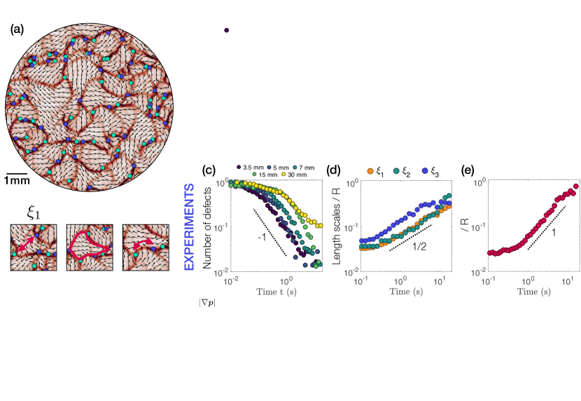
Figure 5: Orientational elasticity rules a self-similar phase ordering kinetics. (a). Snapshot of the polarization field (experiments). The red lines indicate the domain walls, the light green (resp. dark blue) circles indicate the position of the $+1$ (resp. $-1$) topological charges. The surrounding regions form domains of incompatible uniform polarization. (b). Time evolution of the total number of topological defects. We take advantage of the numerical resolution of Eqs. (1) to vary independently the three essential hydrodynamic parameters $D$, $\sigma$ and $\lambda$, setting the magnitude of the orientational elasticity, of the compressibility and of the self-advection coefficient of the flocking liquid. All the constant parameters are the same as in Fig. 1. The number of the defects plaguing the active flows decays as $1/t$ for all hydrodynamic parameters. The long-time coarsening dynamics is chiefly determined by the orientational elasticity of the polar liquid and all data collapse on a single master curve when plotted against $Dt$ (left panel inset). (c). Experimental characterization of the phase ordering kinetics in chambers of increasing size. In agreement with our simulations the number of defects decays as $1/t$. (d). Equivalently the absolute, $\xi_{1}$, and curvilinear, $\xi_{3}$, distances between the defects defined in (a) grow algebraically as $t^{1/2}$ and so does the correlation length $\xi_{2}$ of the $\bm{p}$ field, see also Supplemental Material. (e). The typical size of the polarization domains $\ell$, however, grows ballistically in time. (f). Three snapshots of the strain field corresponding to the experiment showed in (a). When a defect pair annihilates (dashed line) the domain wall emanating from them bend an eventually vanishes. As a result defects defining the vertices of the polarization network end up living along the domain walls. The typical distance between the defects hence grows slower than the distance between the network vertices $\sim\ell$.

V Self-Similar phase ordering kinetics

We are now equipped to quantitatively explain the phase ordering kinetics of flocking matter. At long time, when the defect dynamics is purely longitudinal ($\Gamma_{i}=0$), and restricted to the domain-wall network, Eq. (11) predicts an algebraic kinetics as in passive $XY$ ferromagnets and polar liquid crystals Yurke et al. (1993); Pargellis et al. (1994); Bray (2002); Jelić and Cugliandolo (2011). For instance, as defects annihilate via pair collisions, the number density of $\pm 1$ defect-pairs, $n_{\rm P}$ obeys a first order kinetic equation $\partial_{t}n_{\rm P}=-kn_{\rm P}$. Within this mean field picture, the time-dependent kinetic constant $k=k(t)$ equates the inverse annihilation time $\tau$. The latter can be estimated by solving Eq. (11) for a pair of $\pm 1$ defects in the limit of vanishing Magnus force, which yields $|\bm{R}_{+}-\bm{R}_{-}|^{2}=4\pi\tau D$. This gives $k\sim D/\delta^{2}$, with $\delta$ the typical inter-vortex distance. Finally, taking $\delta\sim 1/\sqrt{n_{\rm P}}$ gives $k\sim Dn_{\rm P}$, from which it readily follows the classic scaling law of defect coarsening of the $XY$ model and related systems: i.e. $\mathcal{N}\sim\int{\rm d}A\,n_{\rm P}\sim(Dt)^{-1}$. Equivalently, we expect the coarsening dynamics to be self-similar, and to observe a diffusive growth of all structural length scales (up to logarithmic corrections) Bray (2002).

In order to quantitatively confirm that the asymptotic phase ordering of flocks is ruled by the elasticity of this active broken symmetry phase, we first perform a series of numerical simulations varying independently the three essential parameters $\lambda$, $\sigma$ and $D$ of Toner-Tu hydrodynamics. Measuring the number of defects $\mathcal{N}$ in Fig. 5(b) unambiguously shows that the defect-annihilation kinetics is chiefly controlled by the elastic/Coulomb interactions, see also Supplemental Material. To further ascertain the self-similar nature of the dynamics, and rule out possible finite size effects, we quantify the temporal evolution of the polarization network geometry in a series of experiments and simulations spanning an order of magnitude in size. We show our experimental findings in Figs. 5(c), (d) and (e), and our consistent numerical results in Supplemental Material. Fig. 5(c) confirms that the number of $\pm 1$ topological defects decays algebraically as $\mathcal{N}\sim t^{-1}$ regardless of the system size. Equivalently, the absolute and curvilinear inter-defect distances $\xi_{1}$ and $\xi_{3}$, defined in Fig. 5(a), both obey a diffusive scaling law $\xi\sim t^{1/2}$, see Fig. 5(d). The absolute distance between the defect cores matches the orientational correlation length $\xi_{2}$ measured from the spatial decay of the two point function $C_{p}(r)=\langle\bm{p}(\bm{r},t)\cdot\bm{p}(\bm{0},t)\rangle$, which also grows diffusively in time as the colloidal flocks self-organize, see Figs. 5(d) and Supplemental Material.

However, Figs. 5(e) indicates that the size $\ell$ of the domains delimited by the polarization walls features a much faster ballistic dynamics. This observation, does not contradict our explanation of the active coarsening process, but provides an additional insight on the interplay between the domain-wall geometry and the topological charge dynamics. The faster growth of the domain size indeed originates from the fact that the $\pm 1$ defects do not only define the vertices of the network, but can also navigate along its edges. The image sequence of Fig. 5(f) illustrates this crucial aspect of the dynamics. The $\pm 1$ defects interact solely along the edges of the network and each vertex hosts a defect connected up to four defects of opposite topological charge. But, when two defects attract and annihilate the transverse domain walls they were attached to bend and connect another opposite charge, or fade away. The defect annihilation therefore leaves $\pm 1$ defects living along an edge of the network, away from a vertex. This intricate yet consistent dynamics explains why the typical domain size set by the inter-vertex distance exceeds the typical separation between opposite topological charges living along the edges.

VI Conclusion

Combining experiments, numerical simulations and analytical work, we have explained how flocks of self-propelled particles suppress the topological excitations of their flow field and self-organize in one of the most stable ordered phase observed in nature. This atypical phase ordering dynamics is ruled by the emergence of domain-wall networks shaped by self-advection and density gradient around $-1$ topological charges. This lively structure mirrored by density patterns in the form of bow-tie structures has no counterparts in passive systems. Remarkably, by actively constraining their topological charges to cruise and annihilate along polarization walls, flocking matter achieves a self-similar coarsening kinetics characterized by the same diffusive exponent as in passive ferromagnets, superconductors, or thin films of liquid crystals. The consistent and quantitative agreement between our experimental measurements and the resolution of a minimal hydrodynamic model of active polar flows further confirm the universality of our findings beyond the specifics of colloidal roller experiments.

A natural question arises from our comprehensive study: how does collective motion emerge over system spanning scales in higher dimensional systems such as bird flocks, polar tissues or 3D synthetic flocks? How does the interplay between density fluctuations and polar order alter the fundamental topological excitations of high dimensional polar active matter and compressible active liquid crystals?

Appendix A Experimental methods

A.1 Quincke rollers experiments

Our experimental setup corresponds to the one introduced in Bricard et al. (2013); Geyer et al. (2018). We disperse polystyrene colloids of radius $2.4\,\rm\mu m$ (Thermo Scientific G0500) in a solution of hexadecane including $5.5\times 10^{-2}\,\rm wt\,\%$ of dioctyl sulfosuccinate sodium salt (AOT). We then inject the suspension in microfluidic chambers made of two electrodes spaced by a $25\,\rm\mu m$-thick scotch tape. The electrodes are glass slides, coated with indium tin oxide (Solems, ITOSOL30, thickness: $80\,\rm nm$). In all our experiments, we let the colloids sediment on the bottom electrode and apply a DC voltage of $130\,\rm V$. The resulting electric field triggers the so-called Quincke electro-rotation and causes the colloids to roll at a constant speed $v_{0}=0.8\,\rm mm/s$ Bricard et al. (2013); Melcher and Taylor (1969). The geometry of the microfluidic device is illustrated in Fig. 1(a). We confine the Quincke rollers inside circular chambers of diameter comprised between $2R=3.5\,\rm mm$ and $2R=30\,\rm mm$. The confining circles are made of a $2\,\rm\mu m$-thick layer of insulating photoresist resin (Microposit S1818) patterned by means of conventional UV-Lithography as explained in Morin et al. (2017). The patterns are lithographed on the bottom electrode. We start the experiments by filling homogeneously the microfluidic chambers, and the average packing fraction $\approx 10\%$, is chosen to be far beyond the flocking transition threshold ($\approx 0.1\%$). We use the same roller fraction in all the experiments discussed in the main text.

We image the whole chambers with a Nikon AZ100 microscope using a magnification comprised between 2X and 6X depending on the chamber size, and record videos with a Luxima LUX160 camera (Ximea) at a frame rate of $200\,\rm fps$. We start measuring the flow field before the application of the DC field and stop recording only once the active flow has relaxed all its singularities, i.e. once it forms a steady vortex pattern spanning the whole circular chamber. Every experiments were repeated several times.

A.2 Velocity and density fields

In the largest chambers, we cannot detect the individual position of all the rollers with a sufficient accuracy to rely on Particle Tracking Velocimetry (PTV). Instead, we systematically use Particle Imaging Velocimetry (PIV) to construct the velocity field $\bm{v}$. PIV is performed using the PIVLab Matlab package, see Thielicke and Stamhuis (2014). The PIV-box size is $83.2\,\rm\mu m\times 83.2\,\rm\mu m$, with an overlap of a half PIV box between two adjacent measurements. We systematically checked that our findings are qualitatively insensitive to the specific choice of the PIV parameters. The polarization and strain fields are then readily computed with the same spatial resolution from $\bm{v}$.

In order to measure the density field $\rho$, we use the intensity scale of the 8-bit images. In practice, we first subtract the background image (average intensity over 500 subsequent images) to each original image, we then divide the result by its maximal intensity value. Averaging over boxes of $83.2\,\rm\mu m\times 83.2\,\rm\mu m$, we finally reconstruct the density field with the same resolution as for the velocity field. A direct comparison with measurements performed by locating the position of every single colloids using a higher magnification confirms the accuracy of our method within an accuracy of 10%.

To accurately measure the individual velocity and the packing fraction of the colloids, we track the position of all the rollers with a sub-pixel accuracy using the algorithms introduced by Lu et al. Lu et al. (2007) and by Crocker and Grier Crocker and Grier (1996). When powered with an electric field of magnitude $130\,\rm V$, all colloids roll at a constant speed: $v_{0}=0.80\pm 0.04\,\rm mm/s.$ Using the same procedure we also measure the rotational diffusivity $D_{R}$ of the rollers defined as the exponential decorrelation rate of the velocity orientation in an isotropic phase: $D_{R}=2.2\pm 0.1\,\rm s^{-1}$.

Appendix B Numerical methods

We solve numerically Eqs. (1) using an open source software package, FENICS. It offers a Finite-Element-Method (FEM) platform for solving Partial Differential Equations (PDEs), see Ref. Logg et al. (2012). We use periodic boundary conditions in a square box of size $L\times L$ for all numerical resolutions, but for the isolated $-1$ defect configuration of Figs. 2 and 3. In this case the boundary conditions are defined as follows: $\bm{p}(x=-L/2,y,t)={\bm{e}_{x}}$, $\bm{p}(x=L/2,y,t)=-{\bm{e}_{x}}$, $\bm{p}(x,y=L/2,t)={\bm{e}_{y}}$, $\bm{p}(x,y=-L/2,t)=-{\bm{e}_{y}}$. If not specified otherwise, we initialize all our numerical simulations with a homogeneous packing fraction $\rho_{0}$, and random velocity fields, and chose hydrodynamic coefficients matching the experimental values measured, and estimated in Refs. Geyer et al. (2018); Supekar et al. (2021): $\rho_{0}=0.1$, $\lambda=0.7$, $\sigma=5\,\rm mm^{2}\;s^{-2}$, $D=10^{-2}\,\rm mm^{2}\;s^{-1}$, $\alpha=\alpha_{0}(\rho-\rho_{c})$ where $\alpha_{0}=10^{2}\,\rm s^{-1}$ and $\rho_{c}=3\times 10^{-3}$, $\beta=10\,\rm mm^{-2}\;s$. All densities are normalized by $1/(\pi a^{2})$ where $a=2.4\,\rm\mu m$ is a colloid radius. $L$ is varied from $1\,\rm mm$ to $10\,\rm mm$.

The time step, between two time increments ${\delta}t$ is chosen to be small compared to the typical relaxation timescale of the fast speed mode $\tau={\alpha^{-1}(\rho_{0})}=10^{-1}\,\rm s$. In practice we take $5\times 10^{-4}\,s<\delta t\leq 5\times 10^{-3}\,s$. The computational mesh consists of $2N\times N$ triangular cells. The number of triangles per unit length is constant in all the simulations: $N=L/\delta L$, with $\delta L=0.09\,\rm mm$. The density and velocity fields are interpolated using second order polynomials on Lagrange finite element cells, see Ref. Logg et al. (2012).

Appendix C Vortex solution for $+1$ defects

In this Appendix, we provide a simple derivation of the steady-state solution of Toner-Tu equations around an isolated $+1$ defect located at the origin. Assuming that in steady state the Ginzburg-Landau term of Eq. (1b) is saturated, i.e. $v^{2}=v_{0}^{2}(1-\rho_{\rm c}/\rho)$, we seek for a vortex solution of Eq. (2) of the form $\bm{v}=v\bm{e}_{\phi}$, with $v=v(r)$ by virtue of the azimuthal symmetry of the flow ($\bm{e}_{\phi}$ indicates the azimuthal direction). With this ansatz, the velocity gradient tensor in Eq. (2) can be expressed as:

$$\nabla\bm{v}=\partial_{r}v\,\bm{e}_{r}\bm{e}_{\phi}-\frac{v}{r}\,\bm{e}_{\phi}\bm{e}_{r}\;,$$ (13)

where $\bm{e}_{r}$ is the radial unit vector. Next, replacing Eq. (13) in Eq. (2), one finds

$$r\,\partial_{r}\rho=\frac{\lambda v_{0}^{2}}{\sigma}\left(1-\frac{\rho_{\rm c}}{\rho}\right)\;,$$ (14)

whose solution can be expressed in terms of the Lambert function $W=W(z)$ defined as the solution of the transcendental equation $W\exp(W)=z$ (see e.g. Ref. Veberič (2012)), and which satisfies

$$z\,\partial_{z}W=\frac{W}{1+W}\;.$$ (15)

Setting $z=r^{\Lambda}$, $W=\rho/\rho_{\rm c}-1$ and using Eq. (15) finally yields:

$$\rho=\rho_{\rm c}\left\{1+W\left[\left(\frac{r}{a}\right)^{\Lambda}\right]\right\}\;,$$ (16a)

$$\bm{v}=v_{0}\sqrt{1-\frac{\rho}{\rho_{\rm c}}}\;\bm{e}_{\phi}\;,$$ (16b)

where $\Lambda=\lambda v_{0}^{2}/(\sigma\rho_{\rm c})$. Importantly, the integration constant $a$ represents the core radius of the vortex, namely the distance below which the order parameter is significantly lower than its preferred value: i.e. $v\ll v_{0}$. Unlike in liquid crystals, however, here there is no intrinsic length scale setting this quantity, which is then determined by the geometry of the system as well as the position of other defects Bricard et al. (2015).

Since $W(z)\approx z$, for $0\leq z\ll 1$ and $W(z)\approx\log(z)$, for $z\gg 1$, one can readily find asymptotic expansions for the density field $\rho$ in near- and far-field of the vortex, namely:

$$\rho\approx\rho_{\rm c}\left\{\begin{array}[]{lll}1+\left(\frac{r}{a}\right)^{\Lambda}&&r\approx a\\[5.0pt] 1+\Lambda\log\left(\frac{r}{a}\right)&&r\gg a\end{array}\right.\;.$$ (17)

It is worth noticing that, opposite to point vortices in inviscid fluids, whose velocity field $\bm{v}=\bm{e}_{\phi}/(2\pi r)$ monotonically decays with the distance $r$ from the center, in flocking matter the speed of a vortex increases with $r$ and eventually saturate at large distances, where $\rho\gg\rho_{\rm c}$ and $v$ reaches the maximal speed of the self-propelled units.

In practice we use Eq. (17) in Supplemental Material to measure the ratio between the two material parameters $\sigma/\lambda$.

Appendix D Boundary layer solution for $-1$ defects

The inhomogeneity in the speed of the flow around $-1$ defects cannot be entirely removed, but it can nevertheless be partially relieved by focusing density variations along extended, but narrow, domain walls emanating from the defect center and acting as interfaces between homogeneous portions of the fluid. Here, we detail the structure of the domain walls and their stabilizing effect. To do so, we construct an approximated piece-wise uniform solution of Eqs. (1). Orienting the system as illustrated in Fig. 3(a) and labeling with $\rho_{\lessgtr}$ the largest and smallest density value attained by the system, and such that $\rho_{0}=(\rho_{<}+\rho_{>})/2$, the solution takes the form:

$$(\rho,\bm{v})=\left\{\begin{array}[]{lll}(\rho_{>},\,\pm v_{>}\bm{e}_{x})&&\text{East/West}\\[5.0pt] (\rho_{<},\,\mp v_{<}\bm{e}_{y})&&\text{North/South}\;,\end{array}\right.$$ (18)

where $v_{\lessgtr}^{2}=v_{0}^{2}(1-\rho_{\rm c}/\rho_{\lessgtr})$ and East/West/North/South denotes the angular position of the four wedge-shaped regions, as displayed in Fig. 3(a). Adjacent regions have, in general, different shape, but equal area, being delimited by isosceles triangles with a common edge. Evidently, Eq. (18) is a bulk solution of Eqs.  (1), featuring a $-1$ defect at the origin.

The problem we want to solve reduces to finding the constants $\rho_{\lessgtr}$ as well as the configuration of the both fields within the domain walls. To address the first task we seek for a weak solution of Eq. (1a). The latter is obtained by expressing with

$$\hskip 12.91663pt\bm{V}_{\rm in} \hskip 2.15277pt=\hskip 2.15277ptv_{<}(\cos\theta_{\rm in}\,\bm{N}+\sin\theta_{\rm in}\,\bm{T})\;,$$ (19a)

$$\hskip 12.91663pt\bm{V}_{\rm out} =v_{>}(\cos\theta_{\rm out}\,\bm{N}+\sin\theta_{\rm out}\,\bm{T})\;,$$ (19b)

the velocity of the streamlines entering and exiting the domain wall on the basis of the normal and tangent vector, i.e. $\{\bm{N},\bm{T}\}$ [see Fig. 3(a)]. Then, assuming $\rho$ stationary and integrating both sides of Eq.  (1a) in a rectangular domain spanning a segment of the domain wall, gives

$$0=\int{\rm d}A\,\nabla\cdot(\rho\bm{v})=\rho_{<}v_{<}\cos\theta_{\rm in}+\rho_{>}v_{>}\cos\theta_{\rm out}\;.$$ (20)

Parameterizing $\rho_{>}=2\varphi\rho_{0}$ and $\rho_{<}=2(1-\varphi)\rho_{0}$, with $1/2\leq\varphi\leq 1$ and $\rho_{0}=(\rho_{<}+\rho_{>})/2$, approximating $v_{\lessgtr}\approx v_{0}$, under the assumption that $\rho_{\lessgtr}\gg\rho_{\rm c}$, and solving Eq. (20) with respect to $\varphi$, yields Eq. (8), where we made use of the fact that $|\theta_{\rm in}|-|\theta_{\rm out}|=\pi/2$.

To compute the configuration of the velocity field in the interior of the domain wall, we focus on the semi-infinite domain above the centerline of the domain wall illustrated in Fig. 3(a). Assuming Eq. (2) to hold in the interior of the domain wall, Eq. (1b) reduces to:

$$\partial_{t}\bm{v}=D\nabla^{2}\bm{v}+(\alpha-\beta v^{2})\bm{v}=0\;.$$ (21)

with boundary conditions:

$$\bm{v}(0)=\bm{0}\;,\qquad\lim_{r\rightarrow\infty}\bm{v}=\bm{V}_{\rm out}\;.$$ (22)

Now, following the discussion of Sec. III.2, we assume the streamlines to be straight, so that, in the internal upper half of the domain wall $\bm{v}$ is parallel to $\bm{V}_{\rm out}$ and its magnitude is a function of the sole arc-length distance $s$ along the streamline. Under these assumptions, using Eq. (7) and expanding Eq. (21) at the cubic order in $v/v_{>}<1$ yields

$$D\partial_{\parallel}^{2}v+(\alpha_{>}-\beta_{>}v^{2})v=0\;,$$ (23)

with the renormalized mean-field coefficients

$$\alpha_{>}=\alpha_{0}\left(\rho_{>}-\rho_{\rm c}+\frac{\lambda}{2\sigma}\,v_{>}^{2}\right)\;,$$ (24a)

$$\beta_{>}=\beta_{0}\left[\rho_{>}+\frac{\lambda}{2\sigma}\,\left(v_{0}^{2}+v_{>}^{2}\right)\right]\;.$$ (24b)

Finally, solving Eq. (23) yields

$$v=\sqrt{\frac{\alpha_{>}}{\beta_{>}}}\,\tanh\left(\frac{s}{\sqrt{2D/\alpha_{>}}}\right)\;,$$ (25)

where length scale $\sqrt{2D/\alpha_{>}}$ sets the upper half-width of the domain wall. Using the same algebraic manipulations, one can obtain an analogous approximated solution in the lower half of the domain wall, hence Eq. (7). Finally, in our experiments and, in general, away from the onset of the flocking transition, $v\approx v_{0}$, from which we obtain Eq. (7b).

Appendix E Magnus force for $\pm 1$ defects

To compute the Magnus force $\bm{F}_{\rm M}$, we assume the velocity field to be fully relaxed and Eqs. (1) can be simplified in the form

$$\partial_{t}\rho+\nabla\cdot(\rho\bm{v})=0\;,$$ (26)

$$\partial_{t}\bm{v}+\lambda\bm{v}\cdot\nabla\bm{v}+\sigma\nabla\rho=\bm{0}\;.$$ (27)

The force acting along an arbitrary contour $\mathcal{C}$ of the system, thus in particular on the boundary of the defect core, can then be expressed as

$$\bm{F}_{\rm M}=-\oint_{\mathcal{C}}{\rm d}\ell\,\bm{\Pi}\cdot\bm{N}\;,$$ (28)

where $\bm{\Pi}$ is the momentum current density defined from the equation

$$\partial_{t}(\rho\bm{v})+\nabla\cdot\bm{\Pi}=\bm{0}\;.$$ (29)

Using Eqs. (26b) one can find, after standard algebraic manipulations

$$\partial_{t}(\rho\bm{v})+\nabla\cdot\left(\frac{1}{2}\,\sigma\rho^{2}\mathbb{1}+\lambda\rho\bm{v}\bm{v}\right)=(1-\lambda)\bm{v}\partial_{t}\rho\;.$$ (30)

Now, as the motion of the core generally occurs at a much slower rate compared to the relaxation of the fields $\rho$ and $\rho\bm{v}$, one can assume all time derivatives to vanish, expect for $\dot{\bm{R}}={\rm d}\bm{R}/{\rm d}t$, with $\bm{R}$ the position of the core’s center. Using Eqs. (29) and (30) then yields

$$\bm{\Pi}=\frac{1}{2}\,\sigma\rho^{2}\mathbb{1}+\lambda\rho\bm{v}\bm{v}\;,$$ (31)

as well as

$$\Pi=\sigma\rho^{2}+\lambda\rho v^{2}={\rm const}\;,$$ (32)

where $\Pi=\mathrm{tr}(\bm{\Pi})$ and using the fact that $\rho\bm{v}$ is approximatively constant at the time scale of a moving defect. Solving Eq. (32) with respect to $\sigma\rho^{2}$, replacing this in Eq. (31) and expressing the result the in the reference frame of the moving defect, gives

$$\bm{\Pi}=\frac{1}{2}\left(\Pi-\lambda\rho|\bm{v}-\dot{\bm{R}}|^{2}\right)\mathbb{1}+\lambda\rho(\bm{v}-\dot{\bm{R}})(\bm{v}-\dot{\bm{R}})\;.$$ (33)

Dotting $\bm{\Pi}$ with the normal vector $\bm{N}$ and integrating over the contour encircling the defect core, thus yields two contributions:

$$\bm{F}_{\rm M}=\frac{1}{2}\lambda\oint_{\mathcal{C}}{\rm d}\ell\,\rho|\bm{v}-\dot{\bm{R}}|^{2}\bm{N}\\ -\lambda\oint_{\mathcal{C}}{\rm d}\ell\,\rho(\bm{v}-\dot{\bm{R}})(\bm{v}-\dot{\bm{R}})\cdot\bm{N}$$ (34)

where we assumed that $\oint_{\mathcal{C}}{\rm d}\ell\,\rho\bm{N}=\bm{0}$ because of the symmetric structure of the core. Next, expressing $\bm{v}=\bm{V}+\bm{V}_{\rm far}$, with $\bm{V}$ the contribution to the flow velocity originating from the moving defect, and $\bm{V}_{\rm far}$ any far-field contribution possibly caused by other defects, we can compute the integrals at the right-hand side of Eq. (34), which yields

$$\bm{F}_{\rm M}=\bm{\Gamma}\cdot(\bm{V}_{\rm far}-\dot{\bm{R}})\;,$$ (35)

where the effective (transverse) drag tensor takes the general form

$$\bm{\Gamma}=\lambda\oint_{\mathcal{C}}{\rm d}\ell\,\rho(\bm{V}\bm{N}-\bm{N}\bm{V})\;.$$ (36)

In deriving this equation we assumed that $\bm{V}_{\rm far}$ and $\dot{\bm{R}}$ are approximately uniform within the core and that, consistently with experimental evidence, $\oint_{\mathcal{C}}{\rm d}\ell\,\rho\bm{V}\cdot\bm{N}=0$ for both $\pm 1$ defects. Finally, expressing $\bm{V}$ in the basis $\{\bm{N},\bm{T}\}$ of the normal and vector one can explicitly calculate the integral and find $\bm{\Gamma}=\Gamma\bm{\epsilon}$, with $\Gamma$ given in Eq. (10), where ${\rm d}\bm{\ell}={\rm d}\ell\,\bm{T}$.

References

- Marchetti et al. (2013) M. C. Marchetti, J. F. Joanny, S. Ramaswamy, T. B. Liverpool, J. Prost, Madan Rao, and R. Aditi Simha, “Hydrodynamics of soft active matter,” Rev. Mod. Phys. 85, 1143–1189 (2013).
- Zhang et al. (2017) Jie Zhang, Erik Luijten, Bartosz A. Grzybowski, and Steve Granick, “Active colloids with collective mobility status and research opportunities,” Chem. Soc. Rev. 46, 5551–5569 (2017).
- Zöttl and Stark (2016) Andreas Zöttl and Holger Stark, “Emergent behavior in active colloids,” Journal of Physics: Condensed Matter 28, 253001 (2016).
- Doostmohammadi et al. (2018) Amin Doostmohammadi, Jordi Ignés-Mullol, Julia M Yeomans, and Francesc Sagués, “Active nematics,” Nature communications 9, 1–13 (2018).
- Shankar et al. (2020) Suraj Shankar, Anton Souslov, Mark J Bowick, M Cristina Marchetti, and Vincenzo Vitelli, “Topological active matter,” arXiv preprint arXiv:2010.00364 (2020).
- Saintillan and Shelley (2012) David Saintillan and Michael J Shelley, “Emergence of coherent structures and large-scale flows in motile suspensions,” Journal of the Royal Society Interface 9, 571–585 (2012).
- Toner et al. (2005) John Toner, Yuhai Tu, and Sriram Ramaswamy, “Hydrodynamics and phases of flocks,” Annals of Physics 318, 170 – 244 (2005), special Issue.
- Cavagna and Giardina (2014) Andrea Cavagna and Irene Giardina, “Bird flocks as condensed matter,” Annual Review of Condensed Matter Physics 5, 183–207 (2014).
- Chaté (2020) Hugues Chaté, “Dry aligning dilute active matter,” Annual Review of Condensed Matter Physics 11, 189–212 (2020).
- Schaller et al. (2010) Volker Schaller, Christoph Weber, Christine Semmrich, Erwin Frey, and Andreas R Bausch, “Polar patterns of driven filaments,” Nature 467, 73 (2010).
- Deseigne et al. (2010) Julien Deseigne, Olivier Dauchot, and Hugues Chaté, “Collective motion of vibrated polar disks,” Phys. Rev. Lett. 105, 098001 (2010).
- Kumar et al. (2014) Nitin Kumar, Harsh Soni, Sriram Ramaswamy, and AK Sood, “Flocking at a distance in active granular matter,” Nature Communications 5 (2014).
- Bricard et al. (2013) Antoine Bricard, Jean-Baptiste Caussin, Nicolas Desreumaux, Olivier Dauchot, and Denis Bartolo, “Emergence of macroscopic directed motion in populations of motile colloids,” Nature 503 (2013).
- Yan et al. (2016) Jing Yan, Ming Han, Jie Zhang, Cong Xu, Erik Luijten, and Steve Granick, “Reconfiguring active particles by electrostatic imbalance,” Nature materials 15, 1095–1099 (2016).
- Toner and Tu (1995) John Toner and Yuhai Tu, “Long-range order in a two-dimensional dynamical model: How birds fly together,” Phys. Rev. Lett. 75, 4326–4329 (1995).
- Chepizhko et al. (2013) Oleksandr Chepizhko, Eduardo G. Altmann, and Fernando Peruani, “Optimal noise maximizes collective motion in heterogeneous media,” Phys. Rev. Lett. 110, 238101 (2013).
- Toner et al. (2018) John Toner, Nicholas Guttenberg, and Yuhai Tu, “Swarming in the dirt: Ordered flocks with quenched disorder,” Phys. Rev. Lett. 121, 248002 (2018).
- Chardac et al. (2021) Amélie Chardac, Suraj Shankar, M. Cristina Marchetti, and Denis Bartolo, “Emergence of dynamic vortex glasses in disordered polar active fluids,” 118 (2021), 10.1073/pnas.2018218118.
- Mishra et al. (2010) Shradha Mishra, Aparna Baskaran, and M. Cristina Marchetti, “Fluctuations and pattern formation in self-propelled particles,” Phys. Rev. E 81, 061916 (2010).
- Rana and Perlekar (2020) Navdeep Rana and Prasad Perlekar, “Coarsening in the two-dimensional incompressible toner-tu equation: Signatures of turbulence,” Phys. Rev. E 102, 032617 (2020).
- Kruse et al. (2004) K. Kruse, J. F. Joanny, F. Jülicher, J. Prost, and K. Sekimoto, “Asters, vortices, and rotating spirals in active gels of polar filaments,” Phys. Rev. Lett. 92, 078101 (2004).
- Bricard et al. (2015) Antoine Bricard, Jean-Baptiste Caussin, Debasish Das, Charles Savoie, Vijayakumar Chikkadi, Kyohei Shitara, Oleksandr Chepizhko, Fernando Peruani, David Saintillan, and Denis Bartolo, “Emergent vortices in populations of colloidal rollers,” Nature communications 6, 7470 (2015).
- Shankar et al. (2017) Suraj Shankar, Mark J. Bowick, and M. Cristina Marchetti, “Topological sound and flocking on curved surfaces,” Phys. Rev. X 7, 031039 (2017).
- Bray (2002) Alan J Bray, “Theory of phase-ordering kinetics,” Advances in Physics 51, 481–587 (2002).
- Chuang et al. (1991) Isaac Chuang, Ruth Durrer, Neil Turok, and Bernard Yurke, “Cosmology in the laboratory: Defect dynamics in liquid crystals,” Science 251, 1336–1342 (1991).
- Pargellis et al. (1994) Andrew N. Pargellis, Susannah Green, and Bernard Yurke, “Planar xy-model dynamics in a nematic liquid crystal system,” Phys. Rev. E 49, 4250–4257 (1994).
- Bowick et al. (1994) Mark J Bowick, L Chandar, Eric A Schiff, and Ajit M Srivastava, “The cosmological kibble mechanism in the laboratory: string formation in liquid crystals,” Science 263, 943–945 (1994).
- Ruutu et al. (1996) VMH Ruutu, VB Eltsov, AJ Gill, TWB Kibble, M Krusius, Yu G Makhlin, B Placais, GE Volovik, and Wen Xu, “Vortex formation in neutron-irradiated superfluid 3 he as an analogue of cosmological defect formation,” Nature 382, 334–336 (1996).
- Shankar and Marchetti (2019) Suraj Shankar and M. Cristina Marchetti, “Hydrodynamics of active defects: From order to chaos to defect ordering,” Phys. Rev. X 9, 041047 (2019).
- Giomi et al. (2013) Luca Giomi, Mark J. Bowick, Xu Ma, and M. Cristina Marchetti, “Defect annihilation and proliferation in active nematics,” Phys. Rev. Lett. 110, 228101 (2013).
- Geyer et al. (2018) Delphine Geyer, Alexandre Morin, and Denis Bartolo, “Sounds and hydrodynamics of polar active fluids,” Nature materials 17, 789 (2018).
- Quincke (1896) G. Quincke, “Ueber rotationen im constanten electrischen felde,” Annalen der Physik , 417–486 (1896).
- Lavrentovich (2016) Oleg D. Lavrentovich, “Active colloids in liquid crystals,” Current Opinion in Colloid & Interface Science 21 (2016).
- Deseigne et al. (2012) Julien Deseigne, Sébastien Léonard, Olivier Dauchot, and Hugues Chaté, “Vibrated polar disks: spontaneous motion, binary collisions, and collective dynamics,” Soft Matter 8, 5629–5639 (2012).
- Yurke et al. (1993) B. Yurke, A. N. Pargellis, T. Kovacs, and D. A. Huse, “Coarsening dynamics of the xy model,” Phys. Rev. E 47, 1525–1530 (1993).
- Sonin (1987) E. B. Sonin, “Vortex oscillations and hydrodynamics of rotating superfluids,” Rev. Mod. Phys. 59, 87–155 (1987).
- Lamb (1993) Horace Lamb, Hydrodynamics (Cambridge university press, 1993).
- Chaikin and Lubensky (1995) Paul M Chaikin and Tom C Lubensky, Principles of condensed matter physics (Cambridge university press Cambridge, 1995).
- Jelić and Cugliandolo (2011) Asja Jelić and Leticia F Cugliandolo, “Quench dynamics of the 2d xy model,” Journal of Statistical Mechanics: Theory and Experiment 2011, P02032 (2011).
- Melcher and Taylor (1969) J. R. Melcher and G. I. Taylor, “Electrohydrodynamics: A review of the role of interfacial shear stresses,” Annual Review of Fluid Mechanics 1, 111–146 (1969).
- Morin et al. (2017) Alexandre Morin, Nicolas Desreumaux, Jean-Baptiste Caussin, and Denis Bartolo, “Distortion and destruction of colloidal flocks in disordered environments,” Nature Physics 13, 63 (2017).
- Thielicke and Stamhuis (2014) William Thielicke and Eize J. Stamhuis, “PIVlab – towards user-friendly, affordable and accurate digital particle image velocimetry in MATLAB,” Journal of Open Research Software 2 (2014), 10.5334/jors.bl.
- Lu et al. (2007) Peter J Lu, Peter A Sims, Hidekazu Oki, James B Macarthur, and David A Weitz, “Target-locking acquisition with real-time confocal (tarc) microscopy,” Optics express 15, 8702–8712 (2007).
- Crocker and Grier (1996) John C Crocker and David G Grier, “Methods of digital video microscopy for colloidal studies,” Journal of colloid and interface science 179, 298–310 (1996).
- Logg et al. (2012) Anders Logg, Kent-Andre Mardal, Garth N. Wells, et al., Automated Solution of Differential Equations by the Finite Element Method (Springer, 2012).
- Supekar et al. (2021) Rohit Supekar, Boya Song, Alasdair Hastewell, Alexander Mietke, and Jörn Dunkel, “Learning hydrodynamic equations for active matter from particle simulations and experiments,” arXiv preprint arXiv:2101.06568 (2021).
- Veberič (2012) Darko Veberič, “Lambert w function for applications in physics,” Computer Physics Communications 183, 2622–2628 (2012).