On single-point inversions of magnetic dipole lines in the corona

Abstract

Prompted by a recent paper by Dima and Schad, we re-consider the problem of inferring magnetic properties of the corona using polarimetric observations of magnetic dipole (M1) lines. Dima and Schad point to a potential source of degeneracy in a formalism developed by Plowman, which under some circumstances can lead to the solution being under-determined. Here we clarify the nature of the problem. Its resolution lies in solving for the scattering geometry using the elongation of the observed region of the corona. We discuss some conceptual problems that arise when casting the problem for inversion in the observer’s reference frame, and satisfactorily resolve difficulties identified by Plowman, Dima and Schad.

1 Introduction

Plowman (2014) developed a method to extract magnetic information from polarized magnetic dipole (M1) emission lines formed in the corona. In his “single point inversion” approach, the emergent polarized line profiles (measured through Stokes parameters $I,Q,U$ and $V$) are assumed to be dominated by emission from a single region along the line-of-sight (LOS) of thickness $\ell\ll R_{\odot}$, where $R_{\odot}$ is the solar radius of $7\cdot 10^{10}$ cm.

The essence of Plowman’s method is to use measured $I,Q,U$ and $V$ profiles for two M1 lines to determine components of the magnetic field within the volume defined by $\ell\cdot A$ where $A$ is the projected area of one spatial pixel of the instrument used to measure the profiles. From seven independent measurements of $I,Q,U$ and $V$ from two M1 lines ($Q$ and $U$ containing redundant information, see below), Plowman derived algebraic expressions in which seven magnetic and thermal parameters are given in terms of seven independent observables.

In a recent assessment of Plowman’s work, Dima & Schad (2020) identified a degeneracy which can cause the algebraic solutions to fail. They argued that, for many pairs of commonly used M1 lines, the algebraic solutions are formally undefined. Our purpose is to re-examine this problem.

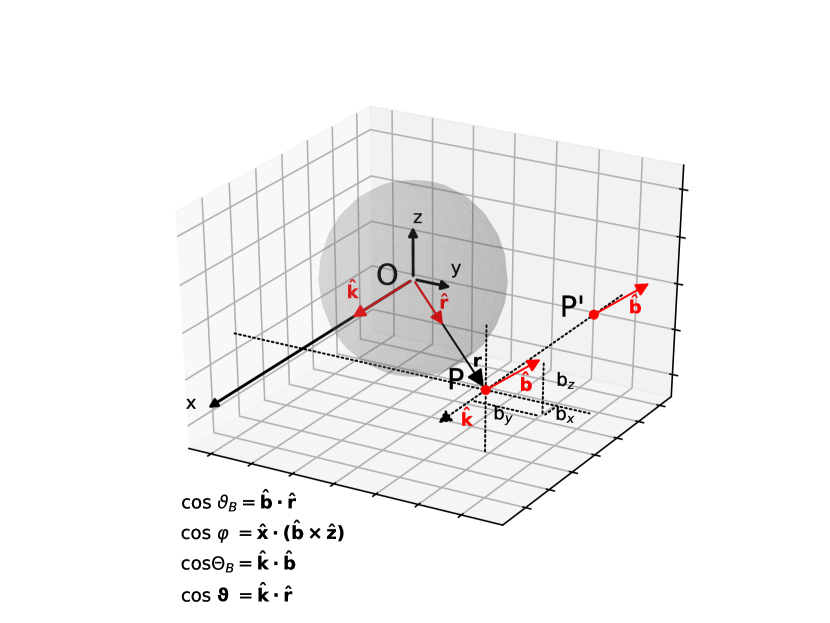
Figure 1: The scattering geometry of point $P$ is shown in the observer’s frame with projections of the magnetic field components in this frame. The line-of-sight vector lies along $\mathbf{\hat{k}}$, and the $y$ and $z$ axis are mutually orthogonal, the angle $\Phi_{B}$ ($=\gamma_{B}$ in CJ99) is defined by $\arctan\hat{b}_{y}/\hat{b}_{z}$ if we define the reference direction for linear polarization along the +ve $z-$ axis. The unit vectors of interest are marked with red arrows.

1.1 Overview of M1 line formation

In the quest to measure magnetic fields within the corona, first we must understand the origin of the emergent radiation from emitting plasma. M1 lines form in the “strong field limit” of the Hanle effect (Casini & Judge, 1999, henceforth CJ99). These lines are generally weak relative to sources of noise (e.g. Penn et al., 2004). Thus it is advantageous to integrate over the frequency-dependent line profiles, using suitable weights (the $V$ profiles are anti-symmetric around line center). Here we assume that all emission comes from a single homogeneous volume, illuminated by a spectrally flat radiation from below, along a given line of sight with length $\ell$. Then the emergent Stokes parameters are (equations 35a-35c of CJ99):

$$I = C_{JJ_{0}}\ell\,\left[1+\textstyle{\frac{1}{2\sqrt{2}}}(3\cos^{2}\!\Theta_{B}-1)\,D_{JJ_{0}}\,\sigma_{J}\right],$$ (1a)

$$Q = C_{JJ_{0}}\ell\,\,\textstyle{\frac{3}{2\sqrt{2}}}\sin^{2}\Theta_{B}\cos 2\Phi_{B}\,D_{JJ_{0}}\,\sigma_{J}\;,$$ (1b)

$$U = -C_{JJ_{0}}\ell\,\textstyle{\frac{3}{2\sqrt{2}}}\sin^{2}\Theta_{B}\sin 2\Phi_{B}\,D_{JJ_{0}}\,\sigma_{J}\;,$$ (1c)

$$V = -C_{JJ_{0}}\ell\,\frac{\omega_{B}}{\Delta\omega_{D}}\cos\Theta_{B}\left(\bar{g}_{JJ_{0}}+E_{JJ_{0}}\,\sigma_{J}\right)\;.$$ (1d)

Here, the Doppler width $\Delta\omega_{D}$ of the line arises from random thermal and other motions within $\ell\cdot A$. We assume that $\Delta\omega_{D}\gg\omega_{B}$, where $\omega_{B}$ is the Larmor frequency (CJ99). These expressions for Stokes parameters are for a M1 transition decaying from atomic level $J$ to level $J_{0}$ (here we use $J$ and $J_{0}$ to identify the unique upper and lower level of the line). The resulting frequency-integrated $I,Q,U$, and $V$ parameters depend on quantities ($D_{JJ_{0}}$, $E_{JJ_{0}}$, $\overline{g}_{JJ_{0}}$) determined by the quantum mechanics of the isolated ion, which we assume to be known. There remains six unknown parameters which contain the desired information on the plasma and magnetic field within $\ell\cdot A$.

1.2 Diagnosing the magnetized plasmas

In attempting to derive physical parameters from equations (1a)–(1d) from a set of $I,Q,U,V$ measurements, we face several challenges. In these equations the unknowns that can be solved for are $C_{JJ_{0}}$, $\ell$, $\sigma_{J}$, $\sigma_{J_{0}}$, $\omega_{B}/\Delta\omega_{D}$, $\Theta_{B}$ and $\Phi_{B}$. Two parameters can be derived directly from the observed profiles. Firstly, spectrally-resolved line profiles yield the Doppler width $\Delta\omega_{D}$. Secondly, the frequency-integrated ratio $U/Q$ immediately gives

$$\Phi_{B}=-\frac{1}{2}\arctan\frac{U}{Q}$$ (2)

Two of the five remaining parameters ($C_{JJ_{0}}$ and $\sigma_{J}$) depend on sums and differences of the populations of magnetic sub-states of level $J$. The “atomic alignment” $\sigma_{J}$ has an implicit dependence on the magnetic field geometry (CJ99, section 3.3) generated by the angle between the unit vectors $\hat{\mathbf{r}}$ from Sun center to the radiating point and $\hat{\mathbf{b}}$ (see Figure 1). This angle $\vartheta_{B}$ (with cosine $\mathbf{\hat{b}\cdot\hat{r}}$) appears only implicitly in equations (1a) to (1d) through the term $\sigma_{J}$. Clearly, $\vartheta_{B}$ varies with position $x$ along the LOS.

The three magnetic parameters that might be derived from observed Stokes parameters are related to the vector magnetic field, two angles $\Theta_{B}$ and $\Phi_{B}$ which define $\hat{\mathbf{b}}$, and $\omega_{B}$, where

$$\hbar\omega_{B}=\mu_{B}B,$$

with $\mu_{B}$ the Bohr magneton, and $B$ is the magnetic field strength. Angles $\Phi_{B}$ and $\Theta_{B}$ (equations 39a-39d of CJ99) are defined in the observer’s frame (see Figure 1). $\Phi_{B}$ is the azimuthal angle of the magnetic field vector projected on to the plane-of-sky (POS), and $\Theta_{B}$ is the angle between the line-of-sight vector $\hat{\mathbf{k}}$ and the magnetic field vector $\hat{\mathbf{b}}$.

The common factor $C_{JJ_{0}}$ is the coefficient for isotropic emission for the line intensity:

$$C_{JJ_{0}} = \frac{\hbar\omega}{4\pi}\,N_{J}A_{JJ_{0}}\;,$$ (3)

where $N_{J}$ is the population density of the upper level $J$ (i.e. the sum over all magnetic sub-states), and $A_{JJ_{0}}$ the Einstein A-coefficient. Both $N_{J}$ and $\sigma_{J}$ depend on the densities and temperatures of the plasma through collisional terms in the statistical equilibrium equations. $D_{JJ_{0}}$, and $E_{JJ_{0}}$ (Casini & Judge, 1999) depend only on $J,J_{0}$, and the effective Landé factor of the transition $J\rightarrow J_{0}$ is (Landi Degl’Innocenti & Landolfi, 2004):

$${\bar{g}_{JJ_{0}}}=\frac{1}{2}(g_{J}+g_{J_{0}})+\frac{1}{4}(g_{J}-g_{J_{0}})\left[J(J+1)-J_{0}(J_{0}+1)\right],$$ (4)

Here, $g_{J}$ and $g_{J_{0}}$ are the Landé g-factors for the splitting of levels $J$ and $J_{0}$, properties of the isolated ions assumed known from experiment and/or theory.

1.3 Plowman’s algebraic inversion

Plowman uses observations of $I,Q,U$, and $V$ from two M1 lines from the same ion of Fe¹²⁺. Along with ions of the carbon iso-electronic sequence, silicon-like Fe¹²⁺ has a ${}^{3}P_{2,1,0}$ set of ground levels between which the $J=1\rightarrow J_{0}=0$ and $J=2\rightarrow J_{0}=1$ M1 transitions occur. Anisotropic irradiation of these coronal ions by radiation from the solar surface causes $\sigma_{J}$ to be non-zero, hence leading to linear polarization (equations 1b and 1c). In using pairs of lines from the same ion, one can eliminate the need to include abundances and ionization fractions when computing $N_{J}$. In short, one has eight observed (frequency-integrated) Stokes measurements from which eight unknowns might be derived, which in principal admits algebraic solutions.

Three of these unknowns specifying the magnetic field vector ($\omega_{B},\Theta_{B},\Phi_{B})$ are common to the two lines. The Doppler width $\Delta\omega_{D}$ is readily derived from the observed line width, leaving the alignments $\sigma_{J}$, $\sigma_{J_{0}}$ and column density $N_{J}\ell$ and $N_{J_{0}}\ell$ as remaining line-dependent unknowns. We therefore have a total of seven unknowns. Further, the ratio of equations (1c) and (1b) for each line yields just one unknown from each measurement of $Q$ and $U$, independent of $I$ and $V$. The summed squares of equations (1c) and (1b) for each line yields the magnitude $L_{i}$ of the linear polarization of line $i$ through $L_{i}^{2}=Q_{i}^{2}+U_{i}^{2}$. As equation (2) applies to both lines, only seven of the observed Stokes parameters can be treated as independent measurements, these are (Plowman, 2014, section 2):

$$I_{1},L_{1},V_{1},I_{2},L_{2},V_{2},(U_{1}/Q_{1}=U_{2}/Q_{2}).$$

The essence of the method is to thus to determine the seven parameters

$$\omega_{B},\Phi_{B}\pm n{\pi/2},\Theta_{B},N_{J_{1}}\ell,\sigma_{J_{1}},N_{J_{2}}\ell,\sigma_{J_{2}},$$

algebraically from the remaining observables. If the method is applied to more than 2 lines, the problem becomes one of minimizing a goodness-of-fit instead of an algebraic solution.

2 Degeneracies

The problem identified by Dima & Schad (2020) arises when a derived atomic quantity $F_{JJ_{0}}$ is zero for both of the observed lines:

$$F_{JJ_{0}} = \sqrt{2}\frac{E_{JJ_{0}}}{D_{JJ_{0}}}-\overline{g}_{JJ_{0}}$$ (5)

$$= \frac{3}{4}\left[J(J+1)-J_{0}(J_{0}+1)-2\right](g_{J}-g_{J_{0}})$$ (6)

The latter equality applies to $\Delta J=0,\pm 1$ (Dima & Schad, 2020). In passing we note that although most M1 lines are between levels of the same (ground) term where $\Delta J=\pm 1$, there exist other M1 coronal transitions with $\Delta J=0$. For example C-, Si- and O- and S-like ions possess M1 (and E2) lines with $J=J_{0}$, for example between the $np^{2}~{}^{1}D_{2}$ and $np^{2}~{}^{3}P_{2}$ levels, $n=2,3$. A particular example is the $3p^{2}~{}^{1}D_{2}\to 3p^{2}~{}^{3}P_{2}$ transition of Si-like Fe XIII at 338.85 nm, observed during the 1965 total eclipse by Jefferies et al. (1971). Jordan (1971) reports the same transition in S-like Ni XIII at 212.6 nm, obtained during the 1970 total eclipse from a rocket spectrometer. Such transitions occur only when LS coupling breaks down, the level wavefunctions become instead mostly mixes of the two LS-coupled levels involved.

Clearly $F=0$ when $J=1,J_{0}=0$ or when $g_{J}=g_{J_{0}}$. Table 1 of Dima & Schad (2020) lists important M1 lines from the C- and Si-like isoelectronic sequences for which $F_{10}=0$ and, in LS-coupling, $g_{2}=g_{1}$.

Algebraic elimination of all unknowns except $\Theta_{B}$ from equations (1a) to (1d) yields a solution for $\sin^{2}\Theta_{B}$ in terms of the Stokes measurements and atomic parameters including $F_{i}$. To find the algebraic solutions we assume that products $D_{i}\sigma_{i}$ for both lines have the same sign (this must be the case physically unless the linear polarization is modified in a multi-level atom via other radiative or collisional transitions). In practice this assumption corresponds to the situation where the atomic alignment is determined by optical pumping of similarly anisotropic radiation through the polarizability factor $D_{i}$ for both lines. Then we find

$$\left[{\bar{g}_{1}\lambda_{1}}(I_{1}\pm L_{1})V_{2}-{\bar{g}_{2}\lambda_{2}}(I_{2}\pm L_{2})V_{1}\right]\sin^{2}\Theta_{B}$$

$$=\pm\frac{2}{3}(\lambda_{1}F_{1}L_{1}V_{2}-\lambda_{2}F_{2}L_{2}V_{1})$$ (7)

This equation differs from that of Dima & Schad (2020) by including explicitly the wavelengths $\lambda_{i}$ instead of incorporating them into a revised definition of $V$. If the term in square brackets is non-zero, two cases can be examined in terms of the atomic quantities $F_{i}$, independent of consideration of the measurements:

• $F_{1}=F_{2}=0$: The RHS is identically zero, thus the LHS of this equation is zero. Either the term in brackets [] is zero and/or $\sin^{2}\Theta_{B}=0$. If the bracketed term [] is zero, the [] term gives an equation linking all measurements $I,L,V$ of both lines, then there are fewer observables than model parameters. When [] is non-zero, this implies $\sin^{2}\Theta_{B}=0$. But when this is true, there can be no linear polarization and both $L_{i}$ must be zero no matter the measured values. Then as emphasized by Dima & Schad (2020), no solution other than $\sin^{2}\Theta_{B}=0$ is possible.

• Either of $F_{1}$ or $F_{2}$ or both are non-zero. The RHS of the equation is non-zero, so that both the bracket [] and $\sin^{2}\Theta_{B}$ are non-zero. For a given set of measurements, two solutions are possible through the $\pm L_{i}$ terms, including at least one that is physically acceptable, compatible with the reality condition $0\leq\sin^{2}\Theta_{B}\leq 1$.

The existence of solutions for $\sin^{2}\Theta_{B}$ can also be related to values of observed parameters $I_{i},L_{i},V_{i}$, for given, known non-zero values of at least one of the $F_{i}$. The $I_{i},L_{i},V_{i}$ measurements have intrinsic uncertainties, and so we must consider the statement “measurement $S_{i}=0$” to mean that the observed value, within measurement uncertainties, is compatible with zero.

• If all $V_{i}=0$ but $L_{i}\neq 0$, then, even though $\Phi_{B}$ can be defined (equation 2), $\sin^{2}\Theta_{B}$ is undetermined.

• If all $L_{i}=0$ but at least one of the $V_{i}$ are non-zero, the only solution possible is $\sin^{2}\Theta_{B}=0$, with $\Phi_{B}$ undetermined.

Both of these algebraic cases reflect the intuition that non-zero circular and linear polarization values are required to infer magnetic field properties.

We conclude that the formulation of this problem, originally based on the notion that from $N$ measurements that are independent one can derive $N$ parameters, leads to difficulties arising when naïvely applying observed values in say equation (7). Internal dependencies in the model equations (1a) to (1d) show that the observations cannot be all independent, when there are hidden symmetries. One of these symmetries found by Dima & Schad (2020) occurs when $F=0$.

3 Commentary

3.1 Incomplete formulation of the problem

When one or more of the values $F_{i}\neq 0$, Plowman’s (2014) problem recovers three magnetic variables $\Theta_{B}$, $\Phi_{B}$, $B$, and the populations $N_{J}$ and alignments $\sigma_{J}$ for each transition’s upper level $J$, from the Stokes parameters of two M1 lines. In recovering the signs of $\sigma_{J}$, a well-known ambiguity in $\Phi_{B}$ of $n\frac{\pi}{2}$ with $n$ any integer, is reduced to $n{\pi}$ (see equations (1b) and (1c)) because two of the angular quadrants for $\Phi_{B}$ are eliminated (Judge, 2007). Subject to these ambiguities, the magnetic field vector can be regarded to be known. In principle, a map of $\mathbf{B}$ in the plane-of-sky ($x=0$, say) might then be constructed. Such maps were made commonly in early coronagraphic studies of just $I,Q,U$ coronal data (Querfeld, 1977; Querfeld & Smartt, 1984; Arnaud & Newkirk, 1987).

However, we have become concerned that these algebraic solutions, written explicitly in terms of angular variables $\Theta_{B}$ and $\Phi_{B}$ defined in the observer’s frame, appear to be independent of the scattering geometry. This point can be appreciated by inspection of Figure 1. Any unit magnetic field vector fixes the values of $\Phi_{B}$ and $\Theta_{B}$ for all values of $x$ along the LOS. The only information on the $x$ coordinate in the algebraic solutions is therefore encoded only in the atomic alignments $\sigma_{J}$ and $\sigma_{J_{0}}$. The level populations $N_{J},N_{J_{0}}$ determine just the total number of emitted photons.

Suppose that we know by independent means that the bulk of the emission comes from values of $x$ where $|x|\ll R_{\odot}$, and we have in hand the solutions for the seven variables from Plowman’s method. Two questions then arise: are the alignment factors derived physically acceptable? Are they compatible with $x\approx 0$ to within uncertainties?

This thought experiment suggests that the data might be used also to constrain the coordinate $x$ of the emitting plasma. With $\Phi_{B}$ determined modulo $n\pi$ from equation (2), and $\Theta_{B}$ from a successful application of equation (7), one can imagine emission originating from different points along the $x$ axis, for fixed $y$ and $z$. The magnitudes and signs of alignments are determined in part by the value of $\cos\vartheta_{B}=\hat{\mathbf{b}}\cdot\hat{\mathbf{r}}$. Now $\hat{\mathbf{r}}$ varies according to the geometry independent of the fixed value of $\hat{\mathbf{b}}$, therefore we see that the atomic alignments implicitly contain information about the LOS coordinate $x$ of the plasma.

As originally conceived by one of us (PGJ), the method developed by Plowman tacitly assumed that the plasma emission would arise from regions where $|x|\ll R_{\odot}$. This assumption, also adopted in the earlier work (Querfeld, 1977; Querfeld & Smartt, 1984; Arnaud & Newkirk, 1987), can only be weakly justified, noting that the plasma pressure scale height $h$ $\sim 0.06R_{\odot}$ in the inner corona. Regions where $|x|\geq\sqrt{R_{\odot}h}\approx 0.25R_{\odot}$ will typically be too tenuous to contribute significantly to line emission. With this assumption, the geometry is fixed with $\cos\vartheta=\hat{\mathbf{k}}\cdot\hat{\mathbf{r}}\approx 0$. The emission lines we observe are scattered by $\vartheta\approx 90^{\circ}$ towards the observer. If we choose to accept these conditions, equations (42) and (44) of Casini & Judge (1999) read

$$\cos\Theta_{B}=\sin\theta_{B}\cos\varphi_{B}$$

and

$$\sin\Theta_{B}\cos\Phi_{B}=\cos\vartheta_{B}$$

which, given a particular solution to Plowman’s problem, are sufficient to solve for $\vartheta_{B}$ and $\varphi_{B}$ to define the geometry in the solar rest frame.

3.2 An explicit formulation

In hindsight, the inversion scheme of Plowman (2014) is seen as an incomplete determination of plasma and magnetic properties from Stokes data. In seeking the minimal set of seven parameters $N_{J},N_{J_{0}},\sigma_{J},\sigma_{J_{0}},\Theta_{B},\Phi_{B}$, and $B$ from seven independent measurements $S_{i}$, the scattering geometry is not explicitly treated. Yet we argued in the previous subsection that such information is implicitly contained in the atomic alignments.

These difficulties have prompted us to reformulate this “inversion problem”, to build a database of Stokes parameters computed from single points along the line-of-sight (Judge & Paraschiv, 2021). Stokes parameters computed within the grid are sought to match observations through a goodness-of-fit metric. The $y$-coordinate (i.e., astronomical elongation) is used as an observable, allowing us solve for $x$ values matching observation and theory. Only two dimensional searches ($x$ and $y$) are needed in the database to find the optimal solutions, because the statistical equilibrium equations for the radiating ions are invariant to rotation by an angle $\alpha$ around the $x$-axis for spherically symmetric radiation from the solar surface. Thus, the Stokes parameters $Q$ and $U$ seen by an observer can simply be rotated through an angle $-2\alpha$ prior to seeking solutions in the database’s 2D plane.

How does this explicit approach relate to that of Plowman (2014)? Both seek solutions compatible with observations, both have intrinsic ambiguities (Judge, 2007). The difference is in using the observed $y$-coordinate and a search along $x$ to fix the scattering geometry. As we show below, the redundancy problem identified by Dima & Schad (2020) then vanishes. Independent of values of $F_{JJ_{0}}$, in each identified solution, all angles in the solar reference frame are known (i.e., $\hat{\mathbf{k}}\cdot\hat{\mathbf{r}}$, $\hat{\mathbf{k}}\cdot\hat{\mathbf{b}}$, and $\hat{\mathbf{b}}\cdot\hat{\mathbf{r}}$; see Figure 1). The extra numerical work in the database approach is minimal.

3.3 $F=0$ and the explicit method

Is the “$F=0$ redundancy problem” of Dima & Schad (2020) then common to both approaches? Or, does the inclusion of the $y$-coordinate and use of alignment factors to solve for $x$ avoid this problem? The answers are no and yes respectively.

Proposition

In solving for the geometry using the additional information in the atomic alignments, the values of the $F_{i}$ play no role in the determination of $\Theta_{B}$.

Proof

Consider the geometry of Fig. 1, and make no assumptions about $F_{i}$. For simplicity assume that the unit vector $\hat{\mathbf{b}}$ of the magnetic field is fixed along any given $y_{0}$. First we demonstrate that the alignment factors are simple functions of the $x$-coordinate of the emitting volume $\ell\cdot A$.

First consider the dependence on $x$ of the angles $\vartheta,\vartheta_{B},\phi_{B}$ in the solar reference frame. $\vartheta=\arctan y_{0}/x$ is clearly a single valued function of $x$ for any $y_{0}$.

The alignment factors are indeed simple functions, when generated by unpolarized, and anisotropic but cylindrically symmetric photospheric radiation. In this case they are proportional to the anisotropy factor

$$\frac{J_{0}^{2}}{J_{0}^{0}}=\frac{1}{4\sqrt{2}}(3\cos^{2}\vartheta_{B}-1)(1+\cos\vartheta_{M})\cos\vartheta_{M},$$ (8)

where $\vartheta_{M}$ is the half-angle defining the cone of solar irradiation (this is equation (31) of Casini & Judge, 1999). The dependence of $\sigma_{J}$ on $\vartheta_{B}$ leads to the well-known Van Vleck effect (e.g., Sahal-Brechot 1977). From Figure 1 we see

$$\cos\vartheta_{B}=\hat{\mathbf{b}}\cdot\hat{\mathbf{r}}=b_{x}\,x+b_{y}y_{0}$$ (9)

which for fixed $\hat{\mathbf{b}}$ is a single-valued function of $x$ for $0\leq\vartheta_{B}\leq\pi$. Finally, the anisotropy factor (equation 8) for a fixed $y_{0}$ is a function of $x$, because (CJ99 equation 29 using $R_{\odot}=1$)

$$\sin\vartheta_{M}=\left(1+h\right)^{-1},$$ (10)

where in our notation $h=|\sqrt{x^{2}+y_{0}^{2}}|-1$, evidently is a function of $|x|$. So we can write, symbolically, the angle dependencies for any measured elongation $y_{0}$, as follows:

$$\vartheta\{x;y_{0}\},\ \vartheta_{B}\{x;y_{0}\},\ \vartheta_{M}\{|x|;y_{0}\}$$

where $\{\}$ implies a unique functional dependence, for each observed $y_{0}$. Equations (8), (9), and (10) show that $\sigma_{J}$ and $\sigma_{J_{0}}$ are single functions of $x$ (not just $|x|$).

To complete the proof we must relate these dependencies of angles in the solar frame to the angles $\Phi_{B}$ and, in particular, $\Theta_{B}$ in the observer’s frame. $\Phi_{B}$ is determined modulo $\pi/2$ radians directly from the observed $Q$ and $U$ through equation (2). It is further determined to modulo $\pi$ when the signs of the alignments are known.

The geometric quantities derived by the explicit method are

$$\Phi_{B},\ \vartheta\{x;y_{0}\},\ \vartheta_{B}\{x;y_{0}\},\ \sigma_{J}\{x;y_{0}\},\ \sigma_{J_{0}}\{x;y_{0}\},$$

and these functional dependencies are multi-valued (e.g. modulo $\pi$ for $\Phi_{B}$) but otherwise non-degenerate. Now, applying the spherical trigonometry equations (42) and (44) of Casini & Judge (1999), we see that, given the above angles, we can eliminate $\phi_{B}$ and solve for $\Theta_{B}$, which therefore is also functionally dependent on $x$. The method, in solving for $x$, also solves for $\Theta_{B}$ without use of equation (7). No information on $F$ was required in this argument. This completes the proof.

The primary assumption we have made is that the alignments are proportional to the anisotropy factor (equation 8). Under most conditions this in the corona, this is a reasonable assumption (see also the discussion by Judge, 2007). Indeed interesting new physical processes could be studied, such as other sources of anisotropy in the SE equations, if this were not the case.

Solution for $\sin^{2}\Theta_{B}$

Define for each spectral line $i$ the quantities $\Delta_{i}=\frac{D_{i}\sigma_{i}}{\sqrt{2}},\ \ \ s=\sin\Theta_{B}$. Then using equations (1a)-(1c), and omitting the factor $C_{i}$ for notational economy, we can write

$$I_{i} = 1+\Delta_{i}-\frac{3s^{2}}{2}\Delta_{i}$$ (A1)

$$L_{i} = \frac{3s^{2}}{2}|\Delta_{i}|$$ (A2)

Now define sums and differences of the two positive definite observed quantities $I_{i}$ and $L_{i}$, in terms of $|\Delta_{i}|$, taking into account the two signs taken by $\Delta_{i}$.

$$\text{For }\Delta_{i}>0\begin{cases}I_{i}+L_{i}=1+|\Delta_{i}|\\ I_{i}-L_{i}=1+|\Delta_{i}|-3s^{2}|\Delta_{i}|,\end{cases}$$ (A3)

$$\text{and }\Delta_{i}<0\begin{cases}I_{i}+L_{i}=1-|\Delta_{i}|+3s^{2}|\Delta_{i}|\\ I_{i}-L_{i}=1-|\Delta_{i}|,\end{cases}$$ (A4)

but the two solutions in (A3) and (A4) containing the $s^{2}$ terms are redundant with the others when we recognize that $3s^{2}|Delta_{i}|=2L_{i}$ (equation A2). Adding the Stokes $V$ measurements using equation (1d) we have

$$V_{i}\propto\lambda_{i}B\cos\Theta_{B}\left\{{\overline{g}_{i}}(1+\Delta_{i})+F\Delta_{i}\right\}$$ (A5)

where the wavelength $\lambda_{i}$ of transition $i$ enters through the Doppler width of the lines ($\Delta\omega_{D}^{-1}$ in wavelength units and with a change of sign). Then the ratio of $V$ signals needed to yield equation (7) from two lines $i$ and $j$ becomes

$$\frac{V_{i}}{V_{j}}=\frac{\lambda_{i}}{\lambda_{j}}\frac{\left\{{\overline{g}_{i}}(1+\Delta_{i})+F\Delta_{i}\right\}}{\left\{{\overline{g}_{j}}(1+\Delta_{j})+F\Delta_{j}\right\}}.$$ (A6)

An equation for $s^{2}=\sin^{2}\Theta_{B}$ can be written in terms only of observables, substituting for $\Delta_{i}$ and $1+\Delta_{i}$ using equations (A2) (A3) and (A4), taking into account the signs of $\Delta_{i}$:

$$\frac{\lambda_{j}V_{i}}{\lambda_{i}V_{j}}=\frac{\overline{g}_{i}(I_{i}\pm L_{i})\pm\frac{2F_{i}L_{i}}{3\sin^{2}\Theta_{B}}}{\overline{g}_{j}(I_{j}\pm L_{j})\pm\frac{2F_{j}L_{j}}{3\sin^{2}\Theta_{B}}}.$$ (A7)

On multiplying by $3\sin^{2}\Theta_{B}/2$ and re-arranging we arrive at equation (7).

References

- Arnaud & Newkirk (1987) Arnaud, J., & Newkirk, G., J. 1987, A&A, 178, 263
- Casini & Judge (1999) Casini, R., & Judge, P. G. 1999, ApJ, 522, 524
- Casini & Judge (1999) Casini, R., & Judge, P. G. 1999, ApJ, 522, 524, doi: 10.1086/307629
- Dima & Schad (2020) Dima, G. I., & Schad, T. A. 2020, ApJ, 889, 109, doi: 10.3847/1538-4357/ab616f
- Jefferies et al. (1971) Jefferies, J. T., Orrall, F. Q., & Zirker, J. B. 1971, Sol. Phys., 16, 103
- Jordan (1971) Jordan, C. 1971, Sol. Phys., 21, 381
- Judge & Paraschiv (2021) Judge, P., & Paraschiv, A. 2021, in preparation,
- Judge (2007) Judge, P. G. 2007, ApJ, 662, 677
- Landi Degl’Innocenti & Landolfi (2004) Landi Degl’Innocenti, E., & Landolfi, M. 2004, Astrophysics and Space Science Library, Vol. 307, Polarization in Spectral Lines, doi: 10.1007/978-1-4020-2415-3
- Penn et al. (2004) Penn, M. J., Lin, H., Tomczyk, S., Elmore, D., & Judge, P. G. 2004, SP, 222, 61
- Plowman (2014) Plowman, J. 2014, ApJ, 792, 23, doi: 10.1088/0004-637X/792/1/23
- Querfeld (1977) Querfeld, C. 1977, SPIE 122, Optical Polarimetry–Instrumentation and Applications, 200
- Querfeld & Smartt (1984) Querfeld, C. W., & Smartt, R. N. 1984, Sol. Phys., 91, 299, doi: 10.1007/BF00146301
- Sahal-Brechot (1977) Sahal-Brechot, S. 1977, ApJ, 213, 887, doi: 10.1086/155221