Jellium at finite temperature using the restricted worm algorithm

Abstract

We study the Jellium model of Wigner at finite, non-zero, temperature through a computer simulation using the canonical path integral worm algorithm where we successfully implemented the fixed-nodes free particles restriction necessary to circumvent the fermion sign problem. Our results show good agreement with the recent simulation data of Brown et al. and of other similar computer experiments on the Jellium model at high density and low temperature. Our algorithm can be used to treat any quantum fluid model of fermions at finite, non zero, temperature and has never been used before in literature.

I Introduction

The free electron gas or the Jellium model of Wigner Fantoni (2013) is the simplest physical model for the valence electrons in a metal Ashcroft and Mermin (1976) (more generally it is an essential ingredient for the study of ionic liquids (see Ref. Hansen and McDonald (1986) Chapter 10 and 11): molten-salts, liquid-metals, and ionic-solutions) or the plasma in the interior of a white dwarf Shapiro and Teukolsky (1983). It can be imagined as a system of pointwise electrons of charge $e$ made thermodynamically stable by the presence of a uniform, inert, neutralizing background of opposite charge density inside which they move. In this work we will only be interested in Jellium in three dimensional Euclidean space even if some progress has been made to study this system in curved surfaces, too. Fantoni et al. (2003); Fantoni and Téllez (2008); Fantoni (2012a, b, 2018a)

The zero temperature, ground-state, properties of the statistical mechanical Jellium model thus depends just on the electronic density $n$, or the Wigner-Seitz radius $r_{s}=(3/4\pi n)^{1/3}/a_{0}$ where $a_{0}$ is Bohr radius, or the Coulomb coupling parameter $\Gamma=e^{2}/(a_{0}r_{s})$. Free electrons in metallic elements Ashcroft and Mermin (1976) has $2\lesssim r_{s}\lesssim 4$, whereas in the interior of a white dwarf Shapiro and Teukolsky (1983) $r_{s}\simeq 0.01$. This model has been intensively studied in the second half of last century.

The finite, non-zero, temperature model depends additionally on a parameter $\Theta=T/T_{F}$ where $T$ is the absolute temperature and $T_{F}$ the Fermi temperature. This model has received much attention more recently.

The past two decades have witnessed an impressive progress in experiments and also in quantum Monte Carlo simulations, which have provided the field with the most accurate thermodynamic data available. The simulations started with the pioneering work by Ceperley and co-workers later developed by Filinov and co-workers. These has been carried on for the pure Jellium model Brown et al. (2013, 2014); Schoof et al. (2011, 2015); Dornheim et al. (2015, 2016a); Groth et al. (2017); Malone et al. (2016); Filinov et al. (2015), for hydrogen, hydrogen-helium mixtures, and electron-hole plasmas. Also, we recently applied our newly developed simulation methods to the one-component system of charged bosons and fermions, both in the three dimensional Euclidean space and on the surface of a sphere, and to the binary fermion-boson plasma mixture at finite temperature Fantoni (2018a, b). In the latter study, we discussed the thermodynamic stability, from the simulation point of view, of the two-component mixture where the two species are both bosons, both fermions, and one boson and one fermion. Shortly after our results were published other groups reported Dornheim et al. (2018) about computer experiments using methods partly similar to ours.

Today we are able to simulate on a computer the structural and thermodynamic properties of Jellium at finite, non zero, temperature. This allows us to predict thermodynamic states that would be rather difficult to obtain in nature or in the laboratory, such as Jellium under extreme conditions, partially polarized Jellium, etc.. In this work we will carry on some of these path integral simulations which make use of the Monte Carlo technique. Monte Carlo is the best known method to compute a path integral. D. M. Ceperley (1995) The computer experiment is alternative to theoretical analytic approximations like the Random-Phase-Approximation. Hansen (1973); Hansen and Vieillefosse (1975); Gupta and Rajagopal (1980); Perrot and Dharma-wardana (1984); Singwi et al. (1968); Tanaka and Ichimaru (1986); Perrot and Dharma-wardana (2000); Dharma-wardana and Perrot (2000)

As will be made clear in Section III, untill recently, we were unable to obtain exact numerical results even through computer experiments, since one had to face the so called fermions sign problem which had not been solved before the advent of recent simulation techniques Groth et al. (2017); Dornheim et al. (2016a). When it was demonstrated that the fermions sign problem can be partly avoided and nearly exact results for the thermodynamic functions can be obtained with an error below 1%,. In other words, we were not able to extract exact results not even numerically from a simulation for fermions, unlike for bosons or boltzmannons. Therefore, in order to circumvent the fermion sign problem, we will here resort to the most widely used approximation in quantum Monte Carlo that is the restricted path integral fixed-nodes method. Ceperley (1991, 1996) But unlike previous studies we will implement this method upon the worm algorithm Prokof’ev et al. (1998); Boninsegni et al. (2006a) in the canonical ensemble. Recently, we carried on Fantoni (2020) simulations in the grand canonical ensemble; in the present study we will instead worry about a precise comparison with the data of Brown et al. Brown et al. (2013) who worked in the canonical ensemble. The worm algorithm is preferable over the usual path integral Monte Carlo methods D. M. Ceperley (1995) since it is able to build the sum over the permutation through a menu of moves on open paths—the worms—instead of sampling the permutation sum explicitly.

The work is organized as follows: in Section II we describe the Jellium model from a statistical physics point of view, in Section III we describe the simulation method, in Section IV we outline the problem we want to solve on the computer, in Section V we presents our new algorithm in detail, Section VI is for our numerical results, and in Section VII we summarize our concluding remarks.

II The model

The Jellium model of Wigner March and Tosi (1984); Singwi and Tosi (1981); Ichimaru (1982); Martin (1988) is an assembly of $N_{+}$ spin up pointwise electrons and $N_{-}$ spin down pointwise electrons of charge $e$ moving in a positive, inert background that ensures charge neutrality. The total number of electrons is $N=N_{+}+N_{-}$ and the average particle number density is $n=N/\Omega$, where $\Omega$ is the volume of the electron fluid. In the volume $\Omega=L^{3}$ there is a uniform, neutralizing background with a charge density $\rho_{b}=-en$. So that the total charge of the system is zero. The fluid polarization is then $\xi=|N_{+}-N_{-}|/N$: $\xi=0$ in the unpolarized (paramagnetic) case and $\xi=1$ in the fully polarized (ferromagnetic) case.

Setting lengths in units of $a=(4\pi n/3)^{-1/3}$ and energies in Rydberg’s units, $\text{Ry}=\hbar^{2}/2ma_{0}^{2}$, where $m$ is the electron mass and $a_{0}=\hbar^{2}/me^{2}$ is the Bohr radius, the Hamiltonian of Jellium is

$${\cal H} = -\frac{1}{r_{s}^{2}}\sum_{i=1}^{N}\boldsymbol{\nabla}_{\mathbf{r}_{i}}^{2}+V(R)~{},$$ (1)

$$V = \frac{1}{r_{s}}\left(2\sum_{i<j}\frac{1}{|\mathbf{r}_{i}-\mathbf{r}_{j}|}+\sum_{i=1}^{N}r_{i}^{2}+v_{0}\right)~{},$$ (2)

where $R=\{\mathbf{r}_{1},\mathbf{r}_{2},\ldots,\mathbf{r}_{N}\}$ with $\mathbf{r}_{i}$ the coordinate of the $i$th electron, $r_{s}=a/a_{0}$, and $v_{0}$ a constant containing the self energy of the background. Note that the presence of the neutralizing background produces the harmonic confinement shown in Eq. (2).

The kinetic energy scales as $1/r_{s}^{2}$ and the potential energy (particle-particle, particle-background, and background-background interaction) scales as $1/r_{s}$, so for small $r_{s}$ (high electronic densities), the kinetic energy dominates and the electrons behave like an ideal gas. In the limit of large $r_{s}$, the potential energy dominates and the electrons crystallize into a Wigner crystal. Wigner (1934) No liquid phase is realizable within this model since the pair-potential has no attractive parts, even though a superconducting state Leggett (1975) may still be possible (see chapter 8.9 of Ref. Giuliani and Vignale (2005) and Ref. Pollock and Ceperley (1987)).

The Jellium in its ground-state has been solved either by integral equation theories Singwi et al. (1968) or by computer experiments Ceperley and Alder (1980) in the second half of last century but more recently it has been studied at finite, non-zero, temperatures by several research groups. Brown et al. (2013, 2014); Schoof et al. (2011); Dornheim et al. (2015, 2016a); Groth et al. (2017); Malone et al. (2016); Filinov et al. (2015)

following Brown et al. Brown et al. (2013), it is convenient to introduce the electron degeneracy parameter $\Theta=T/T_{F}$ for the Jellium at finite temperature, where $T_{F}$ is the Fermi temperature of either the unpolarized ($\xi=0$) or polarized ($\xi=1$) system

$$T_{F}=T_{D}\frac{(2\pi)^{2}}{2[(2-\xi)\alpha_{3}]^{2/3}},$$ (3)

$\xi$ is the polarization of the fluid, $\alpha_{3}=4\pi/3$ is the volume of the unit sphere, and

$$T_{D}=\frac{n^{2/3}\hbar^{2}}{mk_{B}}=\frac{\hbar^{2}}{mk_{B}\alpha_{3}^{2/3}(a_{0}r_{s})^{2}},$$ (4)

is the degeneracy temperature D. M. Ceperley (1995), i.e. the temperature at which the de Broglie thermal wavelength becomes comparable to the mean separation between the particles ($\propto n^{-1/3}$). For temperatures higher than $T_{D}$ quantum effects are less relevant.

The state of the fluid will also depend upon the Coulomb coupling parameter, $\Gamma=e^{2}/(a_{0}r_{s})k_{B}T$ Brown et al. (2013), so that

$$\Theta=\frac{r_{s}}{\Gamma}\left[\frac{2(2-\xi)^{2/3}\alpha_{3}^{4/3}}{(2\pi)^{2}}\right].$$ (5)

The behavior of the internal energy of Jellium in its ground-state ($\Theta=0$) has been determined through Diffusion Monte Carlo (DMC) by Ceperley and Alder. Ceperley and Alder (1980) Three phases of the fluid appeared, for $r_{s}<75$ the stable phase is the one of the unpolarized Jellium, for $75<r_{s}<100$ the one of the polarized fluid, and for $r_{s}>100$ the one of the Wigner crystal. They used systems from $N=38$ to $N=246$ electrons.

It was shown in Ref. Schoof et al. (2015) that the data of Brown et al. Brown et al. (2013, 2014), for the finite, non-zero temperature case, are incaccurate at high densities, $r_{s}\lesssim 1$. This appears to be a systematic error, of up to 10%, of the restricted path integral fixed node method. Thus, it would be interesting to know whether this problem may be solved with our present method, which seems a promising route to access higher densities. They provide results for the thermodynamic properties of Jellium with 33 fully polarized, $\xi=1$ electrons and 66 unpolarized, $\xi=0$ electrons, in the warm-dense regime: $r_{s}=1,2,4,6,8,10,40$ and $\Theta=0.0625,0.125,0.25,0.5,1,2,4,8$.

III The simulation

The density matrix of a system of many fermions at temperature $k_{B}T=\beta^{-1}$ can be written as an integral over all paths $\{R_{t}\,|\,0\leq t\leq\beta\}$

$$\rho_{F}(R_{\beta},R_{0};\beta)=\frac{1}{N!}\sum_{\cal P}(-1)^{\cal P}\oint_{{\cal P}R_{0}\to R_{\beta}}dR_{t}\,\exp(-S[R_{t}]),$$ (6)

where $R_{t}=\{\mathbf{r}_{1}(t),\ldots,\mathbf{r}_{N}(t)\}$ represents the positions of all the particles at imaginary time $t$. The path begins at ${\cal P}R_{0}$ and ends at $R_{\beta}$; ${\cal P}$ is a permutation of particles labels. For non-relativistic particles interacting with a potential $V(R)$, the action of the path, $S[R_{t}]$, is given by

$$S[R_{t}]=\int_{0}^{\beta}dt\,\left[\frac{r_{s}^{2}}{4}\left|\frac{dR_{t}}{dt}\right|^{2}+V(R_{t})\right].$$ (7)

Thermodynamic properties, such as the energy, are related to the diagonal part of the density matrix, so that the path returns to its starting place or to its permutation ${\cal P}$ after a time $\beta$.

To perform Monte Carlo calculations of the integrand, one makes the imaginary time discrete with a time step $\tau$, so that one has a finite (and hopefully small) number of time slices and thus an isomorphic classical system of $N$ particles in $M=\beta/\tau$ time slices; an equivalent $NM$ particle classical system of “polymers”. D. M. Ceperley (1995)

Note that in addition to sampling the path, the permutation is also sampled. This is equivalent to allowing the ring polymers to connect in different ways. This macroscopic “percolation” of the polymers is directly related to superfluidity, as Feynman Feynman (1953a, b, c) first showed for bosons. Any permutation can be broken into cycles. Superfluid behavior can occur at low temperature when the probability of exchange cycles on the order of the system size is non-negligible. The superfluid fraction can be computed in a path integral Monte Carlo (PIMC) calculation as described in Ref. Pollock and Ceperley (1987). The same method could be used to calculate the superconducting fraction in Jellium at low temperature. However, the straightforward application of those techniques to Fermi systems means that odd permutations must be subtracted from the integrand. This is the “fermions sign problem” Ceperley (1991) first noted by Feynman Feynman and Hibbs (1965) who after describing the path integral theory for boson superfluid ⁴He, pointed out: “The [path integral] expression for Fermi particles, such as ³He, is also easily written down. However in the case of liquid ³He, the effect of the potential is very hard to evaluate quantitatively in an accurate manner. The reason for this is that the contribution of a cycle to the sum over permutations is either positive or negative depending whether the cycle has an odd or an even number of atoms in its length [$\ldots$]. At very low temperature [$\ldots$] it is very difficult to sum an alternating series of large terms which are decreasing slowly in magnitude when a precise analytic formula for each term is not available.”

Thermodynamic properties are averages over the thermal, $N$-fermions density matrix which is defined as a thermal occupation of the exact eigenstates $\phi_{i}(R)$

$$\rho_{F}(R,R^{\prime};\beta)=\sum_{i}\phi_{i}^{*}(R)e^{-\beta E_{i}}\phi_{i}(R^{\prime}).$$ (8)

The partition function is the trace of the density matrix

$$Z(\beta)=e^{-\beta F}=\int dR\,\rho_{F}(R,R;\beta)=\sum_{i}e^{-\beta E_{i}}.$$ (9)

Other thermodynamic averages are obtained as

$$\langle{\cal O}\rangle=Z(\beta)^{-1}\int dRdR^{\prime}\,\langle R|{\cal O}|R^{\prime}\rangle\rho_{F}(R^{\prime},R;\beta).$$ (10)

Note that for any density matrix the diagonal part is always positive

$$\rho_{F}(R,R;\beta)\geq 0,$$ (11)

so that $Z^{-1}\rho_{F}(R,R;\beta)$ is a proper probability distribution. It is the diagonal part which we need for many observables, so that probabilistic ways of calculating those observables are, in principle, possible.

Path integrals are constructed using the product property of density matrices

$$\rho_{F}(R_{2},R_{0};\beta_{1}+\beta_{2})=\int dR_{1}\,\rho_{F}(R_{2},R_{1};\beta_{2})\rho_{F}(R_{1},R_{0};\beta_{1}),$$ (12)

which holds for any sort of density matrix. If the product property is used $M$ times we can relate the density matrix at a temperature $\beta^{-1}$ to the density matrix at a temperature $M\beta^{-1}$. The sequence of intermediate points $\{R_{1},R_{2},\ldots,R_{M-1}\}$ is the path, and the time step is $\tau=\beta/M$. As the time step gets sufficiently small the Trotter theorem tells us that we can assume that the kinetic ${\cal T}$ and potential ${\cal V}$ operator commute so that: $e^{-\tau{\cal H}}=e^{-\tau{\cal T}}e^{-\tau{\cal V}}$ and the primitive approximation for the fermions density matrix is found. D. M. Ceperley (1995) The Feynman-Kac formula for the fermions density matrix results from taking the limit $M\to\infty$. The price we have to pay for having an explicit expression for the density matrix is additional integrations; all together $3N(M-1)$. Without techniques for multidimensional integration, nothing would have been gained by expanding the density matrix into a path. Fortunately, simulation methods can accurately treat such integrands. It is feasible to make $M$ rather large, say in the hundreds or thousands, and thereby systematically reduce the time-step error.

One can then measure D. M. Ceperley (1995) the internal energy (kinetic plus potential energy) per particle using the thermodynamic estimator, the pressure using the virial theorem estimator, the static structure (the radial distribution function), and the superconducting fraction of Jellium.

One solution to Feynman’s task of rearranging terms to keep only positive contributing paths for diagonal expectation values is the restricted or fixed-nodes path integral identity. Suppose $\rho_{F}$ is the density matrix corresponding to some set of quantum numbers which is obtained by using the antisymmetrization operator ${\cal A}$ acting on the same spin groups of particles on the distinguishable particle density matrix. Then the following Restricted Path Integral identity holds Ceperley (1991, 1996)

$$\rho_{F}(R_{\beta},R_{0};\beta)=\int dR^{\prime}\,\rho_{F}(R^{\prime},R_{0};0)\oint_{R^{\prime}\to R_{\beta}\in\gamma(R_{0})}dR_{t}\,e^{-S[R_{t}]},$$ (13)

where the subscript means that we restrict the path integration to paths starting at $R^{\prime}$, ending at $R_{\beta}$ and node-avoiding (those for which $\rho_{F}(R_{t},R_{0};t)\neq 0$ for all $0<t\leq\beta$), i.e. paths staying inside the reach of the reference point $R_{0}$, Ceperley (1996) $\gamma(R_{0})$ or the nodal cell Ceperley (1991). The weight of the walk is $\rho_{F}(R^{\prime},R_{0};0)=(N!)^{-1}\sum_{\cal P}(-)^{\cal P}\delta(R^{\prime}-{\cal P}R_{0})$. It is clear that the contribution of all the paths for a single element of the density matrix will be of the same sign, thus solving the sign problem; positive if $\rho_{F}(R^{\prime},R_{0};0)>0$, negative otherwise. On the diagonal the density matrix is positive and on the path restriction we can always choose $\rho_{F}(R_{t},R_{0};t)>0$ for $0<t\leq\beta$, then only even permutations are allowed since $\rho_{F}(R_{0},{\cal P}R_{0};\beta)=(-)^{\cal P}\rho_{F}(R_{0},R_{0};\beta)$. It is then possible to use a bosons calculation to get the fermions case once the restriction has been correctly implemented.

The problem we now face is that the unknown density matrix appears both on the left-hand side and on the right-hand side of Eq. (13) since it is used to define the criterion of node-avoiding paths. To apply the formula directly, we would somehow have to self-consistently determine the density matrix. In practice what we need to do is make an ansatz, which we call $\rho_{T}$, for the nodes of the density matrix needed for the restriction. The trial density matrix, $\rho_{T}$, is used to define the trial reach: $\gamma_{T}(R_{0})$.

Then if we know the reach of the fermion density matrix we can use the Monte Carlo method to solve the fermion problem, restricting the path integral (RPIMC) to the space-time domain where the density matrix has a definite sign (this can be done, for example, using a trial density matrix whose nodes approximate well the ones of the true density matrix). Furthermore, we use the antisymmetrization operator to extend it to the whole configuration space (using the tiling Ceperley (1991) property of the reach), $\bigcup_{{\cal P}_{e}}\gamma_{T}({\cal P}_{e}R_{0})$, where only even permutations ${\cal P}_{e}$ are needed. This will require the complicated task of sampling the permutation space of the $N$- particles. D. M. Ceperley (1995) Recently, an intelligent method has been devised to perform this sampling through a new algorithm called the worm algorithm. Prokof’ev et al. (1998); Boninsegni et al. (2006a) In order to sample the path in coordinate space, one generally uses various generalizations of the Metropolis rejection algorithm Metropolis et al. (1953) and the bisection method D. M. Ceperley (1995) in order to accomplish multislice moves which becomes necessary as $\tau$ decreases.

The pair-product approximation for the action D. M. Ceperley (1995) was used by Brown et al. Brown et al. (2013) to write the many-body density matrix as a product of high-temperature, two-body density matrices. D. M. Ceperley (1995) The pair Coulomb density matrix was determined using the results of Pollock Pollock (1988), even if these could be improved using the results of Vieillefosse. Vieillefosse (1994, 1995) This procedure comes with an error that scales as $\sim\tau^{3}/r_{s}^{2}$ where $\tau=\beta/M$ is the time step, with $M$ the number of imaginary time discretizations. A more dominate form of time step error originates from paths which cross the nodal constraint in a time less than $\tau$. To help alleviate this effect, Brown et al. Brown et al. (2013) use an image action to discourage paths from getting too close to nodes. Additional sources of error are the finite size one and the sampling error of the Monte Carlo procedure itself. In their analysis, for the highest density points, statistical errors are an order of magnitude higher than time step errors.

In our calculation, for simplicity, we will use the primitive approximation D. M. Ceperley (1995) for the action. This procedure comes with an error that scales as $\sim\tau^{2}/r_{s}^{2}$. And we will have the additional sources of error due to the finite size and the sampling of the Monte Carlo procedure itself, as usual. For the highest density points, statistical errors are of order $10^{-3}$, in the potential energy or in the pressure, whereas $\tau^{2}/r_{s}^{2}\approx 10^{-6}$.

IV The problem

Like Brown et al. Brown et al. (2013) we adopted as trial density matrix for the path integral nodal restriction a free fermion density matrix. This allowed us to implement the restriction in the path integral calculation from the worm algorithm Boninsegni et al. (2006a, b) to the reach of the reference point in the moves ending in the Z sector: remove, close, wiggle, and displace. The worm algorithm is a particular path integral algorithm where the permutations need not to be sampled as they are generated with the simulation evolution. Instead of the pair-product action used by Brown et al. Brown et al. (2013), we used the primitive approximation for the action D. M. Ceperley (1995) and modified the original worm algorithm so that it would work in the presence of the nodal restriction and in a canonical ensemble calculation at fixed number of particles $N$, volume $\Omega=N\alpha_{3}$, and temperature $T$. We should mention that, due to the choice of approximation for the action, our results will suffer of some additional systematic error respect to the data of Brown et al., although small.

The restriction implementation is rather simple: we just reject the move whenever the proposed path is such that the ideal fermion density matrix calculated between the reference point and any of the time slices subject to newly generated particles positions has a negative value. Our algorithm is described in detail in the following section.

The trial density matrix used to perform the restriction of the fixed-nodes path integral is chosen as the one of ideal fermions which is given by

$$\rho_{0}(R,R^{\prime};t)\propto{\cal A}\left[e^{-\frac{(\mathbf{r}_{i}-\mathbf{r}_{j}^{\prime})^{2}}{4\lambda t}}\right]\stackrel{{\scriptstyle\xi=1}}{{=}}\det\left[\exp\left(-\frac{r_{s}^{2}(\mathbf{r}_{i}-\mathbf{r}_{j}^{\prime})^{2}}{4t}\right)\right],$$ (14)

where $\lambda=\hbar^{2}/2m$, $t$ is the imaginary time, and ${\cal A}$ is the antisymmetrization operator acting on the same spin groups of particles, which for polarized electrons reduces to a single determinant, and the distances $\sqrt{(\mathbf{r}_{i}-\mathbf{r}_{j}^{\prime})^{2}}$ are calculated taking care, as usual, of the wrapping due to the periodic boundary conditions. We expect this approximation to be best at high temperatures (high $\Theta$) and high densities (low $r_{s}$) when the quantum and correlation effects are weak. Clearly in a simulation of the ideal gas ($V=0$) this restriction returns the exact result for fermions.

The Coulomb potential is treated through the method of Fraser et al. Fraser et al. (1996) which is alternative to the Ewald summation of Natoli and Ceperley Natoli and Ceperley (1995), to cure its long-range nature.

V Our algorithms

Our algorithm, that we will call algorithm A, briefly presented in the previous section is based on the worm algorithm of Boninsegni et al. Boninsegni et al. (2006a, b); Fantoni and Moroni (2014); Fantoni (2015, 2016). The algorithm of Boninsegni et al. solves the path integral in the grand canonical ensemble and uses a menu of 9 moves. Three are self-complementary: swap, displace, and wiggle, and the other six are 3-couples of complementary moves: insert-remove, open-close, and advance-recede. These moves act on “worms” with an head Ira and a tail Masha in the $\beta$-periodic imaginary thermal time, which can swap a portion of their bodies (swap move), can move forward and backward (advance-recede moves), can be subdivided in two or joined into a bigger one (open-close moves), and can be born or die (insert-remove moves) since we are working in the grand-canonical ensemble. The configuration space of the worms is called the G sector. When the worms recombine to form a closed path (“world line”) we enter the so called Z sector and the path can translate in space (displace move) and can propagate in space through the bisection algorithm (wiggle move), carefully explained in Ref. D. M. Ceperley (1995). In order to reduce the grand canonical algorithm to a canonical calculation it is sufficient to choose the chemical potential equal to zero everywhere in the algorithm and to reject all the moves attempting to change the number of particles $N$ in the Z sector. Of course it is necessary to initialize the calculation from a path containing the given number $N$ of particles.

In order to get the restricted path integral we choose the trial density matrix as the one of the non-interacting fermions (14) and restrict the Z to Z and the G to Z moves, that is: displace, wiggle, close, and remove. In order to implement the restriction we reject the move whenever the proposed path is such that the ideal fermions density matrix of Eq. (14) calculated between the reference point $R_{0}$ and any of the time slices subject to newly generated particles positions, $R_{t}$ with $0<t\leq\beta$, changes sign. That is, whenever the path ends up in a region not belonging to the trial reach of the reference point. So, we implemented the rejection every time we encounter $\rho_{0}(R_{t},R_{0};t)\rho_{0}(R_{\tau},R_{0};\tau)<0$ for all $\tau<t\leq\beta$. We generally run our simulations with an acceptance ratio for the occupation of the Z sector close to 1/2. When calculating diagonal properties we consider the density matrix averaged over the entire path and not only at the reference point. For each move we can decide the frequency of the move and the maximum number of time slices it operates on, apart from the displace move where instead of the maximum number of time slices we can decide the maximum extent of the spatial translation displacement.

We noticed that doing like so, at low-temperature, the simulation with all the moves activated would enter the G sector without being able to get out of it (In order to exit the G sector the temporal distance between Ira and Masha must be close to 0 or $\beta$ and the spatial distance close to 0. The temporal distance is a stochastic variable which change of an amount $\beta$ in a number of moves of the order of $M^{2}$. So at larger $M$ the change of sector becomes rarer). So at first we switched off the advance-recede and swap moves and more generally the access to the G sector (by properly adjusting the dimensionless parameter $C$ Boninsegni et al. (2006a, b) which controls the relative statistics of Z and G-sectors) in our simulations. This is equivalent to restrict the configuration space to only the primal nodal cell $\gamma_{T}(R_{0})$ neglecting the other tiles obtained applying even permutations to the reference point $R_{0}$ according to the tiling property Ceperley (1991).

In order to include correctly the permutations and the transition through the G sector of the worm algorithm, in our low temperature simulations, we had to use a different algorithm, that we will call algorithm B. Instead of using a generic G sector, we work in a restricted one where we impose equal imaginary times for Ira and Masha and a spatial distance between Ira and Masha equal to $\epsilon L$ with $\epsilon<1$ (here it is important not to take $\epsilon$ too small otherwise the acceptance ratios of the various moves ending in the G sector will go to zero). That is, rather than using the sector of the numerator of the whole Green’s function, one works with the sector of the single-particle density matrix at a distance less than $\epsilon L$. We accomplished this by constructing the following set of three, Z to G, G to Z, and G to G, moves obtained by combining the elementary moves of the usual worm algorithm Boninsegni et al. (2006a, b): open-advance (removes a random number $m$ of time slices and advances Ira of $m$ time slices), recede-close (recedes Ira by a random number $m$ of time slices and closes the worm), advance-recede (advances Ira by a random number $m$ of time slices and advances Masha by the same number of time slices). Moreover we just killed the usual insert and remove moves which would have to use a number of time slices equal to $M$ and would thus have very low acceptance ratios. Each of these three combined moves produces a configuration with an Ira and a Masha at the same imaginary time. We did not change all the other moves: swap, wiggle, and displace. This amounts to simulate a G sector for the one-body density matrix (which can be obtained from the histogram of the spatial distance between Ira and Masha). We note that this algorithm is inherently a canonical ensemble one. Moreover we rejected those moves which would bring to have a spatial distance between Ira and Masha larger than $\epsilon L$. We then introduced the nodal restriction also on this set of three moves: open-advance, recede-close, advance-recede, choosing as the reference point the one immediately next to Ira in imaginary time.

We used this other algorithm to simulate just two of the low temperature cases among the twelve cases considered in the next section and observed a relevant improvement in the numerical results as compared with the existing literature data. This fact validated our algorithms.

It is well known that Monte Carlo algorithms works better as long as we have a richer moves’ menu, unless of course one violates detailed balance. So our modified worm algorithm is very efficient in exploring all the electrons path configurations with all the necessary permutation exchanges, even if in our restricted version the winding numbers will reflect the restriction. We will not be able to determine the superfluid fraction in our simulations. This is a shortcoming of applying the restricted path integral method where the winding numbers are biased by the restriction.

VI Results

We simulated the Jellium at high density and low temperature. Given the bare Coulomb potential $v(r)=2~{}\text{Ry}/r_{s}r$, according to Fraser et al. Fraser et al. (1996) it is possible to use in the simulation the following pair-potential $\phi$,

$$\phi(r) = v(r)-\frac{N}{N-1}D,$$ (15)

$$D = \frac{1}{\Omega}\int_{\rm cell}v(r)\,d\mathbf{r}.$$ (16)

This method is equivalent to the Ewald summation technique or to its developments like the one carried on by Natoli and Ceperley Natoli and Ceperley (1995) and gives smaller finite-size effects. The method is much more simple to implement than the more common Ewald sums but of course it has discontinuities when jumping from one side of the simulation cell to the other. The additive constant $D$ is chosen to make sure that the average value of the interaction is zero and the self energy of the electrons is taken as zero.

In Table 1 we present our results for various thermodynamic quantities in the fully polarized $\xi=1$ case with $N=33$ particles. The statistical errors in the various measured quantities were determined, as usual, through the estimate of the correlation time of the given observable ${\cal O}$, $\tau_{\cal O}$, as ${\rm error}=\sqrt{\tau_{\cal O}\sigma^{2}_{\cal O}/N}$ where $\sigma^{2}_{\cal O}$ is the variance of ${\cal O}$ and $N$ is the number of MC steps. Our results can be directly compared with the ones of Brown et al. Brown et al. (2013). Benchmark data correcting systematic errors Ceperley (1992) up to a 10% in the high density $r_{s}\lesssim 1$ and low temperature cases of Brown et al. can be found in Refs. Schoof et al. (2015); Dornheim et al. (2016a, b); Groth et al. (2016, 2017). The time steps $\tau$ chosen in the simulations are like the ones chosen by Brown et al. Brown et al. (2013) as a function of $r_{s}$ at all temperatures: $\tau=0.0007$ for $r_{s}=1$, $\tau=0.0027$ for $r_{s}=2$, and $\tau=0.0214$ for $r_{s}=4$ but in any case with $M$ not bigger than $10^{3}$. From the table we can see how our results agree well with the ones of Brown et al. Brown et al. (2013): The kinetic energy, in the highest density case, is within a 0.5% at high temperatures (in the correct direction given by the later results of Refs. Schoof et al. (2015); Groth et al. (2016)) and up to a 35% in the lower temperature case. This discrepancy increase is due to the fact that in these simulations we had the advance-recede and swap moves switched off, so we were not sampling the whole fermions configuration space but only the primal nodal cell (the one connected directly to the reference point itself), as explained in the previous section. This clearly becomes more and more important at low temperature when the quantum effects are more relevant.

Table 1: Thermodynamic results in our simulations with $\xi=1$ and $N=33$ electrons interacting through the pair-potential $\phi(r)=v(r)-ND/(N-1)$ of Eqs. (15)-(16), at a density fixed by $r_{s}$, temperature fixed by $\Theta$ (at a Coulomb coupling constant $\Gamma$), and with $M$ time slices: $e_{0}~{}(\text{Ry})$ is the internal energy per particle of the ideal gas, $P_{0}~{}(\text{Ry}/r_{s}^{3}a_{0}^{3})$ is the pressure of the ideal gas, $e_{k}~{}(\text{Ry})$ is the kinetic energy per particle in our simulation, $e_{k}^{\rm Brown}~{}(\text{Ry})$ is the kinetic energy per particle in Brown et al. Brown et al. (2013) simulation, $e_{p}~{}(\text{Ry})$ is the potential energy per particle in our simulation, $e_{p}^{\rm Brown}~{}(\text{Ry})$ is the potential energy per particle in Brown et al. Brown et al. (2013) simulation, $e_{t}~{}(\text{Ry})=e_{k}+e_{p}$ is the total energy per particle in our simulation, and $P~{}(\text{Ry}/r_{s}^{3}a_{0}^{3})$ is the pressure in our simulation. In these simulations we used algorithm A with the advance-recede and swap moves switched off.

$M$	$r_{s}$	$\Theta$	$\Gamma$	$e_{0}$	$P_{0}$	$e_{k}^{\rm Brown}$	$e_{p}^{\rm Brown}$	$e_{k}$	$e_{p}$	$e_{t}$	$P$
244	1	1	0.342	9.920268	1.578860	9.72(2)	$-$0.938(1)	9.67(5)	$-$0.970(3)	8.70(5)	2.670(7)
489	1	0.5	0.684	5.973201	0.950664	5.72(2)	$-$1.088(1)	5.67(8)	$-$1.133(3)	4.53(8)	2.02(1)
977	1	0.25	1.368	4.307310	0.685530	4.12(4)	$-$1.171(1)	4.9(1)	$-$1.233(2)	3.7(1)	1.89(2)
1000	1	0.125	2.737	3.727579	0.593263	3.64(1)	$-$1.1961(5)	4.73(6)	$-$1.276(1)	3.46(6)	1.861(9)
253	2	1	0.684	2.480067	0.394715	2.419(5)	$-$0.5280(4)	2.39(1)	$-$0.542(1)	1.85(1)	0.941(2)
507	2	0.5	1.368	1.493300	0.237666	1.435(5)	$-$0.5917(2)	1.46(2)	$-$0.612(1)	0.85(2)	0.788(3)
1000	2	0.25	2.737	1.076827	0.171382	1.050(7)	$-$0.6219(2)	1.24(3)	$-$0.6484(9)	0.59(3)	0.750(4)
1000	2	0.125	5.473	0.931895	0.148316	0.906(4)	$-$0.6302(1)	1.22(2)	$-$0.663(1)	0.55(2)	0.745(4)
128	4	1	1.368	0.620017	0.098679	0.597(1)	$-$0.2885(3)*	0.593(1)	$-$0.3026(1)	0.290(1)	0.3725(2)
256	4	0.5	2.737	0.373325	0.059416	0.367(1)	$-$0.3206(1)	0.361(2)	$-$0.3282(2)	0.033(2)	0.3335(3)
512	4	0.25	5.473	0.269207	0.042846	0.269(1)	$-$0.3302(1)	0.303(2)	$-$0.3396(1)	$-$0.036(2)	0.3234(3)
1000	4	0.125	10.946	0.232974	0.037079	0.237(1)	$-$0.3318(1)	0.30(1)	$-$0.3444(6)	$-$0.05(1)	0.322(2)

The data denoted with an asterisk in the table has been considerably corrected by the later work of Groth et al. Groth et al. (2016), who give $e_{p}=-0.305012(33)$, which is much closer to our result.

In Fig. 1 we show a comparison of our results for the kinetic energy per particle (top panel) and the potential energy per particle (bottom panel) with the results of Brown et al. Brown et al. (2013). From the Figure we see clearly how our results with no permutations reproduce well the results of Brown et al. at sufficiently high temperatures and low densities. And our results with the permutations switched on corrects the discrepancy observed at low temperatures (small $\Theta$) and high densities (small $r_{s}$).

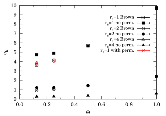
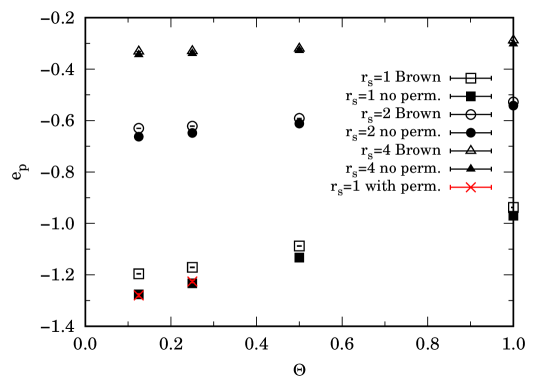
Figure 1: (color online) We show a comparison of our results at the three different values of density ($r_{s}=1,2,4$), with (with perm.) and without (no perm.) permutations, for the kinetic energy per particle (top panel) and the potential energy per particle (bottom panel) with the results of Brown et al. Brown et al. (2013) (Brown) as they are reported in the Tables 1 (no perm.) and 2 (with perm.).

In Fig. 2 we show our results for the radial distribution function M. P. Allen and D. J. Tildesley (1987), $g(r)$, for selected states of Table 1 at fixed temperature and at fixed density, respectively.

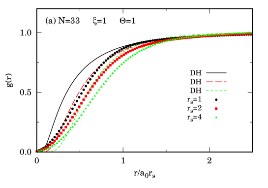
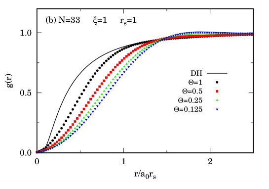
Figure 2: (color online) The radial distribution function for Jellium in selected states of Table 1, from algorithm A, at fixed temperature in the upper panel (a) and at fixed density in the lower panel (b). Also shown is the Debye-Hückel (DH) result Martin (1988) for the high temperature and low density limit, $g_{DH}(r)=\exp\left[-\frac{\Gamma}{r}\exp\left(-\sqrt{3\Gamma}r\right)\right]$.

As outlined in the previous section we repeated the calculation for the low temperature cases $\xi=1,r_{s}=1,\Theta=0.25$ and $\Theta=0.125$ with our modified algorithm B, with $\epsilon=1/2$, able to sample the whole fermions configuration space including the necessary permutations. The result in these cases were encouraging and are shown in Table 2. They were much closer to the corresponding result of Brown et al. Brown et al. (2013) than the results obtained with the previous algorithm A: The kinetic energy, in the highest density case, is within a 5% at low temperatures. We also checked that the two algorithms, A and B, coincide at high temperature. This validates our algorithms A and B.

Table 2: Same as Table 1 but using our algorithm B in the high density low temperature simulations.

$M$	$r_{s}$	$\Theta$	$\Gamma$	$e_{0}$	$P_{0}$	$e_{k}^{\rm Brown}$	$e_{p}^{\rm Brown}$	$e_{k}$	$e_{p}$	$e_{t}$	$P$
977	1	0.25	1.368	4.307310	0.685530	4.12(4)	$-$1.171(1)	4.1(2)	$-$1.226(5)	2.9(2)	1.76(4)
1000	1	0.125	2.737	3.727579	0.593263	3.64(1)	$-$1.1961(5)	3.8(2)	$-$1.280(6)	2.5(2)	1.73(2)

In Fig. 3 we show our results for the radial distribution function for the $\xi=1,r_{s}=1,\Theta=0.125$ state obtained with the algorithm with the G sector switched off (A) and with the algorithm with the G sector switched on (B).

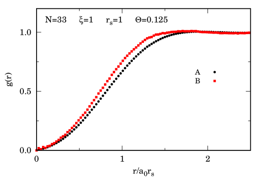
Figure 3: (color online) The radial distribution function for Jellium in the $\xi=1,r_{s}=1,\Theta=0.125$ state as obtained from our two algorithms A and B: The one without G sector and the one with G sector, respectively.

From the figure we see how the Fermi hole diminishes by the introduction of the permutations in the calculation.

VII Conclusions

We have successfully implemented the ideal fermion density matrix restriction on the path integral worm algorithm which is able to generate the necessary RPIMC moves during the simulation evolution thereby circumventing the otherwise inevitable sign problem. This allowed us to reach the finite, non-zero, temperature properties of a given fluid model of Fermi particles interacting through a given pair-potential. We worked in the canonical ensemble and applied our method to the Jellium fluid of Wigner. We explicitly compared our results with the previous canonical calculation of Brown et al. Brown et al. (2013) in the high density and low temperature regime where their algorithm had problems in sampling the path Ceperley (1992). Our results complement the ones of Brown et al. with the treatment of the high density $r_{s}\leq 4$ and low temperature cases which were found to be inaccurate by Bonitz et al. Schoof et al. (2015); Groth et al. (2016, 2017) who suggested an alternative algorithm to circumvent the systematic errors in Brown calculations Ceperley (1992).

The relevance of our study relies in the fact that our simulation method is different from both the method of Ceperley et al. Brown et al. (2013, 2014) who uses the fixed-nodes approximation in the canonical ensemble of a regular, and not worm, PIMC D. M. Ceperley (1995), and from the one of Bonitz et al. Schoof et al. (2011); Dornheim et al. (2015, 2016a); Groth et al. (2017) who combine configuration- and permutation-blocking PIMC. Our method is also different from other quantum Monte Carlo methods like the one of Malone et al. Malone et al. (2016) that agrees well with the one of Bonitz et al. at high densities and the direct PIMC one of Filinov et al. Filinov et al. (2015) that agrees well with Brown et al. at low density and moderate temperature. So our new algorithms add to the ones already used in the quest for an optimal way to calculate the properties of the fascinating Wigner’s Jellium model at finite, non zero, temperatures. We devised two different algorithms, A and B. In algorithm A we used a restricted, fixed-nodes, worm algorithm which never passes through the G sector. In algorithm B we used a restricted, fixed-nodes, worm algorithm with a G sector which has Masha and Ira always at the same imaginary time and at a given small spatial distance. In both cases the restriction of the fixed-nodes path integral is the one from a trial density matrix equal to the one of ideal fermions.

We obtained results for both the static structure (the radial distribution function) and various thermodynamic quantities (energy and pressure) for the Jellium model with $N=33$ fully polarized ($\xi=1$) electrons at high density and low temperature. Our results compares favorably with the ones of Brown et al. Brown et al. (2013) with a discrepancy on the kinetic energy, in the highest density case, up to a 0.5% at high temperatures (with our algorithm A) and up to 5% at low temperatures (with our algorithm B). Our results can also be compared with the later ones of Refs. Schoof et al. (2015); Groth et al. (2016) with which the agreement increases even further. This validates our algorithms which are alternative to the ones that have already been used in the literature.

We expect in the near future to explicitly determine the dependence of the Jellium properties (structural and thermodynamic) on the polarization $\xi$. We would also like to carry out a more comprehensive comparison with the results in the literature and to predict other results yet to be determined through quantum Monte Carlo methods, like the static structure function. Regarding improvements to the algorithm we would like to implement the use of better approximations for the action in the path integral and a search for better trial density matrices to guide the fixed-nodes at low temperatures or the implementation of the released-nodes recipe.

Another important problem to solve is the one of calculating the superfluid fraction for fermions or superconducting fraction for electrons. The winding numbers that one is computing in RPIMC are not be sufficient to determine the superfluid fraction since there is the restriction on the paths.