Deep Semi-Martingale Optimal Transport

Abstract

We propose two deep neural network-based methods for solving semi-martingale optimal transport problems. The first method is based on a relaxation/penalization of the terminal constraint, and is solved using deep neural networks. The second method is based on the dual formulation of the problem, which we express as a saddle point problem, and is solved using adversarial networks. Both methods are mesh-free and therefore mitigate the curse of dimensionality. We test the performance and accuracy of our methods on several examples up to dimension 10. We also apply the first algorithm to a portfolio optimization problem where the goal is, given an initial wealth distribution, to find an investment strategy leading to a prescribed terminal wealth distribution.

1 Introduction

The optimal transport problem goes back to the work of Monge (1781) and aims at transporting a distribution $\mu$ to another distribution $\nu$ under minimum transport cost. It was later revisited by Kantorovich (1942), leading to the so-called Monge–Kantorovich formulation. In recent years, a fast-developing phase was spurred by a wide range of extensions and applications of the Monge–Kantorovich problem; interested readers can refer to the books by Rachev and Rüschendorf (1998), Villani (2003) and Villani (2008) for a comprehensive review. Although we have gained tremendous theoretical insight, the numerical solution of the problem remains challenging. When the dimension is less or equal to three, many state-of-art approaches are able to compute the global solution effectively; see, for example, Chow et al. (2019), Haber and Horesh (2015), Li et al. (2018), and the review by Zhang et al. (2020). Readers can refer to the books by Santambrogio (2015) and Peyré and Cuturi (2019), and the references therein for an overview of these approaches. However, many traditional methods rely on Euclidean coordinates and require spatial discretization. When the distributions live in spaces of dimension four or more, these traditional methods suffer from the curse of dimensionality. Under this situation, solving optimal transport problems using deep neural networks looks very attractive since it can avoid space discretization.

Artificial Neural Networks (ANNs) are at the core of the Deep Learning methodology. ANNs were first introduced long ago by McCulloch and Pitts (1943), but due to the tremendous increase in computing power they have been widely used in the recent years. When an ANN has two or more hidden layers, it is called a Deep Neural Network (DNN). Usually the calibration of an ANN is done by minimizing a loss function. When the loss function is an expectation, Stochastic Gradient Descent (SGD) is a natural adaptation of Gradient Descent to stochastic optimization problems. The DNN-SGD paradigm is well suited for solving scientific computing problems such as stochastic control problems (e.g., Han and E 2016, Huré et al. 2021, Bachouch et al. 2021) or partial differential equations (PDEs) in very high dimension (e.g., Weinan et al. 2017, Sirignano and Spiliopoulos 2018 and Huré et al. 2019), thanks to its ability to overcome the curse of dimensionality. A comprehensive review of the numerical and theoretical advances in solving PDE and BSDE with deep learning algorithms can be found in Han and Jentzen (2020).

Recent years witnessed the emergence of research on solving optimal transport problems with neural networks. Ruthotto et al. (2020) used a residual network (ResNet) to approximately solve high-dimensional mean-field games by combining Lagrangian and Eulerian viewpoints. In the numerical experiment, they solved a dynamical optimal transport problem as a potential mean-field game. Henry-Labordère (2019) introduced Lagrange multipliers associated with the two marginal constraints and proposed a Lagrangian algorithm to solve martingale optimal transport using neural networks. However, for the sake of simplicity, this work only focuses on cost functions satisfying a martingale condition. Eckstein and Kupper (2019) studied optimal transport problem with an inequality constraint; their algorithm penalizes the optimization problem in its dual representation.

In this paper, we study optimal transport by semi-martingales as introduced in Tan and Touzi (2013) and we use deep learning to estimate the optimal drift and diffusion coefficients.

In particular, we propose two neural network-based algorithms in the paper.

• In the first one, we relax the terminal constraint by adding a penalty term to the loss function and solve it with a deep neural network.

• In the second one, we introduce the dual formulation of the problem and express it as a saddle point problem. In this case, we utilize adversarial networks to solve it.

These methods can be widely applied to solving optimal transport as well as stochastic optimal control problems. The two methods do not need spatial discretization and hence can be potentially used for high-dimensional problems. We illustrate our method with an application in finance, where we implement the first algorithm to the problem of optimal portfolio selection with a prescribed terminal density studied in Guo et al. (2020).

Our paper is organized as follows. In Section 2, we formulate the optimal transport problem and introduce the primal problem, adding a penalization to the expected cost function. To solve this problem, we propose a deep neural network-based algorithm and present the corresponding numerical results in Section 3. In Section 4, we provide the dual representation of the primal problem and express it as a saddle point problem. Then we devise an algorithm using adversarial networks. We illustrate the numerical results in subsections 4.1 and 4.2, including a $10$-dimensional example. Finally, in Section 5, we implement the deep learning algorithm introduced in Section 3 for a financial application, namely solving the problem of steering a portfolio wealth towards a prescribed terminal density.

2 Problem formulation

Let $\mathcal{D}$ be a Polish space equipped with its Borel $\sigma$-algebra. We denote as $C(\mathcal{D};\mathbb{R}^{d})$ the space of continuous functions on $\mathcal{D}$ with values in $\mathbb{R}^{d}$, $C_{b}(\mathcal{D};\mathbb{R}^{d})$ the space of bounded continuous functions and $C_{0}(\mathcal{D};\mathbb{R}^{d})$ the space of continuous functions, vanishing at infinity. Let $\mathcal{P}(\mathcal{D})$ be the space of Borel probability measures on $\mathcal{D}$ with a finite second moment, and $L^{1}(d\mu)$ be the space of $\mu$-integrable functions. Let $\mathbb{R}^{+}$ denote non-negative real numbers, $\mathbb{S}^{d}$ denote the set of $d\times d$ symmetric matrices and $\mathbb{S}_{+}^{d}\subset\mathbb{S}^{d}$ denote the set of positive semidefinite matrices. For convenience, we often use the notation $\mathcal{E}\coloneqq[0,1]\times\mathbb{R}^{d}$. We say that a function $\phi:\mathcal{E}\rightarrow\mathbb{R}$ belongs to $C_{b}^{1,2}(\mathcal{E})$ if $\phi\in C_{b}(\mathcal{E})$ and $(\partial_{t}\phi,\partial_{x}\phi,\partial_{xx}\phi)\in C_{b}(\mathcal{E};\mathbb{R},\mathbb{R}^{d},\mathbb{S}^{d})$.

Without loss of generality, we set the time horizon $T$ to be $1$. Let $\Omega\coloneqq(\omega\in C([0,1];\mathbb{R}^{d})),$ we denote by $\mathbb{F}=(\mathcal{F}_{t})_{t\in[0,1]}$ the filtration generated by the canonical process. The process $W$ is a $d$-dimensional standard Brownian motion on the filtered probability space $\left(\Omega,\mathcal{F},\mathbb{F},\mathbb{P}\right)$.

The stochastic process $(X_{t})_{t\in[0,1]}$ valued in $\mathbb{R}^{d}$ solves the SDE

$$dX_{t} =B(t,X_{t})dt+A(t,X_{t})dW_{t},$$ (1)

$$X_{0} =x_{0},$$ (2)

where $B:\mathcal{E}\rightarrow\mathbb{R}^{d}$ and $A:\mathcal{E}\rightarrow\mathbb{R}^{d\times d}$ is defined such that $AA^{\intercal}=\mathcal{A}$.

We denote by $\rho_{t}\coloneqq\mathbb{P}\circ X_{t}^{-1}\in\mathcal{P}(\mathbb{R}^{d})$ the distribution of $X_{t}$. In this problem, we are given the initial distribution of the state variable $\rho_{0}\in\mathcal{P}(\mathbb{R}^{d})$, and a prescribed terminal distribution $\bar{\rho}_{1}\in\mathcal{P}(\mathbb{R}^{d})$. We define a convex cost function $F:\mathbb{R}^{d}\times\mathbb{S}^{d}\rightarrow\mathbb{R}^{+}\cup\{+\infty\}$ where $F(B,\mathcal{A})=+\infty$ if $\mathcal{A}\notin\mathbb{S}_{+}^{d}$.

Given $\rho_{0}$ and suitable processes $(A_{t})_{t\in[0,1]},(B_{t})_{t\in[0,1]}$, the distribution of $X_{1}$ is $\rho_{1}\coloneqq\mathbb{P}\circ X_{1}^{-1}$. We introduce the penalty function $C(\rho_{1},\bar{\rho}_{1})$, whose role will be to penalize the deviation of $\rho_{1}$ from the target $\bar{\rho}_{1}$.

Now we are interested in the following minimization problem:

Problem 1.

With a given initial distribution $\rho_{0}$ and a prescribed terminal distribution $\bar{\rho}_{1}$, we want to solve the infimum of the functional

$$V(\rho_{0},\bar{\rho}_{1})=\inf_{\rho,B,\mathcal{A}}\left\{\int_{\mathcal{E}}F(B_{t},\mathcal{A}_{t})d\rho(t,x)+C(\rho_{1},\bar{\rho}_{1})\right\},$$ (3)

over all $(\rho,B,\mathcal{A})\in\mathcal{P}(\mathbb{R}^{d})\times\mathbb{R}^{d}\times\mathbb{S}^{d}$ satisfying the initial distribution

$$\rho(0,x) =\rho_{0}(x) \quad\forall x\in\mathbb{R}^{d},$$ (4)

and the Fokker–Planck equation

$$\partial_{t}\rho(t,x)+\nabla_{x}\cdot(B(t,x)\rho(t,x))-\frac{1}{2}\sum_{i,j}\partial_{ij}(\mathcal{A}_{i,j}(t,x)\rho(t,x)) =0 \quad\forall(t,x)\in\mathcal{E}.$$ (5)

Because the objective function (3) is a trade-off between the cost function $F$ and the penalty $C$, the optimal $\rho,\mathcal{A},B$, if it exists, will not in general ensure that $\rho_{1}=\bar{\rho}_{1}$, unless the penalty function is

$$C(\rho_{1},\bar{\rho}_{1})=\begin{cases}0&\text{ if }\rho_{1}=\bar{\rho}_{1},\\ +\infty&\;\text{if}\>\rho_{1}\neq\bar{\rho}_{1},\end{cases}$$ (6)

and one recovers the “usual” semi-martingale optimal transport problem.

We make the following assumptions which will hold throughout the paper.

Assumption 1.

For $t\in(0,1]$ the probability measure $\rho_{t}$ is absolutely continuous with respect to the Lebesgue measure.

Assumption 2.

The penalty function $C(\cdot,\bar{\rho}_{1}):\mathcal{P}(\mathbb{R}^{d})\rightarrow\mathbb{R}^{+}$ is convex, lower semi-continuous with respect to the weak-$\ast$ convergence of $\rho_{1}$, and $C(\rho_{1},\bar{\rho}_{1})=0$ if and only if $\rho_{1}=\bar{\rho}_{1}$.

Assumption 3.

 

1. For $(t,x)\in\mathcal{E}$ the function $(B,\mathcal{A})\to F(B,\mathcal{A})$ is non-negative, lower semi-continuous and strictly convex.

2. There exist constants $m>1$ and $k>0$ such that for all $(t,x)\in\mathcal{E}$ there holds

   $$\left|B\right|^{m}+\left|\mathcal{A}\right|^{m}\leq k\left(1+F(B,\mathcal{A})\right).$$

3. For all $(t,x)\in\mathcal{E}$, we have

   $$\mathbb{E}\Bigl{[}\int_{0}^{1}\left|B\right|+\left|\mathcal{A}\right|dt\Bigr{]}<\infty,$$

   where $\left|\cdot\right|$ is the $L^{1}$-norm.

With Assumptions 2 and 3, we can get the following existence and uniqueness result for the minimizer of Problem 1 using similar convex minimization techniques as in Loeper (2006, Proposition 2). We refer the interested readers to Loeper (2006) for the detailed proof.

Theorem 1.

Let us define

$$I(\rho,B,\mathcal{A})=\int_{\mathcal{E}}F(B_{t},\mathcal{A}_{t})d\rho(t,x)+C(\rho_{1},\bar{\rho}_{1}).$$

Under Assumptions 2 and 3, if $I(\rho,B,\mathcal{A})$ is finite, then there exists a unique minimizer $(\rho,B,\mathcal{A})\in\mathcal{P}(\mathbb{R}^{d})\times\mathbb{R}^{d}\times\mathbb{S}^{d}$ for Problem 1 satisfying constraints (4) and (5).

3 Deep Neural Network based Algorithm

In this section, we devise an algorithm to solve problem 1 by using deep learning. Note that given processes $(B_{t})_{t\in[0,1]}$, $(A_{t})_{t\in[0,1]}$ and $\rho_{0}$, the density process $(\rho_{t})_{t\in(0,1]}$ is fully determined (up to suitable regulation assumptions on $B$ and $A$). Hence, our goal is to use neural networks to search for the optimal $(B_{t})_{t\in[0,1]}$ and $(A_{t})_{t\in[0,1]}$, which minimize the objective function.

We discretize the period $[0,1]$ into $N$ constant time steps and construct a neural network $\theta_{n}$ for each time step $n\in[0,N-1]$. We use multilayer feedforward neural networks in our application. At each time step, we wish to approximate the drift and diffusion coefficient with the neural network, i.e., $(B_{n},A_{n})\approx\theta_{n}(X_{n})$, where $B_{n}\in\mathbb{R}^{d},A_{n}\in\mathbb{R}^{d\times d}$. Feedforward neural networks approximate complicated nonlinear functions by a composition of simpler functions, namely

$$(B_{n},A_{n})\approx\theta_{n}(X_{n})=g_{n}^{J}\circ g_{n}^{J-1}\circ\cdots\circ g_{n}^{1}(X_{n}).$$

For each layer, $g_{n}^{j}$ is

$$g_{n}^{j}(X_{n})=\sigma^{j}\left(X_{n}\textbf{W}_{n}^{j}+\textbf{b}_{n}^{j}\right),$$ (7)

where $\textbf{W}_{n},\textbf{b}_{n}$ are the weight matrices and bias vectors, respectively. Here, $\sigma^{j}(\cdot)$ is a component-wise nonlinear activation function, like sigmoid, ReLU, tanh, etc. In our paper, we use Leaky ReLU for all the hidden layers. For the output layer, $\sigma^{j}(\cdot)$ is the identity function.

We denote by $M$ the number of Monte Carlo paths. For a particular path $m\in[1,M]$, with $B_{n}^{m},A_{n}^{m}$ and $X_{n}^{m}$, we can compute the state variable in the next time step from the dynamics

$$X_{n+1}^{m}=X_{n}^{m}+B_{n}^{m}\Delta t+A_{n}^{m}\Delta W_{n}^{m},\quad\forall m\in[1,M],n\in[0,N-1].$$

At the final time step $N$, we can get $M$ samples of terminal wealth $X_{N}$ from the Monte Carlo paths. With these samples, we can estimate the empirical terminal distribution $\rho_{1}$ using kernel density estimation (KDE). In particular, we use the Gaussian kernel $K_{\mathbf{H}}(x)=(2\pi)^{-d/2}|\mathbf{H}|^{-\frac{1}{2}}e^{-\frac{1}{2}x^{\intercal}\mathbf{H}^{-1}x}$ with an appropriate bandwidth matrix $\mathbf{H}\in\mathbb{S}^{d}$. Then the terminal density is estimated as $\tilde{\rho}_{1}(x)\coloneqq\frac{1}{M}\sum_{m=1}^{M}K_{\mathbf{H}}(x-X_{N}^{m})$. Because the kernel density estimation is not an unbiased estimator of the true density, an error is generated from estimating $\rho_{1}$ with $\tilde{\rho}_{1}$. To address this issue, we also estimate $\bar{\rho}_{1}$ with the same KDE and use the estimated $\tilde{\bar{\rho}}_{1}$ as the target density in the training. To be precise, we first generate a sample $\tilde{\mathbf{x}}=(\tilde{x}_{1},\tilde{x}_{2},...,\tilde{x}_{M^{\prime}})$ of size $M^{\prime}$ from the target density $\bar{\rho}_{1}(x)$. Then we estimate $\bar{\rho}_{1}(x)$ with $\tilde{\bar{\rho}}_{1}(x)\coloneqq\frac{1}{M^{\prime}}\sum_{i=1}^{M^{\prime}}K_{\mathbf{H}}(x-\tilde{x}_{i})$.

Finally, the objective function in (3) can be naturally used as the loss function in the training,

$$L(\theta_{n,n\in[0,N-1]})=\mathbb{E}\Bigl{[}\sum_{n=0}^{N-1}F(\theta_{n}(X_{n}))\Delta t\Bigr{]}+C(\tilde{\rho}_{1},\tilde{\bar{\rho}}_{1}).$$

Then the training will search for the optimal neurons $\hat{\theta}_{n,n\in[0,N-1]}$ where

$$\hat{\theta}_{n,n\in[0,N-1]}=\arg\inf_{\theta}\left\{\frac{1}{M}\sum_{m=1}^{M}\biggl{\{}\sum_{n=0}^{N-1}F(\theta_{n}(X_{n}^{m}))\Delta t\biggr{\}}+C(\tilde{\rho}_{1},\tilde{\bar{\rho}}_{1})\right\}.$$

We depict the above process in a flowchart (Figure 1), and the complete Deep Neural Network algorithm for Problem 1 is stated in Algorithm 1.

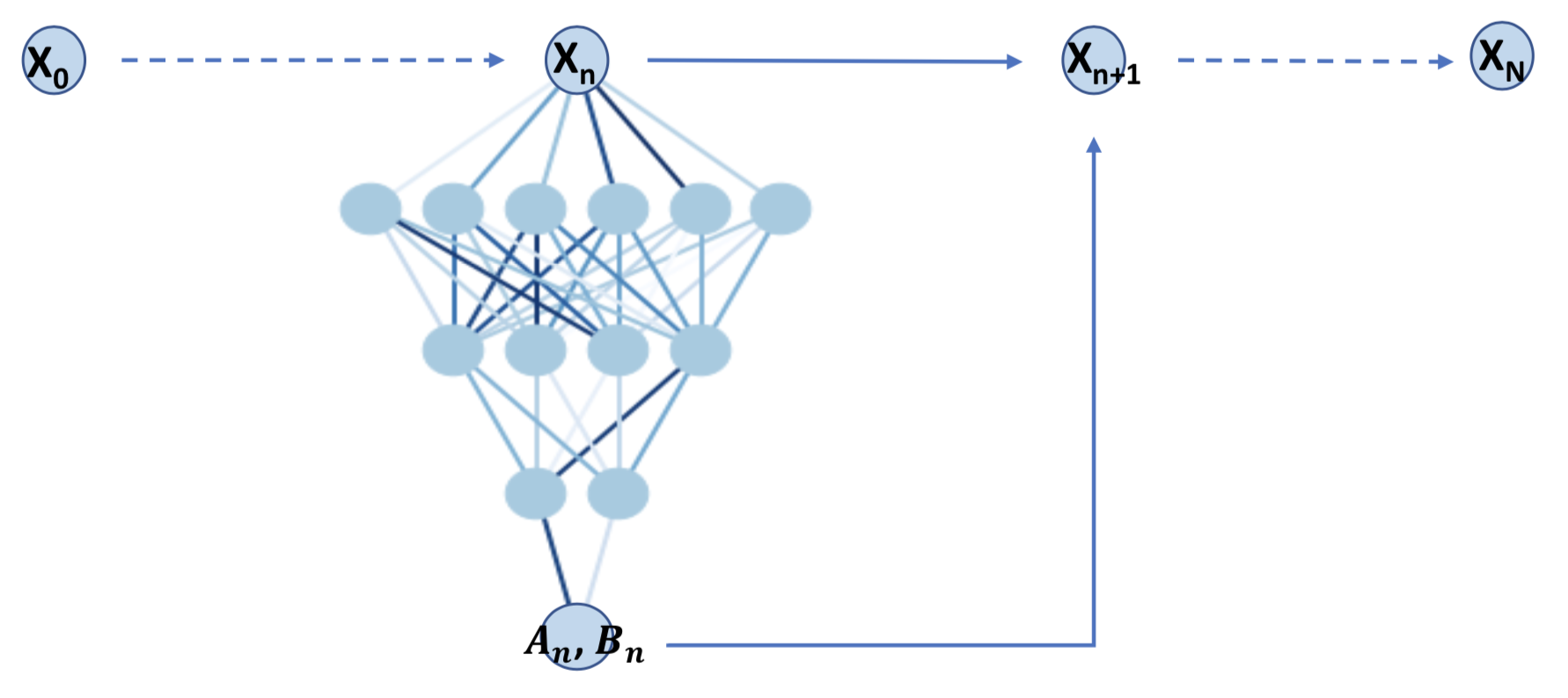
Figure 1: Structure of the DNN for one path

Starting from the initial condition $X_{0}^{m}=x_{0}\,\forall m\in[1,M]$.

for epoch $=1:100$ do

       for $n=0:N-1$ do

             With neurons $\theta_{n}$, input $X_{n}^{m}$, output $B_{n}^{m},A_{n}^{m}=\theta_{n}(X_{n}^{m})$; $X_{n+1}^{m}=X_{n}^{m}+B_{n}^{m}\Delta t+A_{n}^{m}\Delta W_{n}^{m}$;

       end for

      Estimate the terminal distribution of $X_{N}$ with KDE as $\tilde{\rho}_{1}$; Estimate $\tilde{\bar{\rho}}_{1}$ from $\bar{\rho}_{1}$ with the same KDE; Define Loss function $L=\frac{1}{M}\sum_{m=1}^{M}\biggl{\{}\sum_{n=0}^{N-1}F(B_{n}^{m},A_{n}^{m}(A_{n}^{m})^{\intercal})\Delta t\biggr{\}}+C(\tilde{\rho}_{1},\tilde{\bar{\rho}}_{1})$; Train the neurons and update $\theta_{n,n\in[0,N-1]}$;

end for

Get the optimal $\hat{\theta}_{n,n\in[0,N-1]}$.

Algorithm 1 Deep Neural Network for Problem 1

3.1 Numerical Results

In this section, we validate Algorithm 1 with an example where

$$F(B,\mathcal{A}) =\left\|B\right\|^{2},$$ (8)

$$C(\rho_{1},\bar{\rho}_{1}) =\frac{\lambda}{2}\int_{\mathbb{R}}(\rho_{1}-\bar{\rho}_{1})^{2}dx.$$ (9)

The parameter $\lambda$ in (9) is the intensity of the penalization. To push $\rho_{1}$ as close as possible to the target $\bar{\rho}_{1}$, we want $\lambda$ be to large and we will let $\lambda=5000$ in this case. We start from an initial state $x_{0}=\begin{bmatrix}5.0\\ 5.0\end{bmatrix}$, and the target distribution set to be a bivariate normal $\bar{\rho}_{1}=\mathcal{N}\left(\begin{bmatrix}5.5\\ 6.0\end{bmatrix},\begin{bmatrix}0.25&0.10\\ 0.10&0.25\end{bmatrix}\right)$.

In the training, we construct a $5$-layer network with neurons $[100,80,60,60,40]$. The output of the network is of size $2\times 3$, out of which the $2\times 1$ column represents the drift $B_{n}$ and the $2\times 2$ matrix represents the diffusion coefficient $A_{n}$. We use a batch size of $2000$ and the Adam optimizer with a learning rate $1\times 10^{-4}$. We trained the network for $100$ epochs in total.

From the training, we get an empirical terminal density $\rho_{1}$ with mean $\begin{bmatrix}5.509\\ 5.994\end{bmatrix}$ and covariance matrix $\begin{bmatrix}0.253&0.098\\ 0.098&0.246\end{bmatrix}$. We can see that the mean and covariance of the empirical terminal density are very close to the target ones.

The contours of the empirical distribution and the target distribution are presented in Figure 2. In the later section, we will introduce a metric to measure the performance of the trained dataset.

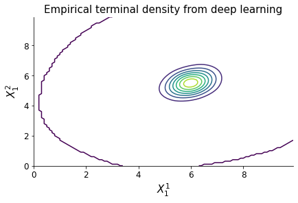
(a) Density of $X_{1}$ from Algorithm 1

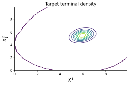
(b) Target Density of $X_{1}$

Figure 2: Contours with a bivariate normal target distribution

3.2 Merged Network

The architecture described in Algorithm 1 consists of training $N$ different feedforward neural networks (one per time step). This architecture generates a possibly high number of weights and bias to be estimated. Another possibility is to use one single feedforward neural network for all time steps. At each time step, besides the state variable $X_{n}$, we also feed the time $n$ into the network. We refer to this alternative architecture as a feedforward merged network. The training process for this merged network is illustrated in Figure 3, and the algorithm is summarized in Algorithm 2. The advantage of this architecture is that, instead of training a list of networks $\theta_{n,n\in[0,N-1]}$, we only need to train one network $\theta$ in this algorithm, which significantly reduces the number of neurons and the complexity of the training.

The numerical experiment gives us a similar result to the one from Algorithm 1; hence we are not presenting them repeatedly. As we observed from the experiment, each epoch’s speed of training is faster, but it will need relatively more epochs to converge to the final value.

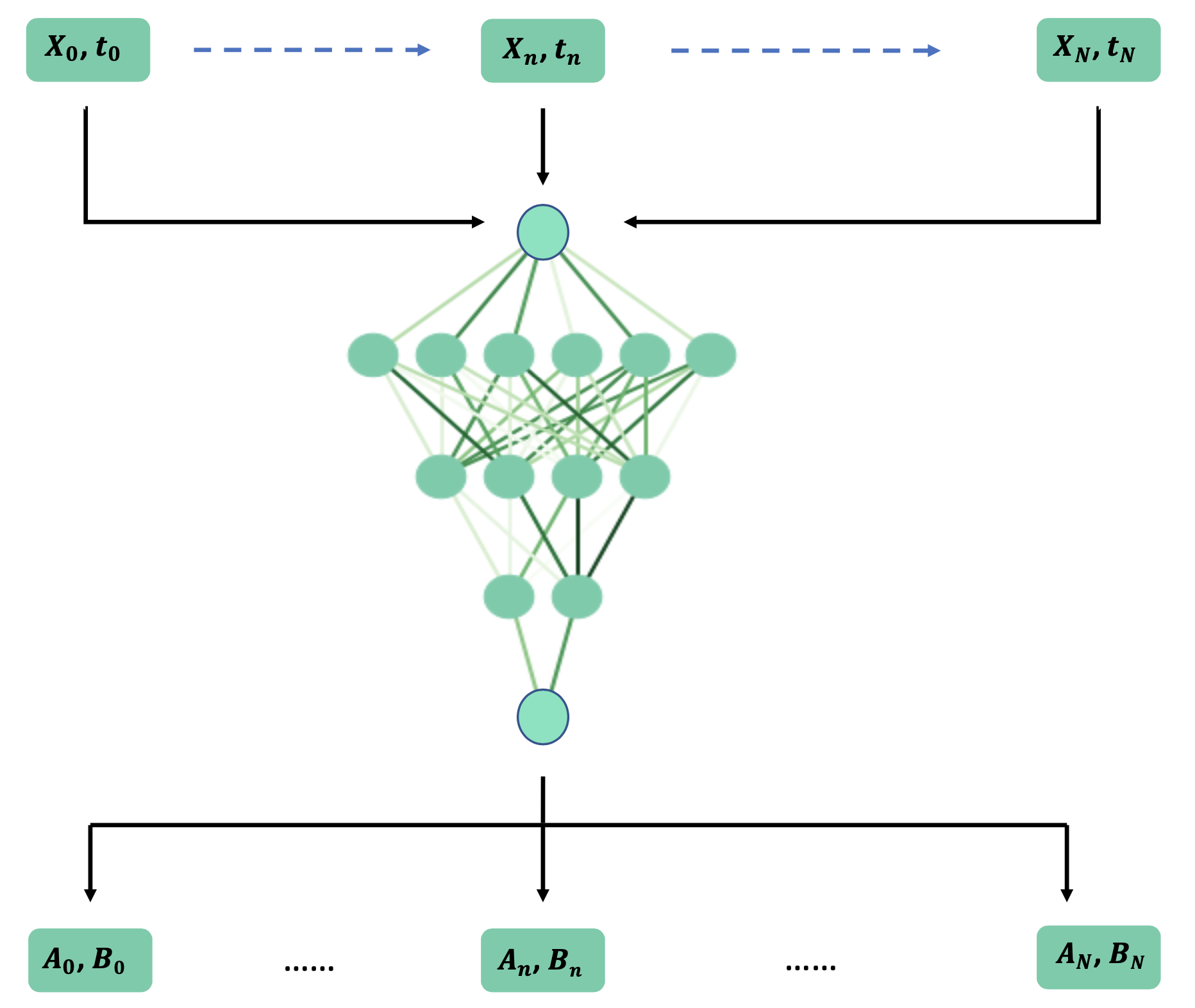
Figure 3: Structure of the merged network

Starting from the initial condition $X_{0}^{m}=x_{0}\,\forall m\in[1,M]$.

for epoch $=1:100$ do

       for $n=0:N-1$ do

             With neurons $\theta$, input $X_{n}^{m}$ and $n$, output $B_{n}^{m},A_{n}^{m}=\theta(X_{n}^{m},n)$; $X_{n+1}^{m}=X_{n}^{m}+B_{n}^{m}\Delta t+A_{n}^{m}\Delta W_{n}^{m}$;

       end for

      Estimate the terminal distribution of $X_{N}$ with KDE as $\tilde{\rho}_{1}$; Estimate $\tilde{\bar{\rho}}_{1}$ from $\bar{\rho}_{1}$ with the same KDE; Loss function $L=\frac{1}{M}\sum_{m=1}^{M}\biggl{\{}\sum_{n=0}^{N-1}F(B_{n}^{m},A_{n}^{m}(A_{n}^{m})^{\intercal})\Delta t\biggr{\}}+C(\tilde{\rho}_{1},\tilde{\bar{\rho}}_{1})$; Train the neurons with the Adam optimizer and update $\theta$;

end for

Get the optimal $\hat{\theta}$.

Algorithm 2 Deep Neural Network for Problem 1 with a merged network

4 Adversarial Network Algorithm for the dual problem

In this section, we first introduce the dual formulation of Problem 1 and express it as a saddle point problem. Then we propose an Adversarial Network-based algorithm to solve it, where we demonstrate high dimensional numerical examples. This algorithm is inspired by Generative Adversarial Networks (GANs), which were first introduced in Goodfellow et al. (2014). GANs have enjoyed great empirical success in image generating and processing. The principle behind GANs is to interpret the process of generative modeling as a competing game between two (deep) neural networks: a generator and a discriminator. The generator network attempts to generate data that looks similar to the training data, and the discriminator network tries to identify whether the input sample is faked or true. GANs recently have attracted interests in the finance field, including simulating financial time-series data (e.g., Wiese et al. 2020, Zhang et al. 2019) and for asset pricing models (Chen et al. 2019).

To recover the optimal transport problem, we can use an indicator function (6) as the penalty functional. Now we present the duality result for Problem 1. The following theorem is stated in Tan and Touzi (2013).

Theorem 2.

When $C(\rho_{1},\bar{\rho}_{1})$ is defined as (6), there holds

$$V(\rho_{0},\bar{\rho}_{1}) =\sup_{\phi_{1}}\left\{\int_{\mathbb{R}^{d}}\phi_{1}d\bar{\rho}_{1}-\phi_{0}d\rho_{0}\right\},$$ (10)

where the supremum is running over all $\phi_{1}\in C_{b}^{2}(\mathbb{R}^{d})$ and $\phi_{0}$ is a viscosity solution of the Hamilton–Jacobi–Bellman equation

$$\begin{cases}-\partial_{t}\phi-\sup_{B\in\mathbb{R}^{d},\mathcal{A}\in\mathbb{S}^{d}}\Bigl{[}B\cdot\nabla_{x}\phi+\frac{1}{2}tr(\mathcal{A}\nabla_{x}^{2}\phi)-F(B,\mathcal{A})\Bigr{]}=0,&\text{in }[0,1)\times\mathbb{R}^{d},\\ \phi(1,x)=\phi_{1}(x),&\text{on }[1]\times\mathbb{R}^{d}.\end{cases}$$ (11)

The function $\phi(0,x)$ can be expressed as

$$\phi(0,x)=\sup_{B\in\mathbb{R}^{d},\mathcal{A}\in\mathbb{S}^{d}}\mathbb{E}\left[\phi_{1}(X_{1})-\int_{0}^{1}F(B,\mathcal{A})dt|X_{0}=x_{0}\right].$$ (12)

Starting from an initial state $x_{0}\in\mathbb{R}^{d}$, the initial density $\rho_{0}(x)=\delta(x-x_{0})$, hence $\int_{\mathbb{R}^{d}}\phi_{0}d\rho_{0}=\phi_{0}(x_{0})$. Then we can substitute the expression (12) into the dual form (10), and the dual formulation can be written as a saddle point problem:

$$V(\rho_{0},\bar{\rho}_{1})=\sup_{\phi_{1}}\inf_{B\in\mathbb{R}^{d},\mathcal{A}\in\mathbb{S}^{d}}\left\{\int_{\mathbb{R}^{d}}\phi_{1}d\bar{\rho}_{1}-\mathbb{E}\left[\phi_{1}(X_{1})-\int_{0}^{1}F(B,\mathcal{A})dt|X_{0}=x_{0}\right]\right\}.$$ (13)

This dual saddle point formulation of the optimal transport problem is reminiscent of GANs: GANs can be interpreted as minimax games between the generator and the discriminator, whereas our problem is a minimax game between $\phi_{1}$ and $(\mathcal{A},B)$.

Inspired by this connection, we can use Adversarial Networks to estimate the value (13). GANs is also applied by Guo et al. (2019) to solve a robust portfolio allocation problem. Our Adversarial Network consists of two neural networks; one generates $\phi_{1}$ (referred to as $\phi_{1}$-generator, denoted by $\Phi$), the other generates $A$ and $B$ (referred to as $AB$-generator, denoted by $\theta$). The two networks are trained iteratively: In the first phase, we train the $AB$-generator with a loss function $L_{1}=-\mathbb{E}\left[\phi_{1}(X_{1})-\int_{0}^{1}F(B,\mathcal{A})dt|X_{0}=x_{0}\right]$. In the second phase, given the output $X_{1}$ from the $AB$-generator, we train the $\phi_{1}$-generator with a loss function $L_{2}=-\int_{\mathbb{R}^{d}}\phi_{1}d\bar{\rho}_{1}+\mathbb{E}\left[\phi_{1}(X_{1})-\int_{0}^{1}F(B,\mathcal{A})dt|X_{0}=x_{0}\right]$.

When the dimension $d\geq 3$, the bottleneck in this algorithm is to compute $\int_{\mathbb{R}^{d}}\phi_{1}d\bar{\rho}_{1}$ efficiently. To address this issue, we can use Monte Carlo integration. In particular, we sample $\mathcal{I}$ points $\bar{x}_{i}\in\mathbb{R}^{d}$ $(i\in[1,\mathcal{I}])$ from the target distribution $\bar{\rho}_{1}$. Then we can estimate $\int_{\mathbb{R}^{d}}\phi_{1}d\bar{\rho}_{1}$ with $\frac{1}{\mathcal{I}}\sum_{i=1}^{\mathcal{I}}\phi_{1}(\bar{x}_{i})$. In this case, this Adversarial Network-based scheme is mesh-free. It can now avoid the curse of dimensionality and has the potential to be applied to high dimensional problems.

We use a merged network for the $AB$-generator in this algorithm. A demonstration of the training process is illustrated in Figure 4. The detailed algorithm is summarized in Algorithm 3.

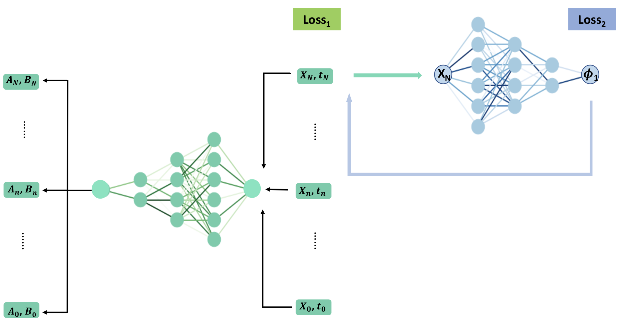
Figure 4: Adversarial Network algorithm with a merged network for the dual problem

Sample $\mathcal{I}$ points $\bar{x}_{i}\in\mathbb{R}^{d}$ $(i\in[1,\mathcal{I}])$ from the target distribution $\bar{\rho}_{1}$.

Starting from the initial condition $X_{0}^{m}=x_{0}\,\forall m\in[1,M]$:

for epoch $=1:\text{number of epochs}$ do

       Phase 1: train the $AB$-generator for time step $n=1:N-1$ do

             With the network $\theta$, input $\{X_{n}^{m}\}_{m=1}^{M}$ and time step $n$, outputs $(B_{n}^{m},A_{n}^{m})=\theta(X_{n}^{m},n)$; $X_{n+1}^{m}=X_{n}^{m}+B_{n}^{m}\Delta t+A_{n}^{m}\Delta W_{n}$;

       end for

      Loss function $L_{1}=-\frac{1}{M}\sum_{m=1}^{M}\left[\Phi(X_{N}^{m})-\sum_{n=0}^{N-1}F(B_{n}^{m},A_{n}^{m}(A_{n}^{m})^{\intercal})\Delta t\right]$; Train the neurons with the Adam optimizer and update $\theta$. Phase 2: train the $\phi_{1}$-generator With the network $\Phi$, input $\{X_{N}^{m}\}_{m=1}^{M}$, output $\phi_{1}(X_{N}^{m})=\Phi(X_{N}^{m})$; With the same network $\Phi$, inputs $\bar{x}_{i},\forall i\in[1,\mathcal{I}]$, outputs $\Phi(\bar{x}_{i})$; Loss function $L_{2}=-\frac{1}{\mathcal{I}}\sum_{i=1}^{\mathcal{I}}\Phi(\bar{x}_{i})+\frac{1}{M}\sum_{m=1}^{M}\left[\Phi(X_{N}^{m})-\sum_{n=0}^{N-1}F(B_{n}^{m},A_{n}^{m}(A_{n}^{m})^{\intercal})\Delta t\right]$; Train the neurons with the Adam optimizer and update $\Phi$.

end for

Algorithm 3 Adversarial Network algorithm with a merged network for the dual problem

4.1 Numerical Results

First, we start with a one-dimensional toy example to assess the quality of Algorithm 3. We choose a target distribution $\bar{\rho}_{1}=\mathcal{N}(6,1)$, a cost function $F(B,\mathcal{A})=(\mathcal{A}-0.1)^{2}$ and solve for $V(\rho_{0},\bar{\rho}_{1})=\sup_{\phi_{1}}\left\{\int_{\mathbb{R}}\phi_{1}d\bar{\rho}_{1}-\phi_{0}d\rho_{0}\right\}$.

In Figure 5a, we plot the target distribution and the distribution of $X_{1}$ learnt by the Adversarial Networks; in Figure 5b, we show the corresponding loss function during the training. We can see that our algorithm works well in terms of attaining the target density.

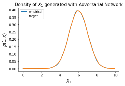
(a) Distribution of $X_{1}$ learnt by the Adversarial Network

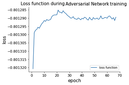
(b) Loss function

Figure 5: Dimension $d=1$, $\bar{\rho}_{1}=\mathcal{N}(6,1)$

Next, we demonstrate a two-dimensional example. We let $X_{n}\in\mathbb{R}^{2}$, and we generate the drift $B_{n}\in\mathbb{R}^{2}$ and the diffusion coefficient $A_{n}\in\mathbb{R}^{2\times 2}$ with the deep neural network. We again start from an initial state $x_{0}=\begin{bmatrix}5.0\\ 5.0\end{bmatrix}$, and let the cost function $F(B,\mathcal{A})=\left\|B\right\|^{2}$ and the target distribution set to be a bivariate normal $\bar{\rho}_{1}=\mathcal{N}\left(\begin{bmatrix}5.5\\ 6.0\end{bmatrix},\begin{bmatrix}0.25&0.10\\ 0.10&0.25\end{bmatrix}\right)$.

We construct two networks for $(A,B)$ and $\phi_{1}$, respectively. The $AB$-generator has $4$ layers with neurons $[40,30,20,10]$ and the $\phi_{1}$-generator has $4$ layers with neurons $[80,60,40,40]$. We use a mini-batch SGD algorithm with a batch size of $1000$ and Adam optimizer with learning rate $1\times 10^{-4}$.

The empirical terminal density $\rho_{1}$ after the training has mean $\begin{bmatrix}5.497\\ 6.007\end{bmatrix}$ and covariance matrix $\begin{bmatrix}0.253&0.099\\ 0.099&0.251\end{bmatrix}$, which are very close to the target mean and covariance. The contours of the empirical and target distributions are shown in Figure 6. This result is similar to the one we got from Algorithm 1.

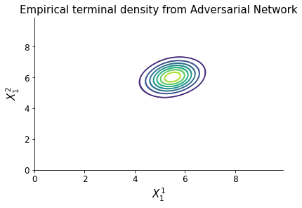
(a) Contour of $\rho_{1}$ from the Adversarial Network

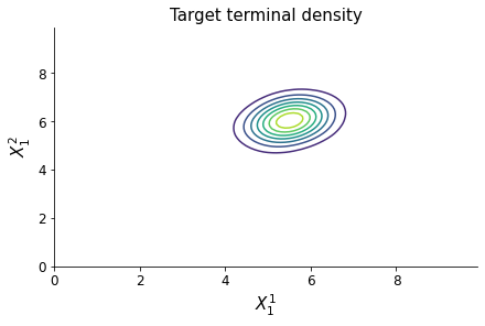
(b) Contour of $\bar{\rho}_{1}$

Figure 6: Dimension $d=2$, bivariate normal target distribution

4.2 Higher dimensional examples

In this section, we apply the Adversarial Network-based algorithm to high dimensional examples. When the dimension $d\geq 3$, Algorithm 1 will be less effective. It is because the kernel density estimation requires a spatial discretization, and the number of grid will increase exponentially with the dimension. The estimation becomes less accurate, and the computing cost will be expensive in this way. However, the Adversarial Network-based algorithm for the dual problem is free from spatial discretization. Hence it is less affected by an increase in dimension.

In the following, we use a cost function $F(B,\mathcal{A})=\left\|B\right\|^{2}+\left\|\mathcal{A}\right\|^{2}$ and solve the dual problem (13) with $d=5$ and $d=10$, respectively.

In the $5-$d example, we set $x_{0}=\begin{bmatrix}5.0\\ 5.0\\ 5.0\\ 5.0\\ 5.0\end{bmatrix}$, and let $\bar{\rho}_{1}$ be a multivariate normal distribution, where $\bar{\rho}_{1}=\mathcal{N}\left(\begin{bmatrix}5.5\\ 6.0\\ 5.8\\ 6.0\\ 6.2\end{bmatrix},\begin{bmatrix}0.25&0.10&0.10&0.10&0.10\\ 0.10&0.25&0.10&0.10&0.10\\ 0.10&0.10&0.25&0.10&0.10\\ 0.10&0.10&0.10&0.25&0.10\\ 0.10&0.10&0.10&0.10&0.25\end{bmatrix}\right)$ .

Because the dimension is higher and the cost function is more complicated in this case, we need a bigger and deeper network. The $AB$-generator now has $5$ layers with neurons $[400,300,200,200,150]$, the $\phi_{1}$-generator keeps the same as before. Using 20,000 out-of-sample points of $X_{1}$ from the trained model, the empirical terminal density $\rho_{1}$ from Algorithm 3 has mean $\begin{bmatrix}5.4929\\ 5.9749\\ 5.7855\\ 5.9825\\ 6.1944\end{bmatrix}$ and covariance matrix $\begin{bmatrix}0.2515&0.1041&0.1038&0.1037&0.1011\\ 0.1041&0.2372&0.0926&0.0937&0.0885\\ 0.1038&0.0926&0.2541&0.1103&0.0979\\ 0.1037&0.0937&0.1103&0.2686&0.0906\\ 0.1011&0.0885&0.0979&0.0906&0.2475\end{bmatrix}$.

We use graphical tools to help us assess if the data plausibly come from the prescribed multivariate normal distribution. First, we compare the marginal distributions of $\rho_{1}$ with the ones of $\bar{\rho}_{1}$ in Figure 7. We can see that the empirical marginal distributions are consistent with the theoretical ones for all of the $5$ marginals. Furthermore, we make a Q-Q plot for each margin, where we plot the quantiles of the empirical marginal distribution against the quantiles of the theoretical normal distribution. As we can see in Figure 8, for every margin, the points form a roughly straight line. There are a few outliers at the two ends of the Q-Q plots, which is to be expected as Monte Carlo methods converge slowly for extreme values. Overall, the above two figures, in addition to the mean and covariance matrix, can verify the assumption that our dataset follows the target distribution $\bar{\rho}_{1}$ closely.

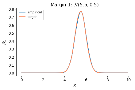
(a) margin 1

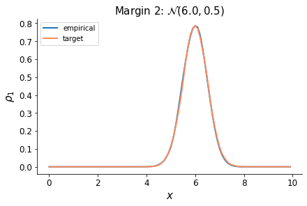
(b) margin 2

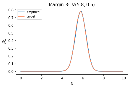
(c) margin 3

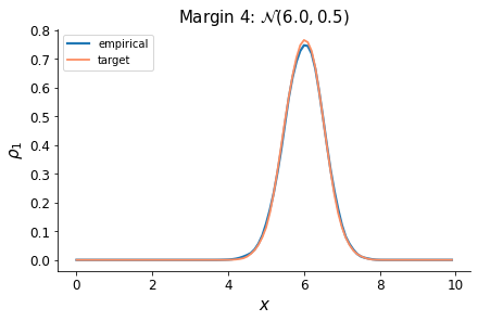
(d) margin 4

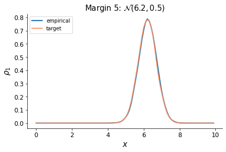
(e) margin 5

Figure 7: Marginal distributions of the 5-d sample

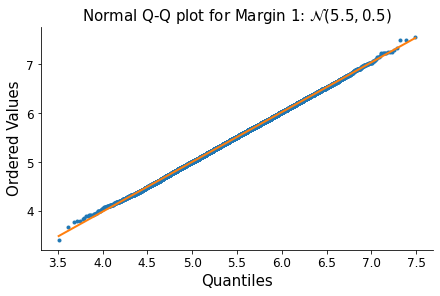
(a) margin 1

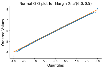
(b) margin 2

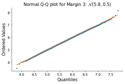
(c) margin 3

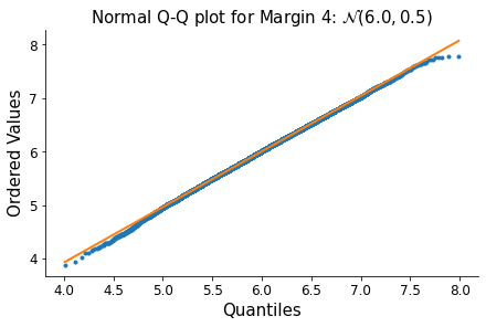
(d) margin 4

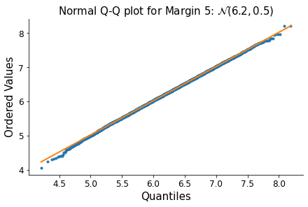
(e) margin 5

Figure 8: Normal Q-Q plot for margins

Next, we project the dataset $X_{1}$ on a random direction $b\in\mathbb{R}^{5}$. For a multivariate Gaussian distribution, the distribution after an affine transformation is univariate Gaussian. Let $X_{\text{affine}}=X_{1}b$. After the transformation, $X_{\text{affine}}$ should follow a normal distribution with mean $\mu_{\text{affine}}=\bar{\mu}^{\intercal}b$ and variance $\sigma^{2}_{\text{affine}}=b^{\intercal}\bar{\Sigma}b$. In the following figures, we illustrate the results of five random affine transformations. We compare the distributions of $X_{\text{affine}}$ with the theoretical distributions (i.e., $\mathcal{N}(\mu_{\text{affine}},\sigma^{2}_{\text{affine}})$) in Figure 9, and present their Q-Q plots in Figure 10. From these two figures, we can see that the dataset after the affine transformation follows the theoretical distribution closely.

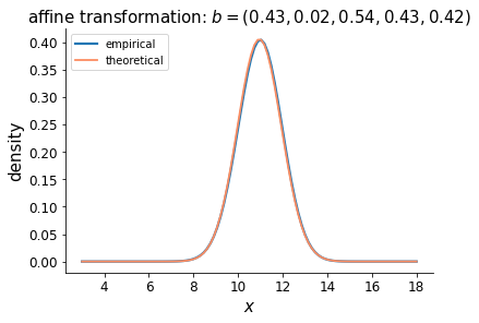
(a)

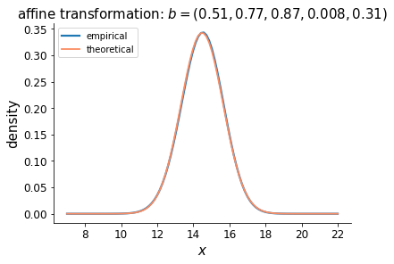
(b)

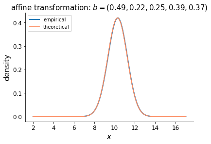
(c)

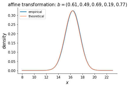
(d)

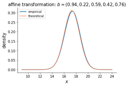
(e)

Figure 9: Distributions after affine transformations

(a)

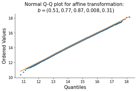
(b)

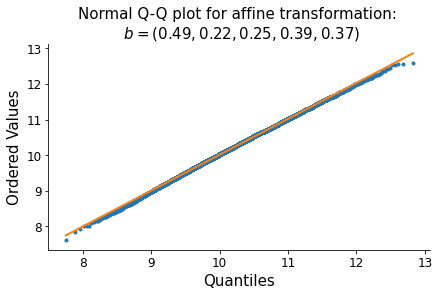
(c)

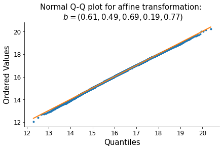
(d)

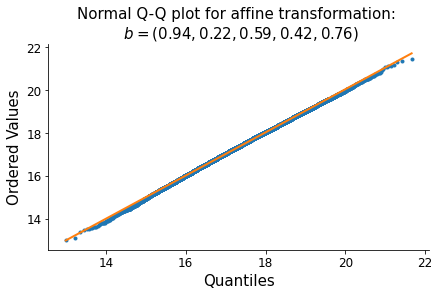
(e)

Figure 10: Normal Q-Q plots after affine transformations

Here, we introduce a loss metric to measure the quality of the dataset $X_{1}$. We will apply 40,000 random affine transformations on the 5-dimensional dataset we got from the Adversarial Network. For each affine transformation, we use the Wasserstein distance to measure the difference between the empirical distribution and the theoretical distribution after the transformation. The Wasserstein distance $W_{p}(P,Q)$ arises from the idea of optimal transport: intuitively, it measures how far you have to move the mass of $P$ to turn it into $Q$. In particular, let $x_{1},...,x_{n}$ be an ordered dataset from the empirical distribution $P$, and $y_{1},...,y_{n}$ be an ordered dataset of the same size from the distribution $Q$, then the distance takes a very simple function of the order statistics: $W_{2}(P,Q)=\left(\sum_{i=1}^{n}||x_{i}-y_{i}||^{2}\right)^{\frac{1}{2}}$. Inspired by this, we use a variation form of the 2-Wasserstein distance as the loss metric: for the $k$-th affine transformation, define the average Wasserstein distance between the empirical distribution and the theoretical distribution as $W(empirical,theoretical)\coloneqq\frac{1}{n}\sum_{i=1}^{n}\frac{1}{\bar{\sigma}_{k}^{2}}||x_{i}-y_{i}||^{2},\forall k\in[1,K]$, where $\bar{\sigma}_{k}$ is the standard deviation of the $k-$th theoretical distribution. In this case, we have $n=$ 20,000 and $K=$40,000. To be specific, for the $k$-th transformation, we get the 20,000 ordered sample points of $X_{1}$ and 20,000 quantiles from the theoretical distribution, then we compute the average Wasserstein distance between the empirical and theoretical distribution. In Figure 11, we show the histogram of the 40,000 average Wasserstein distances after affine transformations.

As a comparison, after each affine transformation, we also generate 20,000 random points from the theoretical distribution. Then we compute the average Wasserstein distances using the 20,000 quantiles from the theoretical distribution and the ordered samples generated from the theoretical distribution. We also present this histogram in Figure 12. We can use this ‘correct answer’ to evaluate the performance in Figure 11.

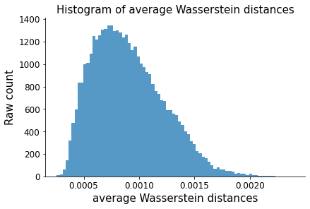
Figure 11: Average Wasserstein distances for the affine transformations of the 5 dimensional samples

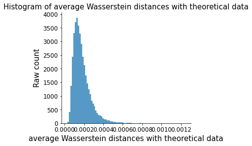
Figure 12: Average Wasserstein distances for the samples generated from theoretical distributions

Finally, we can go further to a $10$-dimensional example, where we set

$x_{0}=\begin{bmatrix}5.0,&5.0,&5.0,&5.0,&5.0,&5.0,&5.0,&5.0,&5.0,&5.0\end{bmatrix}^{\intercal}$ and the terminal distribution

$$\bar{\rho}_{1}=\mathcal{N}\left(\begin{bmatrix}5.5\\ 6.0\\ 5.8\\ 6.0\\ 6.2\\ 5.5\\ 6.0\\ 5.8\\ 6.0\\ 6.2\end{bmatrix},\begin{bmatrix}0.25&0.10&0.10&0.10&0.10&0.10&0.10&0.10&0.10&0.10\\ 0.10&0.25&0.10&0.10&0.10&0.10&0.10&0.10&0.10&0.10\\ 0.10&0.10&0.25&0.10&0.10&0.10&0.10&0.10&0.10&0.10\\ 0.10&0.10&0.10&0.25&0.10&0.10&0.10&0.10&0.10&0.10\\ 0.10&0.10&0.10&0.10&0.25&0.10&0.10&0.10&0.10&0.10\\ 0.10&0.10&0.10&0.10&0.10&0.25&0.10&0.10&0.10&0.10\\ 0.10&0.10&0.10&0.10&0.10&0.10&0.25&0.10&0.10&0.10\\ 0.10&0.10&0.10&0.10&0.10&0.10&0.10&0.25&0.10&0.10\\ 0.10&0.10&0.10&0.10&0.10&0.10&0.10&0.10&0.25&0.10\\ 0.10&0.10&0.10&0.10&0.10&0.10&0.10&0.10&0.10&0.25\end{bmatrix}\right).$$

Using the same network constructed in the $5$-d example, the empirical terminal density $\rho_{1}$ learnt from the Adversarial Network has mean

$\begin{bmatrix}5.4711,&5.9905,&5.8023,&5.9680,&6.2131,&5.4297,&5.9932,&5.7773,&5.9596,&6.1853\end{bmatrix}^{\intercal}$

and covariance matrix

$\begin{bmatrix}0.2522&0.1155&0.1891&0.1305&0.1288&0.1180&0.1016&0.1148&0.1114&0.1217\\ 0.1155&0.2494&0.1346&0.1275&0.0747&0.1170&0.1265&0.0837&0.1217&0.1042\\ 0.1891&0.1346&0.2763&0.1140&0.0939&0.1525&0.1211&0.1417&0.1298&0.0857\\ 0.1305&0.1275&0.1140&0.2622&0.1271&0.1163&0.0892&0.1094&0.1113&0.1067\\ 0.1288&0.0747&0.0939&0.1271&0.1858&0.1325&0.0901&0.0840&0.1120&0.0589\\ 0.1180&0.1170&0.1525&0.1163&0.1325&0.2696&0.1435&0.1121&0.1251&0.1178\\ 0.1016&0.1265&0.1211&0.0892&0.0901&0.1435&0.2578&0.1111&0.0751&0.0843\\ 0.1148&0.0837&0.1417&0.1094&0.0840&0.1121&0.1111&0.2548&0.1076&0.1185\\ 0.1114&0.1217&0.1298&0.1113&0.1120&0.1251&0.0751&0.1076&0.2455&0.0895\\ 0.1217&0.1042&0.0857&0.1067&0.0589&0.1178&0.0843&0.1185&0.0895&0.2368\end{bmatrix}$.

We use a similar way to check the multivariate normality of the empirical distribution. In Figure 13, we plot the marginal distributions of the sample and the target marginal distributions. For most of the margins, the empirical distributions are consistent with the target ones. For margin $5$, we can see the empirical one has a narrower shape (smaller variance), and the empirical margin $6$ is shifted to the left (smaller mean). These imperfectness can also be seen in the mean and covariance matrix of $\rho_{1}$. Then we present the Q-Q plots of the $10$ marginal distributions in Figure 14. Except some outliers at the two ends, the scatters are roughly straight. The Q-Q plots verify that the margins are all normally distributed.

(a) margin 1

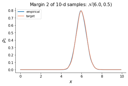
(b) margin 2

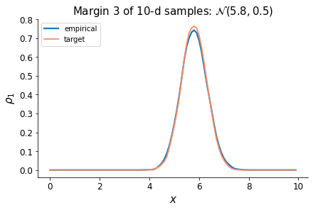
(c) margin 3

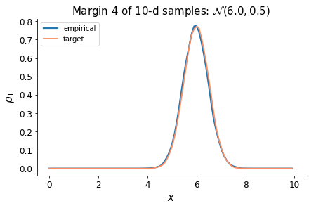
(d) margin 4

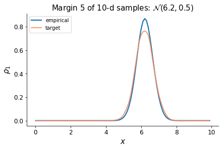
(e) margin 5

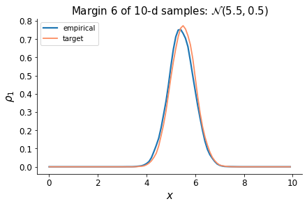
(f) margin 6

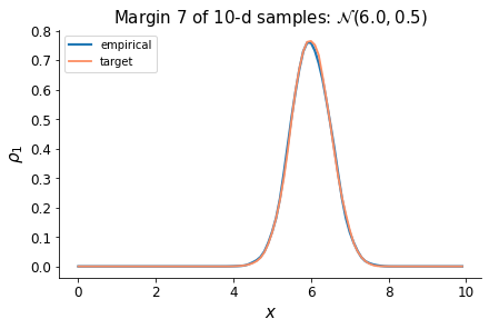
(g) margin 7

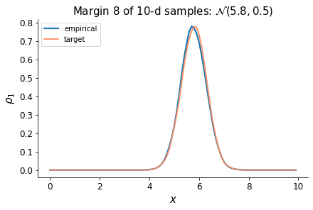
(h) margin 8

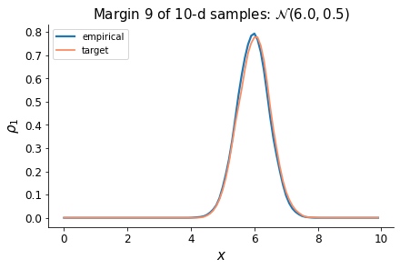
(i) margin 9

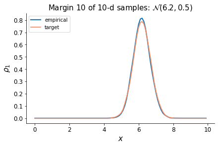
(j) margin 10

Figure 13: Marginal distributions for the 10-d sample

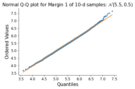
(a) margin 1

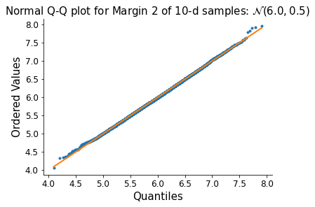
(b) margin 2

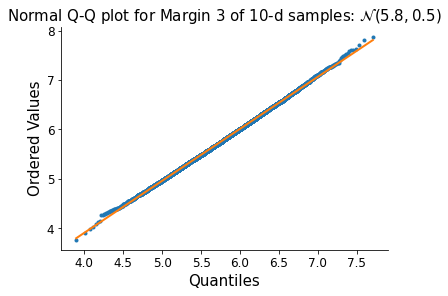
(c) margin 3

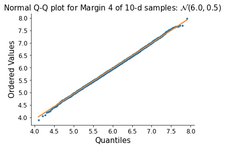
(d) margin 4

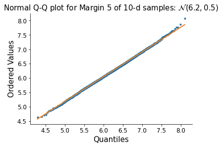
(e) margin 5

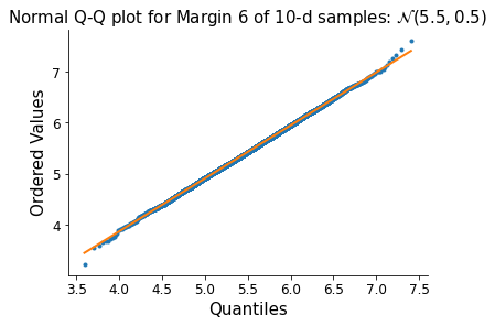
(f) margin 6

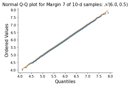
(g) margin 7

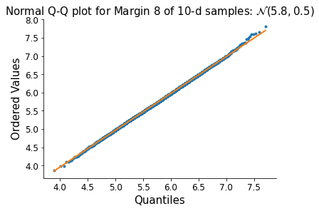
(h) margin 8

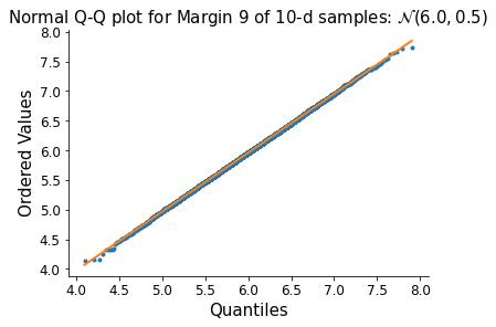
(i) margin 9

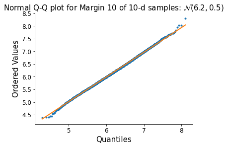
(j) margin 10

Figure 14: Normal Q-Q plots for margins of the 10-d sample

Then, we apply 1,000,000 affine transformations on the 10-dimensional dataset we got from the Adversarial Network. Again, we use the previously defined average Wasserstein distance as a metric to quantify the difference between empirical distribution and the theoretical distribution after the affine transformation. In Figure 15 we plot the histogram of the 1,000,000 average Wasserstein distances for the transformed 10-d samples, and in Figure 16 we illustrate the average Wasserstein distances for the samples generated from theoretical distributions.

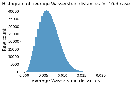
Figure 15: Average Wasserstein distances for the transformed 10-dimensional samples

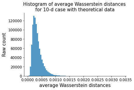
Figure 16: Average Wasserstein distances for the samples generated from theoretical distributions

We want to emphasize that, compared to other research where the prescribed distributions are restricted to Gaussian, our methods apply to a general choice of target distributions $\bar{\rho}_{1}$, such as heavy-tailed and asymmetric distributions. We choose multivariate normal target distributions only because the result is easier to be verified. In the following sections, we will demonstrate examples where $\bar{\rho}_{1}$ is not Gaussian.

5 Application to portfolio allocation

Now we are applying the deep learning algorithm (Algorithm 1) to the portfolio allocation problem introduced in Guo et al. (2020), where the goal is to reach a prescribed wealth distribution $\bar{\rho}_{1}$ at the final time from an initial wealth $x_{0}$. We study this problem with the tools of optimal mass transport.

In this particular application, we consider a portfolio with $d$ risky assets and one risk-free asset, the risk-free interest $r$ being set to 0 for simplicity. We assume the drift $\mu_{t}:\mathcal{E}\rightarrow\mathbb{R}^{d}$ and covariance matrix $\Sigma_{t}:\mathcal{E}\rightarrow\mathbb{S}_{+}^{d}$ of the risky assets are known Markovian processes. The price process of the risky assets is denoted by $S_{t}\in\mathbb{R}^{d}$ $(0\leq t\leq 1)$, and the $i$th element of $S_{t}$ follows the semimartingale

$$\frac{dS_{t}^{i}}{S_{t}^{i}}=\mu_{t}^{i}dt+\sum_{j=1}^{d}\sigma_{t}^{ij}dW_{t}^{j},\quad 1\leq i\leq d,$$ (14)

where $\sigma_{t}\coloneqq\Sigma_{t}^{\frac{1}{2}}\in\mathbb{R}^{d\times d}$ is the diffusion coefficient matrix.

The process $\alpha=(\alpha_{t})_{t\in[0,1]}$ is a Markovian control. For $t\in[0,1]$, the portfolio allocation strategy $\alpha_{t}\in\mathbb{R}^{d}$ represents the proportion of the total wealth invested into the $d$ risky assets, and $1-\sum_{i=1}^{d}\alpha_{t}^{i}$ is the proportion invested in the risk-free asset. We define the concept of admissible control as follows.

Definition 1.

An admissible control process $\alpha$ for the investor on $[0,1]$ is a progressively measurable process with respect to $\mathbb{F}$, taking values in a compact convex set $K\subset\mathbb{R}^{d}$. The set of all admissible $\alpha$ is compact and convex, denoted by $\mathcal{K}$.

We denote by $X_{t}\in\mathbb{R}$ the portfolio wealth at time $t$. Starting from an initial wealth $x_{0}$, the wealth of the self-financing portfolio evolves as follows,

$$dX_{t} =X_{t}\alpha_{t}^{\intercal}\mu_{t}dt+X_{t}\alpha_{t}^{\intercal}\sigma_{t}dW_{t},$$ (15)

$$X_{0} =x_{0}.$$ (16)

In this case, $\rho_{t}\coloneqq\mathbb{P}\circ X_{t}^{-1}\in\mathcal{P}(\mathbb{R})$ is the distribution of the portfolio wealth $X_{t}$. With a convex cost function $F(\alpha_{t}):K\rightarrow\mathbb{R}$, our objective function in this application is

$$\inf_{\alpha,\rho}\left\{\int_{\mathcal{E}}F(\alpha_{t})d\rho(t,x)+C(\rho_{1},\bar{\rho}_{1})\right\},$$ (17)

where the feasible $(\alpha,\rho)$ in (17) should satisfy the initial distribution

$$\rho(0,x) =\rho_{0}(x) \quad\forall x\in\mathbb{R},$$ (18)

and the Fokker–Planck equation

$$\partial_{t}\rho(t,x)+\partial_{x}(\alpha_{t}^{\intercal}\mu_{t}x\rho(t,x))-\frac{1}{2}\partial_{xx}(\alpha_{t}^{\intercal}\Sigma_{t}\alpha_{t}x^{2}\rho(t,x)) =0 \quad\forall(t,x)\in\mathcal{E}.$$ (19)

In the formulation in (15), the drift of the state variable $B(t,x)=\alpha_{t}^{\intercal}\mu_{t}x$ and the diffusion $\mathcal{A}(t,x)=\alpha_{t}^{\intercal}\Sigma_{t}\alpha_{t}x^{2}$. It is easy to check that $\mathcal{A}$ and $B$ are constrained in such a way that $\mathcal{A}\geq\frac{B^{2}}{\left\|\nu_{t}\right\|^{2}}$, where $\nu_{t}\coloneqq\Sigma_{t}^{-\frac{1}{2}}\mu_{t}$. Note that, due to the inequality constraint on the drift and diffusion, not all target distributions are attainable in this application. Therefore, we mainly utilize Algorithm 1 to solve this problem, it can be applied to all types of terminal distributions, attainable or unattainable.

5.1 Numerical Results

Now we implement Algorithm 1 to solve Problem 1 with various penalty functionals. In the experiment, we use $M=512000$ Monte Carlo paths, and $N=64$ time steps. We discretize the time horizon into constant steps with a step size $\Delta t=1/N$ and the spatial domain into $I=100$ constant grids. At each time step, the neural network $\theta_{n}$ consists of 3 layers, with neurons $[60,40,20]$. We feed the neural network with sequential mini-batches of size $1024$ and trained it for $100$ epochs.

5.1.1 Squared Euclidean Distance

In this example, we assume there is one risky asset in the portfolio, i.e., $\alpha_{t}\in\mathbb{R}$. We use the squared Euclidean distance as the penalty functional and a cost function $F(\alpha_{t})=(\alpha_{t}-0.5)^{2}$. The objective function is

$$V(\rho_{0},\bar{\rho}_{1})=\inf_{\alpha}\left\{\mathbb{E}\Bigl{[}\int_{0}^{1}(\alpha_{t}-0.5)^{2}dt\Bigr{]}+\lambda\int_{\mathbb{R}}\frac{1}{2}\left(\rho_{1}(x)-\bar{\rho}_{1}(x)\right)^{2}dx\right\},$$

where we choose $\lambda=3000$, $x_{0}=5$ and $\bar{\rho}_{1}=\mathcal{N}(6,1)$.

The discretized loss function is

$$L=\frac{1}{M}\sum_{m=1}^{M}\left[\sum_{n=1}^{N}\left(\alpha_{n,m}-0.5\right)^{2}\Delta t\right]+\lambda\sum_{i=1}^{I}\frac{1}{2}\left(\tilde{\rho}_{N}(x_{i})-\tilde{\bar{\rho}}_{N}(x_{i})\right)^{2}\Delta x.$$

We compare the KDE-estimated empirical terminal density $\tilde{\rho}_{1}$ with the KDE-estimated target density $\tilde{\bar{\rho}}_{1}$ in Figure 17a; then we also compare $\tilde{\rho}_{1}$ with the true target density $\bar{\rho}_{1}$ in Figure 17b. We can see that the portfolio allocation learned with the deep neural network can successfully steer the density to the prescribed one. We show the change of loss function through the training process in Figure 17c. In training, we use a mini-batch gradient descent algorithm, which is a mix of batch gradient descent and stochastic gradient descent. In each step, it uses one mini-batch to compute the gradient and update the loss function. Therefore, as we can see in Figure 17c, the loss function is not monotonic, but the overall trend is decreasing.

We can see the empirical density $\tilde{\rho}_{1}$ converges to the target $\tilde{\bar{\rho}}_{1}$ after the training. The current result is a trade-off between the cost function in $\alpha_{t}$ and the penalty functional over the terminal densities. In theory, we should set $\lambda=+\infty$ in the penalty functional to make $\rho_{1}=\bar{\rho}_{1}$. Empirically, it is sufficient to set $\lambda$ to be a large number for a similar effect.

The distance between $\tilde{\rho}_{1}$ and $\tilde{\bar{\rho}}_{1}$ comes from the imperfect training of the neural networks. There are two sources of error when we compare $\tilde{\rho}_{1}$ with the true target density $\bar{\rho}_{1}$. One is the imperfectly trained model, and the other is the KDE estimation. To reduce the first kind of error, we can try different hyper-parameters in the neural network, e.g., different mini-batch sizes, different structures of the network, etc. On the other hand, we can reduce the second kind of error by choosing more appropriate kernels and bandwidth $h$ for the KDE method.

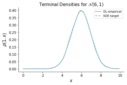
(a) compare $\tilde{\rho}_{1}$ with $\tilde{\bar{\rho}}_{1}$

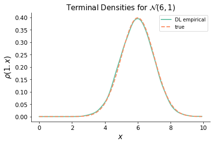
(b) compare $\tilde{\rho}_{1}$ with $\bar{\rho}_{1}$

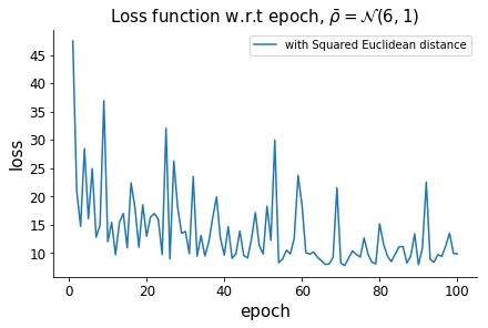
(c) Loss function during the training

Figure 17: Squared Euclidean: $\bar{\rho}=\mathcal{N}(6,1),\lambda=3000,\alpha_{t}\in\mathbb{R}$

An advantage of this deep learning method is that it does not require much extra effort for multi-asset problems. We can easily obtain result for a 4-risky-asset case (or more) with good accuracy within computing time approximately the same as for the 1-risky-asset case. The result for such multi-asset example is shown in Figure 18.

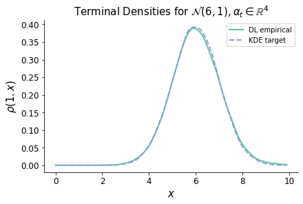
(a) compare $\tilde{\rho}_{1}$ with $\tilde{\bar{\rho}}_{1}$

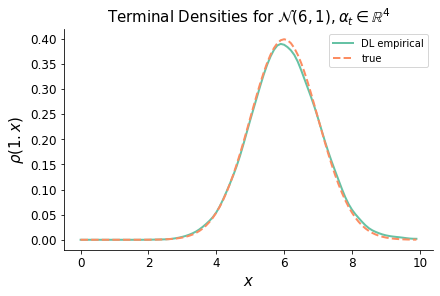
(b) compare $\tilde{\rho}_{1}$ with $\bar{\rho}_{1}$

Figure 18: Squared Euclidean: $\bar{\rho}=\mathcal{N}(6,1),\lambda=3000,\alpha_{t}\in\mathbb{R}^{4}$

5.1.2 Kullback-Leibler divergence

In this second example, we use the Kullback–Leibler divergence to measure the difference between the two distributions. The Kullback–Leibler (K–L) divergence (Kullback and Leibler 1951) is also known as relative entropy or information deviation. In Machine Learning and neuroscience, the K–L divergence plays a leading role and is a widely used tool in pattern recognition (Mesaros et al. 2007), multimedia classification (Moreno et al. 2004), text classification (Dhillon et al. 2003) and so on. In the implementation, we may face $0\log 0$ or division by zero cases in practice; to address this, we can replace zero with an infinitesimal positive value. In this case, the value function is defined as

$$V(\rho_{0},\bar{\rho}_{1})=\inf_{\alpha}\left\{\mathbb{E}\Bigl{[}\int_{0}^{1}(\alpha_{t}-0.5)^{2}dt\Bigr{]}+\lambda\int_{\mathbb{R}}\rho_{1}(x)\log\left(\frac{\rho_{1}(x)}{\bar{\rho}_{1}(x)}\right)dx\right\},$$

and the discretized form of the loss function is

$$L=\frac{1}{M}\sum_{m=1}^{M}\left[\sum_{n=1}^{N}\left(\alpha_{n,m}-0.5\right)^{2}\Delta t\right]+\lambda\sum_{i=1}^{I}\tilde{\rho}_{N}(x_{i})\log\left(\frac{\tilde{\rho}_{N}(x_{i})}{\tilde{\bar{\rho}}_{N}(x_{i})}\right)\Delta x.$$

To show that our method is not restricted to Gaussian target distributions, we use a mixture of two normal distributions as the target $\bar{\rho}_{1}=0.5\mathcal{N}(4,1)+0.5\mathcal{N}(7,1)$ in this example. We provide the comparisons between $\tilde{\rho}_{1}$ and $\tilde{\bar{\rho}}_{1}$, $\tilde{\rho}_{1}$ and $\bar{\rho}_{1}$ in figures 19a and 19b, respectively. The loss function is shown afterwards, in Figure 19c.

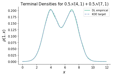
(a) compare $\tilde{\rho}_{1}$ with $\tilde{\bar{\rho}}_{1}$

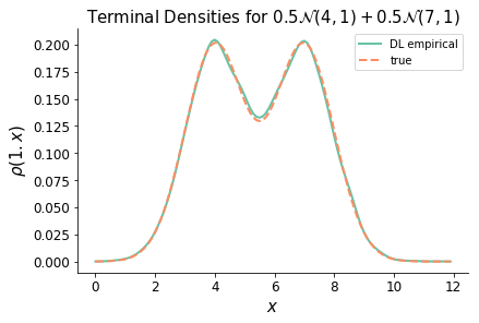
(b) compare $\tilde{\rho}_{1}$ with $\bar{\rho}_{1}$

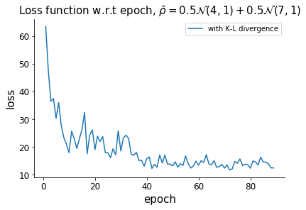
(c) Loss function during the training

Figure 19: K-L divergence: $\bar{\rho}_{1}=0.5\mathcal{N}(4,1)+0.5\mathcal{N}(7,1),\lambda=2000$

We want to emphasize that our method is not restricted to constant parameters. The risky assets can have time-varying returns and covariances. We are not illustrating the results here because the output plots look very similar to the presented cases.

5.1.3 2-Wasserstein Distance

Here, we use 2-Wasserstein distance as the penalty functional. The Wasserstein distance is widely used in Machine Learning to formulate a metric for comparing clusters (Coen et al., 2010), and has been applied to image retrieval (Rubner et al., 2000), contour matching (Grauman and Darrell, 2004), and many other problems. The Wasserstein distance has some advantages compared to distances such as $L^{2},\chi^{2}$ or Hellinger. First of all, it can capture the underlying geometry of the space, which may be ignored by the Euclidean distance. Secondly, when we take average of different objects – such as distributions and images – we can get back to a similar object with the Wasserstein distance. Thirdly, some of the above distances are sensitive to small wiggles in the distribution, but the Wasserstein distance is insensitive to small wiggles.

The 2-Wasserstein distance between two distributions $\rho_{1}$ and $\bar{\rho}_{1}$ is defined by

$$W_{2}(\rho_{1},\bar{\rho}_{1})=\left(\inf_{\gamma\in\Gamma(\rho_{1},\bar{\rho}_{1})}\int_{\mathbb{R}\times\mathbb{R}}\left|x-y\right|^{2}d\gamma(x,y)\right)^{\frac{1}{2}}.$$

For continuous one-dimensional probability distributions $\rho_{1}$ and $\bar{\rho}_{1}$ on $\mathbb{R}$, the distance has a closed form in terms of the corresponding cumulative distribution functions $F(x)$ and $\bar{F}(x)$ (see Rüschendorf 1985 for the detailed proof):

$$W_{2}(\rho_{1},\bar{\rho}_{1})=\left(\int_{0}^{1}\left|F^{-1}(u)-\bar{F}^{-1}(u)\right|^{2}du\right)^{\frac{1}{2}}.$$

Empirically, we can use the order statistics:

$$W_{2}(\rho_{1},\bar{\rho}_{1})=\left(\sum_{i=1}^{n}\left|X_{i}-Y_{i}\right|^{2}\right)^{\frac{1}{2}},$$

where the dataset $X_{1},X_{2},...X_{n}$ is increasingly ordered with an empirical distribution $\rho_{1}$, similarly the dataset $Y_{1},Y_{2},...Y_{n}$ is increasingly ordered with an empirical distribution $\bar{\rho}_{1}$.

Using the same cost function and network structure as before, the numerical results for the densities and loss function are illustrated in Figure 20.

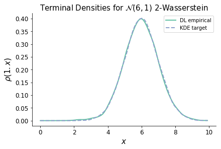
(a) compare $\tilde{\rho}_{1}$ with $\tilde{\bar{\rho}}_{1}$

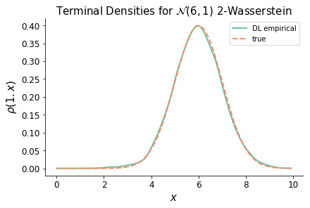
(b) compare $\tilde{\rho}_{1}$ with $\bar{\rho}_{1}$

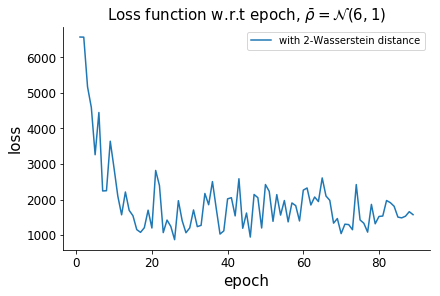
(c) Loss function during the training

Figure 20: 2-Wasserstein distance: $\bar{\rho}_{1}=\mathcal{N}(6,1),\lambda=4000$

6 Conclusion

In this paper, we first devise a deep learning method to solve the optimal transport problem via a penalization method. In particular, we relax the classical optimal transport problem and introduce a functional to penalize the deviation between the empirical terminal density and the prescribed one. In Section 5, we apply this deep learning method to the portfolio allocation problem raised in Guo et al. (2020), where the goal is to reach a prescribed wealth distribution at the final time. We then provide numerical results for various choices of penalty functionals and target densities.

Then we investigate the dual representation and find it can be written as a saddle point problem. In this way, the optimal transport problem can be interpreted as a minimax game between the drift/diffusion and the potential function. We then solve this differential game with adversarial networks. Because this algorithm is free of spatial discretization, it can be applied to high dimensional optimal transport problems, where we illustrate an example up to dimension $10$. These examples validate the accuracy and flexibility of the proposed deep optimal transport method.

References

- Bachouch et al. (2021) Bachouch, A., C. Huré, N. Langrené, and H. Pham (2021). Deep neural networks algorithms for stochastic control problems on finite horizon: numerical applications. Methodology and Computing in Applied Probability. To appear.
- Chen et al. (2019) Chen, L., M. Pelger, and J. Zhu (2019). Deep learning in asset pricing. Available at SSRN 3350138.
- Chow et al. (2019) Chow, Y. T., W. Li, S. Osher, and W. Yin (2019). Algorithm for Hamilton–Jacobi equations in density space via a generalized Hopf formula. Journal of Scientific Computing 80(2), 1195–1239.
- Coen et al. (2010) Coen, M. H., M. H. Ansari, and N. Fillmore (2010). Comparing clusterings in space. In Proceedings of the 27th International Conference on Machine Learning (ICML-10), pp. 231–238.
- Dhillon et al. (2003) Dhillon, I. S., S. Mallela, and R. Kumar (2003). A divisive information-theoretic feature clustering algorithm for text classification. Journal of machine learning research 3(Mar), 1265–1287.
- Eckstein and Kupper (2019) Eckstein, S. and M. Kupper (2019). Computation of optimal transport and related hedging problems via penalization and neural networks. Applied Mathematics & Optimization, 1–29.
- Goodfellow et al. (2014) Goodfellow, I., J. Pouget-Abadie, M. Mirza, B. Xu, D. Warde-Farley, S. Ozair, A. Courville, and Y. Bengio (2014). Generative adversarial nets. In Advances in neural information processing systems, Volume 27, pp. 2672–2680.
- Grauman and Darrell (2004) Grauman, K. and T. Darrell (2004). Fast contour matching using approximate Earth Mover’s Distance. In Proceedings of the 2004 IEEE Computer Society Conference on Computer Vision and Pattern Recognition, 2004. CVPR 2004., Volume 1, pp. I–I. IEEE.
- Guo et al. (2019) Guo, I., N. Langrené, G. Loeper, and W. Ning (2019). Robust utility maximization under model uncertainty via a penalization approach. arXiv preprint arXiv:1907.13345.
- Guo et al. (2020) Guo, I., N. Langrené, G. Loeper, and W. Ning (2020). Portfolio optimization with a prescribed terminal wealth distribution. arXiv preprint arXiv:2009.12823.
- Haber and Horesh (2015) Haber, E. and R. Horesh (2015). A multilevel method for the solution of time dependent optimal transport. Numerical Mathematics: Theory, Methods and Applications 8(1), 97–111.
- Han and E (2016) Han, J. and W. E (2016). Deep learning approximation for stochastic control problems. In NIPS 2016, Deep Reinforcement Learning Workshop.
- Han and Jentzen (2020) Han, J. and A. Jentzen (2020). Algorithms for solving high dimensional PDEs: from nonlinear Monte Carlo to Machine Learning. arXiv preprint arXiv:2008.13333.
- Henry-Labordère (2019) Henry-Labordère, P. (2019). (Martingale) optimal transport and anomaly detection with neural networks: a primal-dual algorithm. Available at SSRN 3370910.
- Huré et al. (2021) Huré, C., H. Pham, A. Bachouch, and N. Langrené (2021). Deep neural networks algorithms for stochastic control problems on finite horizon: convergence analysis. SIAM Journal on Numerical Analysis 59(1), 525–557.
- Huré et al. (2019) Huré, C., H. Pham, and X. Warin (2019). Some machine learning schemes for high-dimensional nonlinear PDEs. arXiv preprint arXiv:1902.01599.
- Kantorovich (1942) Kantorovich, L. V. (1942). On the translocation of masses. In Dokl. Akad. Nauk. USSR (NS), Volume 37, pp. 199–201.
- Kullback and Leibler (1951) Kullback, S. and R. A. Leibler (1951). On information and sufficiency. The Annals of Mathematical Statistics 22(1), 79–86.
- Li et al. (2018) Li, W., E. K. Ryu, S. Osher, W. Yin, and W. Gangbo (2018). A parallel method for Earth Mover’s Distance. Journal of Scientific Computing 75(1), 182–197.
- Liang and Srikant (2016) Liang, S. and R. Srikant (2016). Why deep neural networks for function approximation? arXiv preprint arXiv:1610.04161.
- Loeper (2006) Loeper, G. (2006). The reconstruction problem for the Euler-Poisson system in cosmology. Archive for rational mechanics and analysis 179(2), 153–216.
- McCulloch and Pitts (1943) McCulloch, W. S. and W. Pitts (1943). A logical calculus of the ideas immanent in nervous activity. The Bulletin of Mathematical Biophysics 5(4), 115–133.
- Mesaros et al. (2007) Mesaros, A., T. Virtanen, and A. Klapuri (2007). Singer identification in polyphonic music using vocal separation and pattern recognition methods. In ISMIR, pp. 375–378.
- Monge (1781) Monge, G. (1781). Mémoire sur la théorie des déblais et des remblais. Histoire de l’Académie Royale des Sciences de Paris.
- Moreno et al. (2004) Moreno, P. J., P. P. Ho, and N. Vasconcelos (2004). A Kullback-Leibler divergence based kernel for SVM classification in multimedia applications. In Advances in neural information processing systems, pp. 1385–1392.
- Peyré and Cuturi (2019) Peyré, G. and M. Cuturi (2019). Computational optimal transport: with applications to data science. Foundations and Trends® in Machine Learning 11(5-6), 355–607.
- Rachev and Rüschendorf (1998) Rachev, S. T. and L. Rüschendorf (1998). Mass Transportation Problems: Volume I: Theory, Volume 1. Springer Science & Business Media.
- Rubner et al. (2000) Rubner, Y., C. Tomasi, and L. J. Guibas (2000). The Earth Mover’s Distance as a metric for image retrieval. International journal of computer vision 40(2), 99–121.
- Rüschendorf (1985) Rüschendorf, L. (1985). The Wasserstein distance and approximation theorems. Probability Theory and Related Fields 70(1), 117–129.
- Ruthotto et al. (2020) Ruthotto, L., S. J. Osher, W. Li, L. Nurbekyan, and S. W. Fung (2020). A machine learning framework for solving high-dimensional mean field game and mean field control problems. Proceedings of the National Academy of Sciences 117(17), 9183–9193.
- Santambrogio (2015) Santambrogio, F. (2015). Optimal transport for applied mathematicians. Birkäuser, NY 55(58-63), 94.
- Sirignano and Spiliopoulos (2018) Sirignano, J. and K. Spiliopoulos (2018). DGM: A deep learning algorithm for solving partial differential equations. Journal of Computational Physics 375, 1339–1364.
- Tan and Touzi (2013) Tan, X. and N. Touzi (2013). Optimal transportation under controlled stochastic dynamics. The Annals of Probability 41(5), 3201–3240.
- Villani (2003) Villani, C. (2003). Topics in optimal transportation, Volume 58 of Graduate Studies in Mathematics. American Mathematical Society.
- Villani (2008) Villani, C. (2008). Optimal transport: old and new, Volume 338 of Grundlehren der mathematischen Wissenschaften. Springer Science & Business Media.
- Weinan et al. (2017) Weinan, E., J. Han, and A. Jentzen (2017). Deep learning-based numerical methods for high-dimensional parabolic partial differential equations and backward stochastic differential equations. Communications in Mathematics and Statistics 5(4), 349–380.
- Wiese et al. (2020) Wiese, M., R. Knobloch, R. Korn, and P. Kretschmer (2020). Quant GANs: deep generation of financial time series. Quantitative Finance, 1–22.
- Zhang et al. (2020) Zhang, J., W. Zhong, and P. Ma (2020). A review on modern computational optimal transport methods with applications in biomedical research. arXiv preprint arXiv:2008.02995.
- Zhang et al. (2019) Zhang, K., G. Zhong, J. Dong, S. Wang, and Y. Wang (2019). Stock market prediction based on generative adversarial network. Procedia computer science 147, 400–406.