Polyhedral Lyapunov Functions with Fixed Complexity

Abstract

Polyhedral Lyapunov functions can approximate any norm arbitrarily well. Because of this, they are used to study the stability of linear time varying and linear parameter varying systems without being conservative. However, the computational cost associated with using them grows unbounded as the size of their representation increases. Finding them is also a hard computational problem.

Here we present an algorithm that attempts to find polyhedral functions while keeping the size of the representation fixed, to limit computational costs. We do this by measuring the gap from contraction for a given polyhedral set. The solution is then used to find perturbations on the polyhedral set that reduce the contraction gap. The process is repeated until a valid polyhedral Lyapunov function is obtained.

The approach is rooted in linear programming. This leads to a flexible method capable of handling additional linear constraints and objectives, and enables the use of the algorithm for control synthesis.

I Introduction

In this paper we provide a tool for the analysis and design of Linear Time Varying (LTV) and Linear Parameter Varying (LPV) systems. We first focus on verifying the stability of these systems. Then, we focus on the design of linear feedback for the stabilization problem.

For the stability problem we adopt the framework of polyhedral Lyapunov functions [3]. Those are asymmetric norms (finitely valued, satisfy the triangle inequality, positively homogeneous, and positive definite) whose unit balls are polyhedra. We provide the necessary background on polyhedra and polyhedral Lyapunov functions in Section II, and show how to use them for verifying stability in Section III.

The polyhedral Lyapunov framework is less conservative than standard quadratic Lyapunov functions. But this comes at a price: whereas finding a quadratic Lyapunov function to assess stability is a convex problem, efficiently solved using linear matrix inequalities [4], the same problem is hard to solve for polyhedral Lyapunov functions. In this paper we tackle the problem by developing an approach based on a two step iterated procedure, along the lines of [11]. Each step is a linear program (LP) and the iterations build a sequence of polyhedral sets, each reducing the gap to a contractive set, i.e. to a decaying Lyapunov function. The full algorithm is presented in Section IV.

A relevant feature of our algorithm is that we fix the complexity of the polyhedral Lyapunov function, that is, the number of vertices or constraints that define the polyhedral set. This is one of the features that distinguish our approach from others available in the literature [2, 3, 10, 14, 17]. We provide a comparison in Section VI.

Another relevant feature is that we can easily extend the framework to include additional constraints and new variables, which is of practical significance for control synthesis. This allows us to develop most of our discussion for autonomous linear systems, simplifying the exposition. We then show how the algorithm is generalized to control design and nonlinear systems in Section V. We also show how our algorithm can be used to assess contraction/incremental stability of a system. The effectiveness of the algorithm is illustrated on a DC motor example, in Section VII.

II Mathematical Preliminaries

II-A Polyhedra

We use $\mathcal{C}$ to denote a convex set and $\operatorname{int}\mathcal{C}$ to denote its interior, which we define as the largest open subset of $\mathbb{R}^{n}$ in $\mathcal{C}$. Inequalities on vectors and matrices are used in the element-wise sense. We represent polyhedra in two ways:

given $n\times m$ matrix $V$,

$$\mathcal{C}_{\mathcal{V}}(V)=\{x:x=Vp,\,p\geq 0,\,1^{T}p=1\}$$ (1)

given $m\times n$ matrix $H$,

$$\mathcal{C}_{\mathcal{H}}(H)=\{x:Hx\leq 1\}$$ (2)

For this paper we exclusively use V-representation polyhedra. All results can be readily extended to H-representation polyhedra by duality, [3, Proposition 4.35]. Geometrically, the columns of the $V$ correspond to the vertices of $\mathcal{C}_{\mathcal{V}}(V)$, which is formed by taking their convex hull.

We make the standing assumptions that our polyhedra

$$\bullet\text{ are Bounded}$$ (A1)

$$\bullet\text{ contain $0$ in their interior}$$ (A2)

Assumption (A1) is always true for V-representation polyhedra. Eq. (A2) requires that there exists a $p_{+}>0$ such that $0=Vp_{+}$, which we can test using linear programming (LP).

II-B Polyhedral Lyapunov Functions

Any convex set $\mathcal{C}$ defines a non-negative function through its Minkowski functional. The Minkowski functional of a set $\mathcal{C}$ is given by

$$\Psi_{\mathcal{C}}(x)=\inf\{r\in\mathbb{R}:r>0\text{ and }x\in r\mathcal{C}\}$$ (3)

For V-representation polyhedra this means

$$\Psi_{V}(x)=\min\{1^{T}p\,:\,x=Vp,\,p\geq 0\}$$ (4)

Using the strong duality of LP problems [5, Section 5.2.1], this is equivalent to

$$\Psi_{V}(x)=\max\{h^{T}x\,:\,h^{T}V\leq 1^{T}\}$$ (5)

Using LP, (4) and (5) can be evaluated numerically at any given point. For V-representation polyhedra satisfying (A2), $\Psi_{V}$ is always a real valued function, strictly positive for all $x\neq 0$, and radially unbounded. As such they are valid Lyapunov function candidates.

However, for us to fully establish the link with Lyapunov theory we also require the notion of a derivative of the candidate function. Unfortunately, the Minkowski functionals of polyhedra are not everywhere differentiable and we need to resort to the more general setting of subdifferentials:

$$\partial\Psi(x)=\{h\,:\,\forall y\in\mathbb{R}^{n},\,\Psi(y)-\Psi(x)\geq h^{T}(y-x)\}$$ (6)

For differentiable functions the subdifferential at $x$ corresponds to the gradient.

For Minkowski functionals of V-representation polyhedra, we can obtain an explicit representations of $\partial\Psi_{V}(x)$.

Proposition 1 (V-representation Subdifferential)

For any given matrix $V$, consider the Minkowski functional $\Psi_{V}$. Then,

$$\partial\Psi_{V}(x)=\{h\,:\,h^{T}x=\Psi_{V}(x),\,h^{T}V\leq 1^{T}\}$$ (7)

Proof:

$\eqref{eq:subdiff_v}\subseteq\partial\Psi_{V}(x)$: We need to show that $\Psi_{V}(y)\geq h^{T}y$. From (5), this must be true.

$\partial\Psi_{V}(x)\subseteq\eqref{eq:subdiff_v}$: We prove this in two steps. We first show that any $h\in\partial\Psi_{V}(x)$ must satisfy $h^{T}V\leq 1^{T}$ by contradiction. If $h$ doesn’t satisfy $h^{T}V\leq 1^{T}$, there must exist a column of $V$, $[V]_{i}$, such that $h^{T}[V]_{i}=c>1$ and $\Psi_{V}([V]_{i})=1$. If we set $y=k[V]_{i}$, for $h\in\partial\Psi_{V}(x)$ we must then have $k-\Psi_{V}(x)\geq kc-h^{T}x$ for all $k>0$. However, if we set $k>\max(0,(h^{T}x-\Psi_{V}(x))/(c-1))$ the inequality is invalidated, leading to a contradiction. As such, if $h\in\partial\Psi_{V}(x)$ then $h^{T}V\leq 1^{T}$. If we set $y=0$ we get $h^{T}x\geq\Psi_{V}(x)$. But from before $h^{T}V\leq 1^{T}$, and so $h$ must be included in the domain of (5) and therefore $h^{T}x=\Psi_{V}(x)$. Since $h$ satisfies both $h^{T}V\leq 1^{T}$ and $h^{T}x=\Psi_{V}(x)$, $h\in\eqref{eq:subdiff_v}$. ∎

We use subdifferentials to quantify how our candidate Lyapunov function $\Psi_{V}$ changes along system trajectories.

Proposition 2

For any trajectory $x(\cdot)$ of the autonomous system $\dot{x}=Ax$,

$$\Psi_{V}(x(t))-\Psi_{V}(x(0))=\int_{0}^{t}\sup_{h\in\partial\Psi_{V}(x(\tau))}h^{T}Ax(\tau)d\tau$$ (8)

Proof:

See [6] and [3, Sections 2.2]. ∎

The integrand is equivalent to $\max h^{T}Ax$ subject to $h^{T}x=\Psi_{V}(x),\,h^{T}V\leq 1^{T}$, which is an LP that we can directly numerically compute.

III Contraction, Linear Programming,
and Lyapunov Stability

Convex sets can be used to show stability through the notion of contraction (also frequently referred to as strict positive invariance). For continuous time systems, this requires us to first define tangent cones. For a general convex set $\mathcal{C}$, the interior of the tangent cone at a point $x\in\mathcal{C}$ is given by

$$\operatorname{int}\mathcal{K}_{\mathcal{C}}(x)=\{w\,:\,\lambda>0,\,x+\lambda w\in\operatorname{int}\mathcal{C}\}$$ (9)

We then say that $\mathcal{C}$ is a contracting convex set under the dynamics $\dot{x}=Ax$ if

$$\forall x\in\mathcal{C},\,Ax\in\operatorname{int}\mathcal{K}_{\mathcal{C}}(x)$$ (10)

This can be interpreted in words as saying that the flow induced by the dynamics maps all points in $\mathcal{C}$ to points in $\operatorname{int}\mathcal{C}$ for all $t>0$. For polyhedra, we can express this geometric condition in a more convenient form.

Proposition 3 (Contraction in V-representation)

For a polyhedron $\mathcal{C}_{\mathcal{V}}(V)$, (10) is equivalent to $\exists M\in\mathbb{R}^{m\times m}$ and scalar $\eta>0$ such that

$$-\eta 1^{T} =1^{T}M,$$ (11a)

$$AV =VM,$$ (11b)

$$\operatorname{off-diag}(M) \geq 0\text{ [$\equiv M$ is Metzler]}$$ (11c)

Where we use $\operatorname{off-diag}(M)\geq 0$ to denote that all elements of $M$ outside of the main diagonal are non-negative. We call $\eta$ the rate of contraction.

Proof:

For $\mathcal{C}_{\mathcal{V}}(V)$, we use (1) to express (10) as

$$\forall (p\geq 0,1^{T}p=1):$$

$$\exists (\lambda>0,\hat{p}\geq 0,1^{T}\hat{p}<1):AVp=\lambda^{-1}V(\hat{p}-p)$$

This is equivalent to

$$\exists(\Lambda>0,\hat{P}\geq 0,1^{T}\hat{P}<1^{T}):AV=V\Lambda^{-1}(\hat{P}-I)$$

where $\Lambda$ is a diagonal matrix. Setting $\hat{M}=\Lambda^{-1}(\hat{P}-I)$, we rewrite this as:

$$\exists(\eta>0,\hat{M}):1^{T}\hat{M}\leq-\eta 1^{T},AV=V\hat{M},\operatorname{off-diag}(\hat{M})\geq 0$$

From (A2), $\exists p_{+}>0$ such that $0=Vp_{+}$. We can then add this $p_{+}$ to each column of $\hat{M}$ until it satisfies (11a) without affecting (11b) or (11c). ∎

Testing contraction is thus an LP optimization problem.

$$\max_{M,\eta}\, \eta$$ (12)

s.t.: $$\eqref{eq:contracting}$$

The conditions of Proposition 3 are verified if the maximization in (12) is greater than $0$.

It is fairly straightforward to show that set contraction implies stability through the homogeneity of the linear dynamics. However, using (7), we can build a direct connection to Lyapunov theory.

Proposition 4 (Lyapunov stability)

$\mathcal{C}_{\mathcal{V}}(V)$ is a contracting set for $A$ with rate $\eta$ if and only if

$$\forall x\in\mathbb{R}^{n}\quad\sup_{h\in\partial\Psi_{V}(x)}h^{T}Ax\leq-\eta\Psi_{V}(x)$$ (13)

Proof:

(11) $\implies$ (13): Starting with (7) and (4) we have that there exists some $p$ such that $h^{T}x=1^{T}p=\Psi_{V}(x),\,x=Vp,\,p\geq 0$ for the $h\in\partial\Psi_{V}(x)$ that maximizes $h^{T}Ax$. Also note that we can rewrite a matrix $M$ satisfying (11c) as $M=P+\delta I$, where $P$ is an positive matrix. Therefore

$$h^{T}Ax =h^{T}AVp$$

$$=h^{T}VMp\quad\eqref{eq:contracting_equality_main}$$

$$=h^{T}V(P+\delta I)p=h^{T}VPp+\delta h^{T}Vp$$

$$=h^{T}VPp+\delta 1^{T}p\quad[x=Vp,\,1^{T}p=h^{T}x]$$

$$\leq 1^{T}Pp+\delta 1^{T}p=1^{T}Mp\quad\text{[$h\in\partial\Psi_{V}(x),\,Pp\geq 0$]}$$

$$\leq-\eta 1^{T}p\quad\eqref{eq:contracting_rate}$$

$$\leq-\eta\Psi_{V}(x)$$

(13) $\implies$ (11): We show this by contradiction. The optimization problem in (11) can be broken down to multiple multiple sub-problems, one for each column of $V$, $[V]_{i}$:

$$\exists p\in\mathbb{R}^{m}\,:\,\eta=-1^{T}p,\,A[V]_{i}=Vp,\,p_{j\neq i}\geq 0$$ (14)

where $\{j\neq i\}$ is $[1,m]\setminus\{i\}$. If (11) is infeasible for a given $\eta$ then (14) must be infeasible for at least one $[V]_{i}$. This is because otherwise a feasible solution for (11) could be generated by aggregating $\{p\}$ into a matrix $P$. As such we begin by assuming that there exists some $[V]_{i}$ for which (14) is infeasible. Then, by Farkas’ Lemma, there exists an $h$ such that

$$h^{T}A[V]_{i}>-\eta,\,h^{T}[V]_{i}=1,\,h^{T}V\leq 1^{T}$$ (15)

This means that $h\in\partial\Psi_{V}([V]_{i})$. But, since, $\Psi_{V}([V]_{i})=1$, $h^{T}A[V]_{i}>-\eta\Psi_{V}([V]_{i})$, contradicting (13). ∎

From Lyapunov theory, (13) with $\eta>0$ combined to (8) imply global exponential stability of the system with convergence rate $\eta$. The connection between contraction and Lyapunov stability is a well-known result in system theory [3, Thm 4.24, 4.33]. However, we include this proof to show how we can use (7) to directly proof results about polyhedral Lyapunov functions. We hope to use this approach to extend results that have no direct interprettation as set contraction, such as dissipativity, to polyhedral Lyapunov functions. This can be particularly useful for control design and for the analysis of open systems.

IV Algorithm for Finding Polyhedra

IV-A Overview

Testing if a set is contracting under the linear dynamics $\dot{x}=Ax$ is a much easier problem than finding a contractive set. In fact, treating $V$ as a variable makes (11b) nonconvex and nonlinear (since $M$ and $\eta$ are also variables). However, we can instead try to find such a $V$ iteratively, by decomposing (12) into a pair of LP problems. One considers $V$ fixed and estimates the contraction gap of $V$. The other, introduces variations on $V$ to reduce the contraction gap.

To initialize our algorithm we need to build an initial candidate polyhedron which satisfies our standing assumptions. A possible construction is suggested in Remark 1. The number of vertices $m$ of our polyhedron will remain the same throughout the whole procedure. This means that we can control the complexity of our Lyapunov function and treat $m$ as an input parameter.

(i) Estimation of the contraction gap: for any given candidate polyhedron $V$, the contraction gap is estimated via the LP optimization (12) The following Proposition justifies the use of (12).

Proposition 5

Given a $\mathcal{C}_{\mathcal{V}}(V)$ that satisfies (A2), there exists some finite $\eta$ (not necessarily $>0$) that satisfies (11). Additionally, if $\mathcal{C}_{\mathcal{V}}(V)$ satisfies (11) for some $\eta^{*}$, it will also satisfy (11) for any $\eta<\eta^{*}$.

Proof:

Note that (A2) implies that $V$ is full row rank since otherwise the strict interior of $\mathcal{C}_{\mathcal{V}}(V)$ would be empty. We rewrite $p=p_{b}+\delta_{i}p_{+}$, where $p_{b}$ is a solution to $A[V]_{i}=Vp_{b}$ (implied to exist because $V$ is full row rank) and $p_{+}>0$ is a positive solution to $0=Vp_{+}$ (implied to exist because of (A2)). There then exists a $\delta_{i}^{*}$ such that $A[V]_{i}=Vp$ and $p_{i\neq j}\geq 0$ for all $\delta_{i}\geq\delta_{i}^{*}$. Since $1^{T}p_{+}>0$, increasing $\delta_{i}$ decreases $\eta_{i}=-1^{T}p_{b}-\delta_{i}1^{T}p_{+}$. As such, there exists $\{\delta_{i}\}$ such that for all $i$ $\eta_{i}^{*}=-\min_{i}\{1^{T}p_{b}+\delta_{i}^{*}p_{+}\}$. Aggregating $\{p\}$ into a matrix $P$ produces a solution to (11) with $\eta=\eta_{i}^{*}$. By increasing $\{\delta_{i}\}$ further, (11) can be satisfied for any $\eta<\eta^{*}$. ∎

If $\eta>0$ we conclude that our polyhedron is contracting and we are done.

(ii) Reduction of the contraction gap: if $\eta\leq 0$, the following LP program searches for variations on $V$ that are compatible with a reduction of the contraction gap. For a small $\varepsilon>0$, solve:

$$\max_{\delta\eta,\delta M,\delta V}\, \>\delta\eta$$ (16a)

$$-\delta\eta 1^{T} =1^{T}\delta M,$$ (16b)

$$A\delta V =\delta VM+V\delta M,$$ (16c)

$$0 \leq\operatorname{off-diag}(M+\delta M)$$ (16d)

$$\|\delta V\|_{1} \leq\varepsilon,\,\|\delta M\|_{1}\leq\varepsilon$$ (16e)

The idea is to look for variations $\delta V$ in a small neighborhood of $V$ that would improve the gap $\eta<\eta+\delta\eta$. The search space is limited to the tangent space of the constraints manifold, at the point $(\eta,V,M)$. Therefore, for small enough variations, any solution to the LP above improves the contraction rate while preserving the integrity of the constraints. We thus build the new polyhedron as $V_{\textrm{new}}:=V+\delta V$. A small $\varepsilon$ ensures that the $V_{\textrm{new}}$ remains in a small neighborhood of $V$ to be compliant with the linear approximation above. It also guarantees that $\mathcal{C}_{\mathcal{V}}(V_{\textrm{new}})$ satisfies our standing assumption (by continuity argument).

The procedure iterates between these two steps until the estimation of the contraction gap returns a positive $\eta$.

Remark 1

We compute an initial candidate polyhedron by randomly sampling $m-1$ points in $\mathbb{R}^{n}$ and rescaling them to have length 1. We then add an additional vertex equal to minus their sum and again normalised to have length 1. This way we obtain a polyhedron $\mathcal{C}_{\mathcal{V}}(V)$ with $m$ irreducible vertices that, as long as $m\geq n+1$, must also satisfy (A2).

IV-B Fast reduction of the contraction gap

We can speed up (16) by not having $\delta\eta$ and $\delta M$ as variables in the second optimization problem. We do this by considering directions in the tangent space that are compatible with the optimality conditions of (12) around a fixed previous solution. With these extra restrictions in place, we can obtain a directional derivative of $\eta$ with respect to $V$.

To estimate this derivative we need to rewrite (12) into standard LP form

$$\max_{\hat{x}}\, \>\hat{c}^{T}\hat{x}$$ (17a)

s.t.: $$\hat{A}\hat{x} =\hat{b}$$ (17b)

$$\hat{x} \geq 0$$ (17c)

where $\hat{A}$ is a $k\times l$ matrix. A detailed transformation procedure is provided in Section IV-C.

Using the standard form, we can then make use of the notion of Basic Feasible Solutions (BFS): from [15, Section 13.2], a BFS of (17) is a set $\mathcal{B}\subset\{1,..,l\}$ and a vector $\hat{x}$ such that:

• $\hat{A}\hat{x}=\hat{b}$ and $\hat{x}\geq 0$

• $\mathcal{B}$ contains $k$ elements

• $i\not\in\mathcal{B}\implies\hat{x}_{i}=0$.

• The $k\times k$ matrix $\hat{B}$ defined as

  $$\hat{B}=[\hat{A}_{i}]_{i\in\mathcal{B}}$$

  is non-singular, where $\hat{A}_{i}$ is the $i$th column of $\hat{A}$.

When solving (17) it is sufficient to only consider BFSs [15, Theorem 13.2]. We can obtain a BFS that is also an optimal solution of (17) via the Simplex algorithm [7]. Many commercial interior point solvers also offer the option of deriving a BFS as a cheap post-processing stage.

With the optimal BFS we can now find the derivative of $\eta$ with respect to changes in $V$. In general, we need to implicitly differentiate equation (17b) to obtain a derivative of $\hat{x}$ (which represents our variables $\eta$ and $M$ in standard form) with respect to $\hat{A}$ and $\hat{b}$ (which are functions of $V$). However, an explicit solution can only be obtained if $\hat{A}$ is invertible [8]. Instead, we restrict ourselves to the BFS and consider only variables that aren’t constrained to be $0$ by our choice of $\mathcal{B}$. Indeed, given $\hat{y}=\{\hat{x}_{i}:i\in\mathcal{B}\}$, we can always obtain the derivative of $\hat{y}$ with respect to $\hat{B}$ and $\hat{b}$. Because $\hat{B}$ is invertible (from the properties of the BFS), this derivative is always well defined.

Using the transformation in Section IV-C, we can map the LP problem back to its original coordinates and build an explicit representation of $D_{V}\eta$ and $D_{V}M$. We can then replace (16) with the following LP optimization problem:

$$\max_{\delta V}\, (D_{V}\eta)(\delta V)$$ (18)

subject to: $$\|\delta V\|_{1}\leq\varepsilon$$

$$\text{and}: \quad\operatorname{off-diag}(M+ (D_{V}M)(\delta V))\geq 0$$

By constraining $\delta V$ to be small enough we can also ensure that the new polyhedron $\mathcal{C}_{\mathcal{V}}(V+\delta V)$ satisfies (A1) and (A2). This can also be enforced directly, as in [11], but keeping $\delta V$ small seems to work sufficiently well in practice.

We summarize the full algorithm below:

Data: The matrix $A$, the maximum number of iterations,
and the number of vertices in the matrix $m$
Result: $V$ satisfying (11) if found, else $False$
Procedure:
$V^{(0)}=$ Initialize$(m)$
$k=0$
while $k\leq\texttt{max\_iter}$:
     $\eta,M,\mathcal{B}=$ Optimal BFS of (12) with $V=V^{(k)}$
     if $\eta>0$:
        return $V^{(k)}$
     $D_{V}\eta,D_{V}M\!=\!$ Derivatives of (12) using $\mathcal{B}$ and $V\!=\!V^{(k)}$
     $\delta V=$ (18) using $M,\,D_{V}\eta,$ and $D_{V}M$
     $V^{(k+1)}=V^{(k)}+\delta V$
     $k:=k+1$
return $False$

Algorithm 1 Stability Verification Algorithm

IV-C The Derivative Computation in Detail

To go from (12) to (17) we use the vectorization operator $\operatorname{vec}(\cdot)$, which converts a $n\times m$ matrix into a column vector with $nm$ entries by stacking up its columns and the Kronecker product ($\otimes$):

$$\hat{A}= \begin{bmatrix}I_{m}\otimes V&-\operatorname{vec}(V)&0_{nm}&0_{nm}\\ I_{m}\otimes 1_{m}^{T}&-1_{m}&1_{m}&-1_{m}\end{bmatrix} \quad\hat{b}= \begin{bmatrix}\operatorname{vec}(AV)\\ 0_{m}\end{bmatrix}$$

$$\hat{c}= \begin{bmatrix}0_{mm}\\ 0\\ 1\\ -1\end{bmatrix} \quad\hat{x}= \begin{bmatrix}\operatorname{vec}(P)\\ -\delta\\ \eta_{+}\\ \eta_{-}\end{bmatrix}$$ (19)

where $\eta_{+}-\eta_{-}=\eta$ and $P+\delta I=M$. We can also rewrite (17b) as

$$f=\hat{A}\hat{x}-\hat{b}=\hat{B}\hat{y}-\hat{b}=\hat{G}\operatorname{vec}(V)=0$$ (20)

where

$$\hat{G}=\begin{bmatrix}M^{T}\otimes I_{n}-I_{m}\otimes A\\ 0_{m\times(nm)}\end{bmatrix}$$ (21)

From (20), we use the implicit function theorem to compute the Jacobian of $\hat{y}$ with respect to $\operatorname{vec}(V)$

$$\nabla_{\operatorname{vec}(V)}\hat{y}=-(\nabla_{\hat{y}}f)^{-1}\nabla_{\operatorname{vec}(V)}f=-\hat{B}^{-1}\hat{G}$$ (22)

such that $(D_{V}\hat{y})(\delta V)=(\nabla_{\operatorname{vec}(V)}\hat{y})\operatorname{vec}(\delta V)$.

For our derivatives of interest

$$(D_{V}\eta)(\delta V)=(D_{V}\eta_{+})(\delta V) -(D_{V}\eta_{-})(\delta V)$$

$$\text{and, }\forall i\neq j,\,(D_{V}M_{ij})(\delta V) =(D_{V}P_{ij})(\delta V)$$

Note that all derivatives on the right hand side are of elements of $\hat{x}$. To compute each of them we first obtain the corresponding index $i$ in $\hat{x}$ from (19). Then, if $i\not\in\mathcal{B}$, the derivative is zero. Else, we obtain the corresponding index $j$ in $\hat{y}$ so that $\hat{x}_{i}=\hat{y}_{j}$. To compute the derivative, we then multiply the $j^{th}$ row of (22) with $\operatorname{vec}(\delta V)$.

Our derivative calculations can be interpreted as only considering the effect of changes in $V$ to our variables under a fixed basis. As long as the solution with the current basis is feasible for $V+\delta V$, this will still be a BFS (although it might not be the optimal one).

V Generalizations

V-A Feedback Design

Algorithm 1 can be readily extended for output-feedback design for systems of the form

$$\dot{x}=Ax+Bu\qquad\quad y=Cx.$$

This includes state feedback as a special case when $C=I$. We replace (12) with

$$\max_{M,K,\eta}\, \eta$$ (23)

s.t.: $$-\eta 1^{T} =1^{T}M,$$

$$(A+BKC)V =VM,$$

$$\operatorname{off-diag}(M) \geq 0\text{ [$\equiv M$ is Metzler]}$$

The two step procedure outlined in Section IV reduces the nonlinear (for non-fixed $V$) program (12) into an iteration involving linear programs. A similar reduction can be applied to (23). Just like (12), (23) is a linear program for fixed $V$, which means that the estimation of the contraction gap is a straightforward operation. Likewise, for (23), the reduction of contraction gap step is performed on a larger manifold, which now also contains $K$. However, the search procedure remains essentially the same. This means that the approach in (IV-B) can also be adapted to control synthesis (it just requires different transformations to get the constraints into standard form).

We can also consider scenarios beyond simple stabilization. New formulations may be considered as long as they are encoded into linear constraints. Natural directions to explore are testing/enforcing input/output gains, the design of dynamic output feedback, and the design of nonlinear state-feedback controllers taking advantage of the Lyapunov framework. This will be the goal of future research.

V-B From Linear Stability to LDIs

The discussion in this paper has been developed for simple linear systems but, since (12) and (23) are convex, the same approach can be used for the analysis LTV and LPV systems, and even for nonlinear systems.

The idea is that systems of the form

$$\dot{x}=A(w(t))x+B(w(t))u$$ (24)

satisfy, for all $t\geq 0$,

$$A(w(t))\in\operatorname{ch}\{A_{i}\},\,B(w(t))\in\operatorname{ch}\{B_{i}\}$$

where

$$\operatorname{ch}\{A_{i}\}=\{A:A=\sum_{i}p_{i}A_{i},\,p_{i}\geq 0,\,\sum_{i}p_{i}=1\};$$

and likewise for $\operatorname{ch}\{B_{i}\}$.

Stability is thus verified as in (12) where constraints (11a) and (11b) are replaced by several constraints of the form

$$-\eta 1^{T}=1^{T}M_{i}\text{ and }A_{i}V=VM_{i}\ .$$

Indeed, the extension of the constraint set does not change the structure of the solution. Combined with (23), this allows us to tackle the design of a stabilizing linear state-feedback law $u=Kx$.

A similar approach can be explored to verify contraction [12, 18, 16, 9] of nonlinear systems of the form $\dot{x}=f(x)$. The problem reduces to finding a contracting polyhedral set $V$ for the linearization

$$\dot{\delta x}=\partial f(x)\delta x\qquad\quad\forall x\ .$$

The solution is obtained as above, by relaxing the problem to a suitable convex hull $\partial f(x)\in\operatorname{ch}\{A_{i}\}$ for all $x$.

VI Comparison with Related Approaches

In systems theory polyhedral Lyapunov functions are usually constructed using algorithms that progressively add new vertices or constraints until a contractive set is reached. Other algorithms exploit optimization based approaches to directly construct contractive sets.

[3], [10] and [14] provide examples of the iterative approach. The new vertices are generated by iterating the update equation of discrete-time linear systems. The main advantage of these approaches is that in many cases the sequence of polyhedra produced can be guaranteed to converge to a polyhedral Lyapunov function, if one exists. The main disadvantage is that not all linear constraints can be incorporated easily. Additionally, it is difficult to bound the complexity of the resulting polyhedron.

Examples of optimization-based algorithms can be found in [2] and [17]. [17] considers positive rescalings of the vertices of the initial candidate polyhedron. This allows for fast computation but may lead to high complexity polyhedra even when a simple contractive polyhedron exists. The algorithm in [2] makes clever use of both representations of a polyhedron. However, this is also a limiting factor because of the possible difference in the number of vertices and constraints of the two representations. In higher dimensions, a few vertices/constraints in one representation may lead to a very large number of constraints/vertices in the other representation [13], which hinders the use of the algorithm in high dimensional settings.

The approach proposed in this paper is also optimization-based. It takes into account explicitly the problem of complexity of the polyhedron by taking the number of vertices of the polyhedron as a parameter. This comes at the price of weaker convergence guarantees (if the predefined number of vertices is too small the problem is unfeasible). Our algorithm generalizes the approach of [17] by allowing vertices to move freely, and, in constrast to [2], only uses a single representation. Our approach also tackles the problem linear control synthesis which is not considered by any of the approaches above.

VII Example: DC Motor

We test our optimization-based approach on the DC motor speed and position examples from [1]. For the DC motor speed example, we carry out a stability analysis under various possible parameter variations. We then solve the feedback design problem for the DC motor position example using both static and dynamic state feedback. We use the parameters given in the website for the speed example as our nominal values throughout (inertia $J_{0}=.01$, viscous friction constant $b_{0}=.1$, emf constant $K_{0}=.01$, resistance $R_{0}=1$, and inductance $L_{0}=.5$).

The DC motor speed example is governed by the following dynamics:

$$\frac{d}{dt}\begin{bmatrix}\omega\\ i\end{bmatrix}=\begin{bmatrix}-b/J&K/J\\ -K/L&-R/L\end{bmatrix}\begin{bmatrix}\omega\\ i\end{bmatrix}$$ (25)

In this case, we consider 2 orders of magnitude of parameter perturbations of the form

$$J\in[J_{0}/\gamma_{s},\gamma_{s}J_{0}],\,b\in[b_{0}/\gamma_{s},\gamma_{s}b_{0}],\,K\in[K_{0}/\gamma_{s},\gamma_{s}K_{0}]$$ (26)

for $\gamma_{s}=10$. Using Algorithm 1, we are able to find a polyhedron satisfying (13) and (26) (with $\eta=.07$). It is shown in Fig. 1 and has only 6 vertices. For comparison, we are only able to find a common quadratic function using LMIs up to around $\gamma_{s}=8.7$.

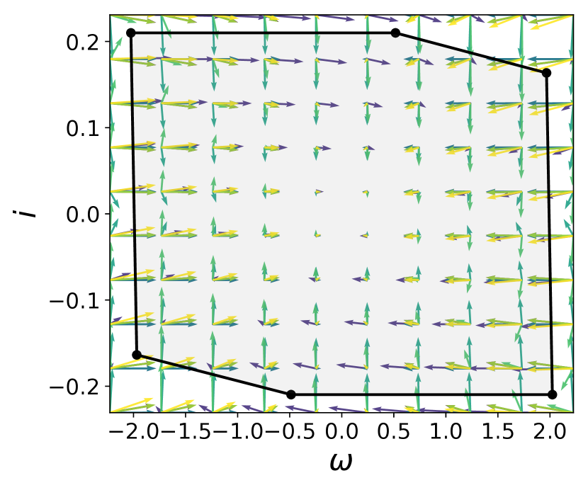
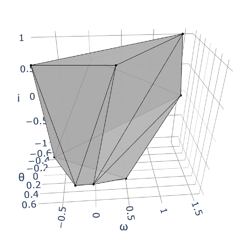
Figure 1: Left: Invariant polyhedron for (25) and (26),
for $\gamma_{s}=10$ ($\eta\geq 0.07$). Right: Invariant polyhedron for (27) and (29), with $\gamma_{p}=4$ and $u$ as in (30) ($\eta\geq 0.004$, $0.03$ for nominal)

We next consider the DC motor position example. The dynamics are now:

$$\frac{d}{dt}\begin{bmatrix}\theta\\ \omega\\ i\end{bmatrix}=\begin{bmatrix}0&1&0\\ 0&-b/J&K/J\\ 0&-K/L&-R/L\end{bmatrix}\begin{bmatrix}\theta\\ \omega\\ i\end{bmatrix}+\begin{bmatrix}0\\ 0\\ 1/L\end{bmatrix}u$$ (27)

And we assume that we can only measure $\theta$ and $i$:

$$y=\begin{bmatrix}1&0&0\\ 0&0&1\end{bmatrix}\begin{bmatrix}\theta\\ \omega\\ i\end{bmatrix}$$ (28)

We also have parameter perturbations of the form

$$J\in[J_{0}/\gamma_{p},\gamma_{p}J_{0}],\,K\in[K_{0}/\gamma_{p},\gamma_{p}K_{0}],$$ (29)

with $\gamma_{p}=4$.

Using our algorithm we find that we simultaneously stabilise these under a common Lyapunov function using output feedback law

$$u=\begin{bmatrix}-19.7&-18.7\end{bmatrix}y$$ (30)

The identified polyhedron is also shown in Fig. 1 and has only 9 vertices.

VIII Conclusions and Future Work

We presented an algorithm for finding polyhedral Lyapunov functions of fixed complexity for feedback design.

We believe that this can be used to tackle interesting research directions. We plan to extend the theory to open systems and interconnections, and apply it to the nonlinear contraction setting.

References

- [1] University of Michigan control Tutorials for MATLAB and Simulink. https://ctms.engin.umich.edu/CTMS/index.php?aux=Home.
- [2] R. Ambrosino, M. Ariola, and F. Amato. A Convex Condition for Robust Stability Analysis via Polyhedral Lyapunov Functions. 50(1):490–506.
- [3] F. Blanchini and S. Miani. Set-Theoretic Methods in Control. Systems & Control: Foundations & Applications. Birkhäuser, 2 edition.
- [4] S. Boyd, L. El Ghaoui, E. Feron, and V. Balakrishnan. Linear Matrix Inequalities in System and Control Theory. Studies in Applied and Numerical Mathematics. Society for Industrial and Applied Mathematics.
- [5] S. Boyd and L. Vandenberghe. Convex Optimization. Cambridge University Press.
- [6] F. Clarke. Lyapunov Functions and Feedback in Nonlinear Control. In M. S. Queiroz, M. Malisoff, and P. Wolenski, editors, Optimal Control, Stabilization and Nonsmooth Analysis, volume 301 of Lecture Notes in Control and Information Sciences, pages 267–282. Springer Berlin Heidelberg.
- [7] G. B. Dantzig. Origins of the simplex method. In S. G. Nash, editor, A History of Scientific Computing, pages 141–151. ACM.
- [8] A. L. Dontchev and R. T. Rockafellar. Implicit Functions and Solution Mappings: A View from Variational Analysis. Springer Monographs in Mathematics. Springer New York.
- [9] F. Forni and R. Sepulchre. A Differential Lyapunov Framework for Contraction Analysis. 59(3):614–628.
- [10] N. Guglielmi, L. Laglia, and V. Protasov. Polytope Lyapunov Functions for Stable and for Stabilizable LSS. 17(2):567–623.
- [11] D. Kousoulidis and F. Forni. An Optimization Approach to Verifying and Synthesizing K-cooperative Systems. In 21st IFAC World Congress (IFAC-V 2020).
- [12] W. Lohmiller and J. Slotine. On Contraction Analysis for Non-linear Systems. 34(6):683–696.
- [13] P. McMullen. The maximum numbers of faces of a convex polytope. 17(2):179–184.
- [14] S. Miani and C. Savorgnan. MAXIS-G: A software package for computing polyhedral invariant sets for constrained LPV systems. In Proceedings of the 44th IEEE Conference on Decision and Control, pages 7609–7614.
- [15] J. Nocedal and S. J. Wright. Numerical Optimization. Springer Series in Operations Research. Springer, 2nd ed edition.
- [16] A. Pavlov, N. van de Wouw, and H. Nijmeijer. Uniform Output Regulation of Nonlinear Systems: A Convergent Dynamics Approach. Systems & Control: Foundations & Applications. Birkhäuser, 2005.
- [17] A. Polański. On absolute stability analysis by polyhedral Lyapunov functions. 36(4):573–578.
- [18] G. Russo, M. Di Bernardo, and E. Sontag. Global entrainment of transcriptional systems to periodic inputs. PLoS Computational Biology, 6(4):e1000739, 04 2010.